Article

An Integrated Dynamical Modeling Perspective for Infrastructure Resilience

1
IRSTEA, UR LISC, 9 Avenue Blaise Pascal, 63170 Aubiere, France
2
RENEW Institute, 108 Cooke Hall, University at Buffalo, Buffalo, NY 14260-1660, USA
3
Qatar Transportation and Traffic Safety Center, College of Engineering, Qatar University, Doha, Qatar
4
School of Sustainable Engineering, Arizona State University, Tempe, AZ 85281, USA
*
Author to whom correspondence should be addressed.
Infrastructures 2018, 3(2), 11; https://doi.org/10.3390/infrastructures3020011
Submission received: 1 March 2018 / Revised: 30 April 2018 / Accepted: 3 May 2018 / Published: 9 May 2018
(This article belongs to the Special Issue Resilient Infrastructure Systems)

Abstract

:
This paper considers a dynamical way to connect resilience outcomes and processes by nesting process-based approaches inside a controlled dynamical system under resource constraints. To illustrate this, we use a dynamical model of electric power generation to show the complementary aspects of outcome, resources, and process-based approaches for analyzing infrastructure resilience. The results of this stylized model show that adaptation is the most influential process and that for monitoring to be efficient it must account for associated costs. Beyond these specific results, we suggest that nesting outcome- and process-based approaches within a dynamical controlled framework can be very useful and complementary for infrastructure managers and designers tasked with effectively allocating resources for enhancing system resilience.

1. Introduction

The impact of extreme weather events (such as floods or cyclones) is of growing concern for managing infrastructure systems, due to the growing economic losses associated with a growing population and a changing climate [1,2]. For instance, the damage caused by US hurricanes has increased considerably during the second half of the 20th century, reaching a cost of about one hundred billion dollars per year [3]. This trend is expected to be accelerated by the increase in the frequency and intensity of extreme events during the 21st century [4]. This increase of global losses and the pessimistic scenarios of future climate change have led decision-makers to evolve in terms of risk analysis: they have progressively transitioned from reliability analysis to resilience.
The main difference between reliability and resilience approaches is that reliability focuses on avoiding failure, such as safety protocols for nuclear power plants [5], where failure can yield catastrophic damage. In contrast, resilience also considers the recovery of the infrastructure system function after an extreme event. For instance, the National Academy of Sciences definition of resilience is based on the cycle of “plan, absorb, recover and adapt” [6]. The National Infrastructure Advisory Council gives a similar multi-part definition of resilience [7] based on robustness, resourcefulness, recovery, and adaptation. However, the interpretation of the concepts of resilience still remains ambiguous (and sometimes conflicting). Thus, there is a need for operational tools that can help decision-makers clarify these concepts for analyzing infrastructure resilience. The challenge for providing such tools is that among existing studies on resilience, there is continuous tension regarding how resilience is analyzed and assessed. The ability to analyze resilience critically depends on the underlying conceptual framework (based on outcomes or processes, for instance) used for the analysis.
Outcome-based approaches are mainly used for measuring the effectiveness of policies in a quantitative way and for measuring the resilience of infrastructure exposed to floods [8] or water systems [9], for instance. The use of outcomes facilitates resilience communication to a wide audience and can be easily tracked over time in order to assess changes within the system and to evaluate policy [10]. On the other hand, process-based approaches [11] aim to qualitatively improve the resilience processes involved, such as adaptation capacity or institutional learning. Moreover, process-based approaches often emphasize the role of people and the management of institutions responsible for the physical infrastructure. For example, adaptation and learning are processes that are likely to be employed by those that plan for and maintain infrastructure, and not by the physical infrastructure itself [11].
Despite its importance, the assessment of resilience processes may be more difficult in practice than outcome-based assessments. While the latter may require as little as a basic sensor to track system state variables, processes can only be observed in action or via in-depth case studies after an event occurs. In practice, both approaches are complementary for improving the resilience analysis of the system. Process-based approaches require outcomes for evaluating their effectiveness, and improving resilience outcomes undoubtedly depends on system processes. However, formal frameworks, which bridge both approaches, have seldom been proposed. To the knowledge of the authors, only static approaches that associate an outcome to a given process have been developed, such as the “resilience matrix approach” [12]. Only one recent study [13] attempts to propose quantitative measures that represent processes using dynamical networks. The purpose of this work is to go further, by not only having quantitative measures but also by proposing a controlled dynamical framework for explicitly highlighting the connections between technical outcomes and processes in a dynamical way. We argue that one of the main drawbacks of current approaches, which connect outcomes and processes, is that the dynamical side of infrastructure is not explicitly taken into account. We argue that such a framework that combines outcome- and process-based methodologies in a dynamical way will offer new insights for infrastructure resilience analysis.
Here, we present a methodology that nests a process-based approach within a dynamical controlled system framework [14]. The main contribution of this work is to have an integrated view of resilience that considers outcome- and process-based approaches under resources constraints (see Figure 1). To illustrate our view, we use the “Sensing-Adapting-Anticipating-Learning” (SAAL) framework for assessing resilience processes [11] for illustrating our view. However, other process-based frameworks may be used without changing the overall methodology proposed here. In addition, we consider the critical role that resource constraints (e.g., financial resources) may play in constraining infrastructure resilience options. This framework is applied on a stylized power system to identify the strengths and the weaknesses of the combined approach. The purpose of this stylized model is not to fully address the resilience management of power infrastructure but to show how to apply our perspective approach to an infrastructure system. It enables us to illustrate how outcomes and processes are dynamically related through the lens of resilience. We then perform a sensitivity analysis on the system to identify the most influential processes for improving resilience outcomes in a quantitative way. Beyond the specific results from the stylized power system example, we argue that our perspective methodology is valuable for assessing resilience for other types of infrastructure systems.

2. Bridging Outcomes and Processes Concepts in a Dynamical Way

2.1. The Outcome-Based Approach Using a Dynamical Controlled System Framework

While resilience remains a useful concept, defining suitable metrics may be confusing (even conflicting) due to the diversity of situations from which resilience concepts are used. Also, many resilience metrics or outcomes are static, i.e., they do not depend on time. However, infrastructure systems are dynamical systems that evolve in time according to their own properties, as well as changing environmental conditions (i.e., aging, wearing, climate change, and demand). In other words, infrastructure systems have to adopt self-organizing structures, which are the strongest form of resilience [15]. In this regard, management strategies should enable decision-makers to keep desirable properties of the infrastructure system and create a self-organizing infrastructure system. Several mathematical frameworks, i.e., dynamical controlled system frameworks, were developed in order to define or evaluate these management strategies according to different criteria. Among these different mathematical frameworks, the dynamical controlled system framework based on viability theory [14] has been successfully used for analyzing environmental management issues such as managing fisheries [16], exploited forests [17], or social networks [18], as well as mitigating lake eutrophication [19] or climate change [20]. Dynamical controlled approaches have also been effective for analyzing social-technical systems such as hydrological systems [21] or urban transportation systems [22]. In both cases, systems may evolve in time in different ways, and it is necessary to define the time range of interest; long-term objectives may yield different strategies than those defined from short-term objectives. This time of interest, denoted T, remains a subjective issue that depends on the studied infrastructure. If the present time is t 0 , we are interested in what happens between t 0 and t 0 + T (we consider that t 0 = 0 for simplicity and clarity). A dynamical control system is based on causal loop approaches from which a control is added. Causal loops enable us to highlight interactions and causality in system dynamics in order to identify unexpected systemic behavior [23]. In our approach, we consider a closed-loop system, i.e., the controls depend on the current state of the infrastructure.
For modeling the dynamics of the infrastructure according to time, we suggest that the system can be described by a vector x ( t ) of state variables at time t . A state variable is defined as a variable used to describe the mathematical “state” of a dynamical system. This state variable describes the system to determine its future state and can be assessed by dynamical equations, mainly differential equations. Note that the value of the state variable x(t + 1) often only depends on the state x(t) (called Markovian process). This vector x(t) also represents the properties of interest that describe the system. For instance, if we consider a system that generates electric power, the state variables may represent the amount of electricity supplied per day, which reflects the service quality of the power system.
In addition to system state variables, it is necessary to model the technological characteristics of a network, represented here as the vector p(t), which, for example, could correspond to the capacity of the transmission lines required to distribute the generated electricity. Unlike the state variable, the parameter vector p(t) does not require a differential equation for predicting its future states, because either the parameters are constant or their evolutions are imposed (forcing equation). Also, we must consider a decision vector u ( t ) representing the independent variables that represent actions taken by decision-makers. This decision vector u ( t ) enables decision-makers to influence the dynamics of the state variable x(t). For example, in the case of electric power system, decisions can be related to building new infrastructure to meet increasing demand. We define a set of admissible decisions U ( t ) such as u ( t ) U ( t ) , t . In other words, only a set of limited decisions are possible in our simplified model. In addition, we consider here adaptive management (in what follows, adaptive management and adaptation process may be confusing. Therefore, here adaptive management is used for designating a management according to the states of the system, whereas adaptation process is one of the four processes of the SAAL approach [11]) [24,25], i.e., the control u(t) may change at each time step according to the state of the system, but it also requires different social processes, such as learning, in order to be efficient [25].
Drivers that stress the system are represented as the vector w ( t ) . These can be difficult to identify in practice because of a lack of measurement, unexpected processes, or internal noise. These drivers can be either exogenous or internal to the system. Internal drivers may be variations in electricity production due to component failures or regular maintenance, as well as exogenous drivers from extreme weather and/or climate change - increased temperatures, for example, can impact the peak energy demand [26], as well as reduce the efficiency of power plants and electricity transmission).
We choose here to adopt a discrete dynamical framework:
x ( t + 1 ) = f ( x ( t ) , u ( t ) , w ( t ) , p ( t ) )
The function f determines how the infrastructure evolves according to the time t . It represents how the infrastructure runs, and this function describes interactions between its current state x ( t ) , the decision variables u ( t ) , and the unexpected drivers w ( t ) that may yield the failure of the infrastructure. For the sake of clarity, we only consider exogenous drivers in what follows. These drivers may be slow, such as climate change, or fast, such as hurricanes or flooding. Fast exogenous drivers are mainly unexpected, whereas it is easier to adapt the infrastructure system to slow drivers. The main issue is the trade-off between the dynamics of the threats, the dynamics of the infrastructure, and the dynamics of the human processes. To mitigate the effects of the drivers w ( t ) on the system, the purpose is therefore to define all policies either for keeping the functions of the infrastructure (reliability-oriented policy) or for recovering these functions if they are lost (resilience-oriented policy). However, it is necessary to clearly define the functions and the properties of interest we want to preserve (or to recover) through a criterion c ( t ) . This criterion constitutes the objectives of the decision-makers. This objective can be a function to optimize or a constraint to comply with. For instance, in the case of power systems, a simple criteria can be the number of outages or the cumulated time of outages within a given time period. Then, the objective can be the minimization of outages (optimization) or having a maximum number of outages per year (constraints). Both approaches are valuable, depending on the infrastructure and the resources allocated. Defining such criteria is based not only on economic issues but also on values and beliefs of the decision-makers, for instance, what is the maximum number of outages that is acceptable relative to the population? Then, the policy cycle aims at developing policy for keeping (or recovering) this criterion c ( t ) , which is a measurement of the difference of “how is” the system (i.e., the current state of the system) and “how should be” the system (i.e., the desirable system state).
We use this framework as the skeleton of the dynamics of the system and for classifying the outcomes of our system in a simple way:
-
State variables x(t): the properties of interest in our system (e.g., energy produced) that represent the dynamics of the infrastructure.
-
Decision variables u(t): variables that we can change and that influence the dynamics of our infrastructure (e.g., building a new power infrastructure).
-
Criteria c(t): the management objectives (e.g., having a low number of outages). It also evaluates the difference between the current and desirable states of the system.
-
Exogenous drivers w(t): the events that may affect the infrastructure (e.g., slow changes such as climate change or fast changes such as flooding).
-
System parameters p(t): the main characteristics of the system (e.g., energy production per day).
-
Dynamics of the system f: interactions between previous outcomes (e.g., interaction between a new infrastructure, outages, and climate change).
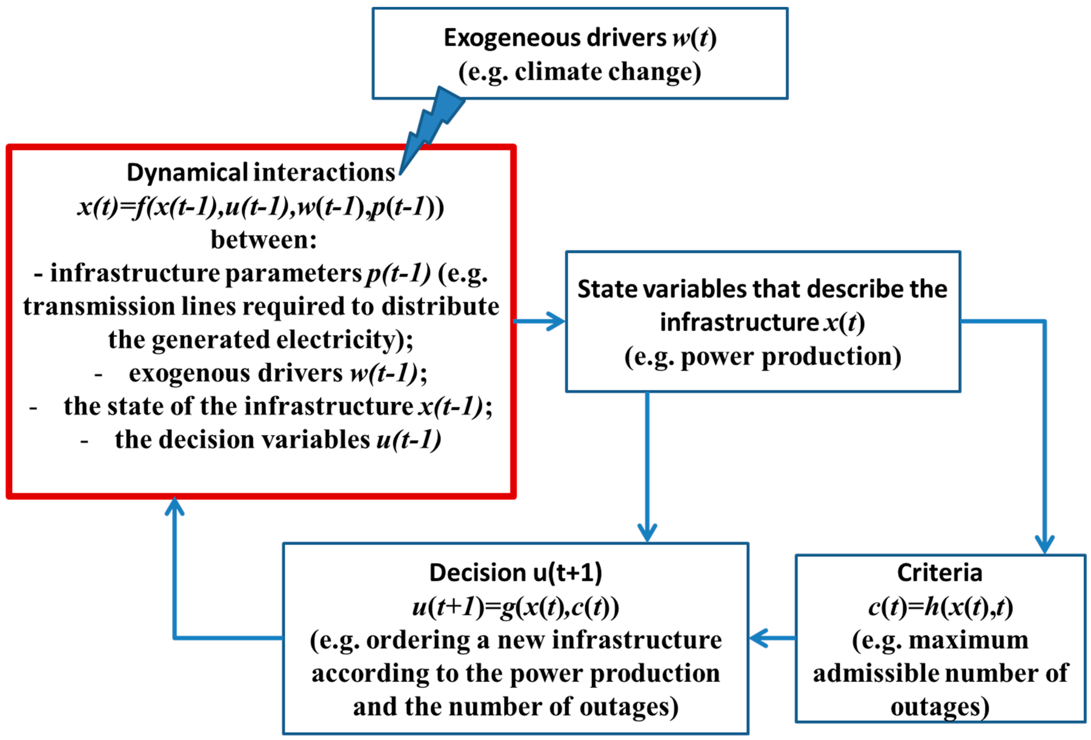
With the key outcomes defined for our framework, the next step is to integrate processes into the outcome-based approach in Figure 2.

2.2. Process-Based Analysis of Infrastructure Resilience

The notion of resilience as a process began within the discipline of ecology and has since been applied to non-ecological systems. One of the most cited perspectives from ecology comes from Holling [9], who contends that ecosystems are highly dynamic and that resilience arises in the ability of these systems to absorb internal and external shocks and maintain relationships in the face of change. In other words, it is the instability of a system’s behavior, combined with its capacity to maintain critical relationships despite that instability, which determines its resilience. This is distinct from the traditional perspective that equates ecological resilience with stability. In this view, resilience is the ability of a system to return to equilibrium after a disturbance and can be analyzed based on the fluctuation around an equilibrium state. Although this approach lends itself to quantitative analytics, Holling argues that it is insufficient for considering the realistic behavior of complex ecological systems characterized by non-linearity, heterogeneity, and random events. Alternatively, he argues that a more meaningful approach to resilience would recognize our inability to precisely and quantitatively predict the future and would instead focus on developing systems that can qualitatively accommodate unexpected future events [9]. Applying these ecological observations to socio-technical systems suggests a management-based approach to resilience that requires organizing, planning, and coordinating systems in ways that allow them to be adaptive and flexible.
Thinking about resilience as a process is reflected in recent work on topics of modeling and policy related to socio-ecological systems [27], improving organizational management [28,29,30,31], and informing risk and disaster management efforts [32,33]. The process of managing knowledge systems—i.e., production, validation, circulation, and consumption—and its importance for decision-making that promotes resilience has also been acknowledged [34]. Moreover, a conceptual framework offered by Hollnagel et al. [35] outlines a process whereby a system’s resilience is reflected by its ability to (1) know what to look for (monitor); (2) know what to expect (anticipate); (3) know what to do (respond); and (4) know what happened (learn), during key points of design, operation, and management of technical systems.
A management perspective complicates the study of resilience. Just as Holling described the complexity of ecological systems, socio-technical systems are complex adaptive systems that are characterized by emergent behaviors and uncertain futures, including feedback loops, non-linear interactions, path dependencies, and stochastic influences [14]. In addition, strategic interactions, individual and spatial heterogeneity, and varying timescales pose challenges to modeling these complex systems [27]. This complexity makes risk analysis, the traditional approach to understanding system vulnerabilities, insufficient for understanding system resilience. Risk analysis necessitates the ability to evaluate the probability of future events (in a quantitative or qualitative way), which is dependent on using the frequency and intensity of past events [36], as well as personal judgement on what might change to predict future trends. Alternatively, the resilience of socio-technical systems requires preparing for unexpected, unknown, and unidentifiable hazards, and underscores the notion that the past is an insufficient predictor of future vulnerability [14]. This view of resilience involves continuous, iterative, and adaptive management, as well as comfort with ambiguity and incomplete understanding.
Additionally, managing resilience implies adopting a safe-to-fail approach for unexpected hazards. Safe-to-fail strategies emphasize adaptability rather than robustness using a variety of strategies for infrastructure design, such as multi-functionality, redundancy, and modularization; diversity of social and biological systems; multi-scale networks and connectivity; and adaptive planning and design [37]. Following Hollnagel et al. [35] and Park et al. [14], we propose that managing resilient, safe-to-fail socio-technical systems requires four recursive processes: sensing, anticipating, adapting, and learning. We define these processes below:
  • Sensing is the process by which new system stresses are efficiently and rapidly incorporated into current understanding. Sensing allows decision-makers to determine the proper state of essential systems variables.
  • Anticipation is the process by which newly incorporated knowledge gained by sensing is used to foresee possible crises and disasters. Anticipation allows decision-makers to imagine multiple future states to which the system may evolve or transition. Anticipation explores possibility, rather than probability [38]. Then, as more information becomes available, potentiality yields to prediction, anticipation yields to forecast, and resilience analysis may yield to risk.
  • Adaptation is the response taken after information from sensing and anticipation is incorporated into understanding. Adapting is a process of changing either the design variables or constraint conditions under which a system operates to achieve a higher value performance state.
  • Learning is the process by which new knowledge is created and maintained by observation of past actions, that is, understanding how various adaptive strategies have succeeded to buffer, delay, or attenuate the variability arising from both internal and external factors. After adaptation, the level of appropriateness of adaptive actions can be assessed, and future iterations can incorporate this knowledge.
It is these four recursive processes that articulate the authors’ approach to thinking about resilience as a management process for understanding and improving the resilience of socio-technical systems. In this perspective paper, we use the “SAAL” approach, but other process-based frameworks can be used without changing the main insights of this paper, i.e., connecting outcomes and processes in a dynamical way.

2.3. Allocating Resources

Resilience resources can be generally understood as material buffers, system redundancies, or internal capabilities [12,39,40]. For energy distribution systems, important resources include back-up generation or emergency fuel storage. Here we focus on the resources involved with infrastructure management that could constrain system resilience, including economic resources (e.g., money needed for building a new infrastructure), manpower (e.g., capacity for repairing damages after an extreme event), and time (e.g., the time required for building a new infrastructure). These resources are obviously interdependent (e.g., more money may yield more manpower and therefore less maintenance time) and constrained (e.g., yearly overall budget to comply with). However, resources are not necessarily quantitative and/or static. It is important to pool resources at the right time and at the right locations to prevent system failures during an event. Resource allocation remains a complex problem depending on the infrastructure considered and how that system evolves over time [41]. Decision-makers continually grapple with resources allocation for improving resilience. By including resource constraints in our framework, our formal approach may be useful for better understanding effective resource allocation among system processes and outcomes.

2.4. Nesting Processes Inside a Controlled Dynamical System

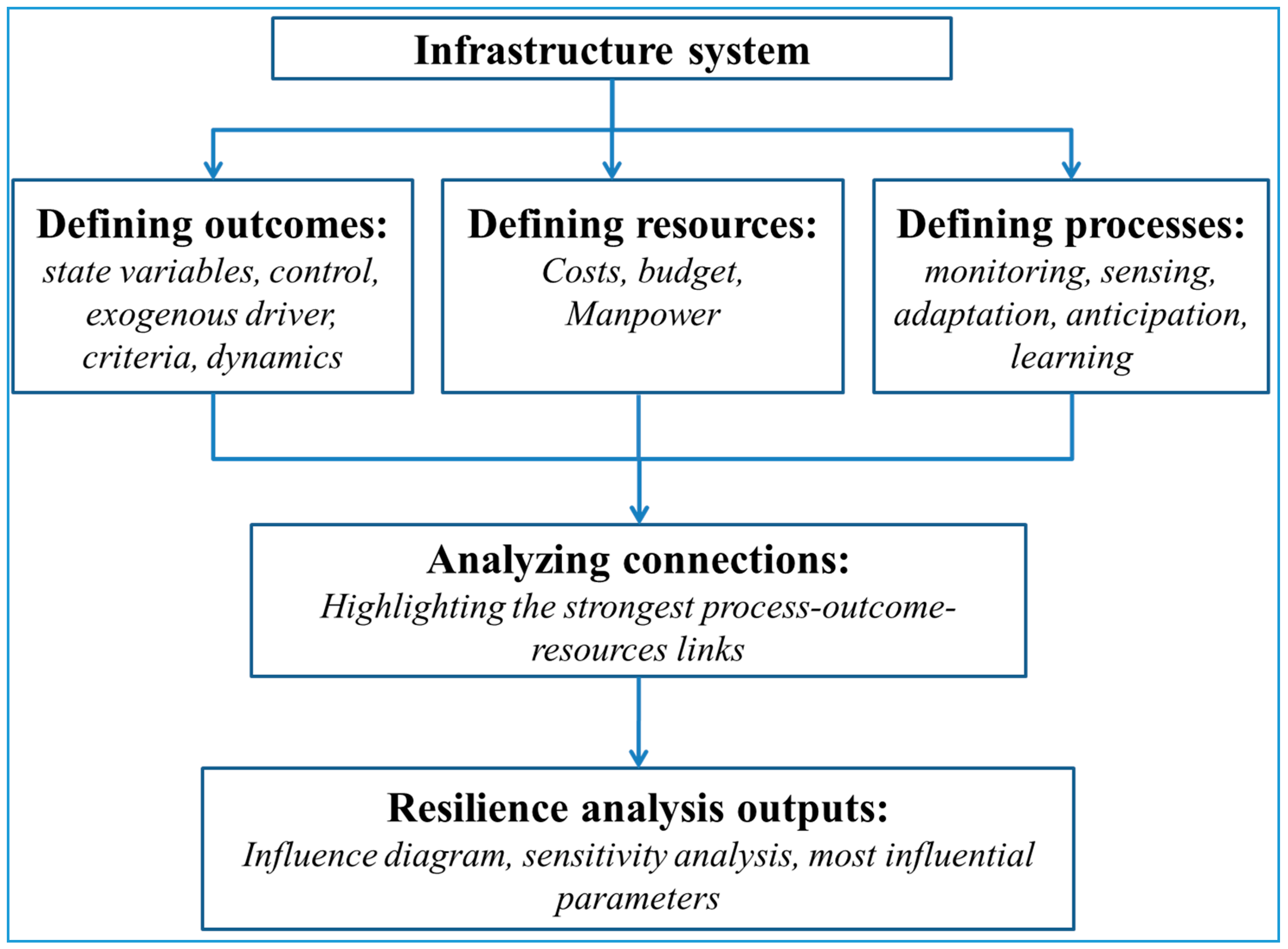
As explained above, the purpose of this perspective framework is to highlight connections between outcomes, processes, and resources in a dynamical way. We propose four steps to defining the system under study, which are illustrated by Figure 3:
-
(i) Describe the system in terms of outcomes: What is the criteria? What are the decision and state variables of the infrastructure systems?
-
(ii) Describe the system in terms of processes: Which part of system mainly contributes to sensing, adaptation, anticipation, and learning?
-
(iii) Describe the system in terms of resources: How much and where are the resources allocated in the infrastructure?
-
(iv) From (i), (ii), and (iii), qualitatively analyze the connections between the identified outcomes and processes under resource allocations through analysis. Only the strongest links are considered;
-
(v) From (iv), highlight these connections through an influence diagram.
Once this analysis is complete, a sensitivity analysis from a resilience point of view is performed to inform the resilience of the system by highlighting the most influential processes and associated costs.
To illustrate our approach, we apply it to a stylized model of electric power generation in the next section to analyze its resilience. The purpose is to clearly define the context, the objectives, and the dynamics of this system, as well as the main processes. The model aims to test processes (sensing, monitoring, adaptation, anticipation, and learning) associated with long-term resilience management of power infrastructure system to extreme events and increasing peak energy demand as a result of climate change.

3. A Stylized Model of Electric Power Generation

The system contains a power infrastructure system and the institution managing the power infrastructure, such as the energy utility company. The main goal of the model is to meet the electricity demand under various cases including disturbance due to extreme events. In our case, we focus on slower climate change impacts to infrastructure, but the approach may be applied in cases of faster, extreme weather events and disturbances as well. The simulation timeframe is from 2000 to 2060. The institution needs to utilize several tools based on processes and outcomes to manage the infrastructure and the resilience of the entire system using these mechanisms.
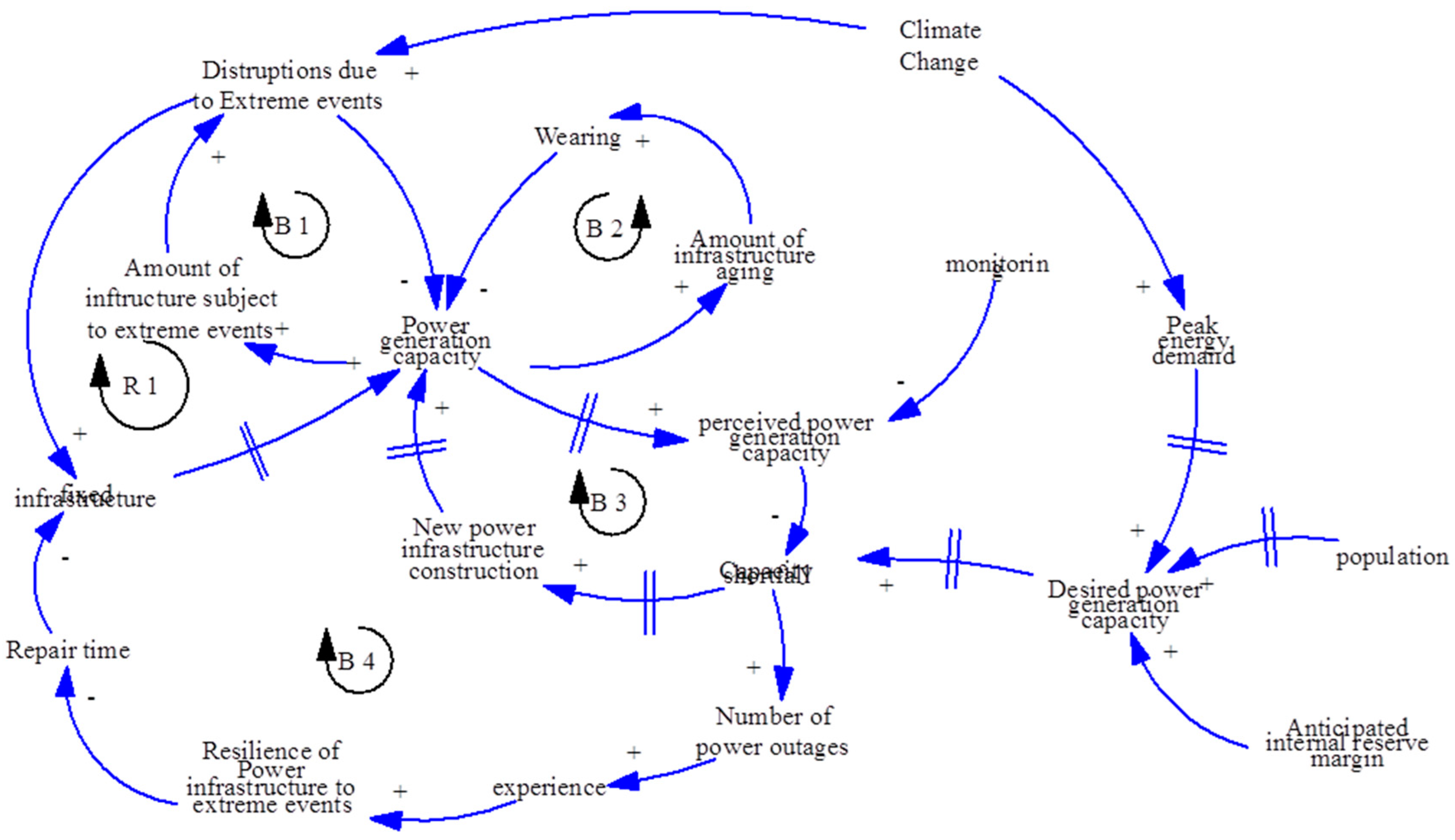
The model (Figure 4) is a simplified compact model showing the capacity of power generation system to meet the required demand under the pressure of disturbances due to climate change. The state variable is the capacity, i.e., nameplate capacity in MW. The disturbance will occur based on climate change pressures, which can be efficiency losses due to increased ambient temperature, increased likelihood of wildfires, permanent loss of production due to damage of critical infrastructure, etc. The institution needs to monitor the system and then decide the system improvement needed (e.g., additional generation capacity) based on the discrepancy between perceived power generation capacity and perceived demand. The key concept here is the information delays within the system. The goal is to control these delay times and find the optimal time control management strategy. There are three types of delays within the system: (1) perception delay, (2) response delay, and (3) physical delay.
Perception delay is a function of monitoring frequency. As the user observes the system more frequently, their ability to sense and perceive the losses will increase. Second, when managers know what the capacity increase will be, they may not place that order right away. The response delay reflects the partial adjustments over time. The third is the physical delay during the power infrastructure improvement, which can be time to construct a new power plant, as well as to fix a certain damaged component of the power generation system. In addition, there is another perception delay related to forecasting the future peak demand. This delay reflects the information delay in between data collection, processing, and forecasting. The main mechanism regulating this system is explained in the following sub-section.
There are five mechanisms (loops) regulating this system. Most of the variables in these loops are under the effect of exogenous drivers such as increasing population, rising temperature, and extreme events due to climate change. Figure 4 shows the causal loop diagram of the hypothetical system, in which the relationships among the key variables are presented.
The model has four balancing loops and one reinforcing loop:
Loop B1: Power generation capacity → (+) amount of infrastructure subject to extreme events → (+) disruptions due to extreme evens → (−) power generation capacity. If the power generation capacity is increased, the amount of infrastructure (power plants, transmission lines, etc.) subject to extreme events increases. If there is higher exposure to extreme events, there are higher disruptions in power generation and transmission. In this loop, the number of extreme events observed is a function of rising temperatures resulting from climate change, which is an exogenous driver in this loop.
Loop B2: Power generation capacity → (+) amount of infrastructure aging → (+) wearing → () power generation capacity. Similarly, if power generation capacity increases, there would be more infrastructure aging and total wearing of physical infrastructure. The wearing is a physical degradation of infrastructure, and it decreases the power generation capacity.
Loop B3: Power generation capacity → (+) perceived adequacy power generation capacity → (−) perceived capacity shortfall → (+) new power infrastructure construction → (+) power generation capacity. This balancing loop represents the adaptation cycle of the system, in which there are delays due to perception and monitoring frequency of the actual infrastructure. Nevertheless, if the power generation capacity increases, the perceived power generation capacity would increase sooner or later, depending on how frequently we observe the degradation in the system. If the perceived generation capacity increases, the capacity shortfall decreases, or vice versa. Capacity shortfall is also a function of desired power generation capacity due to increasing population and increasing peak energy demand due to warmer temperatures. Population is also an exogenous driver in this model. If the capacity shortfall increases, there will be a need for new infrastructure, and eventually the system will try to adapt to new conditions and meet the new demand. In this loop, delays and anticipation of extreme events play very important roles. Considering that there will be inevitable delays such as construction delay, response delays, and perception delays about the existing state of the system, increasing the internal reserve margin as a buffer plays crucial role.
Loop B4: Power Generation Capacity → (+) perceived power generation capacity → (−) capacity shortfall → (+) number of power outages → (+) experience → (+) resilience of power infrastructure to extreme events → (−) repair time → (−) fixed infrastructure → (+) power generation capacity. This loop follows the same path as the capacity shortfall with the balancing loop 3. If the capacity shortfall increases, the number of power outages increases. In the model, we introduced a variable called experience, which increases as the system managers observe a power outage due to extreme event and capacity shortfall. The variable experience is a function of learning behavior (See Figure 4). These variables will be explained in more detail in the following sub-section. As experience increases, the resilience of power infrastructure due to extreme events will be greater. The resilience of the power infrastructure is expressed in two main mechanisms. First, the time required to fix infrastructure is decreased as a function of experience. Second, damage to power infrastructure will be less after it is exposed to an extreme event. As the repair time decreases, the fixed infrastructure per unit of time increases, and therefore power generation capacity increases.
Loop R1: Power generation capacity → (+) amount of infrastructure subject to extreme events → (+) disruptions due to extreme evens → (+) fixed infrastructure → (+) power generation capacity. If the power generation capacity increases, the amount of infrastructure subjected to extreme events will be greater, which increases the probability of disruptions due to extreme events. If the disruptions due to extreme events increase, the rate of fixing infrastructure increases, and so the power generation capacity increases. There is a trade-off between the number of disruptions and the rate of fixing infrastructures.
The main model consists of one stock and seven delayed flows regulating the stock of power generation capacity. There is also a sub-model to calculate peak energy demand, which is a function of population and peak temperature (see Appendix A). Critical model parameters and their brief descriptions are presented in Table 1.

4. Analysis of the Power Infrastructure Resilience

4.1. Reference Scenario

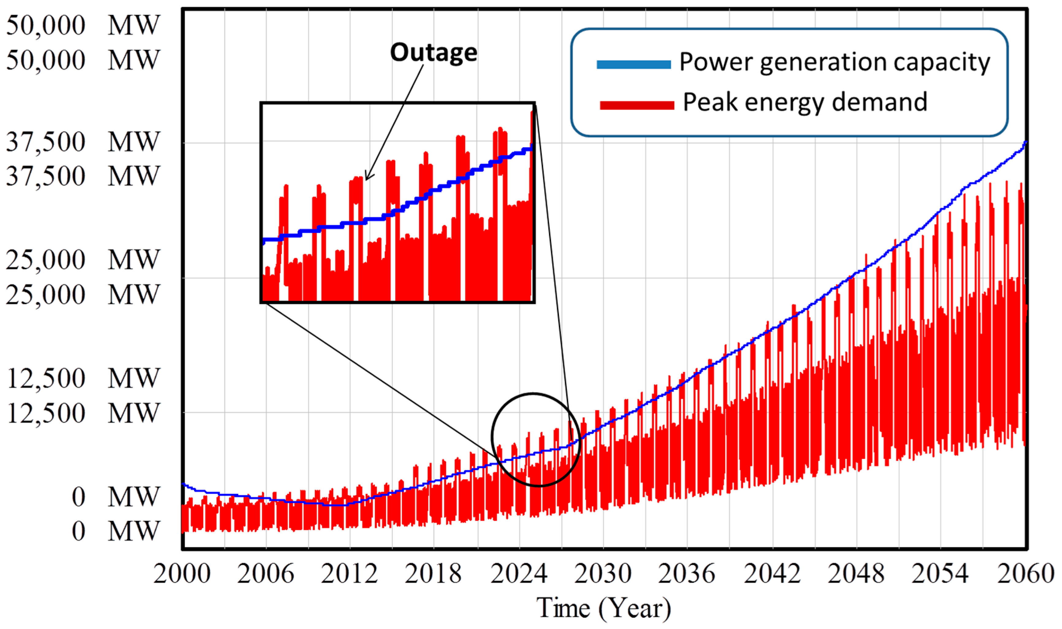
We model the dynamics of the system with the initial parameters (see Table 1). Figure 5 shows the dynamics of the peak energy demand and the power generation capacity.
Results show that the power generation capacity does not always meet the peak energy demand, especially during the summer where the peak energy demand is highest. Many outages occur during our time of interest (2000 to 2060) but note that the number of outages decreases after 2050 (power generation is higher than peak energy demand). The fluctuations in electricity demand are mainly due to seasonal differences. In summer months, the peak electricity demand is significantly higher than that of in winter months. The number of outages decreases towards 2060 for several reasons. First, the system learns overtime. Second, the trend in population slightly changes (as well as demand) after 2050. The decrease in the population growth allows the infrastructure system to be less stressed (trade-off between the capacity of building new infrastructure and the population growth) after 2050 yielding less outage. Note that importing electricity is not taken into consideration in this study.

4.2. Dynamical Analysis of the System’s Outcomes and Processes

We aim at defining a strategy to: (1) limit the number of outages; and (2) come back into a desirable state of the system when there is an outage. Table 2 describes the processes examined as routes towards reducing outages.
From this table, we analyze the connections using the following process flow:
  • When the infrastructure is first monitored: monitoring depends on both technological issues (acquisition time) and subjective values (mainly based on experience). The state variables x ( t ) give a representation of the state of the infrastructure based here on the wearing of the infrastructure;
  • Once the infrastructure has been monitored, the outcomes are sensed in a different way according to experience and sensitivity. It corresponds to the transformation of x ( t ) to s ( x ( t ) ) , the s function being the “sensing function”. If there is no sensing, s is the identity function. In our stylized model, we consider that the wearing may be sensed in different ways by the managers;
  • We consider the anticipation process as the wish to intervene in the system according to sensing in order to change the dynamics of the system through the desired margin;
  • Decision-makers may take into account the state of the system and adapt the current policies to this state, but also to criteria c ( t ) . The control u ( t ) is applied on the system, i.e., a new power infrastructure order;
  • The system is monitored to better understand its endogenous mechanisms and how the system can be controlled. This is the learning process that enables improvement in the efficiency of repair.
It is important to note that this flow is not sequential. Process and outcome assessment are done in a simultaneous way, and all functions are not completely mathematically defined. For instance, the social parameters that represent beliefs and values are difficult to quantify.
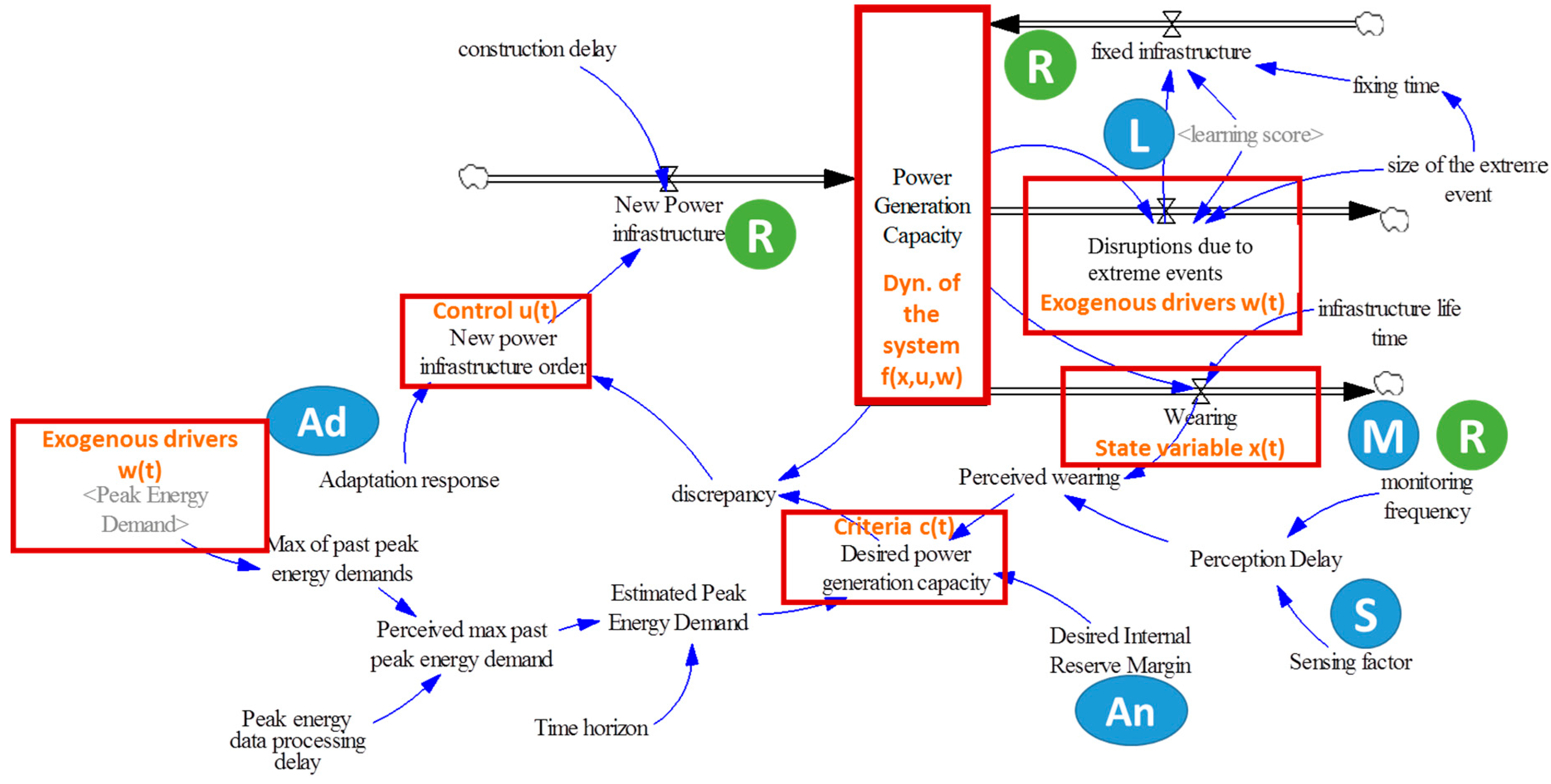
Figure 6 represents the influence diagram of the power infrastructure with the SAAL processes incorporated within the dynamical controlled system framework in the case of our stylized power system. We recall that the locations of the processes (listed in Table 2) clearly depend on the studied system, and they can dramatically change from one system to another according to the considered problem.

4.3. Sensitivity Analysis of the Processes

Sensitivity analysis is traditionally used to highlight the most influential parameters in models. There are mainly two types of analysis. The first one, called “local analysis”, describes the function of the model around some initial variable values. However, such analysis does not explore the whole input space. In the 1980s, to overcome the limitations local analysis, “global analysis” techniques were developed [42] based on the variation of the input parameters over the entire space of uncertainty. Among global analysis, Sobol indices [42] were used in environmental sciences [43]. We perform a global sensitivity analysis (based on Sobol indices, see Appendix B for more details) on the parameters that modeled our processes according to the total duration of outages (outcome). For this purpose, we change the reference values (see Table 1) by ±20%. Sobol indices are represented in Figure 7a.
Results show that adaptation is the most influential process, followed by the anticipation process: both processes represent 97% of the sensitivity of the system in terms of outages. This is due to the fact that even low monitoring and low learning are sufficient for making decisions because of the relative slow dynamics of the exogenous drivers (climate change and population growth). Indeed, our toy model only considers slow changes for the sake of clarity, but we can expect that fast changes (such as hurricanes) may enable monitoring process to be more influential. Thus, we can release efforts on the other processes (monitoring and learning) in order to reinforce adaptation and anticipation. Moreover, the second-order Sobol indices (representative of potential coupling between processes) are very low. Processes are quasi-independent in our case and there is no synergy between processes in order to improve the resilience of the system. Results indicate that increasing adaptation may decrease the total duration of outages by 2.5 times (see Figure 7b), whereas monitoring barely affects the system (Figure 7c).
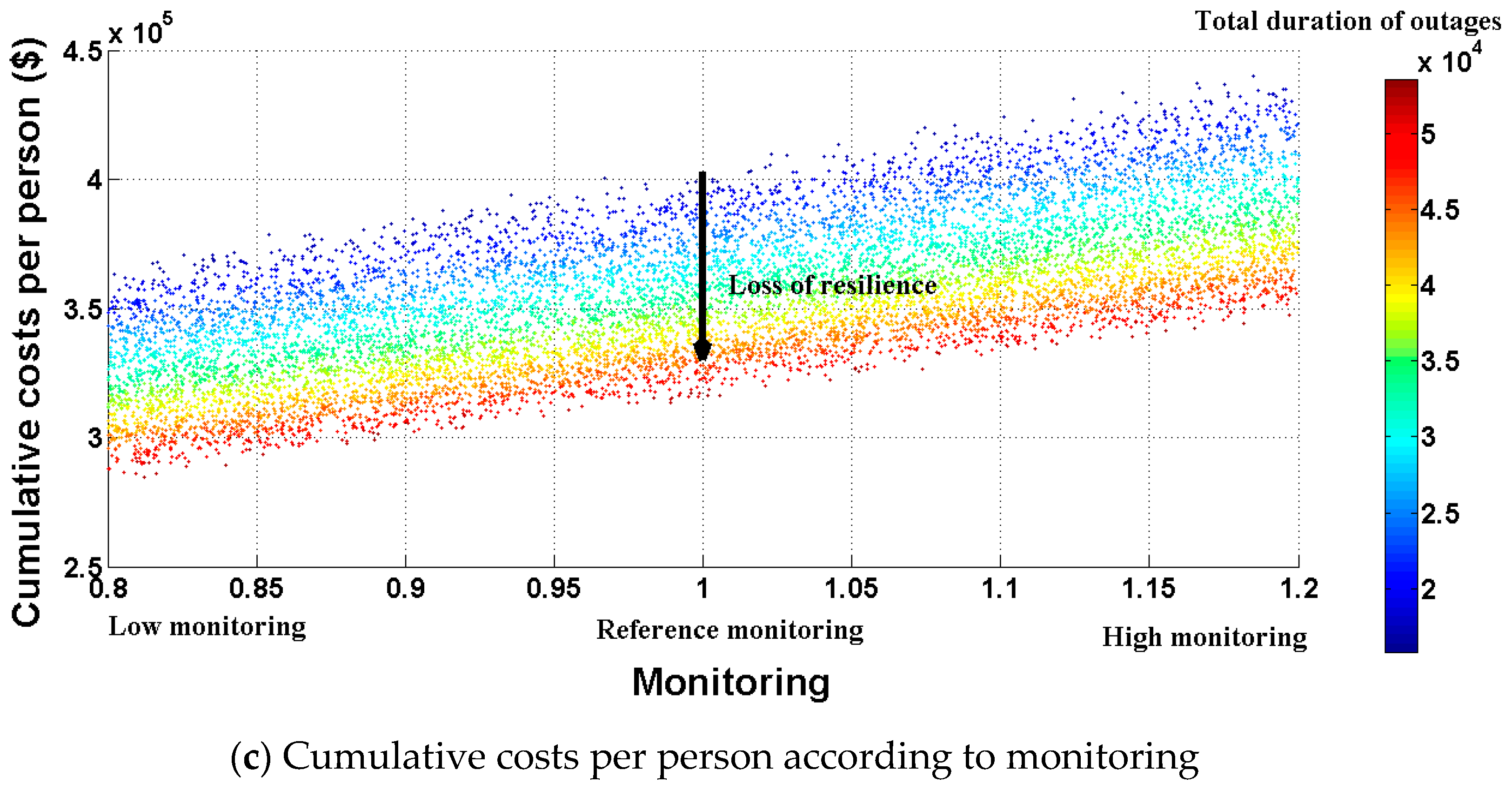
Our sensitivity analysis on the resources (i.e., costs) involved in infrastructure management (see Figure 8) shows that monitoring and adaptation greatly affect the costs, following by the anticipation process. These results are due to the costs associated with the different processes and naturally depend on the specifics of the monitoring process employed (monitoring done by human or by sensor, etc.). Here, it is the monitoring process that is the most influential process (in terms of resources), although this process does not influence the total duration of outages (see Figure 8c). This analysis emphasizes the need to move efforts from monitoring to adaptation in order to improve resilience and decrease the costs (see Figure 8b,c). However, it should be noted that the analyzed system is a generic power generation system relying on a set of assumptions presented in Appendix B. Hence, findings can vary depending on the analyzed system and the associated costs.

5. Discussion and Conclusions

The analysis of infrastructure resilience remains an ongoing challenge for alleviating the increasing global losses caused by climate change and extreme weather. Our perspective view aims to assist managers in their decision processes, as well as to help engineers to better design more resilient infrastructure systems. It is based on the state of the infrastructure yielding an adaptive management approach for achieving infrastructure resilience. In other words, our framework does not require complete knowledge about the perturbation to the system, because the decisions are made post-perturbation for system adaptability. Therefore, adaptive management, as we propose here, constitutes the system capacity to manage infrastructure subjected to extreme weather events (or other kinds of events), for which it is difficult to forecast the probability of occurrence. Applying our dynamical approach to a stylized power system shows that resources should be allocated toward adaptation response over monitoring because of the nature of the changes considered here. This result illustrates how our perspective framework can be helpful for decision makers to identify important interactions between outcome and processes of specific systems and how to effectively allocate limited resource to improve infrastructure resilience.
We think that our dynamical framework is applicable to other infrastructure systems that are vulnerable to uncertain impacts of climate change, such as water distribution systems. Depending on the system of interest, the model parameters require adjustment. For example, to model a water system, the main goal would be altered to reflect the service of interest, such as water demand, water quality, or water pressure of the system. The criteria c(t) can also be a nonlinear function of these three indicators, according to the real problem in order to be representative of the service quality. The causal loops would also have to be adjusted to reflect the relationships between the new system parameters and system behavior. The nature of exogenous drivers w(t) and internal factors of the system would likely remain the same or similar, as climate change and extreme weather, as well as population growth, are common stressors to most physical systems. Internal factors related to aging infrastructure and wearing are also relevant in most other contexts. Moreover, the control mechanisms of the system by the institution would remain unchanged, with monitoring times, order of system improvements, and perceived system states as important tools. Although adjustments are necessary, we are confident that the notion of integrating outcome-based with process-based resilience perspectives is worthwhile for a range of physical infrastructure systems, especially for thinking about alternatives for investment beyond physical infrastructure remedies.
Although simplistic, our perspective provides a first attempt at reconciling outcome and process-based analysis of resilience by merging a dynamical controlled framework with a process-based approach. One drawback of our current framework is that it is too simplistic; the infrastructure systems we seek to model are inherently complex and increasingly interdependent with other systems. Other systemic approaches may be used for improving the insights provided by our approach: infrastructure resilience can be seen from (a) a system-of-systems perspective [44] and (b) a perspective of the different phases of infrastructure development [45]. For example, electrical power systems are physically integrated with water systems, since water is necessary to generate electricity, and electricity is required to pump and distribute water. Also, our communication networks and cyber systems link both the water and energy system digitally. This means that a disruption or failure in either system can cause disruptions or failures in the other [46]. Thus, future work is needed to integrate more complexity, including more complex non-linear feedbacks, GIS modeling, more complex exogenous drivers such as water availability, other energy sources, other infrastructure components, etc. Allowing for simulating interdependency between systems may potentially yield unexpected consequential failures of several infrastructure systems. Institutional dynamics and structures may also yield failures as much as physical factors. In Hurricane Katrina, for example, institutional failures and social patterns in housing exacerbated the physical infrastructure failures and slowed overall recovery [47]. It is therefore necessary to go further in the analysis of institutional resilience- by using an adaptive management approach to address the issues of infrastructure resilience. Applying our perspective framework to real case studies would be a natural next step for testing and validating the model.
Nevertheless, this approach requires interdisciplinary research and collaboration at the intersection of mathematics (such as control theory and caul loop modeling), engineering (physical infrastructure system knowledge), and social sciences (such as assessing belief and values of decision-makers for defining normative issues), yielding inherent difficulties in terms of communication or objective issues. However, methods for improving infrastructure resilience of critical systems are a research space ripe for interdisciplinary work. Infrastructure systems are inherently socio-technical; they are characterized by physical infrastructure (i.e., components like pipes and transducers), but designed, managed, maintained, and planned for by organizations and institutions (i.e., utilities, regulations, private, and public influences). By integrating the quantitative, outcome-based approach with the process, qualitative-based methods, we argue that our dynamical approach is an initial step towards implementing a cross-disciplinary and systems-analysis based heuristic for the purpose of increasing both the social and technical aspects of infrastructure resilience.

Author Contributions

All authors have contributed equally to the paper.

Acknowledgments

This work was supported by a grant from NSF RIPS (NSF Award Search: Award#1441352), a grant from the National Research Institute of Science and Technology for Environment and Agriculture (France), and a grant from the French National Research Agency (project VIRGO, ANR-16-CE03-0003-01 grant).

Conflicts of Interest

The authors declare no conflict of interest.

Appendix A. Model Information

Initial model values and mathematical formulations (Vensim built in functions) are presented as follows:
  • Adaptation response = 6
    • Units: Year
  • Construction delay = 10
    • Units: years
  • Desired Internal Reserve Margin = 0.15
    • Units: %
  • Desired power generation capacity = (perceived peak energy demand + perceived wearing) × (1 + desired internal reserve margin)
    • Units: MW
  • Discrepancy = Desired power generation capacity-power generation capacity
    • Units: MW
  • Distributions due to extreme events = power generation capacity × size of the extreme event× (1/learning score)
    • Units: MW/Year
  • Experience = IF THEN ELSE (learning behavior < 1, learning behavior, 1) × total number of outages experienced due to extreme events
    • Units: dmnl
  • Fixed infrastructure = DELAY1 (distributions due to extreme events, fixing time/learning score)
    • Units: MW/Year
  • Fixing time = WITH LOOKUP (size of the extreme event,
    • ([(0, 0)–(0.25, 5)], (0, 0), (0.0165138, 0.4), (0.0330275, 0.6), (0.0559633, 0.8),
    • (0.0793578, 1.1), (0.104128, 1.3), (0.12844, 1.38158), (0.15367, 1.71053),
    • (0.179664, 2.30263), (0.220183, 3.46491), (0.25, 5)))
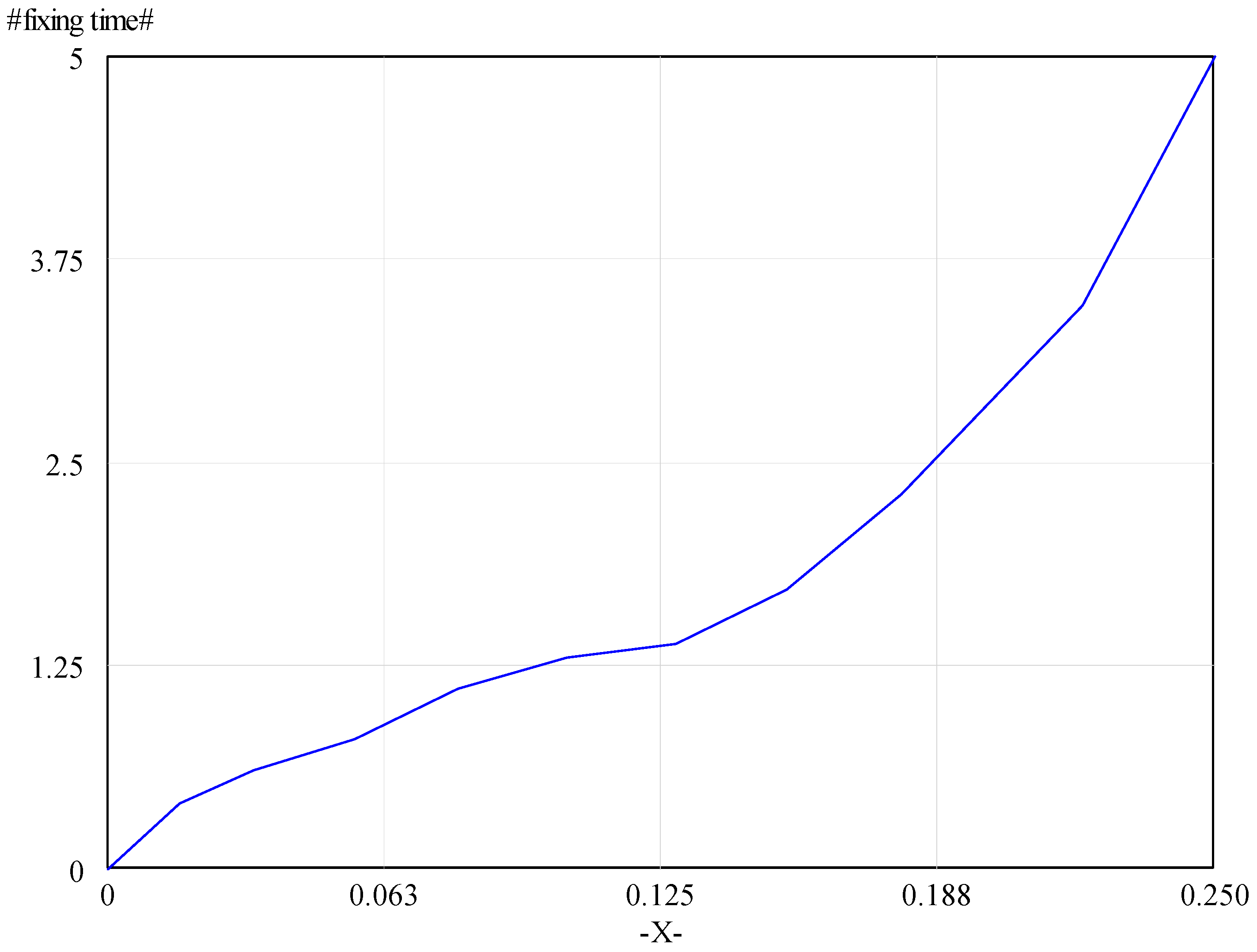
Figure A1 shows the relationship in between fixing time (y axis) and the size of the extreme event (x axis).
Figure A1. Relationship between fixing time and size of extreme event.
Infrastructures 03 00011 g0a1
Size of extreme event is a percentage of the power infrastructure affected. So, the maximum value of this variable is 25%, indicating that an extreme event can affect maximum 25% of the existing power infrastructure.
  • Infrastructure life time = 25
    • Units: Year
  • Estimated peak energy demand = FORECAST (perceived max past peak energy demand, 10, time horizon)
    • Units: MW
  • Time horizon = 10
    • Units: Year
  • Max of past peak energy demands = SAMPLE IF TRUE (max of past peak energy demands < peak energy demand, peak energy demand, peak energy demand)
    • Units: MW
  • Peak energy data processing delay = 1
    • Units: year
  • Peak energy demand = Per capita energy demand × population
    • Units: MW
  • Perceived max past peak energy demand = DELAY FIXED(max of past peak energy demands, peak energy data processing delay, max of past peak energy demands)
    • Units: MW
  • Learning behavior = 0.5
    • Units: learning rate per event
    • Learning rate, [0, 1] no learning = 0; moderate learning = 0.5; high Learning = 1
  • Learning score = WITH LOOKUP (experience,
    • ([(0, 0)–(60, 3)], (0, 1), (1.83486, 1.23684), (4.0367, 1.53947), (6, 1.76316),
    • (10, 2.03947), (14.8624, 2.27632), (20, 2.44737), (25, 2.57895), (30, 2.68421), (35, 2.77632),
    • (40, 2.84211), (45, 2.88158), (48.6239, 2.89474), (51.3761, 2.90789), (54.6789, 2.92105), (60, 3)))
    • Units: dmnl
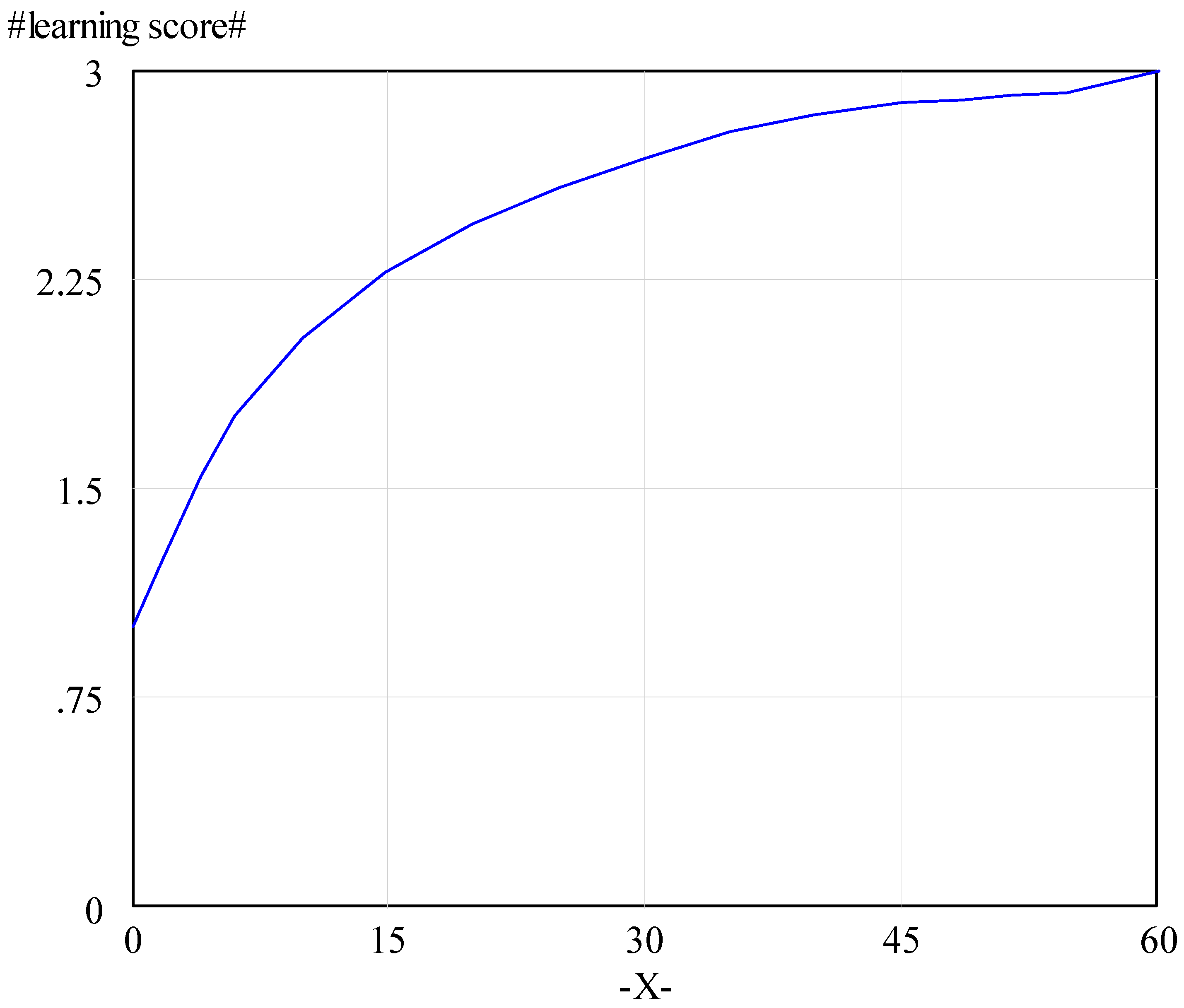
Learning score varies between 1 and 3, indicating improvement in fixing take up to 1/3 and strength of infrastructure to disruptions due to extreme events up to 3 times. The minimum learning score of 1 indicates that there is no improvement in both fixing time and strength of infrastructure.
Figure A2 shows the relationship in between learning score (y axis) and experience (x axis).
Figure A2. The relationship between learning score (y axis) and experience (x axis).
Infrastructures 03 00011 g0a2
  • Monitoring frequency = 6
    • Units: times in a year
  • New power infrastructure = DELAY FIXED (new power infrastructure order, construction delay, 0)
    • Units: MW/Year
  • New power infrastructure order = MAX (discrepancy/adaptation response, 0)
    • Units: MW
  • Perceived wearing = SMOOTH (wearing, perception delay)
    • Units: MW
  • Perception Delay = WITH LOOKUP (monitoring frequency,
    • ([(0, 0)–(12, 100)], (0, 100), (1, 30), (2, 20), (3, 10), (3.97554, 7.01754), (5, 5.26316), (6, 3.94737), (8, 2.63158), (9, 1.75439), (12, 1)))
    • Units: Year
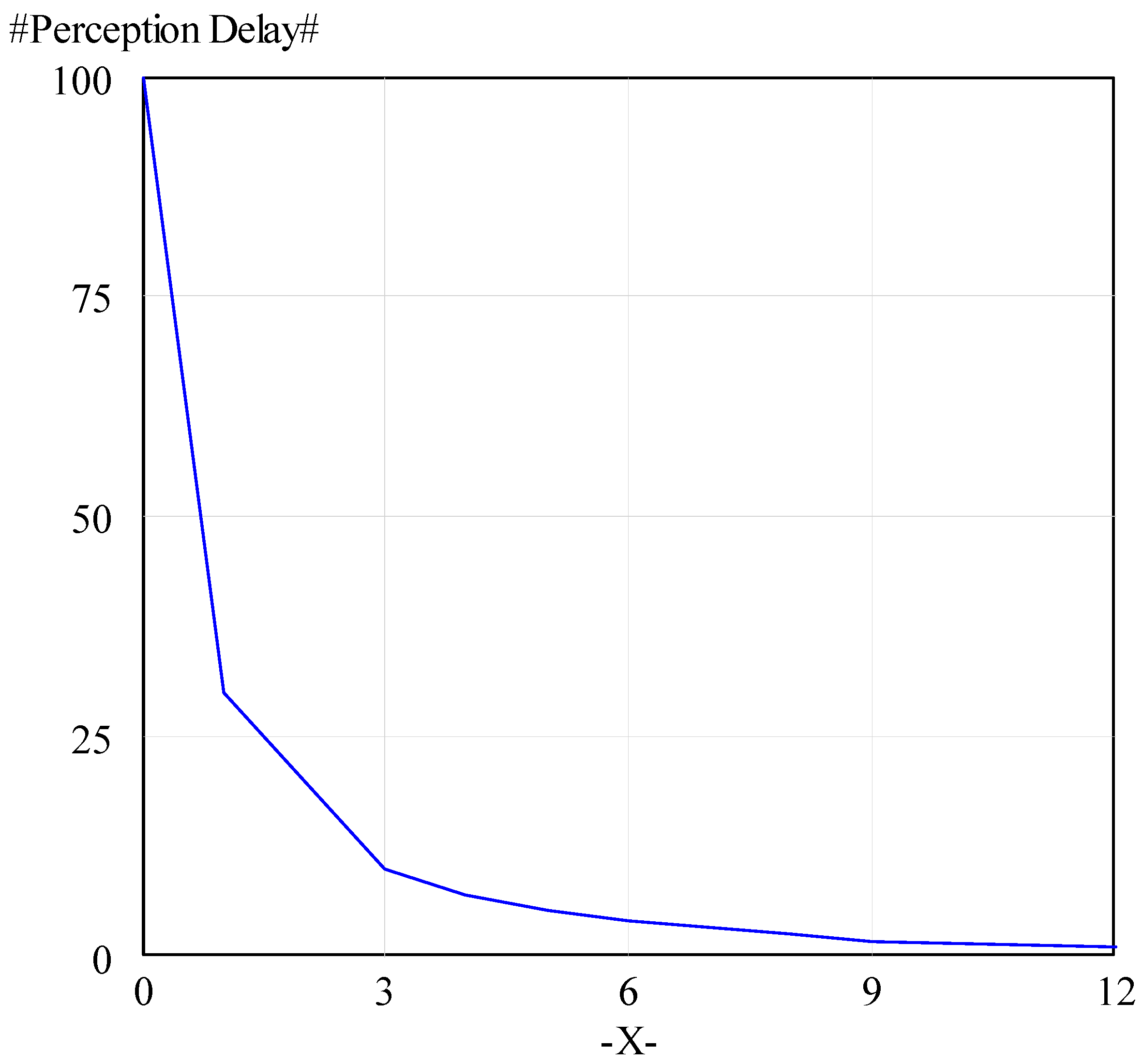
The relationship between monitoring frequency and perception delay is shown in Figure A3.
Figure A3. The relationship between perception delay (y axis) and monitoring frequency (x axis).
Infrastructures 03 00011 g0a3
  • Power generation capacity = INTEG (new power infrastructure + fixed infrastructure-distributions due to extreme events-wearing, 3000)
    • Units: MW
  • Size of the extreme event = A FUNCTION OF (size of the extreme event)
    • Size of the extreme event = RANDOM NORMAL (0.001, 0.25, 0.02, 0.05, 0.01)
    • Units: {%}
    • Percentage of the power generation capacity under extreme impact
  • TIME STEP = 0.0625 (the time step for the simulation
    • Units: Year
  • Total number of outages experienced due to extreme events = INTEG (number of outages experienced due to extreme events, 0)
    • Units: times
  • Wearing = power generation capacity/infrastructure life time
    • Units: MW/Year
  • Effect of temperature change on per capita energy demand = WITH LOOKUP (peak temperature/normal peak temperature,
    • ([(0, 0)–(1, 1)], (0, 0), (0.12844, 0.0394737), (0.266055, 0.0657895), (0.342508, 0.109649), (0.40367, 0.153509), (0.489297, 0.210526), (0.504587, 0.223684), (0.605505, 0.328947), (0.672783, 0.425439), (0.746177, 0.539474), (0.788991, 0.635965), (0.859327, 0.767544), (0.923547, 0.864035), (0.993884, 0.986842)))
    • Units: fraction
Effect of temperature change on per capita peak energy demand is shown in normalized values in Figure A4. Normalization is made by dividing the corresponding years’ values by the maximum values.
  • Normal peak temperature = 45
    • Units: C
    • Maximum peak temperature
  • Normal per capita energy demand = 0.006
    • Units: MW/person
    • Per capita energy demand at 45 degrees Celsius max temperature
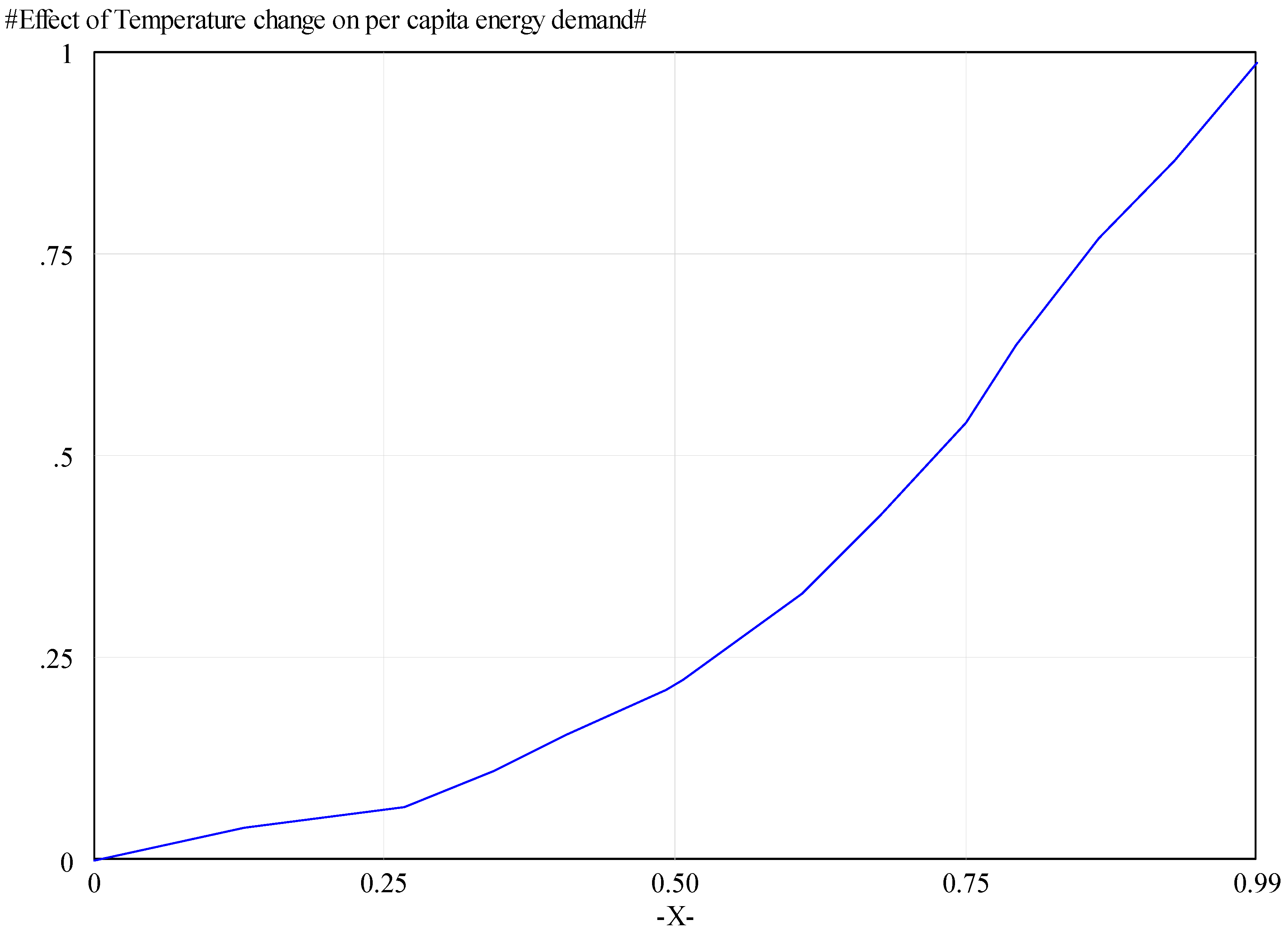
Figure A4. Normalized effect of temperature change on per capita energy demand.
Infrastructures 03 00011 g0a4
  • Peak temperature = ACTIVE INITIAL (IF THEN ELSE (Time >= 2016, temperature after 2016, temperature before 2016), 37.21)
    • Units: Celsius
  • Summer time = PULSE TRAIN (first pulse time, duration , repeat interval , last pulse time)
    • Units: dmnl
    • Pulse train function is used to model summer and winter times.
  • Repeat interval = 1
    • Units: Month
  • First pulse time = 2000.5
    • Units: Month
  • Last pulse time = 2060
    • Units: Month
  • Growth fraction = ([(2000, 0) (2060, 0.06)], (2000, 0.01), (2005, 0.015), (2010, 0.02), (2014.86, 0.0313158), (2020, 0.04), (2030.09, 0.0428947), (2044.95, 0.0344737), (2059.82, 0.0192105))
    • Units: %
  • Growth rate = Population*growth fraction (time)
    • Units: person
  • Per capita Energy Demand = ACTIVE INITIAL (IF THEN ELSE (summer time = 1, normal per capita energy demand × effect of temperature change on per capita energy demand × summer time, winter peak energy demand), 0.003)
    • Units: MW/person
  • Population = INTEG (growth rate, 1 × 10⁶)
    • Units: person
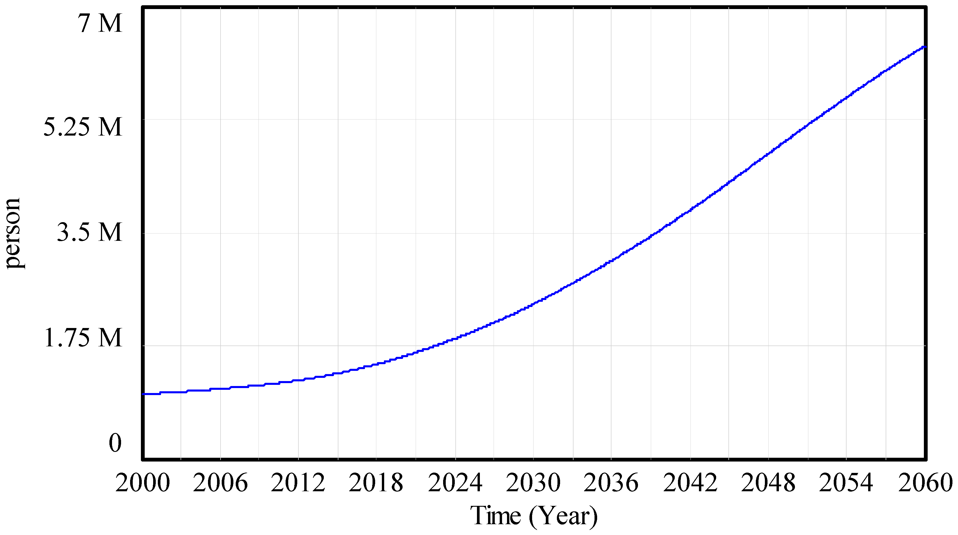
Figure A5 shows the population growth for this hypothetical model.
Figure A5. Population change over time.
Infrastructures 03 00011 g0a5
  • Temperature after 2016 = RANDOM NORMAL (35, 45, 40.6, 1, 37)
    • Units: Celsius
  • Temperature before 2016 = RANDOM NORMAL (33, 43, 37.21, 0.87, 37)
    • Units: Celsius
  • Winter peak energy demand = RANDOM NORMAL (0.0015, 0.004, 0.003, 0.005, 0.001)
    • Units: MW

Appendix B. Sobol Indices

Sensitivity analysis is here used in order to highlight the most influential parameters in stylized power system model. We used a “global analysis” technique based on the variation of the input parameters over the entire space of uncertainty, called “Sobol indices” (42). We perform a global sensitivity analysis (based on Sobol indices) on our processes Xi according to outcome Yj (here the costs and the total duration of outages). First-order Sobol indices of parameter are:
SI i j = V ar ( E ( Y j | X i ) V ar ( Yj )
For evaluating the Sobol indices, we use a linear meta-model Y j ^ (X) of Yj:
Y j ^ ( X ) = α 0 j + k = 1 12 α k j X k
This linear model well matches the numerical data (R > 0.99), yielding the direct calculation of the Sobol indices as follows:
SI i j = ( α i j ) 2 k = 1 12 ( α k j ) 2

References

  1. Bouwer, L.M. Have disaster losses increased due to anthropogenic climate change? Bull. Am. Meteorol. Soc. 2011, 92, 39–46. [Google Scholar] [CrossRef]
  2. Easterling, D.R.; Meehl, G.A.; Parmesan, C.; Changnon, S.A.; Karl, T.R.; Mearns, L.O. Climate extremes: Observations, modeling, and impacts. Science 2000, 289, 2068–2074. [Google Scholar] [CrossRef] [PubMed]
  3. Pielke, R., Jr.; Gratz, J.; Landsea, C.; Collins, D.; Saunders, M.; Musulin, R. Normalized Hurricane Damage in the United States: 1900–2005. Nat. Hazards Rev. 2008, 9, 29–42. [Google Scholar] [CrossRef]
  4. Nicholls, R.J. Coastal flooding and wetland loss in the 21st century: Changes under the SRES climate and socio-economic scenarios. Glob. Environ. Chang. 2004, 14, 69–86. [Google Scholar] [CrossRef]
  5. Martorell, S.; Sanchez, A.; Serradell, V. Age-dependent reliability model considering effects of maintenance and working conditions. Reliab. Eng. Syst. Saf. 1999, 64, 19–231. [Google Scholar] [CrossRef]
  6. National Academy of Science. Disaster Resilience: A National Imperative; The National Academies Press: Washington, DC, USA, 2012. [Google Scholar]
  7. National Infrastructure Advisory Council. Critical Infrastructure Resilience—Final Report and Recommendations; National Infrastructure Advisory Council: Washington, DC, USA, 2009.
  8. Kotzee, I.; Reyers, B. Piloting a social-ecological index for measuring flood resilience: A composite index approach. Ecol. Indic. 2016, 60, 45–53. [Google Scholar] [CrossRef]
  9. Hashimoto, T.; Stedinger, J.R.; Loucks, D.P. Reliability, resiliency, and vulnerability criteria for water resource system performance evaluation. Water Resour. Res. 1982, 18, 14–20. [Google Scholar] [CrossRef]
  10. Seager, T.P.; Satterstrom, F.K.; Linkov, I.; Tuler, S.P.; Kay, R. Typological Review of Environmental Performance Metrics (with Illustrative Examples for Oil Spill Response). Integr. Environ. Assess. Manag. 2007, 3, 310–321. [Google Scholar] [CrossRef] [PubMed]
  11. Park, J.; Seager, T.P.; Rao, P.S.C.; Convertino, M.; Linkov, I. Integrating Risk and Resilience Approaches to Catastrophe Management in Engineering Systems. Risk Anal. 2013, 33, 356–367. [Google Scholar] [CrossRef] [PubMed]
  12. Linkov, I.; Eisenberg, D.; Bates, M.; Chang, D.; Convertino, M.; Allen, J.; Flynn, S.; Seager, T. Measurable resilience for actionable policy. Environ. Sci. Technol. 2013, 47, 10108–10110. [Google Scholar] [CrossRef] [PubMed]
  13. Ganin, A.A.; Massaro, E.; Gutfraind, A.; Steen, N.; Keisler, J.M.; Kott, A.; Mangoubi, R.; Linkov, I. Operational Resilience: Concepts, Design and Analysis. Sci. Rep. 2016, 6, 19540. [Google Scholar] [CrossRef] [PubMed]
  14. Aubin, J.P. Viability Theory; Birkhauser Boston Inc.: Cambridge, MA, USA, 1991. [Google Scholar]
  15. Meadows, D.H.; Wright, D. Thinking in Systems: A Primer; Chelsea Green Publishing: White River Junction, VT, USA, 2008. [Google Scholar]
  16. Brias, A.; Mathias, J.-D.; Deffuant, G. Accelerating viability kernel computation with CUDA architecture: Application to bycatch fishery management. Comput. Manag. Sci. 2016, 13, 371–391. [Google Scholar] [CrossRef]
  17. Mathias, J.D.; Bonté, B.; Cordonnier, T.; DeMorogues, F. Using the viability theory for assessing flexibility of forest managers under ecological intensification. Environ. Manag. 2015, 56, 1170–1183. [Google Scholar] [CrossRef] [PubMed]
  18. Mathias, J.D.; Lade, S.J.; Galaz, V. Multi-level policies and adaptive social networks—A conceptual modeling study for maintaining a polycentric governance. Int. J. Commons 2017, 11, 220–247. [Google Scholar] [CrossRef]
  19. Rougé, C.; Mathias, J.D.; Deffuant, G. Extending the viability theory framework of resilience to uncertain dynamics, and application to lake eutrophication. Ecol. Ind. 2013, 29, 420–433. [Google Scholar] [CrossRef]
  20. Mathias, J.D.; Anderies, J.M.; Janssen, M. On our rapidly shrinking capacity to comply with the planetary boundaries on climate change. Nat. Sci. Rep. 2017, 7, 42061. [Google Scholar] [CrossRef] [PubMed]
  21. Khan, S.; Yufeng, L.; Ahmad, A. Analysing complex behaviour of hydrological systems through a system dynamics approach. Environ. Model. Softw. 2009, 24, 1363–1372. [Google Scholar] [CrossRef]
  22. Wang, J.F.; Lu, H.P.; Peng, H. System dynamics model of urban transportation system and its application. Jiaotong Yunshu Xitong Gongcheng Yu Xinxi. J. Trans. Syst. Eng. Inform.Technol. 2008, 8, 83–89. [Google Scholar]
  23. Montgomery, M.; Broyd, T.; Cornell, S.; Pearce, O.; Pocock, D.; Young, K. An innovative approach for improving infrastructure resilience. Proc. Inst. Civil. Eng. Civil. Eng. 2012, 165, 27–32. [Google Scholar] [CrossRef]
  24. Folke, C.; Hahn, T.; Olsson, P.; Norberg, J. Adaptive governance of social-ecological systems. Ann. Rev. Environ. Resour. 2005, 30, 441–473. [Google Scholar] [CrossRef]
  25. Pahl-Wostl, C. Transitions towards adaptive management of water facing climate and global change. Water Resour. Manag. 2007, 21, 49–62. [Google Scholar] [CrossRef]
  26. Bartos, M.D.; Chester, M.V. Impacts of climate change on electric power supply in the Western United States. Nat. Clim. Chang. 2015, 5, 748–752. [Google Scholar] [CrossRef]
  27. Anderies, J.M.; Folke, C.; Walker, B.; Ostrom, E. Aligning key concepts for global change policy: Robustness, resilience, and sustainability. Ecol. Soc. 2013, 18, 8. [Google Scholar] [CrossRef]
  28. Weick, K.E.; Sutcliffe, K.M. Managing the Unexpected: Resilient Performance in an Age of Uncertainty; John Wiley & Sons: Hoboken, NJ, USA, 2011; Volume 8. [Google Scholar]
  29. Bhamra, R.; Dani, S.; Burnard, K. Resilience: The concept, a literature review and future directions. Int. J. Prod. Res. 2011, 49, 5375–5393. [Google Scholar] [CrossRef]
  30. Linnenluecke, M.; Griffiths, A.; Winn, M. Extreme Weather Events and the Critical Importance of Anticipatory Adaptation and Organizational Resilience in Responding to Impacts. Bus. Strategy Environ. 2011, 21, 17–32. [Google Scholar] [CrossRef]
  31. Madni, A.M.; Jackson, S. Towards a conceptual framework for resilience engineering. Syst. J. IEEE 2009, 3, 181–191. [Google Scholar] [CrossRef]
  32. Chang, S.E.; McDaniels, T.; Fox, J.; Dhariwal, R.; Longstaff, H. Toward Disaster-Resilient Cities: Characterizing Resilience of Infrastructure Systems with Expert Judgments. Risk Anal. 2014, 34, 416–434. [Google Scholar] [CrossRef] [PubMed]
  33. Norris, F.H.; Stevens, S.P.; Pfefferbaum, B.; Wyche, K.F.; Pfefferbaum, R.L. Community resilience as a metaphor, theory, set of capacities, and strategy for disaster readiness. Am. J. Commun. Psychol. 2008, 41, 127–150. [Google Scholar] [CrossRef] [PubMed]
  34. Miller, C.A.; Munoz-Erickson, T.; Monfreda, C. Knowledge Systems Analysis; CSPO Report 10-05; Consortium for Science, Policy & Outcomes: Tempe, AZ, USA, 2010. [Google Scholar]
  35. Hollnagel, E.; Paries, J.; Woods, D.D.; Wreathall, J. Resilience Engineering inPractice: A Guidebook; Ashgate Studies in Resilience Engineering; CRC Press: Boca Raton, FL, USA, 2011. [Google Scholar]
  36. Smith, K. Environmental Hazards: Assessing Risk and Reducing Disaster, 6th ed.; Routledge: New York, NY, USA, 2013. [Google Scholar]
  37. Ahern, J. From fail-safe to safe-to-fail: Sustainability and resilience in the new urban world. Landsc. Urban. Plan 2011, 100, 341–343. [Google Scholar] [CrossRef]
  38. Guston, D. Entry: Anticipation, Encyclopedia of Nanoscience and Society; Sage Publications Inc.: Thousand Oaks, CA, USA, 2010. [Google Scholar]
  39. Linkov, I.; Eisenberg, D.A.; Plourde, K.; Seager, T.P.; Allen, J.; Kott, A. Resilience metrics for cyber systems. Environ. Syst. Dec. 2013, 33, 471–476. [Google Scholar] [CrossRef]
  40. Eisenberg, D.A.; Bates, M.E.; Seager, T.P.; Linkov, I. Resilience metrics of coupled coastal-energy systems. Trans. Am. Nucl. Soc. 2013, 109, 2146–2148. [Google Scholar]
  41. Ash, J.; Newth, D. Optimizing complex networks for resilience against cascading failure. Phys. A Stat. Mech. Appl. 2007, 380, 673–683. [Google Scholar] [CrossRef]
  42. Sobol, I.M. Sensitivity estimates for nonlinear mathematical models. Math. Modell. Comput. Exp. 1993, 1, 407–414. [Google Scholar]
  43. Wei, W.; Larrey-Lassalle, P.; Faure, T.; Dumoulin, N.; Roux, P.; Mathias, J.D. How to Conduct a Proper Sensitivity Analysis in Life Cycle Assessment: Taking into Account Correlations within LCI Data and Interactions within the LCA Calculation Model. Environ. Sci. Technol. 2015, 49, 377–385. [Google Scholar] [CrossRef] [PubMed]
  44. Mostafavi, A. A system-of-systems framework for exploratory analysis of climate change impacts on civil infrastructure resilience. Sustain. Res. Infrastr. 2018, in press. [Google Scholar] [CrossRef]
  45. Labi, S. Introduction to Civil Engineering Systems: A Systems Perspective to the Development of Civil Engineering Facilities; Wiley: Hoboken, NJ, USA, 2014; 1056p. [Google Scholar]
  46. Clark, S.S.; Chester, M.V.; Seager, T.P. The Vulnerability of Interdependent Urban Infrastructure Systems to Climate Change: Could Phoenix Experience a Katrina Of Extreme Heat. Sustain. Res. Infrastr. 2018. [Google Scholar] [CrossRef]
  47. Aldrich, D.P. Building Resilience: Social Capital in Post Disaster Recovery; University of Chicago Press: Chicago, IL, USA, 2012. [Google Scholar]
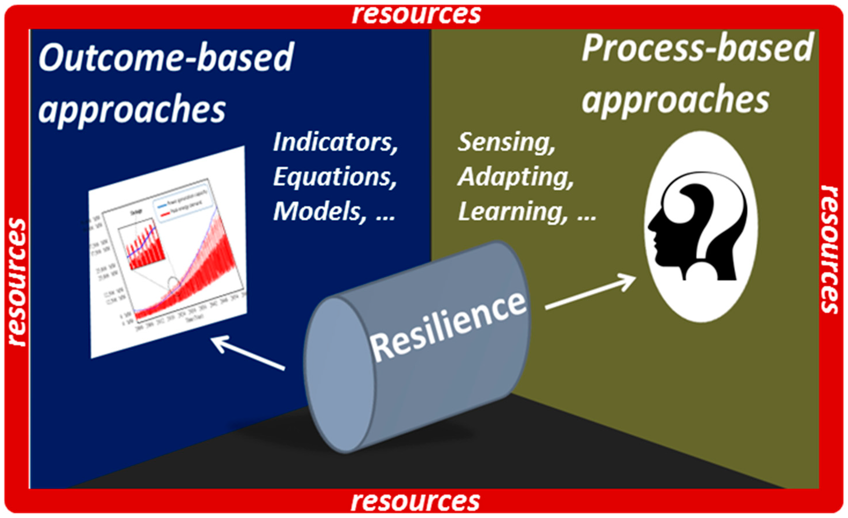
Figure 1. Integrated approach of resilience. Resilience approaches may be based on outcome- or process-based approaches under resources constraints. The purpose is to nest process-based approaches into outcome-based approaches under resources constraints in order to have an integrated view of resilience that fits both approaches.
Infrastructures 03 00011 g001
Figure 2. Outcome-based approach. This approach is based on a dynamical controlled system framework. According to the state of the system and management objectives, control u is decided. This framework enables managers to classify outcomes, including state variables, criteria, control, exogenous drivers, and dynamics of the system.
Infrastructures 03 00011 g002
Figure 3. Combining process- and outcome-based approaches for analyzing infrastructure resilience.
Infrastructures 03 00011 g003
Figure 4. Causal loop diagram of the system.
Infrastructures 03 00011 g004
Figure 5. Regular management. Under the regular management, we can see that outages appear (mainly during the summer). An outage occurs when the peak energy (in red) demand is higher than the power generation capacity (in blue).
Infrastructures 03 00011 g005
Figure 6. Influence diagram of the power infrastructure. The infrastructure is subjected to exogenous drivers and can be partially controlled. Resources (R) shown represent both costs and budget. Resilience options shown are M: Monitoring; S: Sensing; An: Anticipating; Ad: Adapting; L: Learning; and R: Resources.
Infrastructures 03 00011 g006
Figure 7. Influence of the different processes on the total duration of outages. In (a), Sobol indices of the different processes are shown. Adaptation is the most influential process here, followed by the anticipation process. In our case, the second-order Sobol indices are very low, showing a low dependency of the processes. Influences of adaptation and monitoring are also represented around a normalized reference (more or less 20%). Results are confirmed in (b,c), from which we can see that total duration of outages clearly depend on adaptation.
Infrastructures 03 00011 g007
Figure 8. Influence of the different processes on the costs. (a) Sobol indices of the different processes. Adaptation (b) and monitoring (c) are the most influential process here, followed by the anticipation process.
Infrastructures 03 00011 g008aInfrastructures 03 00011 g008b
Table 1. Summary of the model parameters. Note that only constant values of the parameters are reported; when no value is reported, it means that it is a dynamic variable.
Model ParametersDescriptionVariable TypeReference ValuesUnit
Power generation capacityNameplate capacity of power plant and the transmission lines required to distribute the generated electricity.Stock6000 *MW
New power infrastructure New power infrastructure built per year.Flow0 *MW/year
WearingPhysical wearing and aging of the existing power infrastructure per year.Flow200 *MW/year
Disruptions due to extreme events Electric power generation loss due to extreme events per year.Flow327 *MW/year
(Invested capacity recovery rate)The recovery rate that the system commits to after a loss due to extreme events per year.Flow0 *MW/year
Perceived wearingThe perceived physical wearing in the terms of capacity.Auxiliary MW
Perception delayThe time required to perceive the amount of capacity loss due to wearing and aging.Look up0.352year
Monitoring frequencyFrequency of monitoring the actual power infrastructure.Auxiliary6times in a year
Desired internal reserve marginThe desired amount of additional power generation capacity of power infrastructure above the peak energy demand. Auxiliary15%
Desired power generation capacityDesired power generation capacity to maintain the service.Auxiliary200 *MW
Peak energy demandThe peak energy demand in a given year. This variable is a function of exogenous variables of population and temperature change. Peak energy demand is experienced in summer months. Auxiliary2549 *MW
Perceived peak energy demandThe perceived amount of peak energy demand.Auxiliary3000 *MW
Peak energy demand perception delayThe amount of time required to perceive the trend of the peak energy demand in past years.Auxiliary1years
DiscrepancyThe difference between desired power generation capacity and the actual power generation capacity.Auxiliary0 *MW
New power infrastructure orderThe amount of power generation capacity required to be built.Auxiliary0 *MW
Adaptation responseThe response time to actualize the new power infrastructure order.Auxiliary6years
Construction delayConstruction time required to build new power plant and transmission lines.Auxiliary10years
Experience This is dimensionless variable, indicating a score of experience as a function of learning behavior and number of outages experienced in past.Auxiliary0 *(-)
Learning behaviorA dimensionless variable ranges between 0, no learning; and 1, perfect learning. Auxiliary0.5(-)
Learning scoreA dimensionless variable, varies between 1 and 3. Indicates improvement in fixing take up to 1/3 and strength of infrastructure to disruptions due to extreme events up to 3 times. The minimum learning score of 1 indicates that there is no improvement in both fixing time and strength of infrastructure.Auxiliary1 *(-)
* Values are at t0. For more detail and for dynamic values please see Appendix A.
Table 2. Main dynamical connections between outcomes, processes and resources.
Process Outcomes (Relevant Components)ResourcesLink
MonitoringState variables x ( t ) :
Power generation capacity, wearing
Parameter:
Monitoring frequency
Cost of monitoring activities, equipment installationThe monitoring process decides variables to be monitored and the frequency of monitoring (in our case, the wearing of physical infrastructure).
SensingState variables x ( t ) :
Perceived wearing
Parameter:
Perception delay
Assumed negligible costs involved, but requires willingness to changeThe sensing process corresponds to how the wearing of the infrastructure is perceived. In our case, we use a smooth function calibrated by the perception delay.
AnticipationParameter:
Desired internal margin reserve
-Anticipation decides if we foresee extreme events through the increase of the margin in order to face such extreme event.
AdaptationControl u(t):
New power infrastructure order
Criteria c(t):
discrepancy
Parameter:
Adaptation response
Cost of building new infrastructureWe adapt the building of new infrastructure according to the criteria based on the peak demand. This new infrastructure leads to additional costs.
LearningExogenous drivers w(t):
Parameter:
Learning ability
Costs associated with Infrastructure repair and readiness for future impacts of extreme eventsAfter each event, reconstructions are faster: we assume that we learn from previous experience for improving repairing processes.
Fixing infrastructure requires resources.