Research on Effectiveness of Vehicle Driving Simulation System Based on Coupling Modeling of Driving Behavior and Psychology

Abstract

Driving simulation systems play a critical role in the “human-vehicle-road-environment” ecosystem of road traffic, where their effectiveness is fundamental for advancing scientific research. This study proposes a comprehensive evaluation framework for such systems, employing a Mul-Bayes-LSTM model to analyze multidimensional data encompassing drivers’ biopsychological and behavioral characteristics. The evaluation process integrates Bayesian hyperparameter optimization to enhance model performance, with rank correlation and R² as key indicators of model fit. The gray correlation analysis, integrated entropy method, and CRITIC analysis are utilized for weighting these indicators, ensuring robust assessment. The overall evaluation index is derived using entropy and CRITIC methods to provide a comprehensive measure of simulation effectiveness. The results from experimental validation indicate that driver-specific parameters obtained from the test simulator closely align with behavioral variables in risk scenarios, confirming the system’s applicability for research in traffic perception. The research results can evaluate the effectiveness of driving simulators based on the driver’s perception level, which has certain significance for promoting the development and application of driving simulation systems.

1. Introduction

The vehicle driving simulation system is an experimental equipment for the simulation research and development of automobile active safety performance based on the whole performance of a “human-vehicle-road-environment” closed-loop system with the support of electronic computer, hydraulic pressure and control technology (Chen, 2021) [1]. The vehicle driving simulation system can provide a safe environment for driving research, can conveniently and economically formulate research strategies related to driving behavior, and has the characteristics of a wide range of experimental conditions, regulation and conversion, and online processing and classified storage of experimental data. At present, it has been widely used in the research of vehicle intelligent control, road traffic facilities, intelligent traffic system, driver behavior characteristic evaluation, self-driving and so on for the purpose of improving safety. For example, Min-Wook Kang et al. utilized a driving simulator to assess the impact of auditory warning sounds on driver compliance with roadside safety signs, revealing that compliance significantly increased when AWS was present (Min-Wook Kang et al., 2018) [2]. Although driving simulators are frequently used in studies, there is relatively little evidence to confirm their effectiveness, that is, how accurately they represent or reproduce real-world driving (Wynne et al., 2019) [3]. The vehicle driving simulation system offers an artificial virtual environment. In addition, if the risk conflict scenarios designed in this study were conducted directly in real-road vehicle experiments, they could involve high safety risks and road test approval restrictions. Therefore, this study opts to create controlled conflict scenarios in a driving simulator, aiming to assess the simulator’s ability to replicate drivers’ human factor responses under safe, controllable, and repeatable conditions. The experimental results may be affected by various factors, such as the scientific nature of the experimental goal conception, the rationality of the content selection, the representativeness of the sample (subjects) selection, the accuracy of the scenario design, and the realism of the humanoid perception. Therefore, evaluating driving simulation systems can provide new research ideas and directions for simulation systems. This is crucial for enhancing the usability of driving simulation systems and promoting their intelligent development.

To more clearly illustrate the relationship between existing research and the research gap in this paper, the study of the effectiveness of driving simulators is summarized into three stages: physical validity, behavioral validity, and human factor response validity. The first stage mainly focuses on the physical validity of the simulator, with the core issue being whether the simulator’s hardware system, vehicle dynamics, motion feedback, visual display, and control interface can closely approximate real vehicles and real-road environments. At the beginning of the development of driving simulation systems, validity research focused on analyzing the absolute performance differences between the simulation system and the real vehicle, i.e., basic validity (Wang et al., 2009) [4]. With the improvement of virtual scenario technology and more accurate vehicle-dynamic imitation operations in the model vehicle, the application of driving simulation systems gradually expanded to driving behavior and other research areas with higher requirements for experimental testing, and validity research also focused more on relative validity, behavioral consistency and other indicators, for which statistical tests are the main method for verifying validity (Groeger and Murphy, 2020) [5]. For example, Groeger completed the validity calibration of a simulator in 2019 by analyzing the parameters of driving behavior characteristics such as vehicle speed, braking, reaction time, and decision execution rate in real and virtual scenarios (Groeger and Murphy, 2020) [5]. The current validity evaluation of simulation systems is more based on the validity evaluation of driving behavior in integrated traffic scenarios (Hussain et al., 2019) [6]. Wang Junzheng et al. [7]. proposed an acceleration control-based physical simulation washout algorithm, which can significantly improve the dynamic fidelity of the driving simulator. Overall, research on physical validity provides an important basis for verifying the fundamental performance of driving simulators, but it mainly focuses on device performance, motion feedback, and scene realism, while paying insufficient attention to drivers’ behavioral responses and physiological and psychological changes in complex risk scenarios.

The research focus of the second stage gradually shifts from realism at the equipment level to the effectiveness of driving behavior. This stage mainly evaluates whether drivers’ explicit behaviors are consistent in the two environments by comparing indicators such as vehicle speed, acceleration, braking response, reaction time, lane position, trajectory deviation, and compliance with stopping in simulated environments and real-road environments. Zoeller selected time interval parameters to evaluate the effectiveness of the simulator by studying the braking behavior of vehicles crossing intersections under real and simulated conditions (Zoeller et al., 2017) [8]. Zhang Yanning et al. designed real vehicle and driving simulation experiments to verify the effectiveness of driving simulation techniques in a study of following speed (Zhang et al., 2020) [9]. Pawar et al. developed a generalized linear mixture (GLM) model to explore the behavioral (absolute and relative) validity of fixed-base driving simulators by conducting a comparative analysis of different driving behaviors (Pawar et al., 2022) [10]. Llopis-Castello et al. arranged volunteers to drive through the same section built by the self-developed simulator (SE2RCO) and selected 79 curves and 52 tangents of speed data for analysis (Llopis-Castelló et al., 2016) [11]. The objective validity of the simulator based on the average and working speeds was ensured by comparing the actual and simulated speeds. Cao et al. confirmed the reliability of driving simulators for driver behavior analysis at urban underpass entrances by continuously recording the speed of real car tests and driving simulator test feature points using two-factor variance analysis (Cao et al., 2015) [12]. In recent years, driving simulators have gradually been applied to studies of more complex road and infrastructure scenarios, such as underground interchanges, rural road curves, road markings, and traffic safety facility evaluations. Liu et al. used driving simulators and data mining methods to analyze the impact of traffic safety facilities at underground interchanges on driving safety and comfort; Martin-Castresana et al. [13]. investigated the effect of different road markings on speed control on rural road curves using driving simulators; and Bosurgi et al. proposed new behavioral evaluation indicators from the perspective of drivers’ steering behavior on curves. Tessa et al. verified the validity of a driving simulator with a mobile motion platform by comparing the analysis of motion sickness symptoms in real and virtual driving scenarios (Talsma et al.,2023) [14]. Larue et al. monitored driver behavior at passive level crossings in the Brisbane area of Australia for three months. They replicated the level crossing in an advanced driving simulator and established the relative effectiveness of stopping compliance and approach speed, validating the effectiveness of the driving simulator through comparison (Larue et al., 2018) [15]. Zhao Zhiguo verified the validity of the driving simulator data by collecting driving behavior data under different radius steering, regular lane change and emergency collision avoidance steering conditions and clustering the data using an improved K-means clustering method (Zhao et al., 2020) [16]. Overall, research on behavioral validity can fairly well evaluate a simulator’s ability to replicate driving behaviors, but the focus of such evaluations still mainly concentrates on observable behavior aspects such as speed, braking, reaction time, and trajectory, making it difficult to comprehensively reflect the driver’s psychological tension, risk perception, and physiological arousal in risky scenarios.

The third stage begins to focus on drivers’ human factor responses in risky traffic environments. With the development of human factor engineering and intelligent transportation research, merely analyzing overt driving behavior is no longer sufficient to fully explain the internal state of drivers. Therefore, physiological and psychological indicators have gradually been introduced into driving behavior analysis and the effectiveness evaluation of driving simulators. Napcil et al. evaluated the validity of the driving simulator by analyzing and comparing bicep surface EMG signals in steering behavior (Nacpil et al., 2020, 2021) [17,18]. Healey and Picard [19] collected physiological signals such as ECG, EMG, skin conductance, and respiration during real driving tasks to identify levels of driving stress. Nacpil evaluated the validity of driving simulator data by analyzing surface EMG signals during the steering process, In addition, Kierzkowski et al. [20]. involved eye movement and skin conductance response analysis in tram simulator studies, reflecting the development trend of human factor data collection in simulator research. Paliotto and Meocci [21] also developed road safety evaluation procedures from a human factors perspective, illustrating the importance of human factors in road safety assessment. Ghulam et al. [22] used a driving simulator to analyze the effects of vehicle-mounted attenuator markings on young drivers in work zones. Bella [23] validated the applicability of driving simulators in speed-related research from the perspectives of continuous speed profiles and speed behavior on two-lane rural roads, respectively. Liu et al. [24] combined a driving simulator with data mining methods to evaluate driving safety at underground interchanges, while Bosurgi et al. [25]. further extended the application of simulators to human–machine interaction and driving behavior analysis from the perspectives of simulator console design and steering behavior on curves. Overall, existing studies have provided a foundation for applying driving simulators to traffic safety and driving behavior analysis. However, a systematic simulator effectiveness evaluation framework that integrates driving behavior, biopsychological responses, and comprehensive evaluation methods is still lacking. Overall, behavioral validity research can effectively evaluate the simulator’s ability to replicate driving behaviors, but it is difficult to fully capture the psychological stress, risk perception, and physiological arousal processes of drivers in risky scenarios. Existing studies mostly focus on a single physiological signal or specific driving scenarios and still lack a systematic framework that integrates driving behavior, physiological and psychological responses, machine learning modeling, and comprehensive weighted evaluation.

Based on the comprehensive analysis of the above research results, the effectiveness of driving simulators is mainly studied from the perspectives of absolute realism and relative behavioral validity. However, in the “human-vehicle-road-environment” system of road traffic, drivers play a dominant role as users of the road, operators of vehicles, and perceivers of the external environment. The current research on the effectiveness of simulators from the perspective of drivers is insufficient. With the development of human–machine ergonomics, biopsychological indicators of drivers are increasingly used to analyze driving behavior. Considering the nonlinearity and uncertainty of psychological parameters of drivers in simulator experiments, and the good nonlinear fitting and deep feature mining capabilities of deep learning models, this paper constructs a comprehensive evaluation model of simulators based on the biopsychological and behavioral characteristics of drivers using machine learning methods. The model input layer consists of variables of vehicle, road, and environmental features of the simulator, and the output layer is a two-dimensional feature matrix of human factors. Based on Bayesian hyperparameter optimization to better match the human factors, reflect the actual experimental effects of the simulator, and complete the comprehensive evaluation of the simulator based on weighted analysis, this paper explores the comprehensive effectiveness evaluation method of automobile driving simulators based on human factors. This paper constructs a Mul-Bayes-LSTM evaluation model, taking vehicle, road, and conflict scene parameters as inputs, and EDA, ECG, and EMG as outputs, aiming to extract the correlation features between driving behavior and physiological–psychological responses, and to evaluate the effectiveness of the driving simulator.

2. Designing Comprehensive Evaluation Experiment Scene

This chapter mainly introduces the driving simulation experimental platform, the design of traffic conflict scenarios, data collection methods, and the selection criteria for experimental subjects. To ensure the comparability of the experimental results, this study constructs a standardized unsignalized intersection conflict scenario and simultaneously collects vehicle operation parameters and drivers’ physiological and psychological data, providing a foundation for subsequent model development.

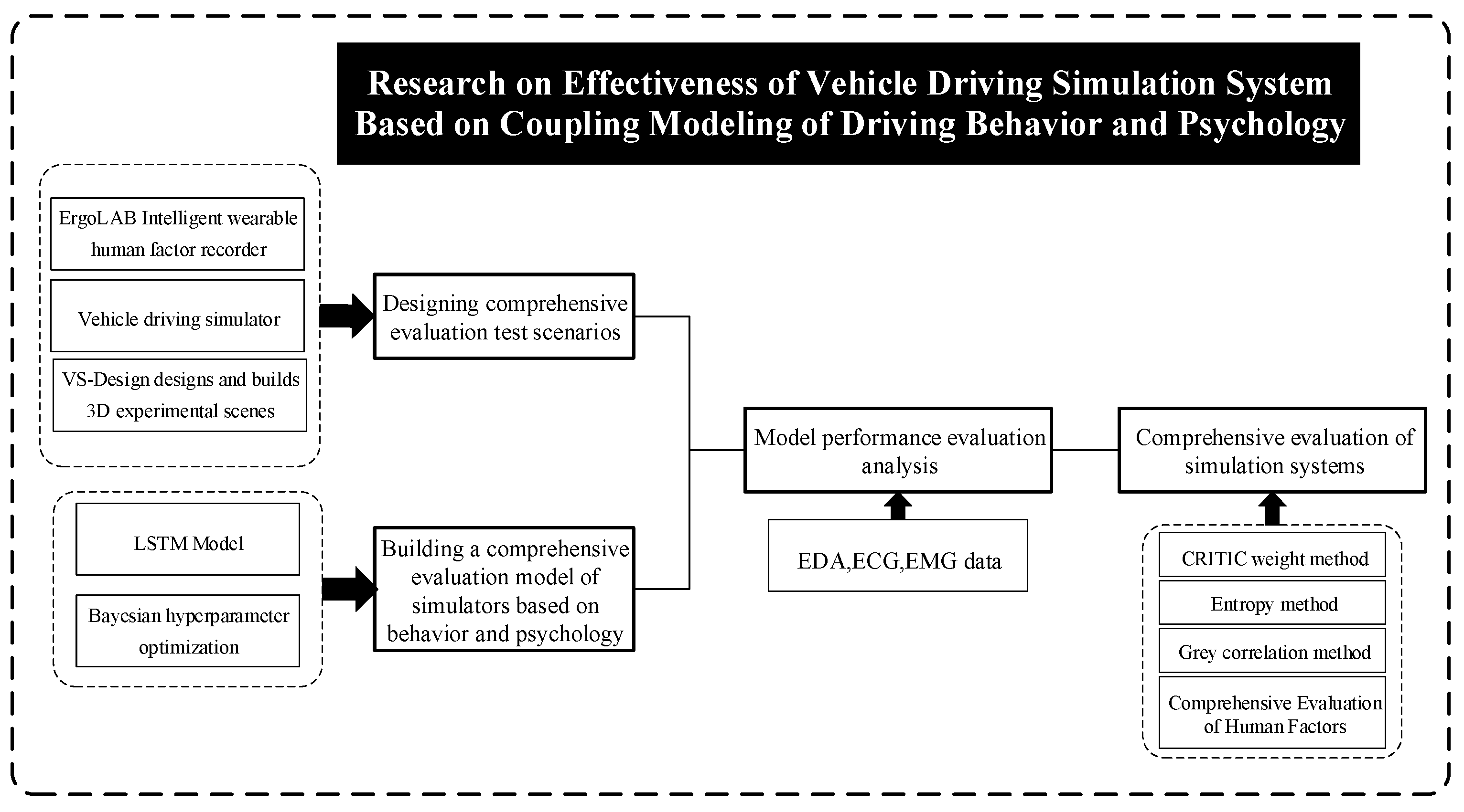
The technical route of this paper is as shown in Figure 1.

2.1. Experiment Equipment and Scene Design

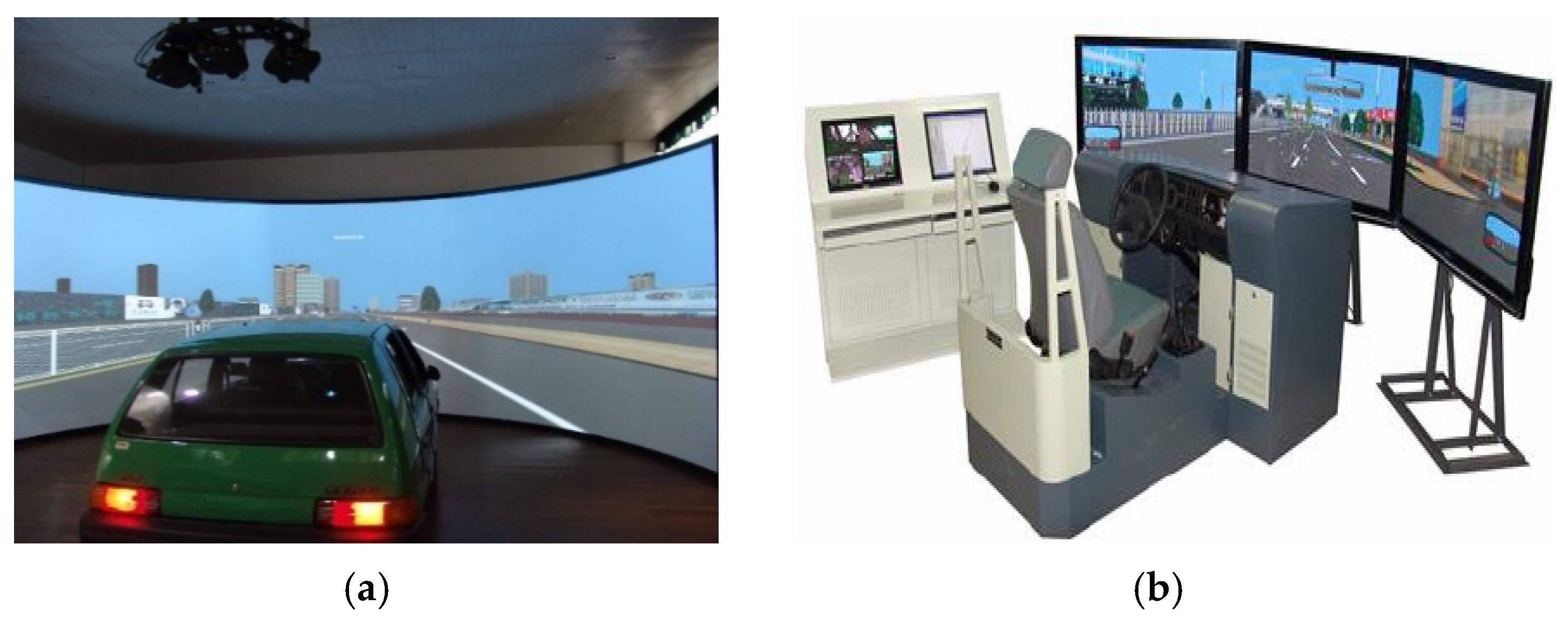
The simulator used for the experiments is shown in Figure 2. It adopts a split-type three-screen display device and is equipped with the VehicleModel2.0 vehicle dynamics model. The construction of the virtual road environment scene is realized through the laboratory’s self-developed software VS-Design. This article uses lab-developed interactive visualization scene generation software. The system uses OpenGL for real-time interaction and is programmed with Visual C 6.0, solving the issue of real-time interaction in virtual scenes while allowing quick generation and modification of virtual scenes. The VehicleModel2.0 allows this simulator to provide living driving experience and related data. The simulator cockpit has two types: a real car driving cabin and a self-built one. Using them for driving simulator effectiveness experiments has a certain representativeness.

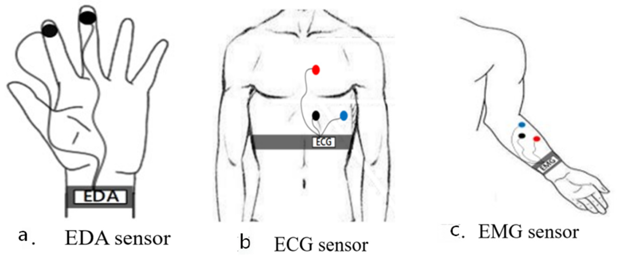
The driver’s biopsychological data was collected through an ErgoLAB physiological instrument as shown in Figure 3. The ErgoLAB EXG is a wearable wireless human factor physiological recording device. It’s the second-generation physiological recording device independently developed by Beijing Jinfatai Technology Co., Ltd. in Beijing, China. The experimental data include: main vehicle speed and displacement, acceleration, brake pedal depth and other operational characteristic data, as well as the speed and displacement data of the conflict vehicle; and ErgoLAB-physiological-instrument-collected electrodermal activity (EDA), electromyography (EMG), electrocardiogram (ECG) and other physiological characteristic data.

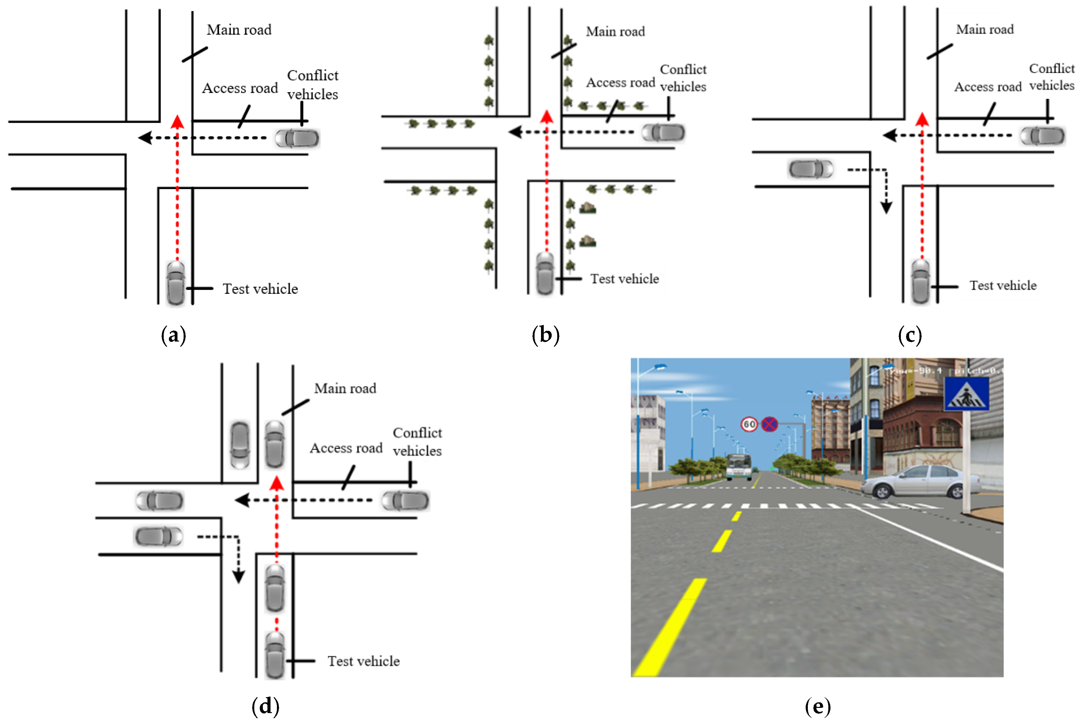
The experiment used the self-developed VS-Design software to design and construct virtual 3D experimental scenes, to highlight the psychological characteristics of drivers and study their driving behavior in conflict situations. The experimental scenes were designed as shown in Figure 4, including head-on collisions between motor vehicles at unsignalized intersections with no obstruction, with obstruction, with low traffic flow, and with heavy traffic flow. According to the Chinese urban road and intersection design specifications, the lane width of the experimental scene was designed to be 3.5 m, and external factors such as weather were excluded to minimize their impact on driving behavior. The traffic conflict was triggered by setting a trigger zone. The main vehicle traveled from south to north through the intersection, while the conflicting vehicle A traveled from east to west at a speed of 40 km/h and collided with the main vehicle perpendicularly. If there was a conflicting vehicle B, it entered the intersection from the west and turned right at a speed of 30 km/h. All these scenarios were simulated in the driving simulator.

The speed parameters of conflicting vehicles mainly refer to the relevant requirements for urban road and intersection operating speeds in the “Urban Road Design Code” (CJJ 37-2012) and the “Urban Road Intersection Design Specifications” (CJJ 152-2010), and are set in conjunction with the unsignalized intersection conflict scenarios constructed in this study. A fixed speed is used herein primarily to ensure that different participants are exposed to consistent experimental stimuli, thereby improving experimental repeatability and data comparability. In subsequent studies, the speed of conflicting vehicles can be set to dynamic variations such as acceleration, deceleration, or random disturbances according to the research objectives.

2.2. Experimental Participants

To avoid interference from other factors, drivers with skilled driving skills and more than three years of driving experience with a mileage exceeding 20,000 km were selected as testers. The tester’s physical health did not include any diseases that would affect the driver’s biopsychology, and the driver had experience in simulator operation. The experiment brought together 27 testers, including nine female participants. The age range of the test subjects was 21–56 years, with an average age of 34.74 years and a standard deviation of 9.65 years, covering drivers from youth to middle age. For details on the subjects’ gender, driving experience, driving mileage, accident history, and violations, see

Table 1. Driver detailed information.

Driver No.	Gender	Driving Experience/Mileage	Age	Accident in the Past Three Years (Y/N)	Traffic Violation in the Past Three Years (Y/N)
1	Female	9 years/50,000–60,000 km	35	N	N
2	Male	24 years/250,000 km	56	N	Y
3	Male	9 years/100,000 km	38	N	Y
4	Male	9 years/100,000 km	38	N	N
5	Male	10 years/80,000 km	43	N	Y
6	Male	4 years/30,000 km	28	N	Y
7	Male	8 years/140,000 km	41	Y	Y
8	Female	7 years/10,000 km	41	N	N
9	Female	10 years/50,000 km	38	N	N
10	Male	24 years/200,000 km	46	N	Y
11	Female	8 years/70,000 km	39	N	Y
12	Female	6 years/50,000 km	48	N	Y
13	Female	12 years/100,000 km	39	N	Y
14	Female	5 years/50,000 km	32	N	N
15	Female	14 years/60,000 km	33	N	Y
16	Female	14 years/60,000 km	38	N	Y
17	Male	15 years/150,000 km	37	N	Y
18	Male	5 years/60,000 km	24	N	N
19	Male	4 years/100,000 km	23	N	N
20	Male	3 years/10,000 km	23	N	N
21	Male	20 years/300,000 km	51	N	N
22	Male	3 years/50,000 km	33	N	N
23	Male	4 years/50,000 km	23	N	Y
24	Male	3 years/20,000 km	24	N	N
25	Male	3 years/20,000 km	24	N	N
26	Male	4 years/80,000 km	22	N	N
27	Male	3 years/20,000 km	21	N	N

.

The design time of the experiment is about 25 s from driving into the conflict section to driving out of the conflict intersection completely. To ensure that the human factor parameters can be identified in a timely and efficient manner, the statistical interval of the experiment data is set to 0.2 s. At the same time, to avoid interference caused by driving fatigue caused by complex scenes, the experiment time is set to about 10 min, and the experimental mileage is set to about 10 km.

Although the current sample size is sufficient to support preliminary validation of the proposed Mul-Bayes-LSTM framework under controlled simulator conditions, it may still limit the model’s generalizability to a broader driver population. Differences in age, driving experience, risk preference, and driving style may result in varying behaviors and psychophysiological responses. To mitigate the impact of the limited sample size, this study employed standardized experimental scenarios, unified data collection procedures, and K-fold cross-validation. Future work will further expand the participant sample and include a more diverse group of drivers to enhance the external applicability of the proposed framework.

3. Constructing Comprehensive Evaluation Model of Simulator Based on Behavior and Psychology

This chapter constructs a Mul-Bayes-LSTM evaluation model based on the coupling of driving behavior and physiological–psychological responses. The model takes vehicle operation parameters, road environment parameters, and conflict scenario parameters as inputs, and EDA, ECG, and EMG as outputs. It extracts attribute correlations and temporal dynamic features through CNN-LSTM, and uses Bayesian optimization to improve the efficiency of model parameter selection.

3.1. LSTM-Based Evaluation Model of Simulator Efficiency

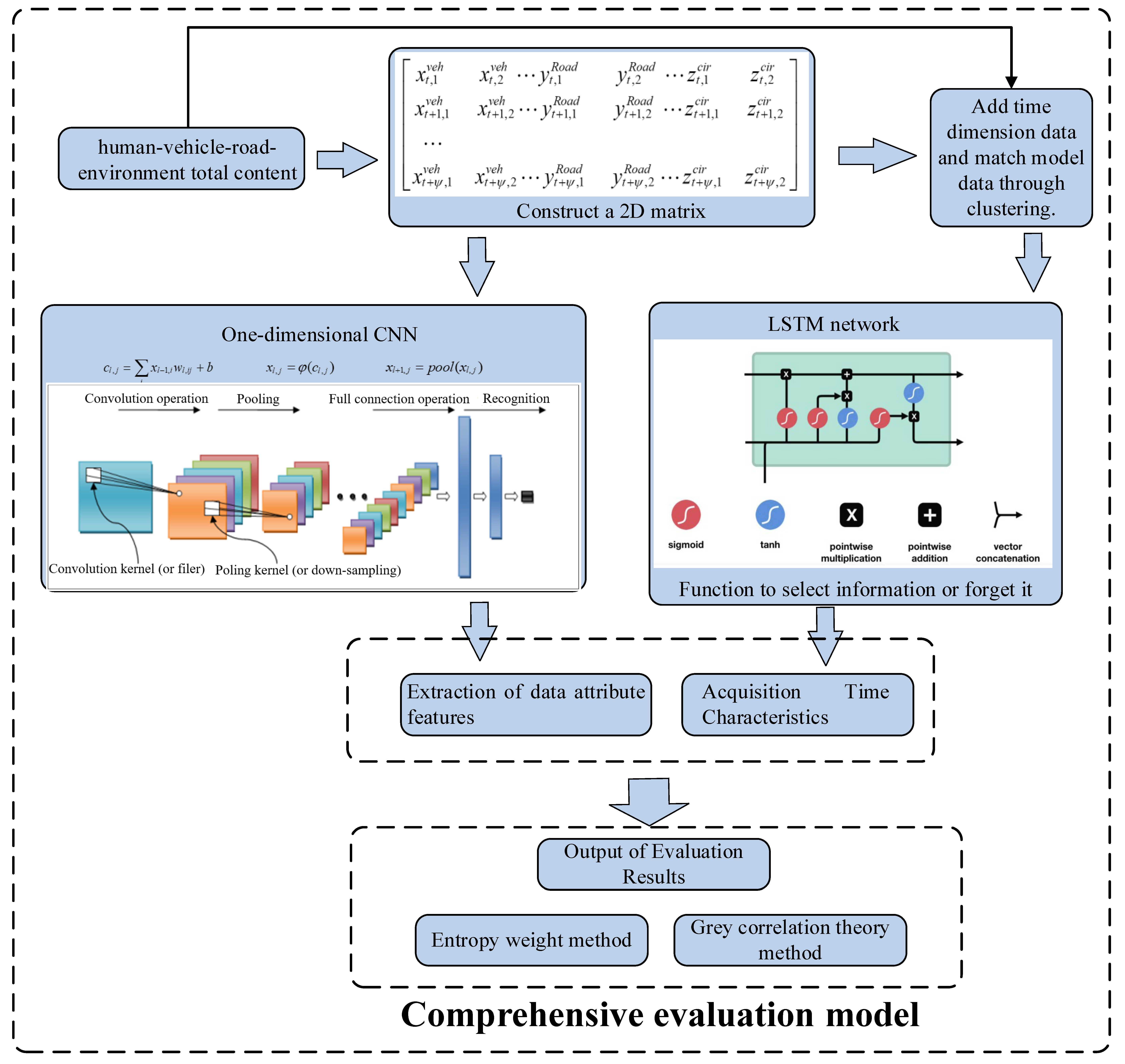
Traditional recurrent neural networks can handle time series data, but when dealing with longer time spans and complex sequence data, they are prone to issues such as insufficient capture of long-term dependencies, vanishing gradients, or exploding gradients. In driving simulation experiments, drivers’ behavioral responses and physiological–psychological responses exhibit obvious continuity and temporal dependence. The driving response at a certain moment is influenced not only by the current traffic conflict stimulus but also possibly by previous changes in speed, steering operations, braking behavior, and psychological arousal states. Therefore, it is necessary to use models with stronger temporal memory capabilities to model driving behavior and physiological–psychological data. The LSTM model has good performance for multi-attribute data processing; for example, Li Siteng et al. proposed three hybrid deep learning models combining multi-factor external and internal features to predict online car-hailing (OCH) demand, and long short-term memory (LSTM), bidirectional LSTM (BiLSTM), gated recurrent unit (GRU), and convolutional LSTM (ConvLSTM) were selected to extract features (Li et al., 2023) [26]. Therefore, this paper proposes an ensemble machine learning method based on the LSTM model, which is better suited for evaluating high-dimensional and multi-attribute driving simulators. To collect and process the full range of “human-vehicle-road-environment” data, a two-dimensional feature matrix containing time-state information is constructed. This matrix is then input into the model to extract matching human factor features, and the model’s evaluation effect is obtained. The comprehensive evaluation model is formed by applying the entropy weight method and gray correlation theory to analyze the evaluation results with comprehensive weights. The method process is illustrated in Figure 5.

3.2. CNN-LSTM Feature Extraction and Tuning Hyperparameters with Bayesian

3.2.1. Construct Characteristic Matrix

Given the time-varying traffic flow in the experimental scenario, and the fact that the evaluation index of the experiment is the operational effectiveness of the simulator, this paper constructs a two-dimensional feature matrix that contains spatio-temporal “parameter-evaluation” information. The matrix is represented by Formula (1):

$$\left[{\displaystyle \genfrac{}{}{0pt}{}{x_{t,1}^{veh} x_{t,2}^{veh} ... y_{t,1}^{Road} y_{t,2}^{Road} ... z_{t,1}^{Cir} z_{t,2}^{Cir}}{\begin{array}{c}{x}_{t+1,1}^{veh} x_{t+1,2}^{veh} ... y_{t\_1,1}^{Road} y_{t+1,2}^{Road} ... z_{t+1,1}^{Cir} z_{t+1,2}^{Cir}\\ ... \\ x_{t+\psi ,1}^{veh} x_{t+\psi ,2}^{veh} ... y_{t+\psi ,1}^{Road} y_{t+\psi ,2}^{Road} ... z_{t+\psi ,1}^{Cir} z_{t+\psi ,2}^{Cir}\end{array}}}\right]$$

(1)

In the formula, $x_{t,1}^{veh}$ and $x_{t,2}^{veh}$ represent the parameters of the first and second types of vehicles collected at different times, $y_{t,1}^{Road}$ and $y_{t,2}^{Road}$ represent the road characteristic parameters of the first and second types, and $z_{t,1}^{Cir}$ and $z_{t,2}^{Cir}$ represent the environmental characteristic parameters of the first and second types.

CNNs are mainly composed of convolutional layers, pooling layers, and fully connected layers, with the descriptions of the three layers shown in Formulas (2) and (3):

$$C_{l,j}=\sum x_{l-1,i}{w}_{l,ij}+b$$

(2)

$$x_{l+1,j}=pool\left(x_{l,j}\right)$$

(3)

In the equation, $x_{l-1,i}$ is the input of the convolutional layer; $x_{l-1,i}$ is the output of the convolutional layer, which is the input of the activation layer; $x_{l,j}$ is the output of the activation layer; $w_{l,ij}$ is the weight between the l-th layer’s nth unit and the i-th unit of the previous layer; $b$ is the bias term; ${\phi }_c$ is a nonlinear activation function; and $pool\left(x\right)$ is the pooling function. Simulator data has characteristics such as randomness and time-variability. After constructing the feature matrix, the feature matrix is input into the CNN to successively extract the attribute features of the data, that is, horizontally traversing the two-dimensional feature matrix. After using CNN to extract data attribute features, it is necessary to extract temporal features; the paper uses an LSTM network to capture temporal features, that is, vertically traversing the two-dimensional feature matrix.

Simulator data exhibits randomness and temporal variability. Therefore, the feature matrix is constructed and input into a Convolutional Neural Network (CNN) to sequentially extract attribute characteristics of the data. This involves traversing the two-dimensional feature matrix horizontally. After extracting data attribute features using CNN, time features are extracted using an LSTM network. This involves longitudinally traversing the two-dimensional feature matrix. The obtained data are then reduced using stepwise regression. Next, 80% of the sample data is randomly selected as the training set, while 20% is used as the test set and input into the simulator evaluation model. The test set is used only for final evaluation and does not participate in model training or hyperparameter selection. Considering the relatively limited sample size, this paper further uses the K-fold cross-validation method to perform supplementary testing of model stability, in order to reduce the impact of a single random split on the model evaluation results.

3.2.2. Model Optimization

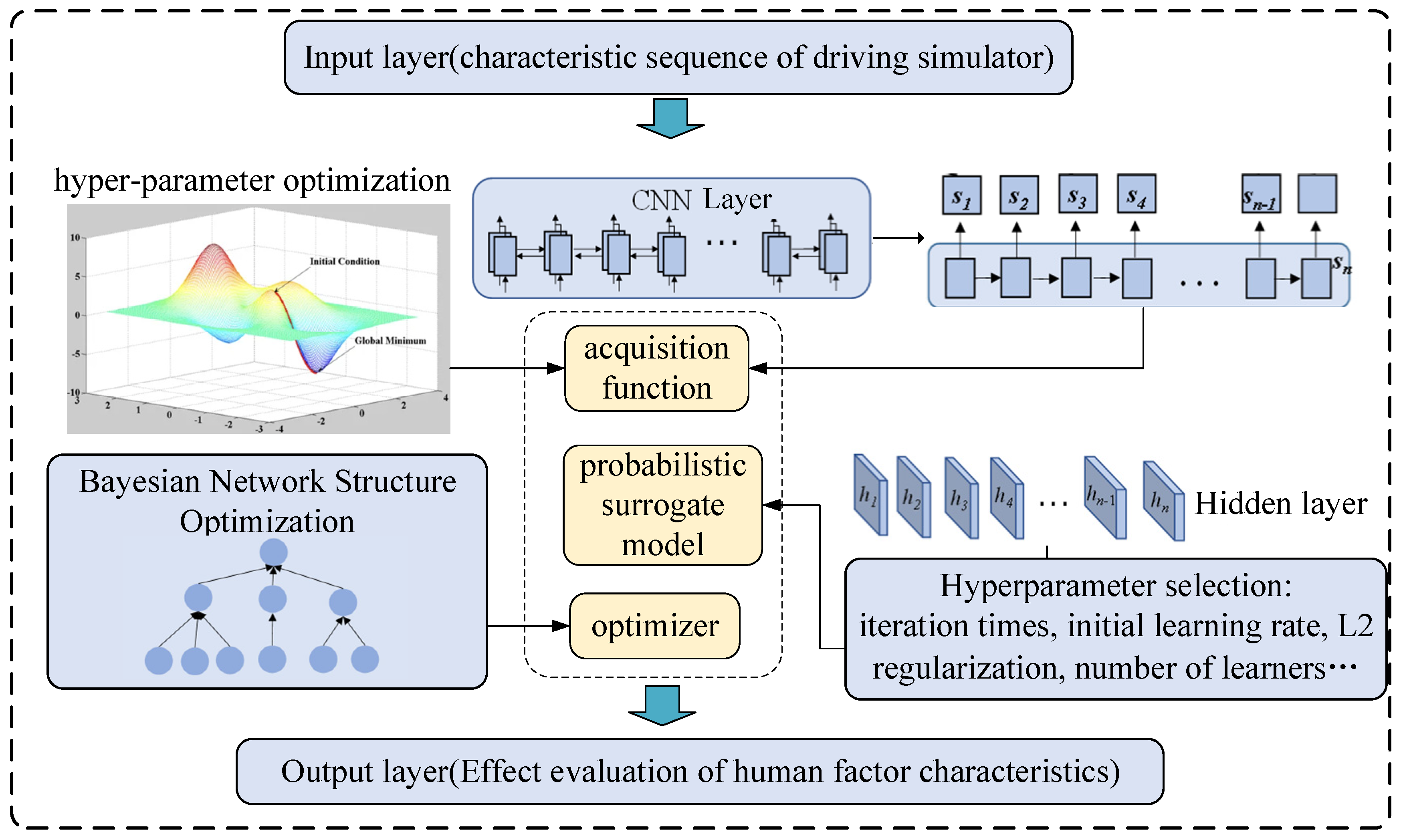
The training process utilizes the Adam iterative optimization algorithm to dynamically adjust the learning rate of each parameter by estimating the first-order and second-order moments of the gradient. L2 regularization is applied to optimize the weight parameters of the LSTM model and prevent overfitting. Due to the lengthy training time of LSTM, manually setting the training parameters can significantly impact prediction performance. Currently, commonly used hyperparameter tuning methods such as grid search involve a global search with a large search range and small step size, which is computationally intensive. Random search can easily lead to local optima. Bayesian optimization, which uses a Gaussian process to consider previous parameter information and has the characteristics of fewer iterations and faster operation, can effectively search the hyperparameter space. Therefore, this thesis adopts Bayesian optimization for hyperparameter tuning of LSTM models. The Bayesian hyperparameter optimization algorithm consists of a probabilistic agent model and a collection function, as shown in Figure 6. The flow is as follows:

• In probability-based agent models, Gaussian processes are used as prior functions, which can be represented as:

$$f~gp\left(m\left(x\right),k\left(x,x^{\prime }\right)\right)$$

(4)

In the formula, $m\left(x\right)$ is the mean velocity function, and $k\left(x,x^{\prime }\right)$ is the velocity covariance function. Taking the normalized electromyography (EMG) parameters as an example, assuming the sample points of EMG data as $D=\left(x_{1:t},y_{1:y}\right)$, and its covariance matrix is denoted as:

$$\mathrm{K}=\left[\begin{array}{c}k\left(x_1,x_1\right) k\left(x_1,x_2\right)... k\left(x_1,x_t\right)\\ k\left(x_2,x_1\right) k\left(x_2,x_2\right)... k\left(x_2,x_t\right)\\ ... ... ...\\ k\left(x_t,x_1\right) k\left(x_t,x_2\right)... k\left(x_t,x_t\right)\end{array}\right]$$

(5)

With the addition of new EMG data sample D, the covariance matrix is updated as shown in formula:

$$K=\left(\begin{array}{c}K k^T\\ k k\left(x_{t+1},x_{t+1}\right)\end{array}\right)$$

(6)

where the posterior probability distribution of $k=\left[k\left(x_{t+1},x_1\right),k\left(x_{t+1},x_2\right),...,k\left(x_{t+1},x_t\right)\right]$ is calculated from the previous $t$ EMG data samples as shown in the formula:

$$P\left(f_{t+1}|D_{1:t},x_{t+1}\right)~N\left(\mu ,{\sigma }^2\right)$$

(7)

$${\sigma }^2=k\left(x_{t+1},x_{t+1}\right)-K^T{K}^{-1}k$$

(8)

$$\mu =k^T{K}^{-1}{f}_{1:t}$$

(9)

According to the above formula, the normal distribution that follows at any value can be estimated, so the sampling function can be used to locate the next most “promising” sample point.

ii.

Using the classical $EI$ criterion as the acquisition function, which is shown in Formulas:

$$EI\left(x\right)=\left\{\begin{array}{c}\mu \left(x\right)-f\left(x^{+}\right)\Phi \left(Z\right)+\sigma \left(x\right)\varphi \left(Z\right) \sigma \left(x\right)>0\\ 0 \sigma \left(x\right)<0\end{array}\right.$$

(10)

$$Z={\displaystyle \frac{\mu \left(x\right)-f\left(x^{+}\right)}{\sigma \left(x\right)}}$$

(11)

where $\Phi \left(Z\right)$ is the probability density function of the standard normal distribution, and $\varphi \left(Z\right)$ is the distribution function of the standard normal distribution.

To improve the efficiency and stability of LSTM model hyperparameter selection, this paper employs Bayesian optimization to search for the model’s key parameters. Unlike grid search and random search, Bayesian optimization can leverage existing parameter combinations and their model error results, continuously update the surrogate model, and guide the next round of parameter selection.

Let the historical sample set that has been evaluated before the t-th iteration be:

$$D_t={\left\{\left({\theta }_i,L\left({\theta }_i\right)\right)\right\}}_{i=1}^t$$

(12)

Here, ${\mathsf{\theta }}_{\mathrm{i}}$ represents the i-th combination of hyperparameters, and $\mathrm{L}\left({\mathsf{\theta }}_{\mathrm{i}}\right)$ represents the model loss value or validation error corresponding to that set of parameters. The hyperparameters in this paper mainly include the number of LSTM hidden layer units, initial learning rate, L2 regularization coefficient, number of training iterations, and so on. The model optimization objective can be expressed as:

$$\theta *=arg \underset{\theta \in \Omega }{\mathit{min}} L\left(\theta \right)$$

(13)

Here, Ω represents the hyperparameter search space, and $\mathsf{\theta }*$ represents the optimal hyperparameter combination that minimizes the model error.

In each iteration, Bayesian optimization first builds or updates a Gaussian process surrogate model based on the historical sample set ${\mathrm{D}}_{\mathrm{t}}$:

$$f\left(\theta \right)~GP\left(m\left(\theta \right),k\left(\theta ,{\theta }^{\prime }\right)\right)$$

(14)

Here, $\mathrm{m}\left(\mathsf{\theta }\right)$ is the mean function, and $\mathrm{k}\left(\mathsf{\theta },{\mathsf{\theta }}^{\prime }\right)$ is the covariance function. This surrogate model is used to estimate the posterior distribution of the objective function values corresponding to different combinations of hyperparameters. Subsequently, the next set of candidate hyperparameters is selected using the expected improvement function:

$$EI\left(\theta \right)=E\left[max\left(f_{best}-f\left(\theta \right),0\right)\right]$$

(15)

$${\theta }_{t+1}=arg \underset{\theta \in \Omega }{\mathit{max}} EI\left(\theta \right)$$

(16)

Here, ${\mathrm{f}}_{\mathrm{b}\mathrm{e}\mathrm{s}\mathrm{t}}$ represents the optimal objective function value obtained from the current historical samples.

It can be seen that Bayesian optimization can use previous parameter combinations and their model errors as prior information, balancing the use of already good parameter regions and exploring uncertain parameter regions, thereby improving the efficiency of hyperparameter search.

During the model training process, the test set is only used for the final model performance evaluation and does not participate in hyperparameter selection. If a separate validation set is used, the validation set error is taken as Lθ; if the sample size is limited, the internal cross-validation error of the training set is used as Lθ, to reduce the impact of a single data split on optimization results. When the objective function value no longer decreases significantly after several consecutive iterations, the Bayesian optimization process is considered basically converged, and the currently optimal hyperparameter combination is taken as the final model parameters.

4. Evaluation Model Performance Analysis

This chapter analyzes the prediction performance and optimization effect of the Mul-Bayes-LSTM model. This paper selects indicators such as (R²), rank correlation, MSE, RMSE, NRMSE, ErrorMean, and ErrorStd to evaluate the model’s performance from the perspectives of fitting degree, correlation, and error distribution, and further explains the differences in EDA, ECG, and EMG results.

4.1. Model Effect Analysis

$R^2$ and rank correlation are used as indicators to judge the fitting degree of the intersection of predicted values and original values; Mean Squared Error (MSE), Root Mean Squared Error (RMSE), Normalized Root Mean Squared Error (NRMSE), Mean Absolute Error (ErrorMean), and Standard Deviation of Absolute Error (ErrorStD) are used as measurement indicators to judge the matching degree of the model. The statistical results of the model operation are shown in Table 1, and the model’s R², error comparison, rank correlation, and mean deviation are shown in

Table 2. The fitting value at the intersection of predicted value and original value.

	${\mathbf{R}}^2$	MSE	RMSE	NRMSE	Rank Correlation	Error Mean	Error Std
EMG	0.7122	212.2497	14.5688	−0.9109	0.7792	−1.8282	14.4826
ECG	0.9739	358.0546	18.9223	−0.3277	0.9054	−1.8729	18.8672
EDA	0.9662	0.0013	0.0360	0.0033	0.9775	−0.0046	0.0358

.

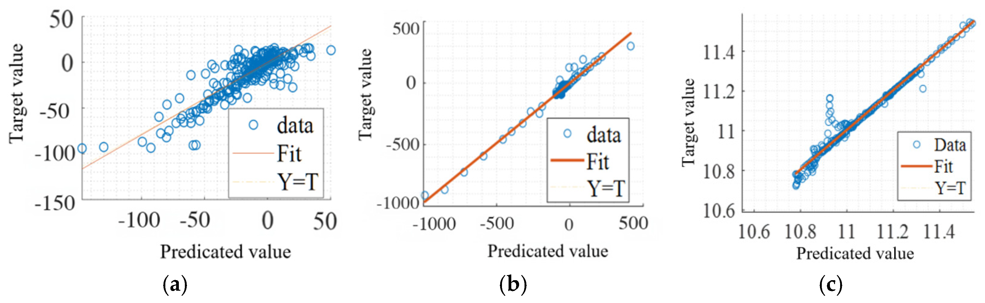
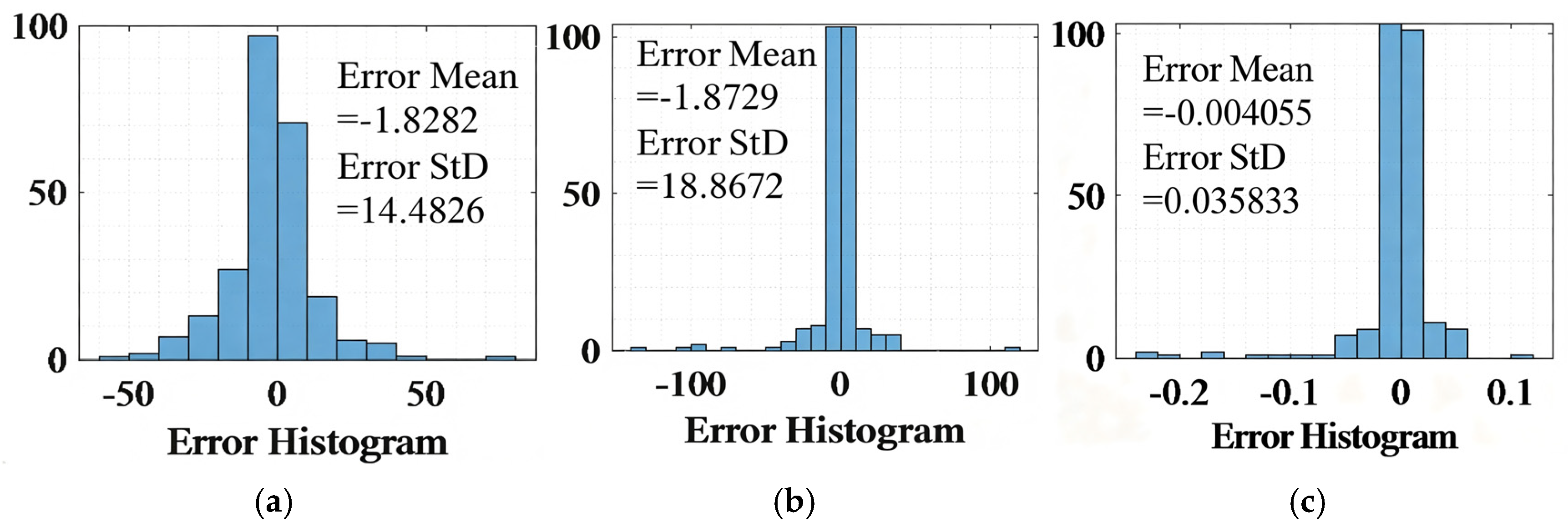
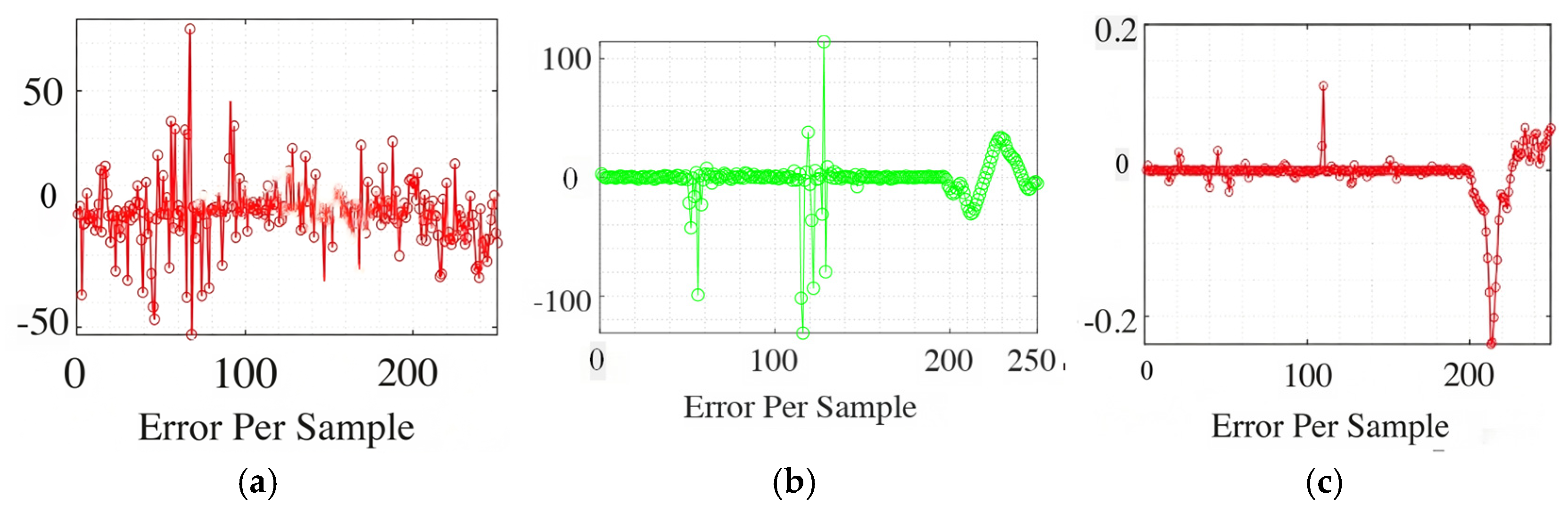
According to Figure 7 and Figure 8 the specific prediction results of the model are as follows: the R² value of EDA is 0.9662, the R² value of ECG is 0.9739, and the R² value of EMG is 0.7122. The specific features in the graph are: the intersection of the predicted values of EDA and ECG with the original values (blue circles) is relatively concentrated, so the degree of fit is high; the intersection of the predicted values of EMG with the original values (blue circles) is more discrete, resulting in a relatively low degree of fit. In contrast, the EDA predicted values have the smallest error values with respect to the original values. The distribution of EDA single-sample errors is the most stable and concentrated, with large error fluctuations mainly around the 210th–220th samples; meanwhile the ECG single-sample errors are more volatile than the EDA single-sample errors, resulting in larger overall errors; the EMG single-sample error distribution is relatively discrete, and the overall errors are relatively large. Comprehensive analysis of the above indicators found that the overall effect of the model is good and has a good fit.

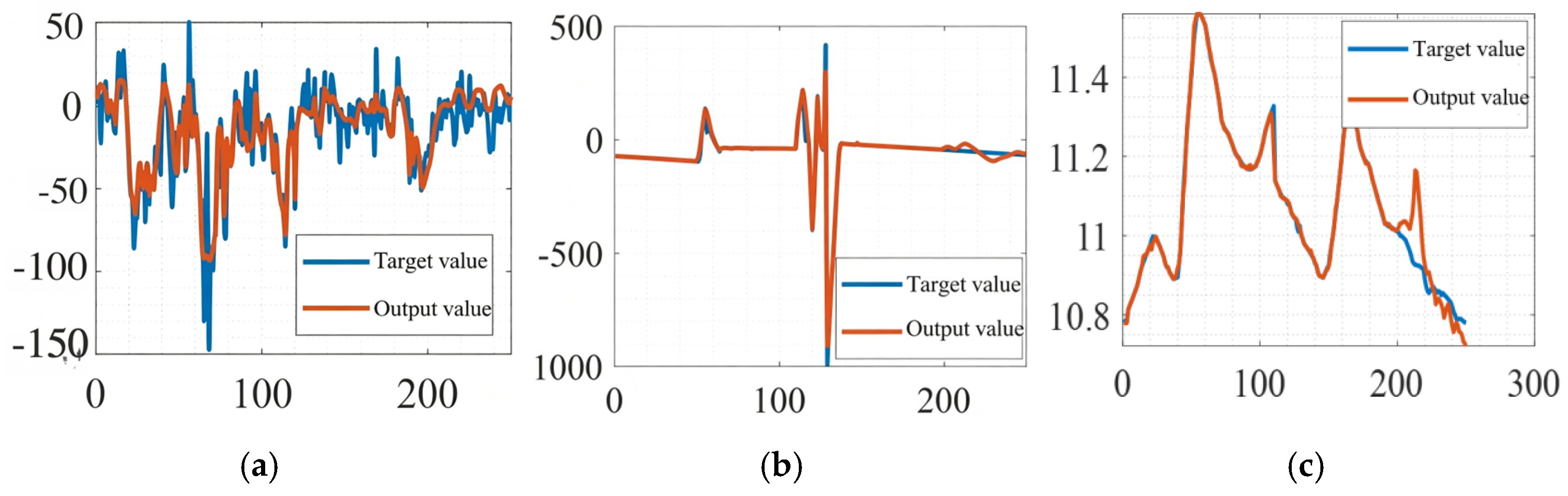
According to Figure 9 shows the time-series fitting curves of the target measured value and the model predicted output value under three different feature dimensions. It can be seen that the proposed Mul-Bayes-LSTM model can well track the fluctuation trend of the original human factor driving data, and only slight deviation exists at individual extreme mutation points, which preliminarily verifies the strong time-series feature learning ability of the model. According to Figure 10 The model prediction results show that the fitting performance of EDA and ECG is better than that of EMG, which is mainly related to the stability and sensitive characteristics of different physiological signals. EDA is closely related to emotional arousal, psychological tension, and risk perception, and changes more noticeably in traffic conflict scenarios; ECG can reflect cardiovascular responses under psychological load and driving stress, with an overall relatively stable trend. In comparison, EMG is more easily affected by factors such as grip strength on the steering wheel, arm posture, pedal operation, sensor attachment position, and individual driving habits, leading to greater short-term fluctuations and noise, and therefore the model fitting effect is relatively weak. This indicates that EMG is more suitable as an auxiliary indicator in the evaluation of driving simulator effectiveness.

4.2. Optimization Effect Analysis

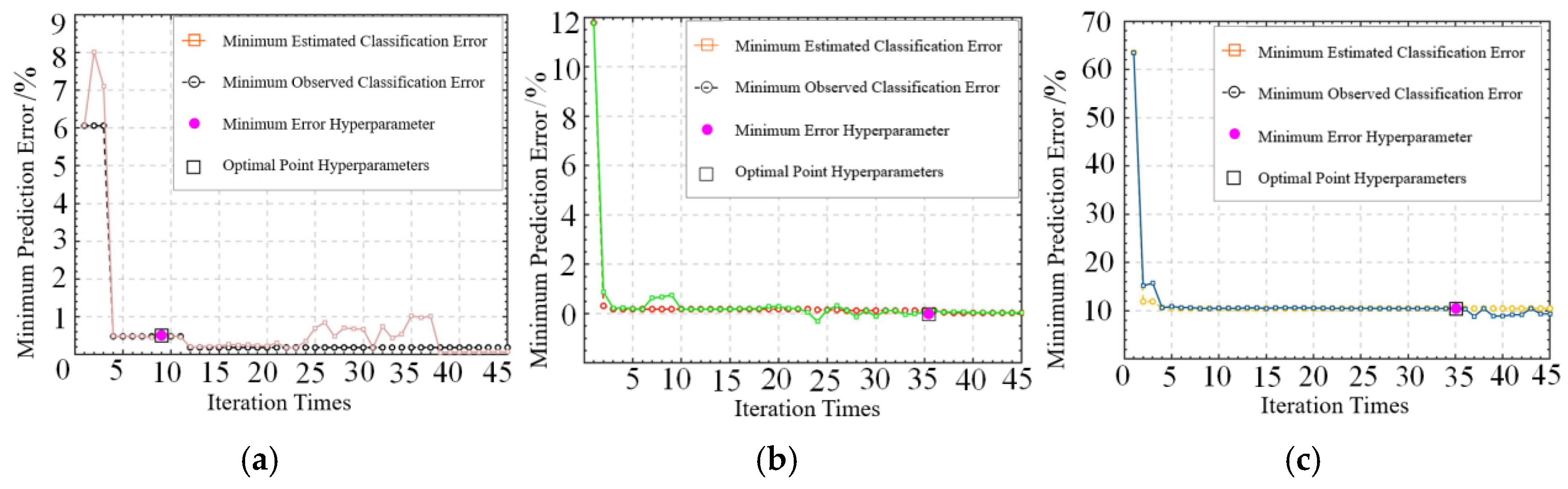
As shown in Figure 11, when the Bayesian superparametric optimizer iterates to the fourth, second and second times respectively for EDA, ECG and HEV data, the prediction error is sharply reduced by about 8%, 11%, and 53%; when iterating to the ninth, 36th and 35th times, the minimum error and the best point super parameter are obtained. At this time, the model converges, indicating that Bayesian optimization can be used in the task of high-cost evaluation of objective function. If the super parameter can converge rapidly in the iteration, it can be effectively applied to the evaluation of driving simulation scenarios. To further verify the adaptability of the simulator data, a K-fold cross-validation method is adopted to evaluate the effectiveness of the model. Each subsample participates in training and testing, which can reduce the generalization error. Figure 11. Bayesian hyperparameter optimization iteration curves of three groups of feature datasets. The hollow square line represents the minimum estimated classification error (orange in subgraph (a), green in subgraph (b), blue in subgraph (c)), and the hollow circle dashed line denotes the minimum observed classification error (black in subgraph (a), red in subgraph (b), yellow in subgraph (c)). The fuchsia solid dot marks the iteration with the minimum error, and the hollow square indicates the optimal hyperparameter point.

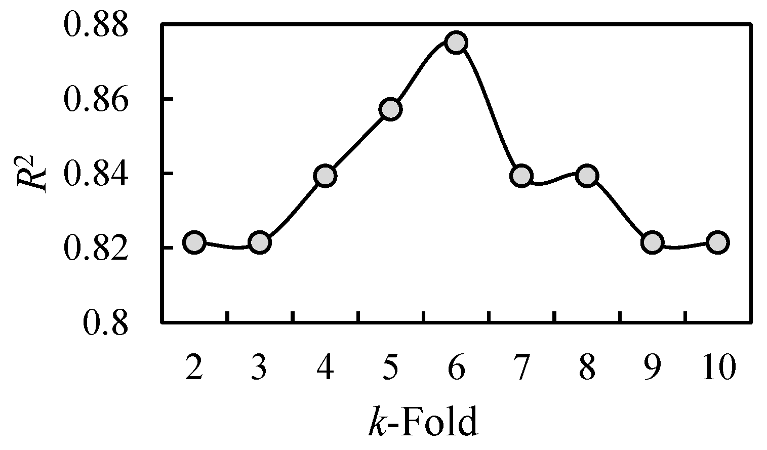
To further verify the adaptability of the Mul-Bayes-LSTM model to driving simulator data, this study sets K = 2 to K = 10 for cross-validation and calculates the R² values under different folds to analyze model stability and overfitting risk. As shown in Figure 12, the driving simulation dataset is divided into two to 10 folds, and the R² value for each fold is calculated to prevent overfitting. The results indicate that when K = 6, the model achieves a relatively high and stable R² value, suggesting that the model has good stability and generalization performance on the current driving simulator dataset.

5. Comprehensive Evaluation of Simulation Systems

Based on the model evaluation results, this chapter conducts a comprehensive assessment of the validity of the driving simulator. Considering the differences in information content, variability, and indicator contribution of EDA, ECG, and EMG, this study uses the CRITIC method, entropy weight method, and gray relational analysis to determine the indicator weights and form a comprehensive evaluation index.

5.1. Evaluation Parameter Weighting Based on CRITIC Method

The CRITIC weighting method is an objective weighting method, which uses the variability of evaluation indicators and the conflicts between evaluation indicators as criteria to calculate CRITIC weights. The comparison intensity is represented by the standard deviation, the conflict is measured by the correlation coefficient between indicators, and the information amount is calculated by multiplying the comparison intensity and conflict indicators, and normalized to obtain the final weight. The specific steps for calculating the weight are as follows:

• Data standardization. For the EDA, ECG, and EMG indicators of the driver’s biopsychology, the change value of the indicators can better reflect the driver’s life biopsychology characteristics. Therefore, when standardizing the indicators, the data should be uniformly standardized on the basis of data interpolation and matching. The standardization process specifically includes:

The positive indicator is shown in Formula (17):

$$x_{ij}^{\prime }={\displaystyle \frac{x_{ij}-min\left\{x_{ij}\right\}}{max\left\{x_{ij}\right\}-min\left\{x_{ij}\right\}}}$$

(17)

The negative indicator is shown in Formula (18):

$$x_{ij}^{\prime }={\displaystyle \frac{max\left\{x_{ij}\right\}-x_{ij}}{max\left\{x_{ij}\right\}-min\left\{x_{ij}\right\}}}$$

(18)

Here, ${\mathrm{x}}_{\mathrm{i}\mathrm{j}}$ represents the original value of the j-th indicator for the i-th evaluation object, and ${\mathrm{x}}_{\mathrm{i}\mathrm{j}}^{\prime }$ represents the standardized value of the indicator. In this study, R² and rank correlation are considered positive indicators, while MSE, RMSE, NRMSE, ErrorMean, and ErrorStd are considered negative indicators. After standardization, all indicators are converted into a unified direction where “the larger the value, the better the evaluation performance,” providing a basis for subsequent CRITIC weighting and comprehensive evaluation calculations.

ii.

Calculate the contrast strength as shown in Formula $V_j=\left.{\displaystyle \frac{{\sigma }_j}{{\overline{x}}_j}}\right|j=1,2,...,m$19:

$$V_j=\left.{\displaystyle \frac{{\sigma }_j}{{\overline{x}}_j}}\right|j=1,2,...,m$$

(19)

where $V_j$ is the coefficient of variation in the j-th indicator, also known as the standard deviation coefficient; ${\sigma }_j$ is the standard deviation of the j-th item; and ${\overline{x}}_j$ is the j-th directional mean.

iii.

Calculate correlation coefficients and quantify conflict indicators. The correlation coefficient between the ith and jth indicators is shown in Formula (20):

$$r_{ij}={\displaystyle \frac{{\displaystyle {\sum }_{h=1}^n}\left(x_{hi}-{\overline{x}}_i\right)\left(x_{hj}-{\overline{x}}_j\right)}{\sqrt{{\displaystyle {\sum }_{h=1}^n}{\left(x_{hi}-{\overline{x}}_i\right)}^2{\displaystyle {\sum }_{h=1}^n}{\left(x_{hj}-{\overline{x}}_j\right)}^2}}}\left|i\ne j\right.$$

(20)

where $x_{hi}$ and $x_{hj}$ are the value of the i-th indicator and the j-th indicator of the h-th evaluation object, and ${\overline{x}}_i$ and ${\overline{x}}_j$ are the mean value of the i-th indicator and the j-th indicator.

The conflicting quantitative indicator values for the j-th indicator and the other indicators are:

$${\displaystyle \sum _{i=1}^n}\left(1-r_{ij}\right)\left|i\ne j\right.$$

(21)

iv.

Calculate the amount of indicator information. The objective weight of each indicator is measured in a combination of contrast intensity and conflict. Let denote the amount of information contained in the j-th evaluation index, which can be expressed as:

$$C_j=V_j{\displaystyle \sum _{i=1}^m}\left(1-r_{ij}\right)\left|i\ne j;j=1,2,...,m\right.$$

(22)

v.

The calculation of indicator weights is shown in Formula (16):

$$w_j={\displaystyle \frac{C_j}{{\displaystyle {\sum }_{k=1}^m}{C}_j}}\left|j=1,2,...,m\right.$$

(23)

where the larger $C_j$ is, the more information the j-th evaluation index contains, and the greater the relative importance of the index, i.e., the greater the weight. According to the calculation method, the CRITIC weight calculation results are obtained by substituting the model data as shown in

Table 3. Weight calculation results of CRITIC.

Items	Variability of Indicators	Conflict of Indicators	Information Content	Weight
MMS_ECG	0.108	1.976	0.213	14.51%
MMS_EDA	0.470	1.998	0.939	64.06%
MMS_EMG	0.153	2.048	0.314	21.43%

.

5.2. Evaluation Parameter Weighting Based on Entropy Method

The entropy method measures the information content of indicator data through their degree of dispersion and determines the weights of the indicators accordingly. The greater the difference in indicators, the higher the information content and the larger the weight; the smaller the difference in indicators, the weaker the distinguishing ability and the smaller the weight.

(1)

Data standardization. Suppose there are $n$ evaluation subjects and m evaluation indicators. First, standardize the positive and negative indicators.

(2)

The calculation of the entropy value of the i-th evaluation index at level j in the simulator test evaluation is shown in the formula below:

$$H_i=q{\displaystyle \sum _{j=1}^n}{p}_{ij}\ln p_{ij}\left|i=1,2,...,m;0\le H_i\le 1\right.$$

(24)

$$q=-{\displaystyle \frac{1}{\ln n}}$$

(25)

In the formula $p_{ij}={\displaystyle \frac{r_{ij}}{{\displaystyle {\sum }_{j=1}^n}{r}_{ij}}}$, $p_{ij}$ represents the probability of the i-th indicator at the j-th level, and $n$ represents the number of states of a single indicator.

(3)

The entropy calculation of the weight of the i-th indicator is shown in the formula:

$$w_i={\displaystyle \frac{1-H_i}{m-{\displaystyle {\sum }_{i=1}^m}{H}_i}}$$

(26)

According to the properties of entropy, it can be obtained that: $0\le w_i\le 1$, ${\displaystyle {\sum }_{i=1}^m}{w}_i=1$. Finally, the set of evaluation indicator weights can be obtained: $w={\left(w_1,w_2,...,w_m\right)}^2$.

According to the calculation method, substituting the model data yields the entropy method weight calculation results shown in

Table 4. Entropy weight calculation results.

Evaluation Item	Entropy Value $\mathit{e}$	Difference Coefficient $\mathit{d}$	Entropy Weight $\mathit{w}$
MMS_ECG	0.9321	0.0679	0.2353
MMS_EDA	0.8510	0.1490	0.5166
MMS_EMG	0.9285	0.0715	0.2481

:

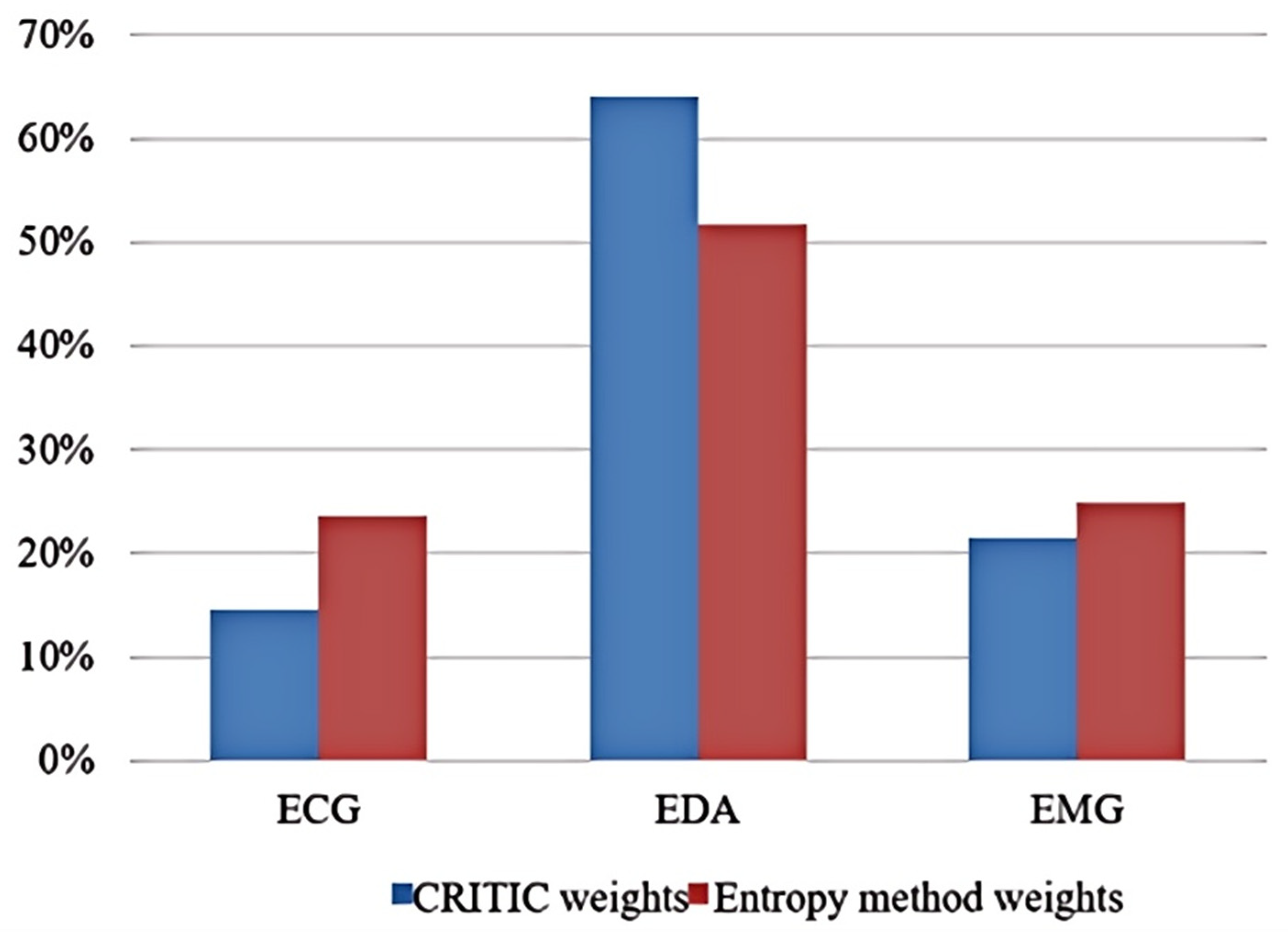
The weights of MMS_ECG, MMS_EDA, and MMS_EMG were calculated using the entropy method, and their weight values are 0.235, 0.517, and 0.248, respectively. The weights among the items are about 0.333, which is relatively uniform.

5.3. Analysis of Evaluation Parameters Based on Gray Relational Method

Gray system theory is a theory used to study and deal with complex systems. The theory begins by acknowledging the incompleteness of information and processes information mathematically at a certain level of the system, rather than analyzing it based on the specific laws within the system. This approach allows for a higher-level understanding of the trend of change and interrelationships within the system. To evaluate the automotive simulation system, the gray correlation theory analysis method can be applied, assuming that the biopsychological evaluation index of the simulation system is incomplete. This method considers the evaluation index of the simulation system as a gray system, and the specific steps of the evaluation are as follows:

• Determine the evaluation indicators and collate the indicator values to obtain the matrix to be evaluated;
• Determine the reference series, the value of which consists of the best value among the indicators;
• Dimensionless processing of evaluation index values.

Calculate the correlation coefficient and index score of the comparison sequence and the reference sequence as shown in Formula (27):

$${\xi }_i\left(j\right)={\displaystyle \frac{{max}_i{min}_j\left|X_0\left(j\right)-X_i\left(j\right)\right|+\rho {max}_i{max}_j\left|X_0\left(j\right)-X_i\left(j\right)\right|}{\left|X_0\left(j\right)-X_i\left(j\right)\right|+\rho {max}_i{max}_j\left|X_0\left(j\right)-X_i\left(j\right)\right|}}$$

(27)

Calculate the gray correlation (total indicator score). The indicator scores are weighted with the indicator weights to obtain the indicator scores corresponding to the total indicator layer as shown in Formula (28):

$${\gamma }_h=\sum s_j{w}_j\left|h=1,2,3,4\right.$$

(28)

According to the calculation method, the correlation results were obtained by substituting the model data as shown in

Table 5. Correlation result.

Appraisal Items	Correlation Degree	Rank
MMS_ECG	0.669	3
MMS_EDA	0.870	1
MMS_EMG	0.737	2

.

Based on the table above, gray correlation analysis was conducted on three evaluation items (MMS_ECG, MMS_EDA, and MMS_EMG) and the corresponding biopsychological data from the standard field experiment. As no “reference value” was provided, the maximum value of each evaluation item was used as the default “reference value” for the analysis. The discrimination coefficient used in the gray correlation analysis was 0.5, and the final correlation value ranged from 0 to 1. A higher correlation value indicates a stronger correlation with the “reference value” (parent series), which in turn indicates a higher evaluation. The table above indicates that MMS_EDA received the highest overall rating (correlation: 0.870) among the three evaluations, followed by MMS_EMG (correlation: 0.737). This finding is consistent with the overall pattern of weights derived from CRITIC and the entropy value method, which confirms the reliability of the above assignment from another perspective.

After obtaining the weights of the evaluation indicators of the simulator through the entropy method and CRITIC analysis, a comprehensive comparison was conducted, and the comparison results are shown in Figure 13.

According to the weighting analysis of evaluation indicators by the entropy value method and CRITIC analysis method, the overall weight allocation ratio trend is consistent, regardless of the variability of EDA, ECG, EMG, and the conflict between evaluation indicators from the standard experimental driving biopsychological indicators of the simulator, or the amount of effective information of EDA, ECG, and EMG, is used to assign weights. To effectively improve the respective advantages of the entropy method and CRITIC analysis method, the article selected a combination of the two methods to determine the weights of the simulator evaluation indicators, and after calculating the indicator weights $w_i$ for the entropy method and wk for the CRITIC method, the integrated weights were calculated as shown in Formula (29):

$${\xi }_t={\displaystyle \frac{w_{it}{w}_{kt}}{{\displaystyle {\sum }_{t=1}^n}{w}_{it}{w}_{kt}}}$$

(29)

The comprehensive weight for obtaining the indicators of the car simulator is finally determined. According to specific calculations, the comprehensive indicator weights of ECG, EDA, and EMG for test driving are selected by using the error evaluation indicators and two parameter property values obtained from the model operation to characterize the data situation, and set as the lowest level of the evaluation hierarchy. The weights of ECG, EDA, and EMG are assigned values of 0.5, 0.5, and 0.5, respectively. Based on the weight allocation, the simulator’s comprehensive evaluation value is set as shown in Formula (30) for the car simulator comprehensive evaluation model based on the driver’s psychological state.

$$\xi =\left({\xi }_1{w}_1+{\xi }_2{w}_{2i}\right)\times 100$$

(30)

The prediction error index of the test simulator model is summarized in

Table 6. Model prediction error evaluation index summary.

Item	${\mathit{R}}^2$	Rank Correlation	w	ξ
EMG	71.22%	77.92%	80.08%	12.71%
ECG	97.39%	90.54%	73.57%	8.16%
EDA	96.62%	97.75%	64.90%	79.12%

. According to the parameter values in the above table, the comprehensive evaluation index of the test simulator is obtained as 94.04, which indicates that the test simulator reaches an intermediate to advanced effective level and can meet the demand of more complex simulation applications in the traffic field with better robustness and applicability. It also indicates that the designed simulator standard scenario can effectively reflect both the actual human raw mental performance in the simulator experiment and the real traffic characteristics of the driver in the car driving simulation experiment in a simple and efficient way.

6. Conclusions

The paper utilizes the characteristics of deep learning models such as good nonlinear fitting and deep feature mining ability to solve modeling problems such as simulator parameters with nonlinearity and uncertainty. Considering the heterogeneity of human factor parameters such as ECG, EMG and EDA, the standard experimental data statistical interval is designed to be 0.2 s according to human reaction time to ensure that the model can identify human factor parameters in a timely and efficient manner. At the same time, to avoid interference such as driving fatigue caused by the complexity of the scene, the experimental duration is set to about 10 min and the experimental mileage is about 10 km.

An integrated machine learning method based on the LSTM model is constructed to transform the experimentally collected simulator high-dimensional multi-attribute data into a two-dimensional matrix and then input it into the integrated machine learning model. The integrated machine learning model is based on Bayesian optimization for hyperparameter tuning, and reflects the experimental performance of the simulator with the driver’s biopsychological indicators in the simulator experiment by matching the driver’s causal characteristics. The integrated machine learning method based on the LSTM model improves the deficiency of single-parameter prediction of the integrated machine learning method and makes it applicable to high-dimensional multi-attribute simulator data evaluation.

The specific prediction results of the model are as follows: Based on the entropy value method and CRITIC analysis of the evaluation indicators for weighting analysis, the overall trend of the proportion of weight distribution is consistent, whether it is from the variability of EDA, EMG, ECG and the conflict between the evaluation indicators in the simulator standard experimental driving biopsychological indicators, or the use of the amount of effective information to assign weights. Combining the weights of both indicators, the EDA, EMG, and ECG weights are 79.12%, 12.71%, and 8.16%, respectively. This yields a comprehensive evaluation indicator of 94.04 for the test simulator, indicating that it achieves a medium to high level of validity and can meet the needs of more complex simulation applications in the traffic field. This shows that the test simulator can meet the requirements of complex simulation applications in the traffic field, and it shows that the standard scene designed by the paper can effectively reflect and evaluate the actual biopsychological performance of people in the experiment, and can also simply and effectively reflect the real traffic characteristics of drivers, and the model has good robustness and applicability.

This paper has several limitations, and future research can be carried out in the following aspects: First, this study mainly focuses on the biopsychological characteristics of experienced drivers. Future research could increase the sample size to examine the differences in characteristics among drivers of different genders, ages, and personality types. Second, the driver characteristic parameter system can be further expanded. In the future, visual perception, EEG signals, vehicle speed parameters, and other sensory parameter data could be integrated to build a comprehensive evaluation model and improve the overall performance of the model. Third, the results of this paper are mainly based on controlled risk conflict scenarios in driving simulators, reflecting the simulator’s ability to reproduce drivers’ behavioral and physiological–psychological responses in such scenarios. Therefore, the evaluation results in this paper should be understood as the internal validity of the simulator under controlled experimental conditions and cannot be directly equated with the external validity under real-road driving conditions. Future research still needs to combine real-road experiments, closed-field experiments, or natural driving data to further compare and verify the simulator experiment results. Finally, this paper has not yet conducted a direct comparison with real-road or natural driving data. Future research could use closed-field tests, real-road driving tests, or natural driving data to compare simulator data with real driving data in terms of speed, braking behavior, reaction time, vehicle trajectory, EDA, ECG, and EMG, in order to further verify the external validity of the evaluation framework proposed in this paper.

References

1. Chen, L. Research on the Validation of Vehicle Driving Simulator Based on Driver’s Traffic Characteristics. Ph.D. Thesis, Kunming University of Science and Technology, Kunming, China, 2021. (In Chinese) [Google Scholar]
2. Kang, M.-W.; Momtaz, S.U. Assessment of driver compliance on roadside safety signs with auditory warning sounds generated from pavement surface–a driving simulator study. J. Traffic Transp. Eng. 2018, 5, 1–13. [Google Scholar] [CrossRef] [Scilit]
3. Wynne, R.A.; Beanland, V.; Salmon, P.M. Systematic review of driving simulator validation studies. Saf. Sci. 2019, 117, 138–151. [Google Scholar] [CrossRef] [Scilit]
4. Wang, X.L.; Li, L.; Zhang, W.H. Analysis of Driving Simulator Realism Based on Platform Institution Size Parameters. J. Mach. Des. 2009, 26, 53–57. Available online: https://kns.cnki.net/kcms/detail/detail.aspx?dbcode=CJFD&dbname=CJFD2009&filename=JXSJ200905016 (accessed on 16 June 2026). (In Chinese)
5. Groeger, J.A.; Murphy, G. Driver performance under simulated and actual driving conditions: Validity and orthogonality. Accid. Anal. Prev. 2020, 143, 105593. [Google Scholar] [CrossRef] [Scilit] [PubMed]
6. Hussain, Q.; Alhajyaseen, W.K.M.; Pirdavani, A.; Reinolsmann, N.; Brijs, K.; Brijs, T. Speed perception and actual speed in a driving simulator and real-world: A validation study. Transp. Res. 2019, 62, 637–650. [Google Scholar] [CrossRef] [Scilit]
7. Wang, J.Z.; Jiang, S.; Wang, S.K.; Shen, W. Research of Somatosensory Simulation Algorithm Based on Six-Degree-of-Freedom Platform. Trans. Beijing Inst. Technol. 2021, 41, 728–733. (In Chinese) [Google Scholar]
8. Zoeller, I.; Abendroth, B.; Bruder, R. Driver behaviour validity in driving simulators—Analysis of the moment of initiation of braking at urban intersections. Transp. Res. Part F Traffic Psychol. Behav. 2017, 61, 120–130. [Google Scholar] [CrossRef] [Scilit]
9. Zhang, Y.N.; Guo, Z.Y.; Li, Z.J. Driving Simulator Validation Study Under Car-following Condition. J. Tongji Univ. (Nat. Sci.) 2020, 48, 847–853. (In Chinese) [Google Scholar] [CrossRef]
10. Pawar, N.M.; Velaga, N.R.; Sharmila, R.B. Exploring behavioral validity of driving simulator under time pressure driving conditions of professional drivers. Transp. Res. Part F. Traffic Psychol. Behav. 2022, 89, 29–52. [Google Scholar] [CrossRef] [Scilit]
11. Llopis-Castelló, D.; Camacho-Torregrosa, F.J.; Marín-Morales, J.; Pérez-Zuriaga, A.M.; García, A.; Dols, J.F. Validation of a Low-Cost Driving Simulator Based on Continuous Speed Profiles. Transp. Res. Rec. 2016, 2602, 104–114. [Google Scholar] [CrossRef] [Scilit] [PubMed]
12. Cao, C.; Wang, J.; Luo, Y. Driving simulator validation for research on driving behavior at entrance of urban underground road. In Proceedings of the 2015 International Conference on Transportation Information & Safety, Wuhan, China, 25–28 June 2015. [Google Scholar]
13. Martin-Castresana, S.; Alvarez, D.; Andrade-Cataño, F.; Castro, M. Effect of Road Markings on Speed through Curves on Rural Roads: A Driving Simulator Study in Spain. Infrastructures 2025, 10, 94. [Google Scholar] [CrossRef] [Scilit]
14. Talsma, T.M.W.; Hassanain, O.; Happee, R.; de Winkel, K.N. Validation of a moving base driving simulator for motion sickness research. Appl. Ergon. 2023, 106, 103897. [Google Scholar] [CrossRef] [Scilit] [PubMed]
15. Larue, G.S.; Wullems, C.; Sheldrake, M.; Rakotonirainy, A. Validation of a Driving Simulator Study on Driver Behavior at Passive Rail Level Crossings. Hum. Factors 2018, 60, 743–754. [Google Scholar] [CrossRef] [Scilit] [PubMed]
16. Zhao, Z.G.; Feng, J.X.; Zhou, L.J.; Wang, K.; Hu, H.; Yhang, H. K-means Clustering and Recognition of Driver’s Collison Avoidance Steering Behavior. Automot. Eng. 2020, 42, 52–58. (In Chinese) [Google Scholar] [CrossRef]
17. Nacpil, E.J.; Kaizuka, T.; Nakano, K. Driving Simulator Validation of Surface Electromyography Controlled Driving Assistance for Bilateral Transhumeral Amputees. Adv. Intell. Syst. Comput. 2020, 958, 166–175. [Google Scholar]
18. Nacpil, E.J.; Nakano, K. Driving Simulator Validation of Machine Learning Classification for a Surface Electromyography-Based Steering Assistance Interface. In Proceedings of the Advances in Intelligent Systems and Computing, Virtual, 25–29 July 2021; pp. 143–149. [Google Scholar]
19. Healey, J.A.; Picard, R.W. Detecting Stress during Real-World Driving Tasks Using Physiological Sensors. IEEE Trans. Intell. Transp. Syst. 2005, 6, 156–166. [Google Scholar] [CrossRef] [Scilit]
20. Kierzkowski, A.; Wolniewicz, Ł.; Danilevičius, A.; Mardeusz, E.; Kin, M.; Bakinowski, Ł.; Barabasz, D.; Wielkopolan, P. The Concept of a Universal Tram Driver Console with Interchangeable Panels for a Polish Tram Simulator. Infrastructures 2024, 9, 41. [Google Scholar] [CrossRef] [Scilit]
21. Paliotto, A.; Meocci, M. Development of a Network-Level Road Safety Assessment Procedure Based on Human Factors Principles. Infrastructures 2024, 9, 35. [Google Scholar] [CrossRef] [Scilit]
22. Ghulam, H.B.; Durga, M.; Ming, L.; Vallati, M. Younger driver’s evaluation of vehicle mounted attenuator markings in work zones using a driving simulator. Transp. Lett. Int. J. Transp. Res. 2010, 2, 187–198. [Google Scholar] [CrossRef] [Scilit]
23. Bella, F. Driving Simulator for Speed Research on Two-Lane Rural Roads. Accid. Anal. Prev. 2008, 40, 1078–1087. [Google Scholar] [CrossRef] [Scilit] [PubMed]
24. Liu, Z.; Yang, Q.; Wang, A.; Gu, X. Vehicle Driving Safety of Underground Interchanges Using a Driving Simulator and Data Mining Analysis. Infrastructures 2024, 9, 28. [Google Scholar] [CrossRef] [Scilit]
25. Bosurgi, G.; Di Perna, M.; Pellegrino, O.; Sollazzo, G.; Ruggeri, A. Drivers’ Steering Behavior in Curve by Means of New Indicators. Infrastructures 2024, 9, 43. [Google Scholar] [CrossRef] [Scilit]
26. Li, S.T.; Yang, H.; Cheng, R.J.; Ge, H. Hybrid deep learning models for short-term demand forecasting of online car-hailing considering multiple factors. Transp. Lett. 2023, 16, 218–233. [Google Scholar] [CrossRef] [Scilit]
Figure 1. The technical route of this paper.
Infrastructures 11 00220 g001
Figure 2. Driving simulator for testing: true car cab (a), self-built cockpit (b).
Infrastructures 11 00220 g002
Figure 3. Diagram of driver wearing wireless EDA, ECG, and EMG sensors. Note: The driver’s wireless sensor kit has three ECG leads on the chest in red, blue, and black; the EMG on the arm holding the steering wheel only uses red and black, no blue needed.
Infrastructures 11 00220 g003
Figure 4. Experimental dynamic and static scene diagram: (a) no signal and no occlusion conflict port, (b) no signal and occlusion conflict port, (c) no signal and low flow conflict port, (d) no signal and heavy flow conflict port, (e) dynamic virtual scene.
Infrastructures 11 00220 g004
Figure 5. The schematic flow of the evaluation model.
Infrastructures 11 00220 g005
Figure 6. Bayesian hyperparameter optimization algorithm.
Infrastructures 11 00220 g006
Figure 7. Comparation of R2: (a) EMG, (b) ECG, (c) EDA.
Infrastructures 11 00220 g007
Figure 8. Error comparison diagram: (a) EMG, (b) ECG, (c) EDA.
Infrastructures 11 00220 g008
Figure 9. Comparation of rank correlation: (a) EMG, (b) ECG, (c) EDA.
Infrastructures 11 00220 g009
Figure 10. Comparison of mean deviation: (a) EMG, (b) ECG, (c) EDA.
Infrastructures 11 00220 g010
Figure 11. Optimization effect comparison: (a) EMG (b) ECG (c) EDA.
Infrastructures 11 00220 g011
Figure 12. Two- to 10-fold cross-validation R2.
Infrastructures 11 00220 g012
Figure 13. CRITIC–entropy method weight diagram.
Infrastructures 11 00220 g013