Article

Evaluation of Connected Vehicle Pavement Roughness Data for Statewide Needs Assessment

Lyles School of Civil and Construction Engineering, Purdue University, West Lafayette, IN 47907, USA
*
Author to whom correspondence should be addressed.
Infrastructures 2025, 10(9), 248; https://doi.org/10.3390/infrastructures10090248
Submission received: 5 August 2025 / Revised: 5 September 2025 / Accepted: 15 September 2025 / Published: 18 September 2025
(This article belongs to the Section Smart Infrastructures)

Abstract

Many agencies use pavement condition assessments such as the Pavement Surface Evaluation and Rating (PASER) and Pavement Condition Index (PCI) to develop localized pavement management programs. However, both techniques involve some subjectivity and inconsistent measurement practices, making it difficult to scale uniformly across all 86 thousand miles of local agency roadway in Indiana’s 92 counties. International Roughness Index (IRI) data is one emerging data source that could address this need. This paper evaluates the feasibility of using Connected Vehicle-estimated IRI (IRICVe) data for long-term statewide pavement monitoring on local roads. The analysis is based on approximately 4.1 billion daily IRICVe records collected over a multi-year study period from connected vehicles operating throughout the state. A modular data processing workflow was developed to clean and process these records and is presented in detail in the paper. The study includes network-level condition comparisons, insights on spatiotemporal trends, and localized segment-level condition monitoring. In 2024, approximately 53% of paved local roads in Indiana had at least one IRICVe observation per year. Coverage varied widely by county: for example, 79% of roads in urban Hamilton County had coverage, but only 14% had coverage in rural Martin County. The findings in this study demonstrate the potential of IRICVe to support local agency pavement asset management by providing cost-effective data-driven insights in near real-time.

1. Introduction

Pavement condition data is foundational to effective roadway maintenance planning and investment prioritization. Traditionally, condition monitoring has relied on visual inspection methods such as the Pavement Condition Index (PCI) or Pavement Surface Evaluation and Rating (PASER) [1,2]. While these metrics remain widely used and focus on the pavement degradation and failure characteristics, they are also quite subjective and often do not reflect the ride quality that the vehicle experiences. In contrast, the International Roughness Index (IRI) provides a quantitative value that is well correlated with perceived ride quality. IRI measurements taken with conventional methods are still costly and often limited to higher traffic roadways, however. In Indiana, IRI is surveyed annually for all state-maintained highways [3]. In recent years, fleets of connected vehicles (CVs) have enabled the collection of highly granular, crowdsourced IRI estimates at scale. This represents a transformative shift for transportation agencies, particularly for those with limited resources.
Despite this promise, significant barriers remain to the widespread adoption of CV-estimated IRI (IRICVe) data. Agencies face challenges related to data ingestion, storage, quality control, integration, and analysis. The large volume of billions of records a year also poses a challenge. Many agencies are not equipped to handle data of this scale, and the lack of detailed, standardized data pipeline documentation has hindered efforts to integrate IRICVe into traditional asset management practices [4].

1.1. Paper Objective

The objective of this paper is to present a modular and transparent workflow for processing IRICVe at a statewide scale, with a focus on Indiana’s paved local roadway network. The methodology includes route deduplication, segmentation, buffering, and scalable techniques to join multiple data sources such as IRICVe and surface type. The approach is applied to over 78,000 miles of paved roadways managed by local agencies (state-managed roads are excluded). In addition to detailing the data processing pipeline, the paper also evaluates spatial and temporal coverage of the CV data, compares roughness distributions across counties and roadway classes, and illustrates practical use cases for condition screening and post-maintenance verification. The methodology and findings provide a blueprint for local and state transportation agencies seeking to integrate CV data into their asset management systems.

1.2. Literature Review

Established pavement condition metrics such as PCI and PASER have been widely adopted for local-scale monitoring. While traditionally based on manual surveys, recent studies have explored using computer vision and machine learning for limited automation of data collection. However, these automated approaches remain difficult to deploy at scale due to challenges such as class imbalance and the lack of large-scale, annotated datasets for validation and training [5,6].
The PCI is a metric ranging from 0 (failed) to 100 (excellent) based on visual inspection of the pavement surface distresses. According to the ASTM D6433 document, which outlines the standard practice for PCI evaluation, this inspection should be performed by manually walking the length of the road segment, which it states can be dangerous in traffic [7]. Additionally, PCI assessments are based on a sample of pavement units rather than a full census, and the sampling method can vary between agencies, affecting data consistency. PASER similarly relies on visual inspection, although it is often measured from a moving vehicle and ranges from 0 to 10 [8]. Both systems use subjective criteria such as “slight”, “moderate”, or “severe” distress severity, which introduces substantial inter-rater variability. These limitations make it difficult to scale up to consistent and objective statewide condition monitoring.
In contrast, the IRI offers a more objective, ride quality-based metric, often in units of m/km or in/mi. IRI is typically measured with high-speed inertial profilers [9], although recent studies have used new methods like image processing [10] and Light Detection and Ranging (LiDAR) [11]. While IRI does capture the impact of surface distresses on ride quality, it accounts for neither the cause of this displacement nor distresses like rutting or longitudinal cracking that do not vertically displace the vehicle. Nonetheless, it is still useful in combination with other metrics to quantify roughness for condition screening and investment prioritization.
More recently, IRI estimates have been derived using crowdsourced data from CVs, leveraging Original Equipment Manufacturer (OEM) sensors to provide dense, near real-time coverage at network scale. This method offers a production-ready, cost-effective alternative to traditional data collection. Additionally, aggregation over multiple crowdsourced measurements provides a more holistic and robust IRI value. Several vendors already deliver IRICVe, and validation studies have demonstrated strong correlations with profiler-based IRI data. By aligning data collected from both sources to the same linear reference segments, these studies report R2 coefficients ranging from 0.70 to 0.79 [12,13]. Despite these positives, there are some limitations of IRICVe data that are not present in manually collected IRI data. The IRICVe dataset used in this study was collected solely from passenger vehicles [14], and omits trucks, buses, and motorcycles. Furthermore, Llopis-Castelló et al. reported that IRICVe slightly underestimates the IRI found by profiler survey for distressed road segments, suggesting that this discrepancy could be due to drivers typically avoiding wheel paths with roadway distresses [15]. Quantitatively, a recent study reports 230 km of field tests with an overall RMSE ≈ 0.37 m/km when using vertical vibrations detected by onboard Inertial Measurement Unit (IMU) sensors, which are within 1–10% of the reference values [16].
Most prior work with this data has focused on arterial and interstate routes [17], with limited evaluation of its use for large-scale condition monitoring of local road networks. In addition, few studies have analyzed spatial coverage, which is an important metric for agencies to gauge expected data availability after integration.
Importantly, the large volume and high granularity of IRICVe introduce nontrivial challenges in ingestion, storage, cleaning, and analysis. Several billion IRICVe records are ingested every year in the state of Indiana alone. This scale far exceeds that of typical transportation datasets and requires robust data engineering workflows. Mussah et al. emphasized the importance of careful workflow planning and noted that terabyte-scale CV datasets can have processing times reduced by as much as 70× with properly applied GPU-acceleration [18]. Geospatial big data also demands specialized storage, indexing, and quality control strategies to ensure consistency [19]. These challenges pose a significant barrier to widespread adoption by agencies, which may not have the trained workforce to properly handle the data. Despite increasing interest in IRICVe and existing documentation by the Transportation Research Board (TRB) on general data system development [20], current literature provides little guidance for state and local agencies on how to specifically integrate CV-based condition monitoring datasets into their asset management workflows.
While existing studies validate the accuracy of IRICVe [12,13], they seldom address the practical issues of agency-level adoption, including the creation of robust data processing pipelines, integration with cloud computing infrastructure, and optimization for big data. This paper addresses these gaps by presenting a scalable, transparent data workflow tailored to agency needs and evaluates its use for statewide condition monitoring with an emphasis on spatial coverage and applicability to rural and local roads.

2. Methods

This section describes the data sources used for the study and outlines a scalable data processing workflow for CV-based condition monitoring.

2.1. Data Sources

The following subsections describe the study location and data sources including the US Roads Dataset, IRICVe data, and surface type data.

2.1.1. Study Location

This study was conducted in the state of Indiana, including the local networks for all 92 counties (Figure 1). According to the 2024 Local Road and Bridge Report, local agencies are responsible for the maintenance of 85,954 centerline miles of roadway, which accounts for approximately 89% of all Indiana centerline miles [21].

2.1.2. US Roads Dataset

The US Roads Dataset was used as an independent route source, which is available publicly free of charge on the BigQuery Marketplace [22]. The data are derived from the US Census Bureau’s Topologically Integrated Geographic Encoding and Referencing (TIGER) database and contain comprehensive route lines for all US states and territories. Notably, the data include functional classification classes that were used for determining local and state-managed routes.

2.1.3. IRICVe Data

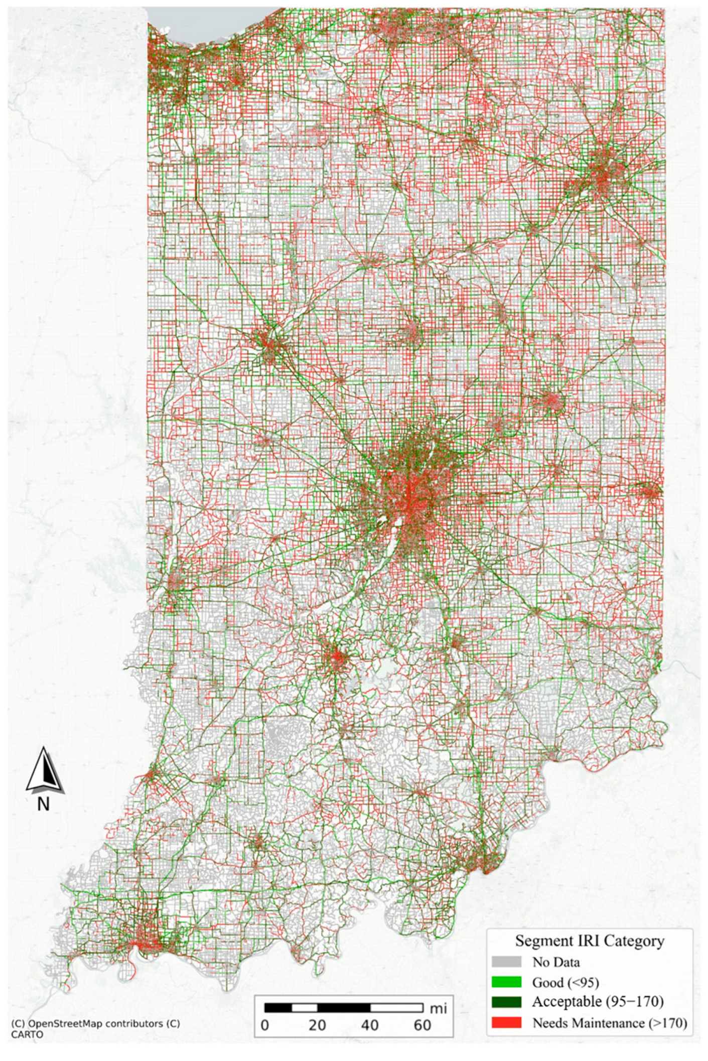
This study utilizes IRICVe data collected by onboard sensors from a fleet of connected vehicles, with anonymized data obtained through a commercial third-party vendor. A Kalman filter is used to fuse data from multiple sensors, such as the GPS and IMU, which are used to measure vehicle speed and chassis vibration. This multi-sensor fusion approach efficiently estimates the road’s longitudinal profile, which is then used to calculate its IRI value [16]. The data are provided as short road segments ranging from 50 to 85 feet in length, updated on a daily basis. Each segment’s IRICVe estimate represents a 60-day moving average over the CV measurements, and each measurement is converted from experienced roughness to the standard IRI scale with units of inches per mile (in/mi), representing the vertical displacement in inches over the longitudinal movement in miles along the roadway. To classify roughness, Federal Highway Administration (FHWA)-defined thresholds were used: segments were labeled as Good (<95 in/mi), Acceptable (95–170 in/mi), and Needs Maintenance (>170 in/mi) [23]. Figure 2 visualizes these data aggregated over the year of 2024 to aid in conveying the scale.

2.1.4. Surface Type Data

The study also uses an Indiana Department of Transportation (INDOT) pavement surface type shapefile provided by the Indiana Geographic Information Office through the public IndianaMap GIS portal [24]. This shapefile includes roadway centerlines with attributes including the surface material, such as asphalt, concrete, or gravel. Each feature includes a surface type designation along with route and location metadata, allowing for integration with other datasets through spatial joins, although data are only available for one direction of bi-directional roadways.

2.2. Data Infrastructure

CV data are typically collected by OEM sensors embedded in vehicles. Initial pre-processing for driver privacy protection may be performed before the data are sent to a third-party vendor. These vendors serve as intermediaries, performing additional quality assurance and processing to make the data more accessible and to meet client requirements. Clients receive the data by either periodic data dump files or by requesting it with secure Application Programming Interfaces (APIs). Although data dumps are simple to implement, APIs offer real-time, flexible access, with more complex infrastructure. A consistent file-naming convention, data table schema, and programmatic quality verification are important for keeping the data clean and accurate.
Once received and verified, the data are inserted into a centralized database, which may be hosted on local servers or, increasingly, on cloud-based platforms, due to their performance and accessibility. For this study, a cloud service was used to store, manage, and process over 4 billion records of IRICVe data across the entire state of Indiana. The platform enabled efficient handling of terabyte-scale datasets, taking only a few minutes to execute the following data processing workflow for years of high-granularity statewide CV data when carefully optimized. The optimizations were made to both reduce time taken and bytes scanned, the latter of which is typically used to calculate the query cost; The cost of querying was approximately $6.25 per terabyte scanned [25].
For intermediate analysis, transformation, and visualization, a combination of cloud-based and local tools was employed. Web-based tools were used for geospatial inspection of datasets directly from the cloud [26]. For more granular analysis and customized visualization, Python 3.12 and R 4.5 were used locally. Both environments offer mature libraries such as pandas-gbq and bigrquery for database access, and matplotlib, plotnine, and ggplot2 for visualization. While R is widely adopted by transportation agencies for data analysis workflows, Python offers broader applicability across data engineering and machine learning domains.

2.3. Route Network Preparation

2.3.1. Route Deduplication

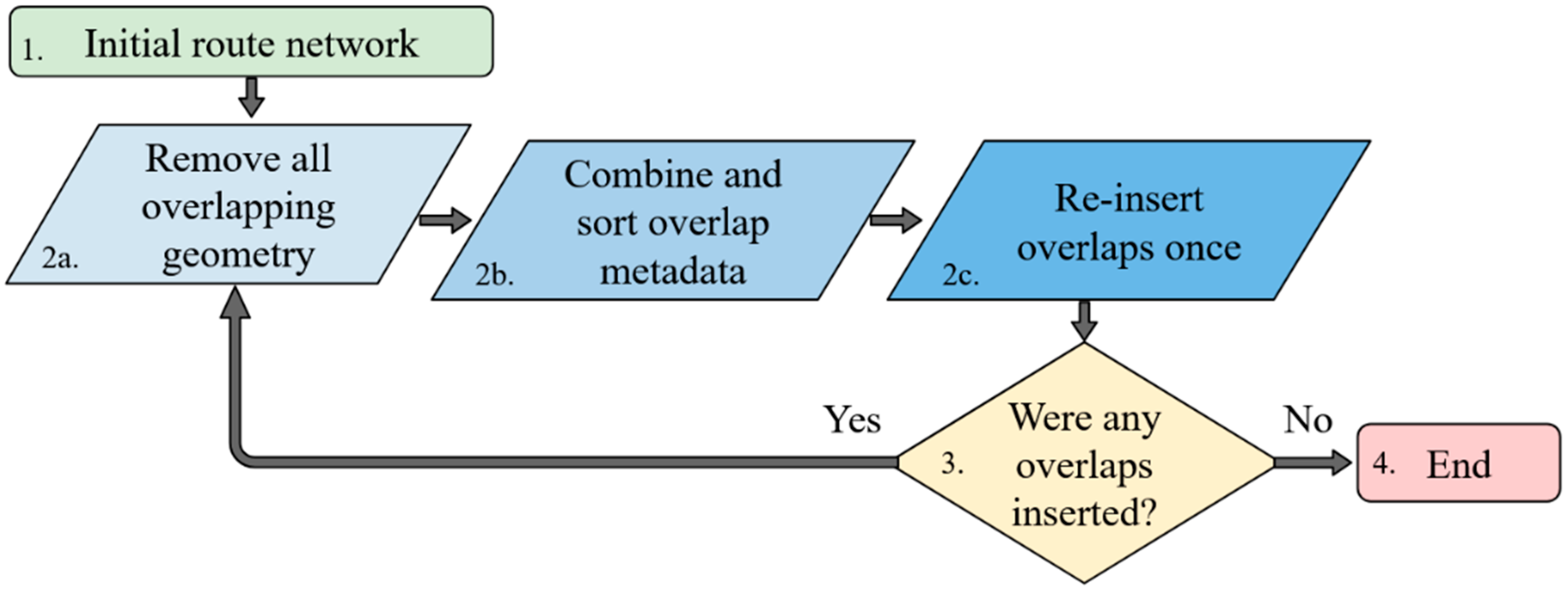
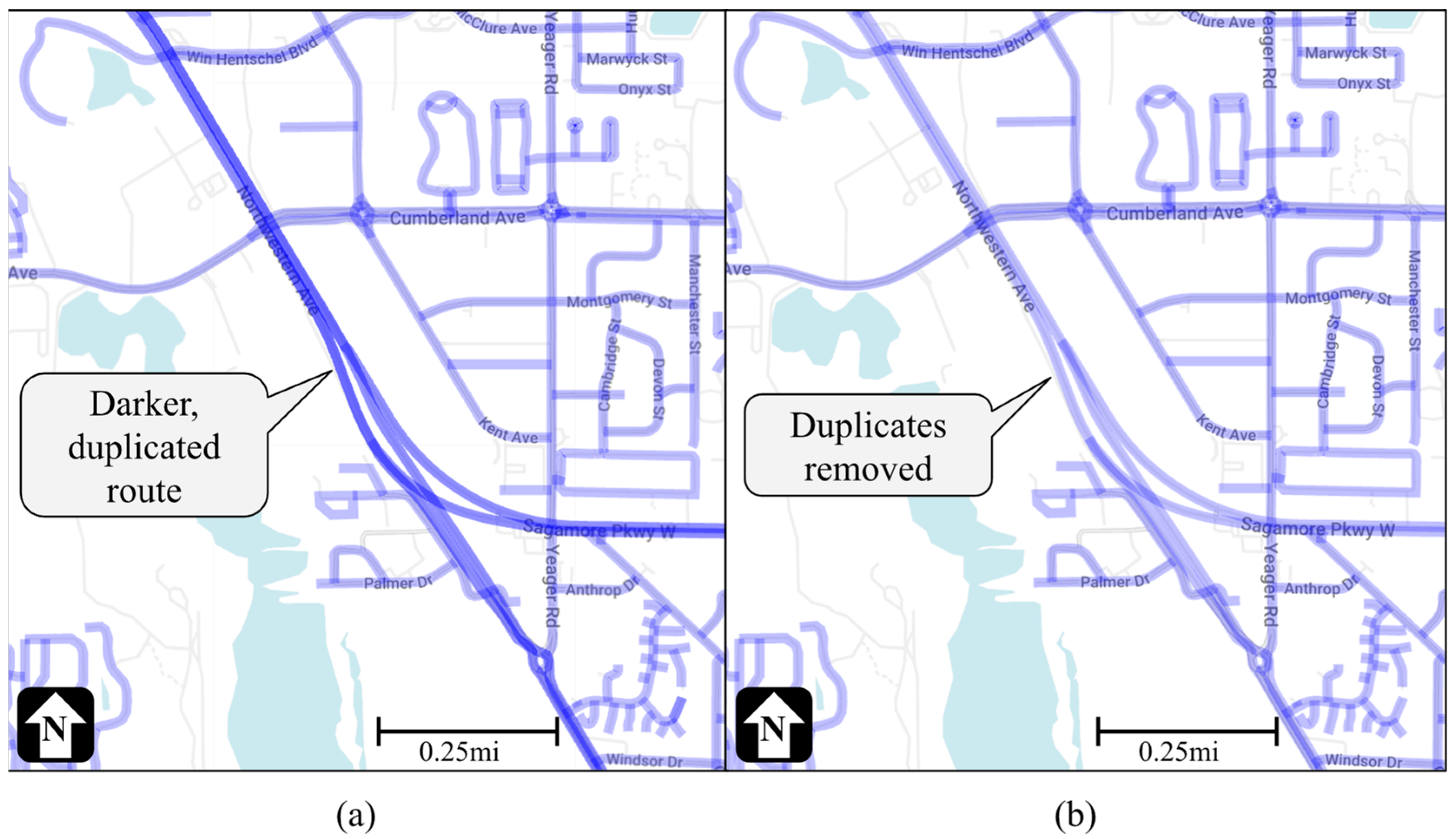
The US Roads dataset contains substantial overlapping geometry, often resulting from historical renaming or route changes. To address this, deduplication was implemented as the first step in the data processing pipeline. A simple yet effective algorithm was developed (Figure 3) to iteratively merge overlapping route geometries until no overlaps remain. To avoid combining intersections or consecutive segments, only overlaps longer than 5 m (16.4 feet) were considered. Figure 4 illustrates the effect of deduplication, showing how multiple overlapping geometries were consolidated into a single route. Since approximately 30% of the route data is duplicated, this step is essential to prevent oversampling and to ensure accurate analysis when using the US Roads dataset.

2.3.2. Route Preprocessing

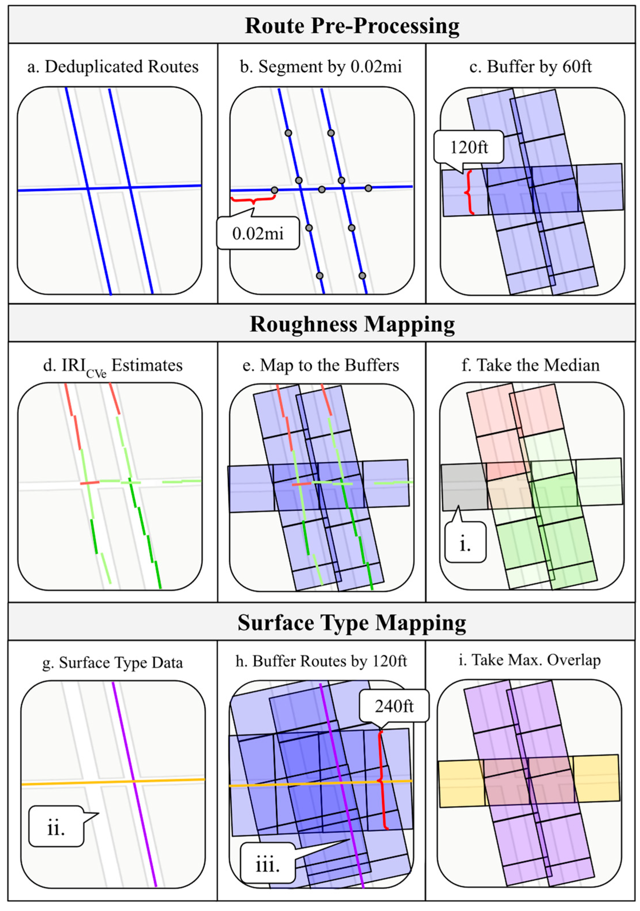
Following deduplication, metadata such as the county and district were sourced from publicly available shapefiles on IndianaMap [27,28] and joined with the existing route segments by choosing the county or district with the most spatial overlap. This greatly simplifies any county- and district-level aggregation and analysis downstream. Subsequently, as shown in Figure 5, these routes were segmented (step b.) and buffered (step c.).
Segmentation was performed at 0.02-mile intervals by generating substrings of the original line geometries, rather than sampling points and connecting them with straight lines. This approach preserves the original curvature of the road, meaning no data are missed on highly curved roads, which occur frequently in local networks. A 0.02-mile segment length was chosen for high spatial granularity in local road networks and for use with the ~75 ft (0.014 mi) IRI estimates. Agencies should adjust this length as necessary, given their data source granularity and application. As the segments are created, the segment ID is generated by appending the segment index to the base route ID that it is a part of. For each resulting segment, the undirected heading was calculated by using the segment’s start and end points to compute the azimuth bearing (the angle in radians clockwise from true north), converting it to degrees, and projecting it to a 0–180° range using modulus division. This transformation accounts for inconsistent line directionality in the base network (i.e., some segments may face opposite directions along the same corridor), while still allowing for directional filtering when joining with other data in subsequent steps. If the base route network has consistent directionality, then it is recommended to skip this step and to keep heading in the 0–360° range. Additionally, an algorithm can be developed to reverse route segments that are in the wrong direction so that every segment along a given route is facing the same way, although this was not needed for the use cases in this study.
A 60-foot buffer was applied to each segment using a flat endcap to avoid overlap between consecutive segments (step c). This buffer size was chosen to fully cover all lanes of all road classes and account for both variations in base map line work and GPS errors. Although somewhat subjective, this was found to be sufficient to account for the minor network and GPS errors but not erroneously include adjacent segments in dense urban areas.
To support long-term condition monitoring, it is recommended to assign an active and inactive date to each route segment. This allows for future updates to the base route network by inserting the new segments and marking the outdated ones as inactive. The processed route segments are stored in a permanent data table for efficient use in later processing steps and to ensure a consistent reference across queries.

2.3.3. Data Mapping

Two datasets were mapped to the route segments: IRICVe estimates and roadway surface type. The mapping process involves a combination of spatial joins and aggregations to assign one representative value per segment per time period. The process for one time period is illustrated in Figure 5, steps d–i.
Each IRICVe estimate was assigned to a single route segment by choosing the one with the lowest segment ID. This ensures a one-to-one mapping to prevent oversampling from estimates spanning multiple route segments. Assignments were also filtered on their headings by computing the difference in undirected heading between the estimate and route segment, and only keeping differences <10 and >170 for a tolerance of ±10°, accounting for heading wraparound. This will remove any data that intersects the segment at large angles, which are from other routes and should not be considered for aggregation.
Daily per-segment medians were first computed over all of the IRICVe estimates assigned to this segment in the previous step. Then, a second median is taken with these daily median values over a given time period. Although this study uses monthly and yearly time periods for aggregation, the time period can be adjusted as needed: shorter periods increase temporal precision and data volume, while longer periods have better data coverage and smaller storage volume at the cost of reduced temporal precision. Segments with no IRICVe data in a given period were assigned a value of −1 to clearly indicate that no data was found, as it falls outside of the possible IRI metric range. Critically, all route segments were retained in the output regardless of data coverage to facilitate downstream coverage analysis (Figure 5, callout i.). Therefore, every period will have an observation count equal to the number of route segments.
Surface type data were mapped using a 120-foot buffer, double that for the IRI estimates. This was performed because the surface type dataset only has data for one roadway direction (Figure 5, callout ii.), and the larger buffer increases the likelihood of capturing the relevant data from the other direction so that unknown surface types are minimized (Figure 5, callout iii.). Heading filtering was applied in the same way as the IRICVe data; however, paved surface types were prioritized over gravel and dirt surfaces. Among candidates with the same priority, the surface type with the maximum spatial overlap was selected.

3. Results

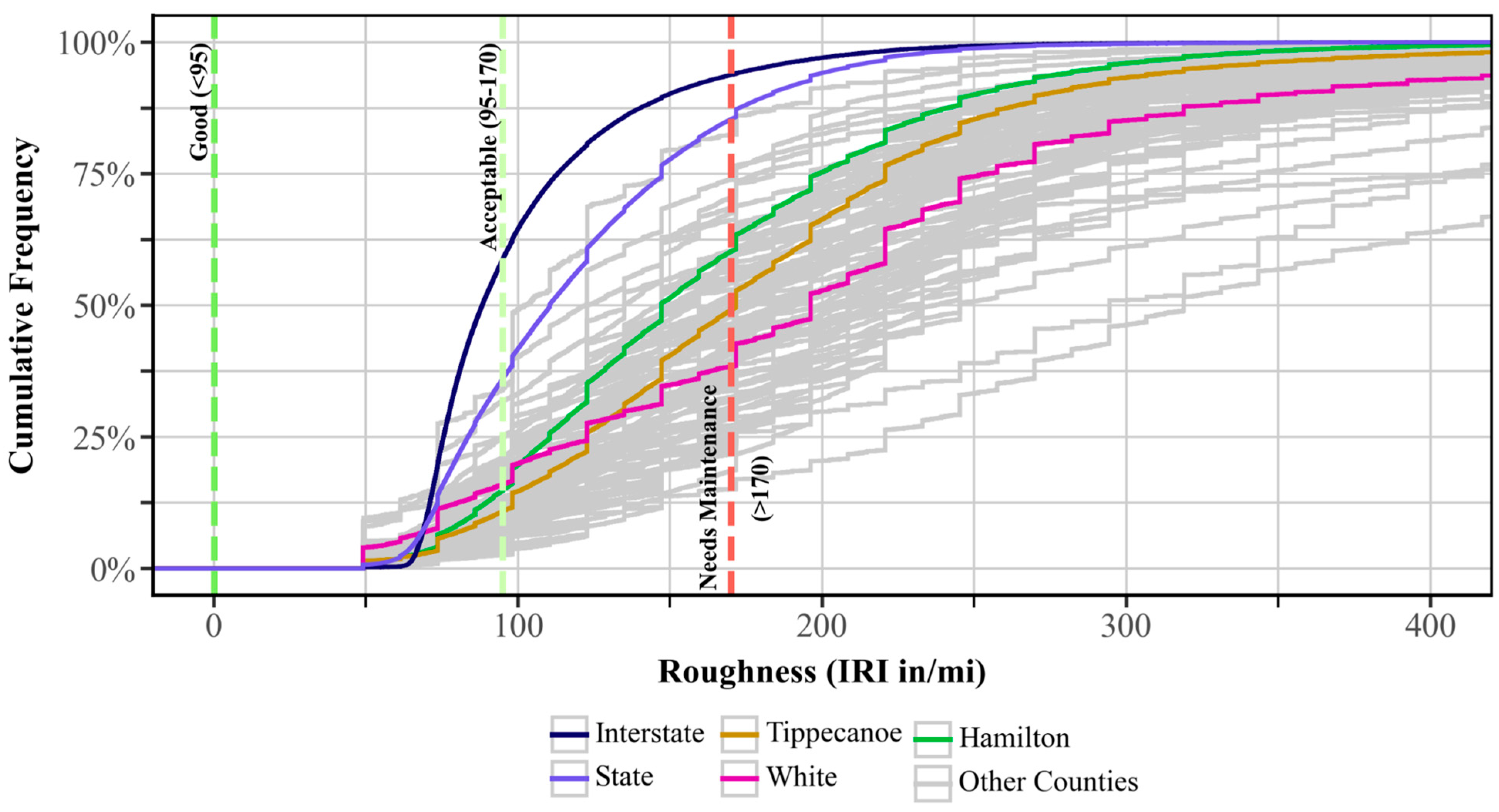
Figure 6 compares cumulative frequency distributions (CFDs) of segment-level IRICVe values across Indiana’s interstate, state, and local county road networks in 2024. Distributions are shown with no smoothing applied, and only segments with valid IRICVe values were included. The green, light green, and red vertical lines represent widely used FHWA IRI thresholds for “Good” (<95, green), “Acceptable” (95–170, light green), and “Needs Maintenance” (>170, red). Three counties, Hamilton, Tippecanoe, and White, were chosen as representative examples of urban, mid-sized, and rural infrastructure, respectively. Interstate routes show the lowest proportion of segments exceeding the “Needs Maintenance” IRI threshold, followed by state routes, with county routes generally being rougher. Among road segments with IRICVe data in the highlighted counties, Hamilton’s roads are smoothest, followed by Tippecanoe and White. This type of visualization enables rapid comparison of pavement condition distributions across multiple roadway networks and informs strategic planning and maintenance prioritization at a high level for transportation agencies.
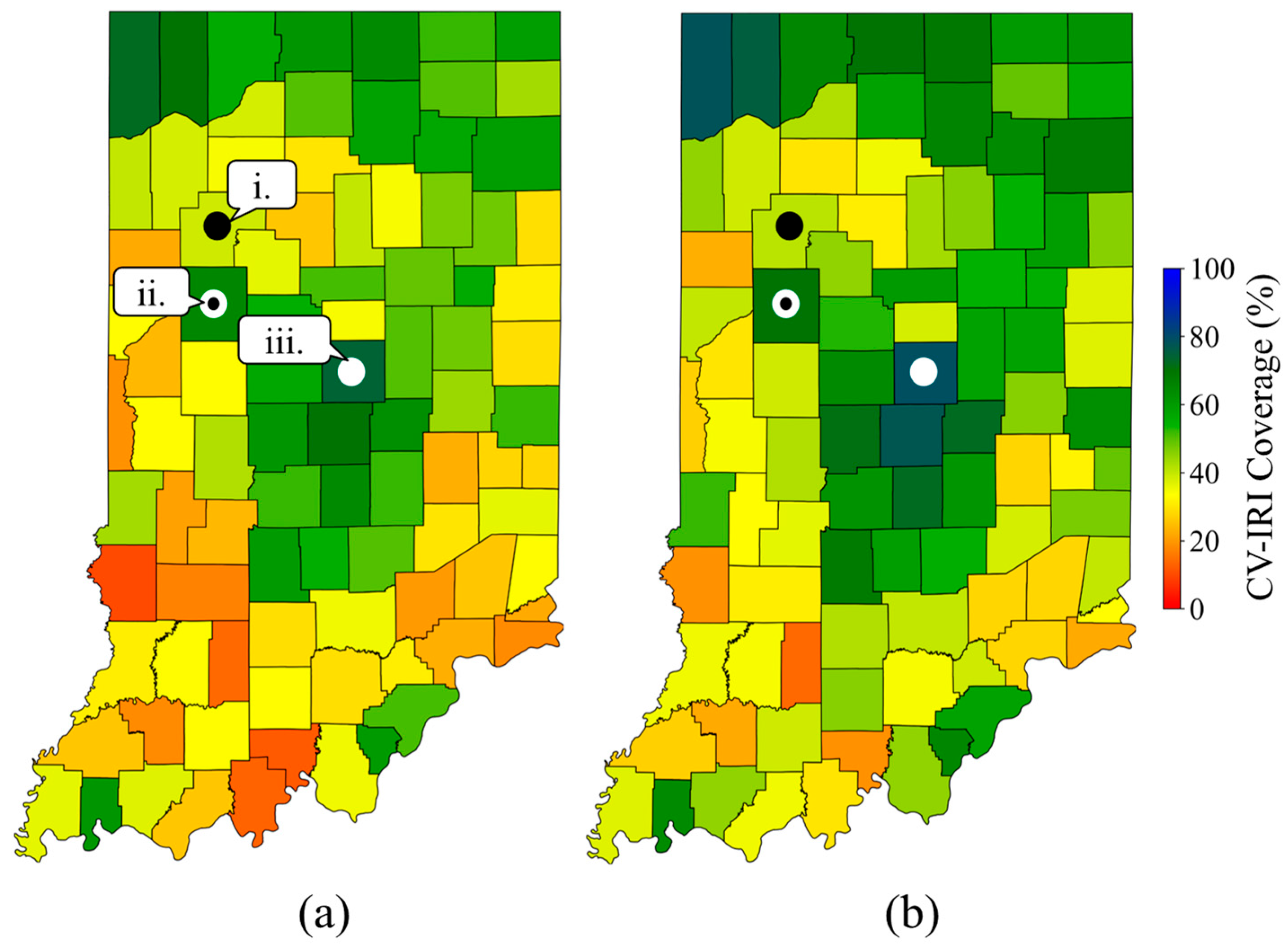
To assess statewide data availability for local paved roads, including spatial and temporal trends, two county-level coverage maps were created using IRICVe data from 2023 and 2024 (Figure 7a and Figure 7b, respectively). For each figure, a county’s data coverage is defined as the proportion of segments with at least one valid IRICVe observation that year. Callouts i., ii, and iii correspond to White, Tippecanoe, and Hamilton counties, respectively, which serve as reference locations for subsequent analysis using Figure 8 and Figure 9.
Statewide coverage increased from 46.5% to 53.2% between 2023 and 2024. Many individual counties also saw a substantial increase in data coverage, a few counties saw minimal change, and only two decreased. Spatially, coverage tends to be highest in urban areas, particularly Lake, Marion, and Hamilton County, where connected vehicle density is greatest. In contrast, rural areas with lower population density generally showed lower data availability, as expected, due to the reduced number of vehicles generating IRI estimates. These trends emphasize the growing viability of connected vehicle data for monitoring pavement conditions across local roadway networks.
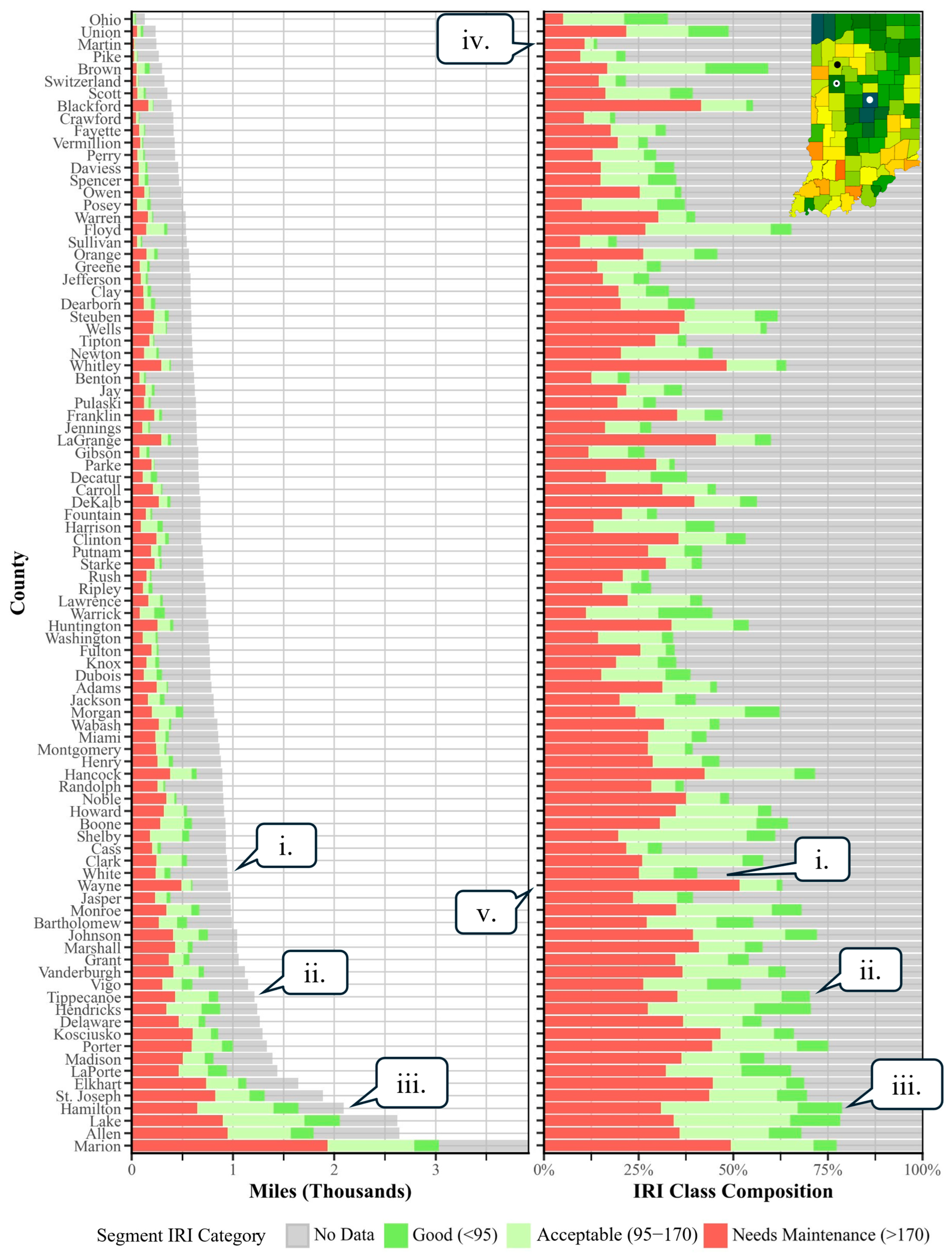
Figure 8 provides a detailed breakdown of paved local roadway conditions across all 92 counties in Indiana, sorted by their mileage. The left panel shows absolute miles by IRI category, while the right panel normalizes these values to display the corresponding composition as a percentage. Together, these figures facilitate both direct comparison across counties and contextual understanding of each county’s network condition.
Each county’s network is classified into the IRI categories of “Good” (<95 in/mi), “Acceptable” (95–170 in/mi), “Needs Maintenance” (>170 in/mi), and “No Data”. Most counties have between 500 and 1000 miles of paved local roadway, but coverage ranges widely from a maximum of 79% in Hamilton County (callout iii.) to a minimum of 14% in Martin County (callout iv.).
This visualization allows for the quick assessment of both the extent and quality of data coverage for any Indiana county and provides insight into how a county compares with other counties of similar network size. County-level roadway condition breakdown figures like Figure 8 can support agency pavement management by aiding the identification of counties with both the greatest need for maintenance and sufficient coverage for informed decision-making, such as Wayne County, where over 50% of the paved local network was categorized as “Needs Maintenance” (callout v.).
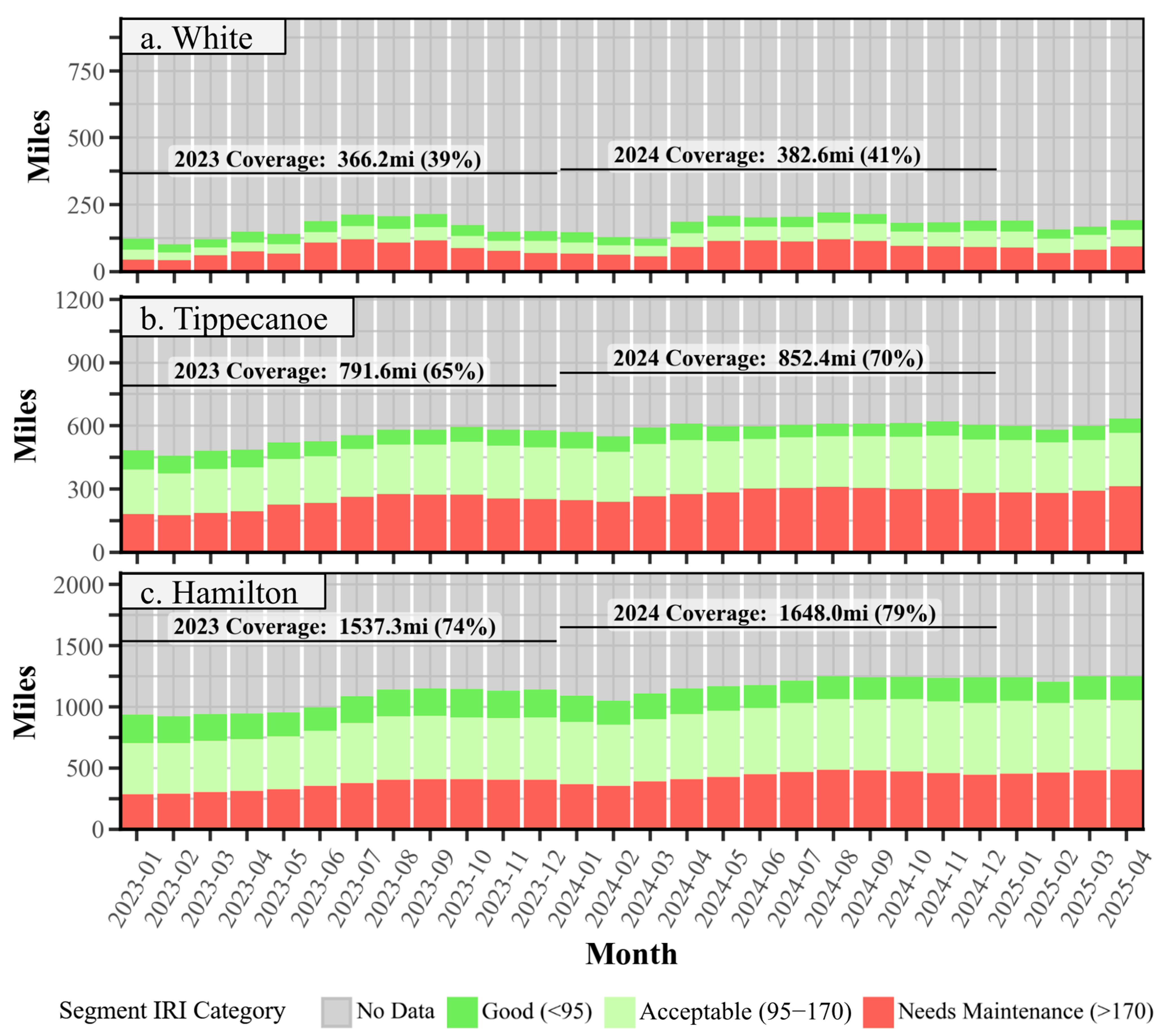
County-level roadway conditions can also be analyzed longitudinally to capture temporal variation. Figure 9 shows the monthly distribution of IRI categories for paved local roads in White (a), Tippecanoe (b), and Hamilton (c) counties over a 28-month period from January 2023 to April 2025. This monthly resolution enables the inspection of seasonal changes in both roadway conditions and data coverage. For example, White County shows noticeably higher data coverage in the summer, which may be explained by seasonal tourists. Additionally, increases in data coverage for Tippecanoe and Hamilton counties are evident. The coverage in both counties increased rapidly from January to August of 2023, which then plateaued.
To illustrate the effect of temporal aggregation, annual coverage lines were added to the figures to highlight how aggregating over a longer time window can significantly improve coverage, typically by about 15% compared to a single month. This increase is due to the accumulation of IRICVe observations over time, where longer periods increase the likelihood of receiving observations for low traffic segments that would otherwise have no data.
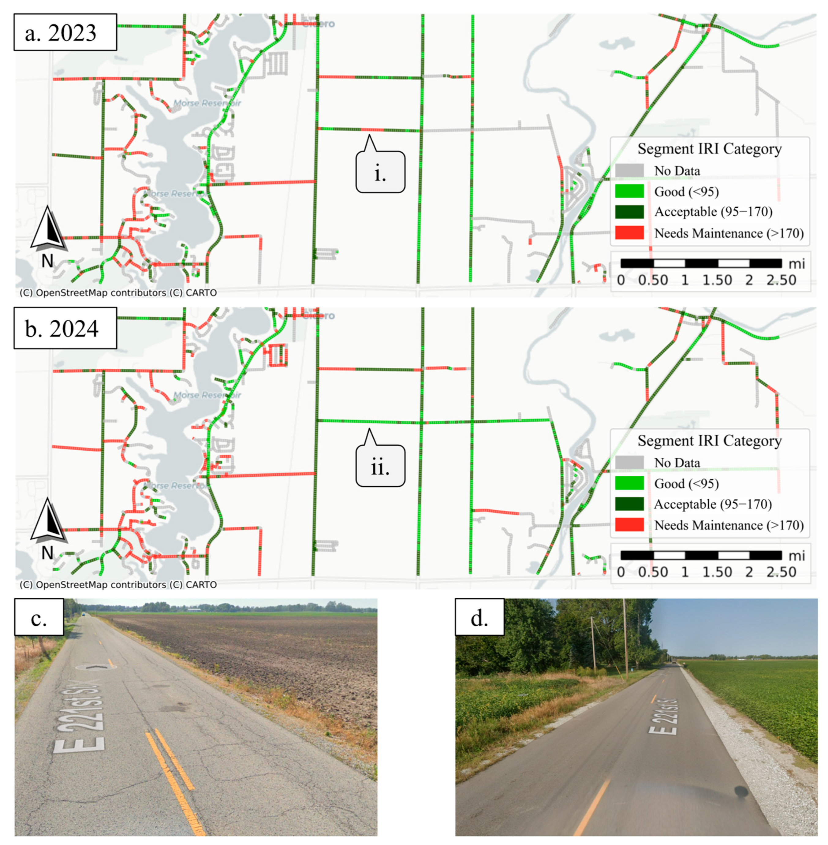
A case study was conducted on a sample of road segments on E 221st street in Hamilton County to demonstrate how IRICVe data can be used for not only broad network-level analysis, but also for high resolution, localized pavement condition monitoring, enabling agencies to detect pavement condition changes with minimal fieldwork. For local agencies, this provides a more scalable alternative to traditional post-maintenance inspection methods.
Figure 10 demonstrates this application using maps of the case study location for both 2023 (a) and 2024 (b). Callouts i. and ii. indicate a target segment that experienced significant IRICVe improvement within one year, decreasing from 221 in/mi to 94 in/mi. This was independently verified with Google Street View imagery of the location in July 2019 (c) and September 2024 (d), which shows the transition from a visibly cracked and deteriorated surface to a newly resurfaced condition in 2024. These findings confirm how roadway maintenance was conducted to improve the surface condition and that the IRICVe data successfully captured the resulting improvement in ride quality.
Although this case study focused on a single location, the same localized analysis can be scaled for proactive network monitoring. By continuously tracking segment-level IRICVe changes over time, agencies can implement automated flagging systems to identify statistically significant improvements or deteriorations. Such change detection algorithms can help prioritize field inspections, verify completed maintenance, and support data-driven decision-making. Notably, roughness change alerts are already offered by some third-party data vendors, making integration into existing workflows feasible without developing additional data-processing infrastructure.

4. Discussion

This study highlights both the potential and current limitations of IRICVe for statewide pavement monitoring. While coverage expanded across Indiana, it remains uneven, with urban counties benefiting from higher CV density and rural areas such as Martin County still experiencing sparse observations.
Differences between interstate, state, and county networks were found, notably that state-managed roads generally have lower IRICVe than local roads (Figure 6). This observation aligns with the higher level of funding for higher volume roads connecting communities [3], while local agencies often face funding challenges [1,2]. By quantifying these differences with IRICVe, agencies gain an objective ride-quality measure that complements distress-based PCI and PASER assessments, which capture distresses that have a negligible impact on roughness.
Temporal analysis (Figure 9) revealed both seasonal and long-term trends. Coverage in White County increased during summer months, likely from visiting traffic associated with local summer recreational sites, while Tippecanoe and Hamilton counties saw substantial growth in 2023 before stabilizing. Annual aggregation improved coverage by about 15% compared to monthly windows, highlighting how agencies can balance temporal precision with data completeness.
The Hamilton County case study (Figure 10) demonstrated how IRICVe can identify maintenance interventions consistent with independent field evidence. Such applications parallel prior validation studies showing that crowdsourced IRI estimates track profiler values within 1–10% [16], and they align with current third-party offerings that can automatically flag changes in pavement roughness [14]. This qualitative evaluation provides empirical evidence suggesting the operational readiness of IRICVe for proactive condition monitoring.
Some limitations remain, however. The dataset is restricted to passenger vehicles [14], meaning that heavy vehicles, which are often the main cause of load-related deterioration, are not accounted for. Prior work shows IRICVe underestimates roughness on deteriorated segments likely because drivers avoid wheel paths with visible distresses [15]. These biases suggest that IRICVe should be interpreted as a conservative estimate of roughness. Coverage in low-traffic counties remains sparse. For example, only 14% of paved local roads in Martin County have data in 2024 (Figure 8). While longer aggregation windows help mitigate data sparsity, IRICVe is not yet a full replacement for profiler surveys on low-volume networks.
These findings support the conclusion that IRICVe is best positioned as a complementary tool within existing asset management workflows. Traditional PCI and PASER surveys remain essential for capturing surface-level distress types such as longitudinal cracking and rutting that do not have a large impact on ride quality [7,8]. Similarly, high-speed inertial profilers remain the preferred data source for project-level investment decisions due to their reliability [9]. IRICVe’s strength lies in providing cost-effective, near real-time screening and prioritization across entire networks that would otherwise be prohibitively expensive.
The broader implication of this study is that CV-based monitoring offers agencies a cost-effective way to obtain a higher resolution and more continuous view of roadway conditions than traditional surveys. By processing terabyte-scale CV data through a transparent, modular workflow, agencies can obtain insight across entire networks at a fraction of the cost of profiler surveys. This framework is not limited to Indiana and can be scaled nationally or adopted by other state agencies. In addition to enabling large-scale predictive maintenance and proactive investment, the approach lowers barriers for smaller jurisdictions and promotes more equitable allocation of resources. These findings illustrate the importance of continued integration with traditional surveys and the exploration of advanced modeling approaches to further strengthen the utility of CV-based monitoring.
Future work will include integrating other data sources such as statewide PASER, PCI, or aggregated trajectory CV data for speed–IRI correlation analysis. To address data sparsity and improve monitoring continuity for low traffic routes, models such as Spatiotemporal Graph Neural Networks (STGNNs) will be explored for data imputation, which have recently demonstrated promising results in prior studies involving CV trajectory prediction and traffic forecasting [29,30].

5. Conclusions

This study presents a modular and robust methodology for large-scale processing and analysis of IRICVe data and evaluates its feasibility for statewide monitoring of local roadway conditions. A detailed data processing pipeline was developed, including base route deduplication, segmentation, buffering, and geospatial data mapping, with transparent explanations of the tradeoffs to support adoption by transportation agencies.
With this pipeline, processed IRICVe data was used to generate visualizations that assess data coverage, condition distributions, and spatiotemporal trends.
  • County-level roughness distributions were compared and provide a high-level overview of the distribution of road roughness across 92 counties and state-managed networks. In this figure, the interstate and state routes are the smoothest, while the county networks are clustered below them, indicating worse conditions.
  • Spatiotemporal trends in data coverage were reviewed. Noteworthy observations include higher data coverage in urban counties and a statewide increase in paved local road coverage from 46.5% to 53.2% between 2023 and 2024, reflecting the growth in OEM CV deployments.
  • County-level IRI category analysis showed variations in road conditions between counties with large and small road networks, seasonal increases in data coverage, and the impact of longer temporal aggregation on data coverage.
  • Coverage increases by roughly 15% for yearly aggregation as opposed to monthly, highlighting the tradeoff between temporal granularity and data coverage when using IRICVe.
  • A localized case study in Hamilton County illustrated the utility of the high spatial granularity of IRICVe. A route segment on E 221st Street showed an IRI improvement from 221 in/mi in 2023 to 94 in/mi in 2024, and maintenance work was confirmed with independent Google Street View imagery. The case study validates the potential of using IRICVe for automated roughness change detection for proactive network screening.
The methodology and findings presented in this study are highly relevant to the asset management workflows of local agencies and provide a strong foundation for transitioning to CV-based condition monitoring at scale.

Author Contributions

Conceptualization, A.T., J.D. and D.M.B.; software, data curation, and validation, A.T. and J.D.; methodology, formal analysis, investigation, and resources, A.T., J.D. and D.M.B.; writing—original draft preparation, A.T.; writing—review and editing, D.M.B. and J.D.; visualization, A.T., J.D. and D.M.B.; supervision, D.M.B.; project administration, D.M.B.; funding acquisition, D.M.B. All authors have read and agreed to the published version of the manuscript.

Funding

This work was supported in part by the Joint Transportation Research Program and Pooled Fund Study SPR-4907, led by the Indiana Department of Transportation (INDOT). The contents of this paper reflect the views of the authors, who are responsible for the facts and the accuracy of the data presented herein and do not necessarily reflect the official views or policies of the sponsoring organizations. These contents do not constitute a standard, specification, or regulation.

Data Availability Statement

The original contributions presented in the study are included in the article, further inquiries can be directed to the corresponding author.

Acknowledgments

The connected vehicle roughness data used in this study was provided by NIRA Dynamics AB. Google Cloud Platform (GCP) and Google BigQuery were used in this study for cloud computing and storage. The authors affirm that no AI or LLMs were used in any capacity in the drafting of the contents of this manuscript. This study is based upon work supported by the Joint Transportation Research Program administered by the Indiana Department of Transportation and Purdue University.

Conflicts of Interest

The authors declare no conflicts of interest.

Abbreviations

The following abbreviations are used in this manuscript:
PCIPavement Condition Index
PASERPavement Surface Evaluation and Rating
IRIInternational Roughness Index
CVConnected Vehicle
IRICVeCV-estimated IRI
IMUInertial Measurement Unit
LiDARLight Detection and Ranging
OEMOriginal Equipment Manufacturer
APIApplication Programming Interface
FHWAFederal Highway Administration
TRBTransportation Research Board
INDOTIndiana Department of Transportation
STGNNSpatiotemporal Graph Neural Network

References

  1. Indiana Local Technical Assistance Program. Local Road & Bridge Condition Report: County/City/Town; Indiana Local Technical Assistance Program: West Lafayette, IN, USA, 2019; Available online: https://www.buildindianacouncil.org/wp-content/uploads/2019/10/LTAP_2019-Local-Road-and-Bridge-Condition-Report-1.pdf (accessed on 23 July 2025).
  2. Applied Pavement Technology, Inc. Indiana Local Roads: An Asset Management Guide for Cities, Towns and Counties; Indiana Local Technical Assistance Program: West Lafayette, IN, USA, 2017; Available online: https://www.asphaltindiana.org/docs/2-LTAP_Asset_Management_Guide.pdf (accessed on 23 July 2025).
  3. Indiana Department of Transportation. Transportation Asset Management Plan (TAMP); Indiana Department of Transportation: Indianapolis, IN, USA, 2022. Available online: https://www.in.gov/indot/files/2022-TAMP.pdf (accessed on 23 July 2025).
  4. National Operations Center of Excellence. Connected Vehicle Data. Available online: https://data.transportationops.org/connected-vehicle-data (accessed on 25 July 2025).
  5. Gopalakrishnan, K. Deep Learning in Data-Driven Pavement Image Analysis and Automated Distress Detection: A Review. Data 2018, 3, 28. [Google Scholar] [CrossRef]
  6. Owor, N.J.; Du, H.; Daud, A.; Aboah, A.; Adu-Gyamfi, Y. Image2PCI—A Multitask learning framework for estimating pavement condition indices directly from images. arXiv 2023, arXiv:2310.08538. [Google Scholar]
  7. ASTM International. Standard Practice for Roads and Parking Lots Pavement Condition Index Surveys (ASTM D6433 20); ASTM International: West Conshohocken, PA, USA, 2020. [Google Scholar] [CrossRef]
  8. Wisconsin Transportation Information Center. PASER Manual: Asphalt Pavement Surface Evaluation and Rating, 2nd ed.; University of Wisconsin–Madison: Madison, WI, USA, 2013; Available online: https://ltap.engr.wisc.edu/wp-content/uploads/2019/12/Asphalt-PASER_02_rev13.pdf (accessed on 23 July 2025).
  9. Federal Highway Administration 2024 Pavements—Inertial Profiler—Pavement (IP). Available online: https://infotechnology.fhwa.dot.gov/inertial-profiler-road-pavement/ (accessed on 23 July 2025).
  10. Abohamer, H.; Elseifi, M.; Dhakal, N.; Zhang, Z.; Fillastre, C.N. Development of a Deep Convolutional Neural Network for the Prediction of Pavement Roughness from 3D Images. J. Transp. Eng. Part B Pavements 2021, 147, 04021048. [Google Scholar] [CrossRef]
  11. De Blasiis, M.R.; Di Benedetto, A.; Fiani, M.; Garozzo, M. Assessing of the Road Pavement Roughness by Means of LiDAR Technology. Coatings 2021, 11, 17. [Google Scholar] [CrossRef]
  12. Justin, M.; Howell, L.; Björn, Z.; Dustin, L.; Darcy, B. Pavement Quality Evaluation Using Connected Vehicle Data. Sensors 2022, 22, 9109. [Google Scholar] [CrossRef] [PubMed]
  13. Mahlberg, J.A.; Li, H.; Zachrisson, B.; Mathew, J.K.; Bullock, D.M. Applications of using connected vehicle data for pavement quality analysis. Front. Future Transp. 2024, 4, 1239744. [Google Scholar] [CrossRef]
  14. Zachrisson, B.; Hägg, J.; Frank, H.; Petersson, J.; Noren, O. Probe vehicle data as input source for road maintenance. In Roads and Airports Pavement Surface Characteristics: Proceedings of the 9th Symposium on Pavement Surface Characteristics (SURF 2022, 12–14 September 2022, Milan, Italy); Crispino, M., Toraldo, E., Eds.; CRC Press: Boca Raton, FL, USA, 2023; pp. 159–167. [Google Scholar] [CrossRef]
  15. Llopis-Castelló, D.; Camacho-Torregrosa, F.J.; Romeral-Pérez, F.; Tomás-Martínez, P. Estimation of Pavement Condition Based on Data from Connected and Autonomous Vehicles. Infrastructures 2024, 9, 188. [Google Scholar] [CrossRef]
  16. Agebjär, M.; Zetterqvist, G.; Gustafsson, F.; Wahlström, J.; Hendeby, G. Road Roughness Estimation via Fusion of Standard Onboard Automotive Sensors. In Proceedings of the 2025 28th International Conference on Information Fusion (FUSION), Rio de Janeiro, Brazil, 7–11 July 2025; Available online: https://www.niradynamics.com/hubfs/FUSION_2025___Nira%205.pdf (accessed on 25 July 2025).
  17. Mathew, J.; Desai, J.; Sakhare, R.; Hunter, J.; Bullock, D. Spatiotemporal Analysis of Pavement Roughness Using Connected Vehicle Data for Asset Management. J. Transp. Technol. 2025, 15, 188. [Google Scholar] [CrossRef]
  18. Mussah, A.R.; Shoman, M.; Amo-Boateng, M.; Adu-Gyamfi, Y. Accelerating statewide connected vehicles big (sensor fusion) data ETL pipelines on GPUs. arXiv 2023, arXiv:2305.07454. [Google Scholar] [CrossRef]
  19. Li, S.; Dragicevic, S.; Castro, F.A.; Sester, M.; Winter, S.; Coltekin, A.; Pettit, C.; Jiang, B.; Haworth, J.; Stein, A.; et al. Geospatial big data handling theory and methods: A review and research challenges. ISPRS J. Photogramm. Remote Sens. 2016, 115, 119–133. [Google Scholar]
  20. National Cooperative Highway Research Program. Guidebook for Data and Information Systems for Transportation Asset Management; The National Academies Press: Washington, DC, USA, 2022; Available online: https://onlinepubs.trb.org/onlinepubs/nchrp/docs/NCHRP08-115FinalReport.pdf (accessed on 25 July 2025).
  21. Purdue University Local Technical Assistance Program. Indiana Local Road and Bridge Report; Purdue University: West Lafayette, IN, USA, 2024; Available online: https://www.purdue.edu/inltap/resources/2024-08-20-Indiana-Local-Road-and-Bridge-Report---FINAL.pdf (accessed on 23 July 2025).
  22. US Roads Dataset. Google Cloud Console. Available online: https://console.cloud.google.com/marketplace/product/united-states-census-bureau/all-roads?hl=en&inv=1&invt=Ab27_Q&project=yt-dl-443015 (accessed on 23 July 2025).
  23. Federal Highway Administration 2024 Office of Highway Policy Information. Available online: https://www.fhwa.dot.gov/policyinformation/pubs/hf/pl11028/chapter7.cfm (accessed on 23 July 2025).
  24. Indiana Geographic Information Office. LRSE Surface Type [Feature Layer]. IndianaMap. Available online: https://gisdata.in.gov/server/rest/services/Hosted/LRSE_Surface_Type/FeatureServer/10 (accessed on 23 July 2025).
  25. Google Cloud. BigQuery Pricing. Google Cloud. Available online: https://cloud.google.com/bigquery/pricing (accessed on 23 July 2025).
  26. Google. BigQuery GeoViz. Google Cloud. Available online: https://bigquerygeoviz.appspot.com/ (accessed on 23 July 2025).
  27. Indiana Geographic Information Office. County Boundaries of Indiana (Current). IndianaMap. Available online: https://www.indianamap.org/datasets/INMap::county-boundaries-of-indiana-current/explore (accessed on 23 July 2025).
  28. Indiana Geographic Information Office. INDOT Districts. IndianaMap. Available online: https://www.indianamap.org/datasets/INMap::indot-districts/explore?location=39.697884%2C-86.424450%2C6.74 (accessed on 23 July 2025).
  29. Gao, Y.; Yang, K.; Yue, Y.; Wu, Y. A vehicle trajectory prediction model that integrates spatial interaction and multiscale temporal features. Sci. Rep. 2025, 15, 8217. [Google Scholar] [CrossRef] [PubMed]
  30. Chen, Y.T.; Liu, A.; Li, C.; Li, S.; Yang, X. Traffic flow prediction based on spatial-temporal multi factor fusion graph convolutional networks. Sci. Rep. 2025, 15, 12612. [Google Scholar] [CrossRef] [PubMed]
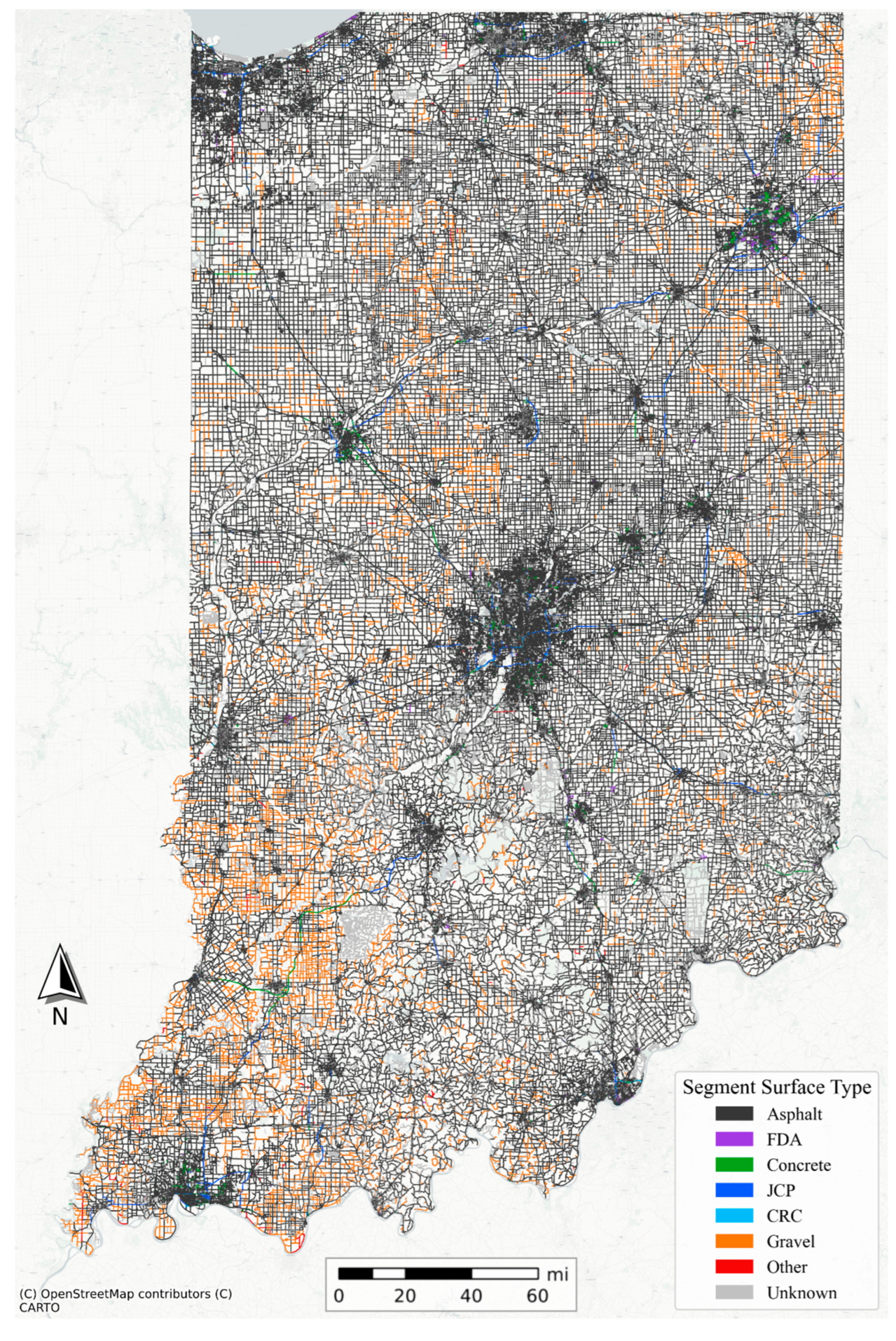
Figure 1. Indiana road network surface type map (2024).
Infrastructures 10 00248 g001
Figure 2. Indiana road network IRI category map (2024).
Infrastructures 10 00248 g002
Figure 3. Route deduplication flowchart.
Infrastructures 10 00248 g003
Figure 4. Route deduplication impact. (a) Before deduplication. (b) After deduplication.
Infrastructures 10 00248 g004
Figure 5. Illustration of data processing steps. Blue is used to represent unmapped geometry. Additional colors in steps d–f represent different IRI categories. In steps g–i they represent distinct surface types.
Infrastructures 10 00248 g005
Figure 6. Segment IRI CFD by interstate, state, and local county roads 2024.
Infrastructures 10 00248 g006
Figure 7. Indiana paved local roads IRI data coverage: (a) 2023; (b) 2024.
Infrastructures 10 00248 g007
Figure 8. IRI category by Indiana county paved local roads (2024).
Infrastructures 10 00248 g008
Figure 9. Paved local roadway IRICVe coverage and IRI categories by month for select counties. (a) White County, (b) Tippecanoe County, (c) Hamilton County.
Infrastructures 10 00248 g009
Figure 10. Hamilton County 9000 block E 221st street case study: (a) 2023 IRI category map, (b) 2024 IRI category map, (c) Google Street View for location i. in July 2019, and (d) Google Street View for location ii. in September 2024.
Infrastructures 10 00248 g010
Disclaimer/Publisher’s Note: The statements, opinions and data contained in all publications are solely those of the individual author(s) and contributor(s) and not of MDPI and/or the editor(s). MDPI and/or the editor(s) disclaim responsibility for any injury to people or property resulting from any ideas, methods, instructions or products referred to in the content.