Article

A Novel Master Curve Formulation with Explicitly Incorporated Temperature Dependence for Asphalt Mixtures: A Model Proposal with a Case Study

by
Gilberto Martinez-Arguelles
1,*,
Diego Casas
2,
Rita Peñabaena-Niebles
3,
Oswaldo Guerrero-Bustamante
4,5 and
Rodrigo Polo-Mendoza
1,6
1
Department of Civil & Environmental Engineering, Universidad del Norte, Barranquilla 080003, Colombia
2
Graduate Program of Water Resources and Environmental Engineering, Federal University of Paraná, Curitiba 80060-000, Brazil
3
Department of Industrial Engineering, Universidad del Norte, Barranquilla 080003, Colombia
4
Department of Civil & Environmental, Universidad de la Costa, Barranquilla 080002, Colombia
5
Construction Engineering Laboratory, The University of Granada (LabIC.UGR), 18071 Granada, Spain
6
Faculty of Science, Charles University, 12800 Prague, Czech Republic
*
Author to whom correspondence should be addressed.
Infrastructures 2025, 10(9), 227; https://doi.org/10.3390/infrastructures10090227
Submission received: 24 June 2025 / Revised: 21 August 2025 / Accepted: 27 August 2025 / Published: 28 August 2025

Abstract

Accurately modelling and simulating the stiffness modulus of asphalt mixtures is essential for reliable pavement design and performance prediction under varying environmental and loading conditions. The preceding is commonly achieved through master curves, which relate stiffness to loading frequency at a reference temperature. However, conventional master curves face two primary limitations. Firstly, temperature is not treated as a state variable; instead, its effect is indirectly considered through shift factors, which can introduce inaccuracies due to their lack of thermodynamic consistency across the entire range of possible temperatures. Secondly, conventional master curves often encounter convergence difficulties when calibrated with experimental data constrained to a narrow frequency spectrum. In order to address these shortcomings, this investigation proposes a novel formulation known as the Thermo-Stiffness Integration (TSI) model, which explicitly incorporates both temperature and frequency as state variables to predict the stiffness modulus directly, without relying on supplementary expressions such as shift factors. The TSI model is built on thermodynamics-based principles (such as Eyring’s rate theory and activation free energy) and leverages the time–temperature superposition principle to create a physically consistent representation of the mechanical behaviour of asphalt mixtures. This manuscript presents the development of the TSI model along with its application in a case study involving eight asphalt mixtures, including four hot-mix asphalts and four warm-mix asphalts. Each type of mixture contains recycled concrete aggregates at replacement levels of 0%, 15%, 30%, and 45% as partial substitutes for coarse natural aggregates. This diverse set of materials enables a robust evaluation of the model’s performance, even under non-traditional mixture designs. For this case study, the TSI model enhances computational stability by approximately 4 to 45 times compared to conventional master curves. Thus, the main contribution of this research lies in establishing a valuable mathematical tool for both scientists and practitioners aiming to improve the design and performance assessment of asphalt mixtures in a more physically realistic and computationally stable approach.

1. Introduction

The stiffness modulus is a rigidity-like measurement for asphalt mixtures at a particular temperature and load frequency [1,2,3]. Thus, the stiffness modulus expresses the level of stress required to produce a given strain, thereby characterizing the material’s ability to sustain mechanical loads [4,5,6]. Although this dependent variable has many interpretations and uses, its most significant application is for the design of pavement structures [7,8,9]. For instance, in the American Association of State Highway and Transportation Officials (AASHTO) 2002 Pavement Design Guide, the stiffness modulus is one of the main variables employed to characterize the mechanical performance of asphalt concretes [7,10]. In order to describe the variations in the stiffness modulus under changes in loading conditions, the master curve concept is typically adopted [11,12,13].
In the literature, a great effort has been made to improve the traditional master curve models, e.g., by considering the influence of the loading rates [14], integrating the relaxation spectrum [15], addressing the effect of the aging depth [4], and including asphalt–filler interaction indices [16]. Nevertheless, there is still no master curve formulation with the temperature explicitly incorporated as a state variable; instead, conventional shift factor expressions are typically employed, e.g., the widely known Arrhenius and Williams–Landel–Ferry (WLF) equations [17,18]. In this regard, the primary aim of this research is to propose a thermodynamically consistent mathematical model to accurately compute the stiffness modulus under specific loading conditions (i.e., frequency and temperature) without resorting to shift functions. This methodological innovation offers a means to simulate the load-bearing capacity of asphalt mixtures without relying on shift factor formulations, whose accuracy and reliability are limited to constrained temperature ranges.
The rest of the document is organized as follows. Section 2 provides background information on conventional master curves and commonly used shift factor formulations. Section 3 details the embraced mathematical modelling framework, integrating thermodynamic principles with the time–temperature superposition principle (TTSP) to develop a novel master curve formulation. Section 4 applies the introduced model to experimental data obtained from recycled concrete aggregate (RCA)-based asphalt mixtures, highlighting the model’s performance and reliability. Section 5 discusses the broader impact of the proposed master curve formulation, including its potential to improve pavement design and analysis, its advantages, calibration requirements, and future research lines. Finally, Section 6 outlines the main conclusions derived from this study.

2. Background

The master curve concept can be applied to almost all viscoelastic materials, particularly those exhibiting both solid-like and liquid-like responses, such as asphalt mixtures, but the asphalt binder, mastic, and mortar can also be modelled through these mathematical expressions [16,19,20]. Thus, it is clear that there is a wide range of applications for master curves. For asphalt mixtures, several master curve formulations have been proposed in the literature, such as the Generalized Sigmoidal (GS) model (Equation (1)), the Canonical Sigmoid (CS) model (Equation (2)), the Standard Logistic Sigmoidal (SLG) model (Equation (3)), and the uniaxial model (Equation (4)) [17,21,22,23]. These formulations, together with more advanced versions, are summarized in Table 1. Likewise, the master curve expressions can equally be employed for other rigidity-like measurements, such as relaxation and the complex modulus (in some cases, mathematical adjustments or physics-based constraints may be required) [24,25,26,27].
l o g 10 E * = δ + α δ 1 + e β + γ l o g 10 f r
l o g 10 E * = α + δ 1 + e β + γ l o g 10 f r
l o g 10 E * = δ + α 1 + e β γ l o g 10 f r
l o g 10 E * = δ + α δ 1 + e β γ l o g 10 f r
where
E* is the stiffness modulus in MPa;
fr is the frequency in Hz;
e is the so-called Euler’s number, a mathematical constant approximately equal to 2.71828;
δ, α, β, and γ are the model-specific fitting parameters.
Table 1. Summary of conventional master curve models along with their advantages and disadvantages.
FormulationsAdvantagesDisadvantagesReferences
GS model
(Equation (1))
These are the most straightforward expressions; their mathematical structure is simple and only requires 4 parameters. Thus, only 4 experimental measurements need to be made for their calibration. This calibration procedure can even be quickly conducted using trial-and-error techniques.These expressions employ frequency as the only state variable, so they cannot reproduce the stiffness dependence on temperature (or other analogous variables) without incorporating shift factors. When the experimental measurements of the stiffness modulus are carried out in a narrow range of frequencies, it is possible for the calibration of the equations to not converge properly.[21,22,23]
CS model
(Equation (2))
SLG model
(Equation (3))
Uniaxial model
(Equation (4))
Generalized logistic sigmoidal model:
l o g 10 E * = δ + α 1 + λ e β γ l o g 10 f r 1 / λ  
Due to the incorporation of an additional fitting parameter (i.e., λ), this model allows adjustment to asymmetric curves.This formulation holds the limitations of the traditional models (Equations (1)–(4)). Compared to traditional models, this formulation requires an additional experimental measurement for its calibration. Inadequate calibration of λ can lead to the construction of unrealistic non-symmetric master curves.[28]
Christensen–Anderson–Marasteanu model:
E * = E e * + E g * E e * 1 + f c f r υ w υ
This model allows the direct specification of the minimum and maximum stiffness moduli through the parameters E e * and E g * , respectively. It permits the high-accuracy reproduction of viscoelastic behaviour.This formulation holds the limitations of the traditional models (Equations (1)–(4)). Also, the trend of the simulated curves depends on one location parameter ( f c ) and two tuning parameters ( υ and w ). Counterintuitively, using few fitting parameters increases the complexity of model calibration because if the experimental data are noisy, the associated error can be increasingly propagated.[29]
Modified Christensen–Anderson–Marasteanu model:
E * = E e * + E g * E e * 1 + ω c E ω a T log 10 ( 2 ) R E R E log 10 ( 2 )
Regarding the original Christensen–Anderson–Marasteanu model, this enhanced version allows the incorporation of the rheological index ( R E ), which can be used as a rotation factor to couple time–temperature–aging shift functions.This formulation holds the limitations of the original Christensen–Anderson–Marasteanu model.[4]
Continuous relaxation spectrum model:
E * = E + + H τ ω 2 τ 2 + i ω τ 1 + ω 2 τ 2 d l n τ H τ = ± 2 π   I m E e ± π 2 i τ E = E + + H τ ω 2 τ 2 1 + ω 2 τ 2 d l n τ
This formulation excels by the incorporation of the continuous relaxation spectrum (through the relaxation time—τ—and angular frequency—ω—parameters) into the calculation of the stiffness modulus. Thus, the model considers the linear viscoelastic properties of asphalt materials. Also, thanks to the use of incremental constitutive relations, the numerical stability of this model is extremely high.As in the traditional formulations (Equations (1)–(4)), this model does not consider the effects of the temperature without incorporating shift factors. Due to the use of multiple integral equations, this model increases its mathematical complexity excessively, which makes its implementation difficult in more extensive simulations. Therefore, the calibration of this model involves the exploration of non-trivial solutions.[15]
Modified Havriliak–Negami model:
E * = E H N + E 0 H N E H N 1 + i ω τ H N α β H N
This model is especially suitable for asphalt mixtures that develop complex liquid-like and solid-like phases throughout the frequency spectrum.This formulation holds the limitations of the traditional models (Equations (1)–(4)). The model is complex both from a mathematical and physical standpoint. On the one hand, this formulation should not be calibrated with a simple iteration for error minimization. On the other hand, the physical interpretation of the fitting parameters is non-intuitive, as is the case with conventional models.[30,31]
Equations (1)–(4) (as well as similar models) share two fundamental characteristics: (i) they relate the stiffness modulus with respect to the frequency, adopting a sigmoidal behaviour with an asymptote at both ends, and (ii) the temperature dependence is not explicitly considered in their formulation. Since these equations do not contain the temperature as a state variable, it is necessary to use shift factors to establish an “equivalence” of the effect that temperature would have on the stiffness modulus based on the influence that frequency has [18,32]. Not considering the temperature in an expression that computes the stiffness modulus is arguably the most significant limitation of the master curve models currently available in the state of the art. Consequently, this investigation effort aims to fill this research gap by developing a novel master curve equation with explicitly incorporated temperature dependence.
In the viscoelastic characterization of asphalt mixtures, shift factors play a central role in the construction of master curves using the TTSP, which is essential for describing the dependence of the stiffness modulus on specific loading conditions (i.e., frequency and temperature) [31]. This procedure enables the condensation of experimental data obtained at different temperatures into a single reference curve, facilitating the prediction of mechanical behaviour under variable loading conditions [27,33]. The process relies on the application of shift factors (hereinafter designated by the term a T ), which quantify the effect of temperature on the viscoelastic response of the material.
Equation (5) illustrates how the TTSP incorporates shift factors to calculate the stiffness modulus at a given frequency and temperature. The procedure is based on calibrating a master curve model at a reference temperature ( T r ). Then, to estimate the stiffness modulus at a target temperature ( T ) and target frequency ( f r ), the calibrated master curve does not use f r directly. Instead, it uses an equivalent reduced frequency ( f r ( T ) ), obtained by multiplying the target frequency ( f r ) by a shift factor specific to the target temperature ( a T ( T ) ). This adjusted frequency reflects how temperature influences the viscoelastic response. At temperatures higher than T r , a T falls within the open interval between 0 and 1, effectively shifting the material behaviour toward lower equivalent frequencies (i.e., softer response). In contrast, at temperatures lower than T r , a T should be greater than 1, shifting the behaviour toward higher equivalent frequencies (i.e., stiffer response). In this way, the TTSP enables the prediction of mechanical response across a range of temperatures using a single calibrated master curve. The critical challenge lies in accurately determining a T values, as incorrect values can lead to significant errors in the predicted stiffness modulus.
f r ( T ) = f r a T ( T )
Two of the most widely used a T are the Arrhenius model (Equation (6)) [34,35,36] and the WLF model (Equation (7)) [17,37,38]. These models facilitate the construction of master curves by calculating shift factors that adjust the effective frequency as a function of temperature. On the one hand, the Arrhenius equation describes the thermal dependence of viscoelastic materials in the glassy regime, where relaxation processes are dominated by thermally activated mechanisms [35,36]. This model is suitable for describing the behaviour of asphalt-based materials at temperatures below the glass transition ( T g ), where molecular mobility is limited and the response is predominantly elastic and brittle [39]. However, its applicability decreases near or above T g , where the linearity of the thermal dependence is lost and the material transitions to a more ductile state. On the other hand, the WLF equation is widely used for amorphous polymers and asphalt-based materials near T g , capturing the nonlinearity associated with the increase in the molecular free volume. The WLF equation is especially accurate near and above T g but loses validity in the deep glassy regime, where the thermal dependence is better described by the Arrhenius model [39,40].
l o g 10   a T = E a 2.303 R 1 T 1 T r
l o g 10   a T = C 1 T T r C 2 + T T r
where
T is a given temperature in K;
T r is the reference temperature in K;
a T is the shift factor at T relative to the T r ;
R is the universal gas constant, i.e., approximately 8.314 J/mol·K;
E a is the activation energy (in J/mol), used as an empirical constant to represent the energy barrier associated with molecular mobility;
C 1 is a dimensionless empirical constant;
C 2 is an empirical constant in K.
Recent research has proposed alternatives such as the log-linear and quadratic polynomial equations, which can improve the fit of shift factors over wide temperature ranges or in mixtures with modifiers and/or recycled materials [17,39,41]. Additionally, the Kaelble equation, based on WLF, has demonstrated greater symmetry and accuracy for describing thermal dependence below T g [38,41]. Table 2 presents a summary of these shift factor models, highlighting applicability and limitations. As shown in Table 2, T g is a critical parameter that delineates the applicability regimes of these models. In asphalt binders, T g typically ranges from −40 °C to 0 °C for virgin binders and can increase with aging or chemical modification [17,42,43]. In asphalt mixtures, the presence of aggregates and fillers can elevate T g to values between −30 °C and 10 °C, depending on mixture composition and oxidation degree. Correct identification of T g is essential for selecting the most appropriate shift factor model and avoiding erroneous extrapolations [17,42,43,44].
Despite their utility, classical shift factor models present important limitations. Arrhenius assumes a constant activation energy, which does not reflect the compositional heterogeneity or phase transitions present in complex asphalt mixtures, especially those with high recycled material and/or additive content [34,35]. WLF depends on empirical constants that require specific calibration for each mixture; also, its validity is restricted to a limited range around T g . Both models treat temperature indirectly, presupposing a perfectly straightforward equivalence between temperature and frequency, which may not hold in non-thermo-rheologically simple materials or under accelerated aging [46,47]. The need to switch models according to the thermal regime (glassy vs. rubbery) complicates practical application in pavements subject to extreme climatic variations.
The recent literature emphasizes the need for advanced master curve models that outperform existing ones by, for example, explicitly incorporating temperature as a state variable, reducing reliance on shift factors, and enhancing predictive robustness across the full thermal spectrum [3,48,49]. In this sense, approaches such as the one proposed in this study represent an advance by directly integrating thermodynamic principles, eliminating the need for supplementary shift factors and enabling a more stable and physically meaningful representation of the stiffness modulus. Thus, it is possible to offer greater consistency even for asphalt mixtures with unconventional compositions, contributing to more resilient pavement design under evolving climate scenarios.

3. Mathematical Modelling

A mathematically staged approach is followed to develop a master curve formulation with explicitly incorporated temperature dependence. This approach is composed of two stages. The first and second ones are the rationalization and refinement stages, respectively.
Firstly, in the rationalization stage, logical reasoning is performed to model the asphalt mixtures’ viscoelastic behaviour. In this regard, it is essential to highlight two well-known mechanical principles. On the one hand, the viscoelasticity (i.e., the time-dependent response) of asphalt materials implies higher stiffness at higher loading frequencies [15,28]. On the other hand, the associated frequency–stiffness curves are shifted down as the temperature increases, which means lower stiffness at higher loading temperatures [30,31]. Although both temperature and frequency influence stiffness through distinct mechanisms, their combined effect can be meaningfully approximated by considering additive contributions. This approach provides a flexible structure for capturing the main features of the viscoelastic response while preserving interpretability. In order to reflect the interaction between these two state variables, shared fitting parameters should be employed, linking the temperature- and frequency-triggered terms. This calibration strategy helps ensure a synergistic response that avoids overprediction. Thus, it is proposed in Equation (8) that the stiffness modulus ( E * ) can be computed as the sum of two parts, namely, the temperature-triggered stiffness ( E T * ) and frequency-triggered stiffness ( E f r * ).
E * = E f r * + E T *
Secondly, in the refinement stage, E f r * and E T * are defined. On the one hand, E f r * can be adopted as any of Equations (1)–(4). It is essential to highlight that, for Equations (1)–(4), the fitting parameters (δ, α, β, and γ) vary for each model, even when the experimental data correspond to the same asphalt mixture at a specific temperature [23,50]. The preceding is because each mathematical expression (despite being slightly similar) exhibits a distinct pattern for each parameter [51,52,53]. Regardless, those models are interchangeable with each other since they share the same sigmoidal-like mathematical logistic nature. Hence, this research adopts the GS model (Equation (1)) to define E f r * . The chosen model, while comparable in algebraic structure and predictive capabilities to its counterparts (such as the CS, SLG, and uniaxial models), was selected for its established precedence in the literature as a foundational basis for further innovations [21].
Thus, the stiffness modulus from Equation (1) is isolated to obtain a more user-friendly expression, yielding Equation (9). Also, it is worth noting that numerically fitting the logarithms of f r and E * , instead of f r and E * directly, may result in large deviations towards the asymptotic tails of the sigmoid curve.
E f r * = 10 δ + α δ 1 + e β + γ l o g 10 f r
In order to define E T * , thermodynamics-based principles and the TTSP are employed. Initially, it is necessary to recall Eyring’s rate theory, as expressed in Equation (10) [54,55]. Eyring’s rate theory explains molecular rearrangement as a thermally activated process, governed by the principles of statistical thermodynamics [55,56]. It provides a direct link between molecular kinetics and macroscopic properties by relating the transition rate to the energy required to overcome a potential barrier [57,58]. Equation (10) expresses the transition rate ( r ), which is equivalent to frequency, as a function of the absolute temperature ( T ), Boltzmann constant ( k B , i.e., 1.380649 10 23   J / K ), and activation free energy ( Δ G ), which itself combines the effects of activation enthalpy ( Δ H ) and activation entropy ( Δ S ) as Δ G = Δ H T Δ S [59,60]. The term r 0 represents the attempt frequency or pre-exponential factor, indicating the intrinsic rate of molecular vibrations [54,61]. This formulation is a simplified and widely used version of Eyring’s base equation, isolating the temperature dependence in the exponential term to describe the likelihood of molecular transitions over an energy barrier [60,62]. In the context of asphalt mixtures, this equation is particularly relevant because it enables the modelling of temperature-dependent mechanical behaviour by capturing the effect of thermal activation on the rearrangement of molecular structures within the asphalt matrix. As asphalt mixtures behave like a viscoelastic material [63,64,65], the ability to relate frequency to temperature through activation energy provides a physically grounded method for simulating their response under varying thermal and rate conditions.
r = r 0 e Δ G k B T
For asphalt mixtures, Eyring’s rate theory allows the transition rate of molecular rearrangements to be directly represented by a loading frequency ( f r ) because each thermally activated event corresponds to a discrete structural shift contributing to deformation. Since these transitions are driven by thermal energy and occur at a rate proportional to their frequency, no further modifications are needed when modelling viscoelastic behaviour. This simplification holds as long as each crossing over the energy barrier results in an irreversible or statistically significant microstructural change. So, Equation (10) can be reformulated into Equation (11).
f r = f r 0 e Δ G k B T
Now, the activation free energy is written in terms of the activation enthalpy and activation entropy. Thus, from Equation (11), Equation (12) is derived.
f r = f r 0 e Δ S T Δ H k B T
The exponential term in Equation (12) can be simplified, yielding Equation (13).
f r = f r 0 e Δ S k B Δ H k B T
Taking decadic logarithms on both sides of Equation (13), it is possible to obtain Equation (14).
log 10 ( f r ) = log 10 ( f r 0 ) + Δ S k B Δ H k B T log 10 ( e )
Equation (14) can be further rewritten as Equation (15).
log 10 ( f r ) = log 10 f r 0 + Δ S log 10 e k B Δ H log 10 e k B T 1
Equation (15) comprises two constants (i.e., log 10 e and k B ) and three material-dependent fitting parameters (i.e., f r 0 , Δ S , and Δ H ). These constants and material-dependent fitting parameters can be consolidated into two new calibration parameters, ψ and χ , giving rise to Equation (16). In order to avoid ambiguities, Equations (17) and (18) clarify the definitions of ψ and χ .
log 10 ( f r ) = ψ χ T 1
ψ = log 10 f r 0 + Δ S log 10 e k B
χ = Δ H log 10 e k B
Now, Equation (16) can be embedded into Equation (1) (i.e., the GS model, which was adopted as E f r * ), thus leading to a new expression, Equation (19). This integration is grounded in the TTSP, which is a well-established approach widely used in the numerical modelling of asphalt-like materials (e.g., asphalt binders and asphalt mixtures) [66,67,68,69]. The TTSP assumes that frequency and temperature have coupled effects on the material’s response and can be related through mathematical formulations. Thus, by combining the TTSP with thermodynamics-based principles, it is possible to replace the frequency with a temperature-dependent expression. The main advantage of this TTSP implementation is its generalization, as it applies to any temperature, without being confined to a specific range, in contrast to shift factors, whose validity predominantly relies on proximity (or distance) to the T g .
l o g 10 E * = δ + α δ 1 + e β + γ ψ γ χ T
Again, the stiffness modulus from Equation (19) is isolated to obtain a more user-friendly expression, yielding Equation (20). It is important to highlight that the stiffness modulus is denoted as E T * in Equation (20), since the temperature is the only state variable contained in this expression.
E T * = 10 δ + α δ 1 + e β + γ ψ γ χ T
Equation (20) has a notable shortcoming, i.e., the exponential function governing the temperature sensitivity can produce abrupt changes in the mechanical response, resulting in a curve/surface that may lack smoothness and fail to (accurately) represent the gradual relaxation behaviour observed in asphalt mixtures. In order to correct this flaw, a new calibration parameter (i.e., ϕ ) is introduced, leading to the development of Equation (21).
E T * = 10 δ + α δ 1 + e β + γ ψ γ χ T / ϕ
Finally, Equations (9) and (21) are combined into Equation (8) to form Equation (22). Thus, Equation (22) is the proposed master curve formulation with explicitly incorporated temperature dependence. Hereinafter, this is called the Thermo-Stiffness Integration (TSI) model. Basically, the TSI model comprises two terms. The first and second terms are the frequency-triggered stiffness and the temperature-triggered stiffness, respectively.
E * = 10 δ + α δ 1 + e β + γ l o g 10 f r + 10 δ + α δ 1 + e β + γ ψ γ χ T / ϕ
where
E* is the stiffness modulus in MPa;
fr is the frequency in Hz;
T is the temperature in K;
e is the so-called Euler’s number, a mathematical constant approximately equal to 2.71828;
δ ,   α ,   β ,   a n d   γ are the (original) fitting parameters related to the frequency;
ψ ,   χ , a n d   ϕ are the (new) fitting parameters related to the temperature.
Regarding the GS model (Equation (1)), the TSI model (Equation (22)) introduces 3 new fitting parameters associated with thermal effects, namely, ψ , χ , and ϕ . ψ and χ are fitting parameters related to the activation entropy and activation enthalpy, respectively. Meanwhile, ϕ is a fitting parameter that modulates the rate at which the logistic function transitions. Thus, ϕ allows the model to capture more realistic thermo-rheological behaviour, where the influence of temperature evolves progressively rather than instantaneously. Additionally, the ϕ parameter introduces asymmetry into the model by controlling the rate of transition in the E T * term, effectively allowing the curvature to stretch or compress unevenly across the frequency spectrum. This flexibility is particularly valuable for asphalt mixtures, as their viscoelastic behaviour often deviates from ideal symmetry due to factors like polymer modification, aging, and/or the presence of additives that alter relaxation characteristics. Although these parameters have a physical meaning coupled to temperature, they should only be obtained by calibrating experimental data. In this way, the calibrated parameters accurately reflect the actual thermomechanical behaviour of a specific asphalt mixture.

4. Case Study

4.1. Materials

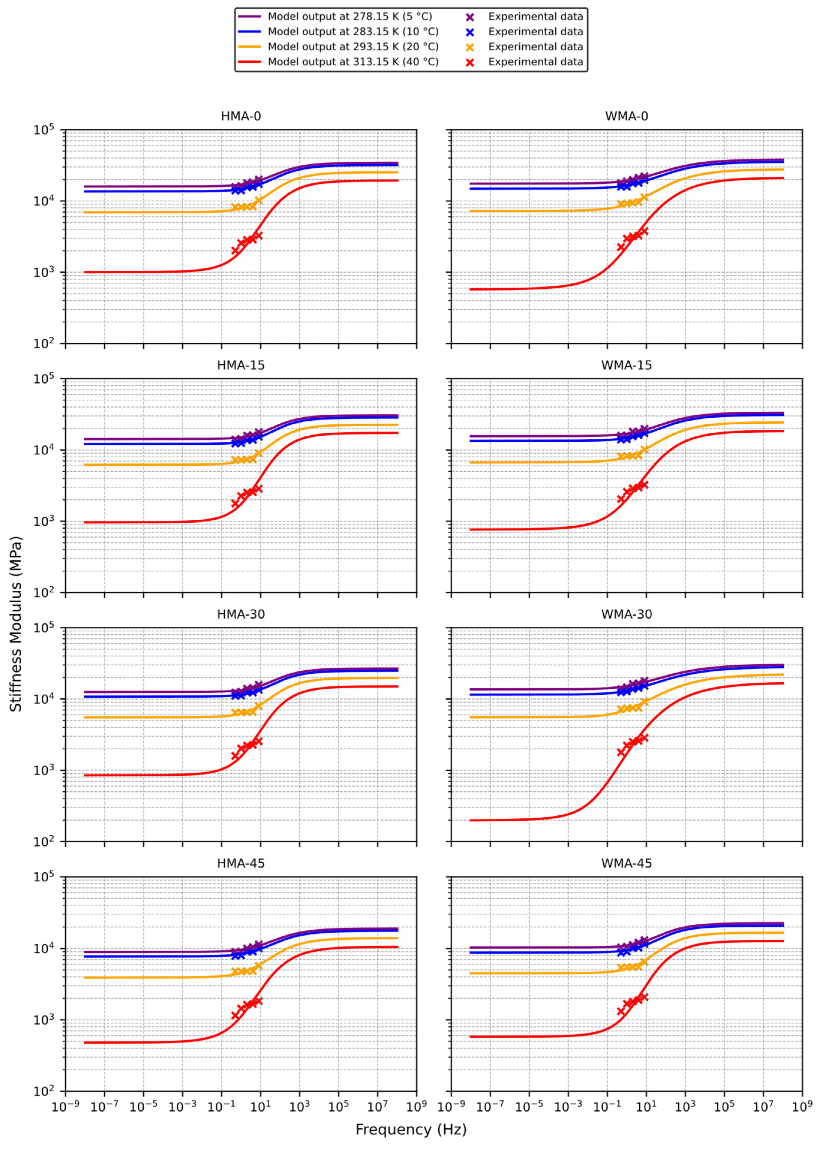
A case study is analysed herein to evaluate the proposed TSI model’s efficacy. For this purpose, the experimental data reported by Covilla-Varela et al. [70] are adopted. That investigation studied RCA-based asphalt mixtures. Thus, eight mixture designs are considered from [70], which comprise four hot-mix asphalts (HMAs) and four warm-mix asphalts (WMAs). For both types of asphalt concretes, there are designs with 0, 15, 30, and 45% coarse RCA as a partial replacement of coarse natural aggregates (NAs). Table 3 shows the gravimetric composition and laboratory characterization of these asphalt mixtures. Figure 1 exhibits the experimentally measured stiffness modulus for each asphalt mixture. It is important to highlight that the stiffness moduli were obtained for 20 different loading conditions, i.e., the combination of 5 frequencies (0.5, 1, 2, 4, and 8 Hz) and 4 temperatures (5, 10, 20, and 40 °C).
Below is a brief description of the origin of the raw materials used to produce the analysed asphalt mixtures. First, a 60/70 penetration-grade asphalt binder was used as the base binder. For the WMAs, the base binder was modified with a chemical additive (Iterlow T) at a dosage of 0.3% by asphalt binder weight. The NAs were extracted from a quarry in the Department of Atlántico (northern region of Colombia); this quarry is mainly composed of sedimentary rocks of marine origin. Finally, the RCAs were obtained by demolishing and crushing several recently constructed Portland cement concrete slabs, which were designed to develop a flexural strength (the so-called modulus of rupture) of 3.8 MPa. More detailed information can be found in [70,71].

4.2. Results

The trust-region-reflective algorithm was employed to calibrate the TSI model (Equation (22)) for the experimental values previously introduced (Figure 1). This algorithm is a robust optimization procedure used for fitting data, and its execution requires bounds and initial values [72,73,74]. For this research, the bounds refer to the extreme possible values of the fitting parameters, which were assumed to be between −1000 and 1000. Figure 2 shows the obtained outcomes.
Figure 2 shows the calibration of the TSI model for the HMAs and WMAs. This graph clearly indicates that the proposed master curve formulation can reproduce the mechanical behaviour of the asphalt mixtures. As expected, the TSI model obeys the following trends: (i) the stiffness increases with increasing frequency; (ii) the stiffness decreases with increasing temperature; (iii) there are realistic values for the two asymptotic tails; and (iv) smooth changes occur at all points of the curves without sudden or abrupt gradients. Table 4 presents the fitting parameters obtained from the calibration procedure. This table also discloses a basic statistics description of these fitting parameters; it includes the minimum, maximum, average, median, standard deviation, skewness, and kurtosis values. Table 4 exhibits two goodness-of-fit parameters to evaluate the accuracy of the modelled stiffness moduli, i.e., the coefficient of determination (R2, according to Equation (23)) and Mean Absolute Percentage Error (MAPE, according to Equation (24)). The TSI model demonstrates excellent accuracy, with R2 values consistently exceeding 0.98 and MAPE values remaining below 8.5%. These results confirm that the TSI model provides a highly precise fit to the experimental data, reliably capturing the material behaviour across the evaluated loading conditions. From Figure 2 and Table 4, it is evident that the TSI model successfully manages to overcome the two main shortcomings associated with the traditional master curve models, i.e., the temperature dependence is explicitly incorporated, and the equation offers excellent stability despite being calibrated with a narrow range of frequencies. These essential improvements are due to the integration of the temperature-related sigmoidal term (i.e., the second term in Equation (22)).
Table 4. Outcomes of the TSI model for the addressed case study.
Fitting ParametersAccuracy
α β γ δ ψ χ ϕ R 2 (-)MAPE (%)
Asphalt
Mixtures
HMA-02.457944−0.5910821.1038024.2710440.523182−3.7210080.0003750.99207.34
HMA-152.452728−0.7318211.1970444.2220300.599018−3.7250210.0004100.99177.37
HMA-302.418613−0.7150551.1692344.1593720.599273−3.7058050.0003830.99167.21
HMA-452.140254−0.3993501.0332274.0084990.374255−3.7046190.0003300.99057.90
WMA-02.0584950.1272870.7742474.317418−0.176631−3.7214310.0002660.99376.73
WMA-152.332162−0.2475390.9063084.2538950.260827−3.7200970.0002920.99237.09
WMA-300.9389640.7699650.6435734.225295−1.208403−3.7168410.0002440.99127.86
WMA-452.147436−0.4492151.1000284.0899460.396154−3.7051440.0003920.98958.48
Statistical
Description
Minimum0.938964−0.7318210.6435734.008499−1.208403−3.7250210.000244
Maximum2.4579440.7699651.1970444.3174180.599273−3.7046190.000410
Average2.118325−0.2796010.9909334.1934370.170959−3.7149960.000337
Median0.8544650.7067692.6027722.303886−2.456511−1.8521880.000353
Std0.4688900.4746610.1855650.0954950.5716560.0078800.000059
Skewness−2.3094641.474897−0.865064−0.863506−2.0405990.388598−0.386632
Kurtosis5.8015661.973254−0.4863270.0665874.247876−2.042569−1.667467
Abbreviations: Std—standard deviation.
M A P E = 100 % n i = 1 i = n O D i E D i O D i
R 2 = 1 i = 1 i = n O D i E D i 2 i = 1 i = n O D i i = 1 i = n O D i n 2
where
n is the number of experimental points, i.e., 20;
i is an index that traverses from 1 to n ;
O D i is an original/experimental data point;
E D i is an estimated data point.
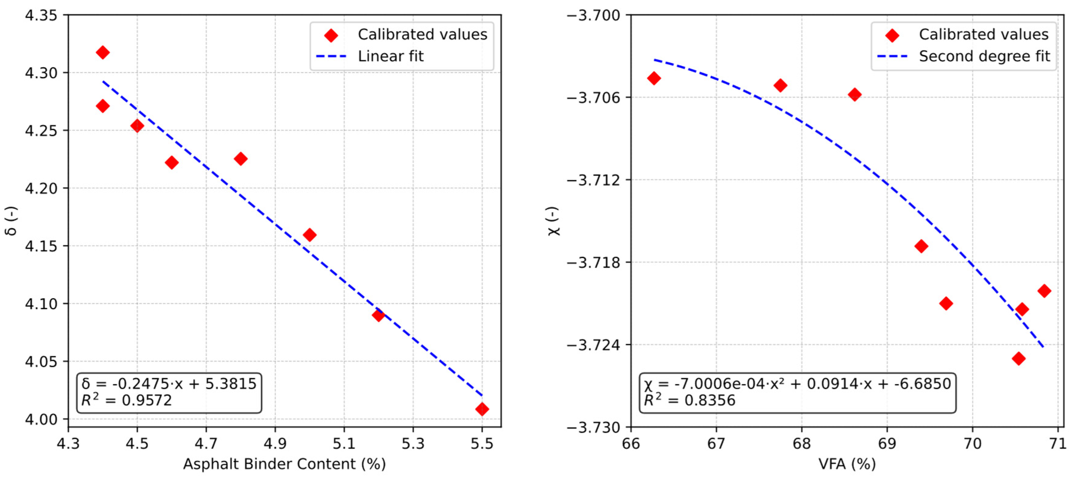
Notably, two fitting parameters of the TSI model (i.e., δ and χ ) exhibit strong correlations (R2 > 0.8) with key mixture properties. As illustrated in Figure 3, δ correlates significantly with the asphalt binder content, while χ shows a strong relationship with the VFA. In contrast, the remaining fitting parameters do not display such strong associations. This observation is particularly relevant given that the TSI parameters have meaningful physical interpretations tied to mixture design. Further research is warranted to explore this aspect in greater depth, particularly by calibrating the TSI model across a broader range of asphalt mixtures to investigate the potential existence of additional correlations.
A plausible hypothesis for the observed correlation between the fitting parameter χ , related to activation enthalpy, and the VFA may lie in the microstructural dynamics governing molecular mobility within the asphalt matrix. As the VFA increases, the proportion of the aggregate matrix saturated by the asphalt binder also rises, potentially reducing the free volume available for molecular rearrangement. This reduction could affect the strength of intermolecular interactions or the density of local binding sites, which in turn may alter the enthalpic barrier required for thermally activated transitions such as viscous flow or phase rearrangement. Thus, the parameter χ could reflect the ease with which molecular chains overcome energy barriers under thermal activation, a process intrinsically tied to the degree of binder saturation in the void structure. Moreover, χ arguably controls how the binder–aggregate microenvironment impacts energy dissipation mechanisms. Since this reasoning is grounded in qualitative microstructural behaviour and not directly validated through experimental mechanistic evidence, further studies using techniques such as molecular dynamics simulations or advanced rheo-physical characterization are necessary to confirm this hypothesis.

5. Discussion

5.1. Convergence Challenges

One of the aspects that most influence the numerical calibration of complex mathematical models is the setting of initial values [75,76,77]. Initial values are the starting points of most error-minimization methods and even for exploration–exploitation search space algorithms [78,79]. In this regard, the greater the distance between the initial and optimal values, the greater the running time and memory usage, and even non-convergence may occur in particular cases [80,81].
In order to ensure the effective implementation of the TSI model, the following recommendations can assist in selecting appropriate initial values during calibration. A straightforward and practical option is to use any of the parameter sets listed in Table 4, which guarantees that the model begins with physically meaningful behaviour. Alternatively, the average values of those parameters, also provided in Table 4, offer a reliable starting point. These choices are generally interchangeable and do not introduce additional complexity into the calibration process. Nonetheless, the specific selection may have a significant impact in particular contexts, such as when the TSI model is embedded in iterative computational procedures (e.g., finite element or discrete element simulations) or applied to highly modified asphalt mixtures exhibiting atypical viscoelastic responses.
In order to prove the high computational stability of the proposed TSI model (Equation (22)), it was benchmarked against the traditional master curve models (Equations (1)–(4)). For this purpose, all five models were independently calibrated using a Python-based script across the eight considered asphalt mixtures. For each mixture and each of the evaluated models, 1000 independent optimization executions were performed, totalling 8000 runs per master curve. In every execution, the initial parameter values were randomly generated from a uniform distribution ranging from −100 to 100. Table 5 presents the number of non-convergent runs per mixture and per model, allowing a clear comparison of robustness. A run was classified as non-convergent when the calibration using the trust-region-reflective algorithm failed, which was defined by at least one of the following conditions: (i) the algorithm exceeded the maximum number of function evaluations, which was set to 10,000, or (ii) a mathematically impossible operation occurred, such as division by zero, generation of undefined numerical values, use of singular matrices, or other forms of numerical instability. For a given asphalt mixture, the TSI model was calibrated over the entire dataset of loading conditions (i.e., 20 data points resulting from the combination of 4 temperatures and 5 frequencies). Conversely, the traditional models were calibrated independently at each temperature level, so a run was marked as non-convergent if at least one temperature-specific sub-calibration failed.
Table 5 presents the total number of non-convergent runs and presents the percentage of failures relative to the total of 8000 runs per model. While all models showed overall strong stability with failure rates under 2%, differences between them were substantial. The SLG model was the least stable, with 1.79% non-convergence, followed by the CS model at 1.73%, the uniaxial model at 0.23%, the GS model at 0.16%, and finally the TSI model, which had just 0.04% non-convergence. Table 5 also reports the ratio between each traditional model’s failure rate and that of the TSI model, showing that the TSI is approximately 45 times more stable than the SLG model, 43 times more than the CS model, 6 times more than the uniaxial model, and 4 times more than the GS model. Several insights arise from these results. Firstly, the TSI model addresses a key limitation of conventional master curves, which often struggle with convergence when experimental data is limited to a narrow frequency range. Secondly, among the four traditional models, the GS model demonstrated the highest stability, which reinforces its selection as the foundation for the development of the TSI model. Although this improvement in convergence reliability may appear modest, it becomes highly relevant in large-scale computational applications, such as finite element or discrete element simulations, where automated verification of calibration reliability is not always feasible. It is important to emphasize that these findings are based on a single case study, and future in-depth research is necessary to further validate and refine these conclusions.
The high computational stability of the TSI model, as demonstrated in Table 5, can be attributed to two main factors. On the one hand, the TSI model was developed based on the GS model, which, among the evaluated traditional master curve formulations, exhibited the highest numerical stability. This foundational choice provided the TSI model with a solid starting structure already proven to be robust under a wide range of calibration conditions. On the other hand, the TSI model introduces structural enhancement by decomposing the prediction of the stiffness modulus into the sum of two independent sigmoidal components. This decomposition enables a more localized fitting response, thereby reducing the likelihood that convergence issues or sensitivity to initial parameter values will impact the entire model simultaneously. In scenarios where one sigmoidal term encounters numerical challenges, such as poor parameter initialization or limited information in a specific range of the dataset, the other term can still provide a valid contribution to the predicted modulus. This built-in redundancy enhances robustness during nonlinear optimization, helping the algorithm avoid stagnation in flat or ill-conditioned regions of the solution space. By distributing the modelling process between two coordinated components, the TSI model achieves a more stable and flexible formulation that improves the likelihood of successful convergence across diverse calibration scenarios.

5.2. Benchmarking Against the Traditional Approach

In order to perform a comparison of the proposed TSI model against the traditional approach, a benchmarking prediction of the stiffness modulus for the addressed case study is presented using the GS model to calibrate the master curves (of each asphalt mixture) at a reference temperature of 20 °C while applying both the Arrhenius and WLF formulations to derive the corresponding shift factors for the other considered temperatures (i.e., 5, 10, and 40 °C). Both shift factor expressions were applied because the laboratory data for these mixtures did not include the T g , making it impossible to presume in advance which equation was more appropriate. The GS model was selected not only because it represents the foundational structure upon which the TSI model was developed but also due to its superior numerical/computational stability compared to the other conventional alternatives evaluated in the study (see Table 5).
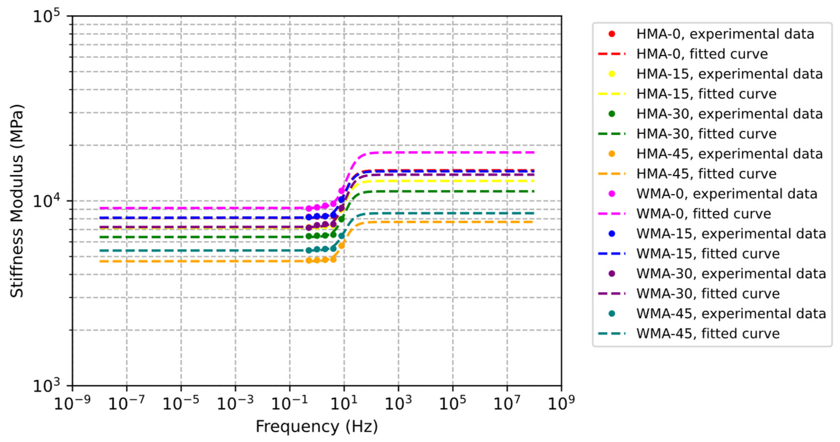
Table 6 presents the fitting parameters obtained for the eight asphalt mixtures calibrated at 20 °C using the GS model. Figure 4 illustrates the resulting master curves alongside the corresponding experimental data. Additionally, Table 7 summarizes the empirical constants associated with the Arrhenius and WLF models. Finally, Table 8 displays the a T values calculated for each asphalt mixture using both shift factor formulations.
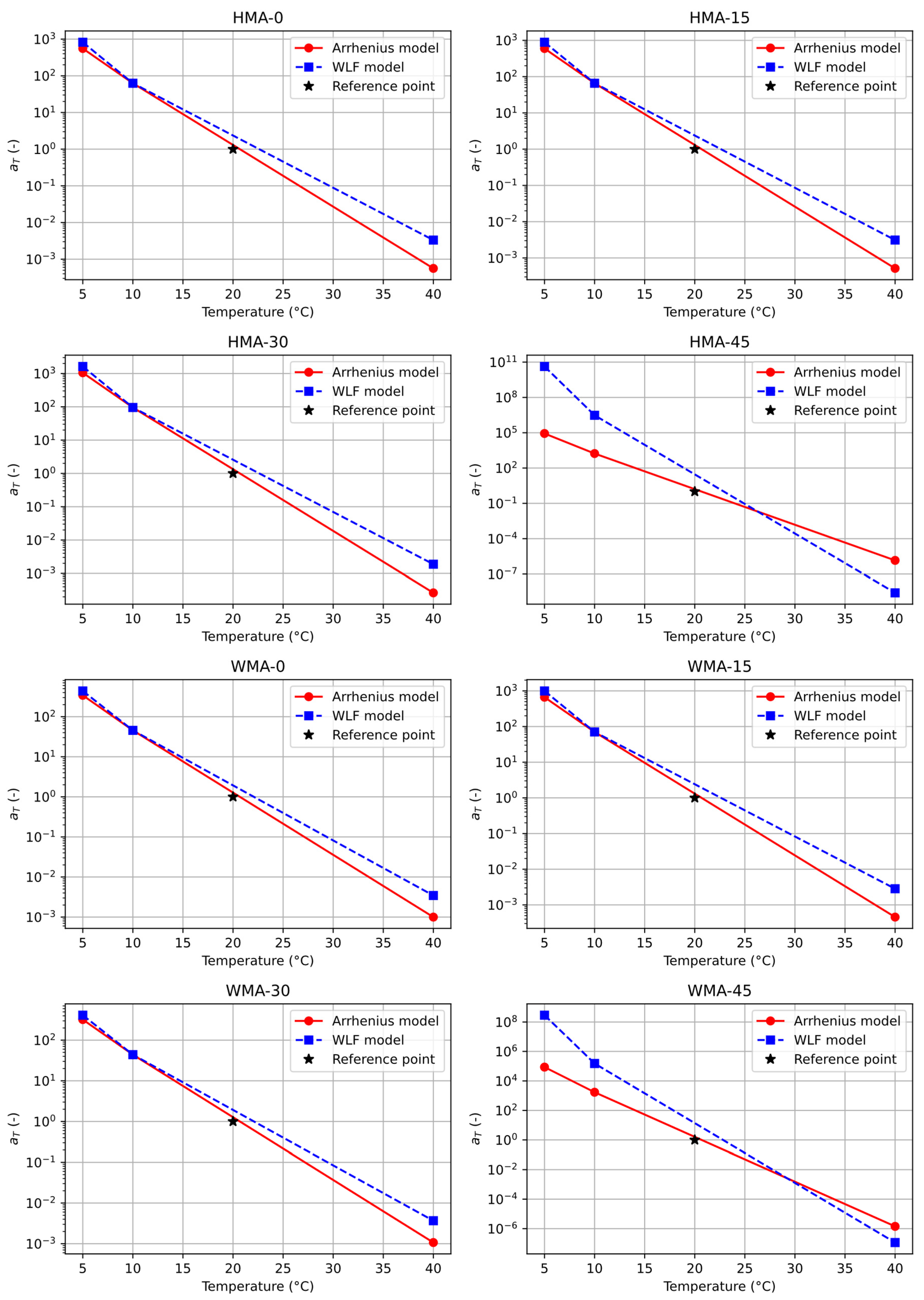
The calibrated empirical constants presented in Table 7 were obtained by minimizing the MAPE between the predicted and experimental values, ensuring the most accurate possible estimation of a T . In order to assess the reliability of each shift factor formulation, a graphical inspection is necessary. Figure 5 illustrates the evolution of a T across target temperatures (i.e., 5, 10, and 40 °C) for each asphalt mixture. In each sub-plot, the x-axis represents temperature on a linear scale, while the y-axis displays a T on a logarithmic scale. A reference point is also included, corresponding to an a T equal to 1 at the reference temperature of 20 °C. Two graphical criteria are used to evaluate the performance of these expressions. Firstly, the trajectory of the lines should follow a near-linear trend due to the scaling of the axes. Secondly, the reference point should align with the overall trend of each line. Based on these observations, Figure 5 clearly indicates that the Arrhenius model provides a more reliable representation of temperature-dependent shift behaviour for the asphalt mixtures evaluated in this study.
Some of the resulting shift factors (shown in Table 8 and Figure 5) appear to deviate notably from values that are typically expected in practice. Thus, it is necessary to perform a more detailed inspection of this traditional approach. In this regard, Table 9 reports MAPE values calculated between experimental values and model predictions. For a reference temperature of 20 °C, predictions were based on the GS model. For the target temperatures (i.e., 5, 10, and 40 °C), the MAPE was computed using both the Arrhenius and WLF formulations. Several important observations can be drawn from this benchmarking. Firstly, although the Arrhenius model exhibited a better graphical alignment than the WLF model (see Figure 5), the numerical errors associated with both approaches are generally similar. Secondly, an important trend observed is that the prediction error increases as the difference between the reference and target temperatures grows. For example, at 10 °C (only 10 degrees below the reference), MAPE values range between 6 and 13%, which is reasonably comparable to the overall performance of the TSI model, previously reported to be around 7–9% (see Table 4). In contrast, at 5 °C (15 degrees below the reference), errors rise substantially to between 9 and 25%, exceeding the inaccuracies seen in the TSI model. Even more critically, predictions at 40 °C (20 degrees above the reference) result in MAPE values exceeding 200%, clearly indicating that both shift factor formulations are significantly inaccurate at higher temperatures for the asphalt mixtures examined.
A third finding can be drawn from the data presented in Table 9. The MAPE values corresponding to the GS model at the reference temperature were consistently below 2%, which may initially suggest that the GS model offers greater predictive accuracy than the TSI model, whose MAPE values ranged from 7% to 9%. In order to examine this premise further, Table 10 reports the R2 scores associated with the GS model. According to these results, the GS model produced R2 values of between 0.9458 and 0.9887, while the TSI model achieved slightly higher R2 scores, ranging from 0.9895 to 0.9937 (see Table 4). Although the GS model yielded lower absolute prediction errors for the reference temperature, the higher R2 values obtained by the TSI model indicate a superior ability to capture the overall variability and trends of the dependent variable (i.e., stiffness modulus) regarding the changes in the state variables (i.e., frequency and temperature). This trade-off suggests that the GS model may be more prone to overfitting specific data points, while the TSI model demonstrates stronger generalization across the evaluated loading conditions. Thus, the combined evidence from Table 4, Table 9, and Table 10 confirms the superiority of the TSI model over the traditional approach for estimating the stiffness modulus of asphalt mixtures.

5.3. Graphical Representation

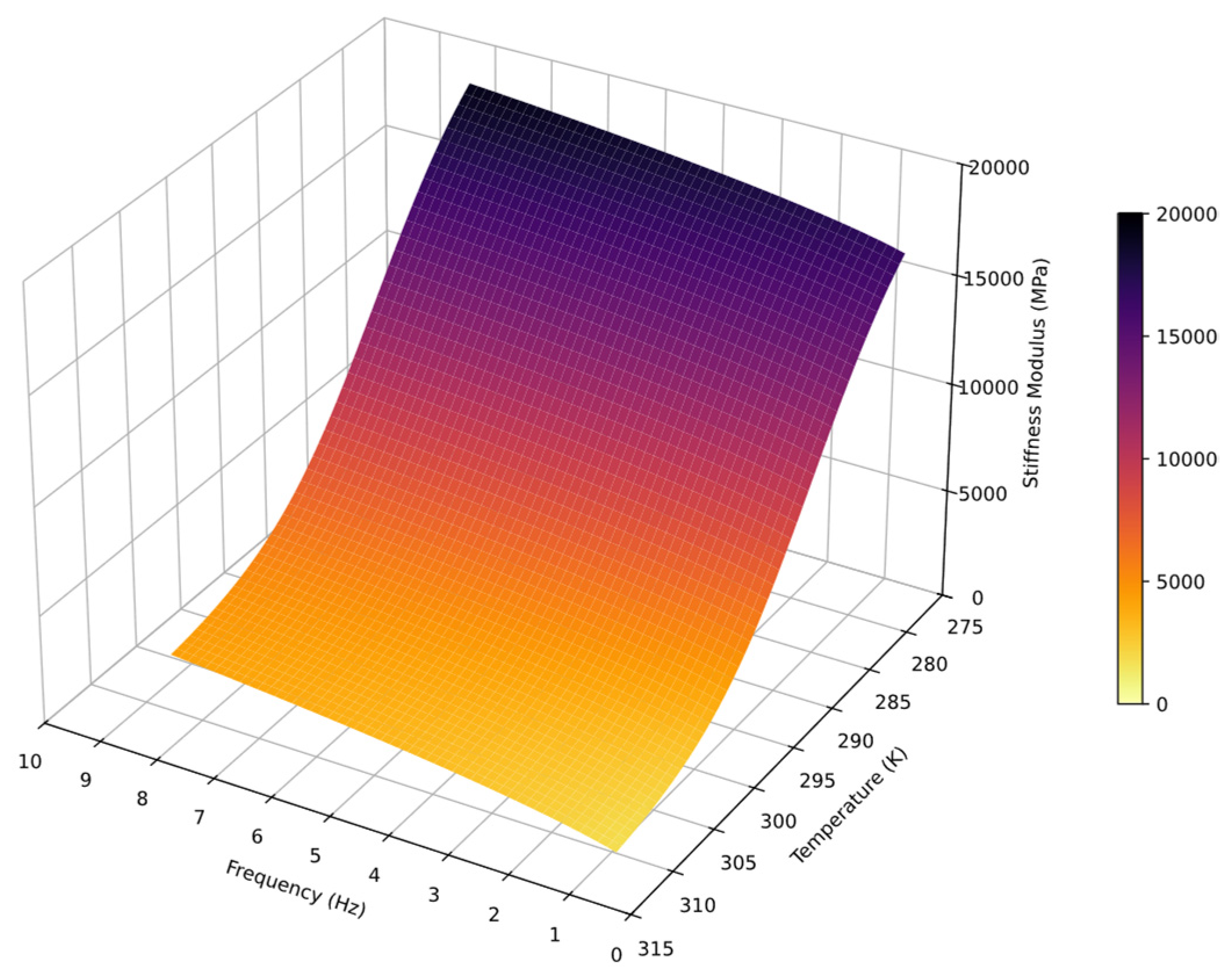
The concept of master curves is arguably widely used due to its straightforward graphical interpretation. In this regard, the TSI model can be used as a basis to evolve from the classical master curves to a new envelope designated as the Stiffness Prediction Surface (SPS). The SPS is a new concept (herein introduced) that can be defined as “a single continuous hypersurface that represents the whole set of possible stiffness moduli within the range of experimentally assessed loading conditions”. Thus, this qualitative description complements the quantitative formulation of the TSI model, i.e., Equation (22). Figure 6 shows an example of the SPS for the HMA-0 design. As shown in this graph, the advantages of the SPS over the traditional master curve concept can be summarized in two key points: (i) a continuous “degradation” of stiffness can be observed, which gives additional insight into the relative influence of loading conditions (i.e., frequency and temperature) on the stiffness across the temperature–frequency space; and (ii) the SPS obtained from the TSI model yields a smooth surface that simplifies the interpolation between points measured in the laboratory, which could be used to (effortlessly) identify possible anomalies in the experimental recordings.

5.4. Contributions to the Literature and Practical Applications

The proposed master curve formulation offers a valuable contribution to both the academic literature and the field of pavement engineering. Its integration into practice may support stakeholders such as engineers, designers, and public agencies in representing the mechanical behaviour of asphalt mixtures more accurately under realistic loading and environmental conditions. The TSI model introduced in this study serves as a predictive tool for assessing the stiffness evolution of asphalt mixtures in response to temperature variations, a critical factor for evaluating pavement durability and optimizing structural design. One important application involves the design of perpetual pavements, which are intended to maintain structural integrity over 5–6 decades without major interventions [82,83]. Ensuring long-term performance in such systems requires the control of strain levels within endurance limits, which in turn depends on reliable stiffness modulus values [84,85]. Given that stiffness is temperature-dependent and will be affected by long-term climate trends [86,87], the TSI model provides a framework for simulating these variations and informing annual performance assessments based on thermal conditions. A second relevant scenario concerns construction in arid regions, where extreme diurnal temperature shifts can impose significant thermal stresses on pavement materials [88,89]. In such environments, traditional design approaches based on constant in-service temperature assumptions are insufficient. Instead, the TSI model enables the estimation of stiffness moduli throughout the day, offering a more realistic basis for evaluating structural capacity under cyclic thermal loading. These examples illustrate the model’s potential to enhance design accuracy and performance prediction. Nevertheless, further applied research is needed to validate and refine its use in diverse contexts.
Another important aspect for the adoption in practice of the proposed TSI model is its future inclusion into pavement design software. Currently, leading design platforms (such as AASHTOWare Pavement ME Design, DARWin-ME, FlexPAVE, IMoDin, and VEROAD) rely on the traditional approach, which combines a conventional master curve model with shift factor formulations. The TSI model is ready to be implemented in this kind of software because it is openly published, allowing any user or developer to access, adapt, and integrate it freely. Furthermore, its algebraic formulation is equivalent to that of conventional master curve models, meaning it does not impose significantly greater demands in terms of computational time or memory during calibration. In addition, the TSI model offers superior numerical/computational stability compared to traditional models, which supports seamless and reliable integration into existing software environments used for pavement design.

5.5. Research Limitations

Although the TSI model effectively addresses key limitations of conventional master curve formulations, its implementation requires the calibration of three additional fitting parameters. The preceding increases the total number of parameters to seven, thereby raising the minimum experimental data requirements. Many optimization techniques, whether deterministic or stochastic, necessitate at least as many data points as there are fitting parameters to ensure reliable convergence and accurate solutions [90,91,92]. As a result, whereas traditional master curves (e.g., GS, CS, SLS, and uniaxial models) can be calibrated with four laboratory tests, the TSI model demands (at least) seven experimental measurements. This requirement poses a practical constraint, particularly in situations where material testing is limited by cost, time, or equipment availability, potentially restricting the broader application of the model in routine engineering practice.
On the other hand, it is important to acknowledge a limitation of the addressed case study, where the stiffness modulus was evaluated under only 20 loading conditions, combining 5 frequencies (0.5, 1, 2, 4, and 8 Hz) with 4 temperatures (5, 10, 20, and 40 °C). For future research, it is essential to assess the performance of the proposed TSI model under a broader range of loading conditions, including much lower and higher frequencies, extremely low temperatures (including sub-zero conditions), and very high temperatures (e.g., 50–70 °C), where asphalt mixtures begin to exhibit more liquid-like behaviour.

5.6. Future Research Lines

The findings presented in this investigation should be regarded as preliminary, offering a foundation for further refinement and extension. One promising direction is to validate the model’s applicability to specialized asphalt mixtures, such as those engineered for high-inertia pavements or rapid drainage systems. Another avenue involves assessing its performance under constrained experimental conditions, for example, when calibration is based solely on data from extreme frequencies or low temperatures. In order to address practical limitations in experimental resources, the development of optimization algorithms driven by artificial intelligence (e.g., genetic algorithms) could enable robust calibration using a reduced number of test points [93,94]. Lastly, incorporating predictive elements related to asphalt aging into the TSI model presents a valuable opportunity. This could be achieved by introducing additional sigmoidal components with parameters linked to rheological indices that evolve with aging duration and severity, following recent advances in the literature [95,96]. Thus, these research directions would not only enhance the versatility of the TSI model but also contribute to a more comprehensive understanding of asphalt behaviour under varying environmental and mechanical conditions.

6. Summary and Conclusions

This investigation focuses on developing the TSI model, a thermodynamically based master curve with explicitly incorporated temperature dependence for asphalt mixtures. Thus, this manuscript covers the mathematical formulation of the TSI model and its further implementation in a case study that comprises four HMAs and four WMAs. In this case study, the stiffness modulus was obtained for 20 different loading conditions, i.e., the combination of 5 frequencies (0.5, 1, 2, 4, and 8 Hz) and 4 temperatures (5, 10, 20, and 40 °C). Additionally, the proposed TSI model was compared against the traditional approach for predicting the stiffness modulus of asphalt mixtures. In this regard, the following conclusions can be drawn from this research effort:
  • The development of the TSI model from thermodynamics-based principles (such as Eyring’s rate theory and activation free energy) and the TTSP proves that it is possible to accurately simulate the stiffness modulus of asphalt mixtures by explicitly accounting for both temperature and frequency as state variables. Specifically, the TSI model improves upon the traditional GS model by introducing three thermal-related fitting parameters (i.e., ψ , χ , and ϕ ), which enable a more precise and physically grounded characterization of the temperature-dependent behaviour of asphalt mixtures.
  • The fitting parameters ψ and χ capture the influences of the activation entropy and activation enthalpy, respectively. Meanwhile, ϕ introduces transition rate control and asymmetry into the model, enabling a more realistic representation of thermo-rheological behaviour in asphalt mixtures with complex mechanical responses; the preceding is particularly useful to account for effects caused by polymer modification, aging, and additive incorporation.
  • For the addressed case study, the TSI model delivers highly accurate predictions of the asphalt mixture’s stiffness modulus, with R2 scores above 0.98 and MAPE values below 8.5%. In particular, the TSI model demonstrated exceptional computational stability, with a non-convergence rate of just 0.04% across 8000 runs, making it 4 to 45 times more stable than traditional master curve models such as GS, uniaxial, CS, and SLG. This level of stability is remarkably high, especially considering that the calibration was performed over a narrow frequency spectrum (i.e., from 0.5 to 8 Hz), a condition under which conventional models often struggle. This superior performance is attributed to its dual-sigmoidal structure and foundation on the (also stable) GS model, allowing for localized fitting and improved robustness during calibration.
  • A benchmarking analysis confirmed that the proposed TSI model offers greater reliability than the traditional approach, which builds a master curve at a reference temperature and further relies on shift factors (e.g., Arrhenius or WLF formulations) to estimate stiffness at target temperatures. While the traditional method produced larger prediction errors (e.g., exceeding 200% at 40 °C), the TSI model maintained consistent accuracy across all loading conditions, with generally lower MAPE values and higher R2 scores, revealing its superior robustness and predictive capability.
  • The TSI model lays the foundation for advancing beyond the traditional master curve concept toward a new notion introduced in this study, i.e., the SPS. Basically, the SPS can be defined as a continuous hypersurface representing the full range of possible stiffness modulus values within the boundaries of the experimentally assessed loading conditions.

Author Contributions

Conceptualization, D.C. and R.P.-M.; methodology, R.P.-N. and G.M.-A.; software, D.C. and R.P.-M.; validation, R.P.-N. and G.M.-A.; formal analysis, O.G.-B. and R.P.-M.; investigation, D.C., O.G.-B., and R.P.-M.; resources, G.M.-A.; data curation, D.C. and R.P.-M.; writing—original draft preparation, D.C., O.G.-B., and R.P.-M.; writing—review and editing, R.P.-N. and G.M.-A.; visualization, D.C., O.G.-B., and R.P.-M.; supervision, R.P.-N. and G.M.-A.; project administration, G.M.-A.; funding acquisition, G.M.-A. All authors have read and agreed to the published version of the manuscript.

Funding

The authors thank the Department of Science, Technology, and Innovation (COLCIENCIAS) for supporting this investigation through the “Research Project 745/2016, Contract 037-2017, No. 1215-745-59105”.

Data Availability Statement

Some or all data, models, or code that support the findings of this study are available from the corresponding author upon reasonable request.

Conflicts of Interest

The authors declare that they have no known competing financial interests or personal relationships that could have appeared to influence the work reported in this paper.

References

  1. Al-Adham, K.; Baig, M.G.; Wahhab, H.A.A. Prediction of Dynamic Modulus for Elastomer-Modified Asphalt Concrete Mixes at Desert Environment. Arab. J. Sci. Eng. 2019, 44, 4141–4149. [Google Scholar] [CrossRef]
  2. Brondani, C.; Menezes Vestena, P.; Faccin, C.; Lisboa Schuster, S.; Pivoto Specht, L.; da Silva Pereira, D. Moisture Susceptibility of Asphalt Mixtures: 2S2P1D Rheological Model Approach and New Index Based on Dynamic Modulus Master Curve Changes. Constr. Build. Mater. 2022, 331, 127316. [Google Scholar] [CrossRef]
  3. Primusz, P.; Tóth, C. Use of the Modified Ramberg-Osgood Material Model to Predict Dynamic Modulus Master Curves of Asphalt Mixtures. Materials 2023, 16, 531. [Google Scholar] [CrossRef] [PubMed]
  4. Ling, M.; Luo, X.; Gu, F.; Lytton, R.L. Time-Temperature-Aging-Depth Shift Functions for Dynamic Modulus Master Curves of Asphalt Mixtures. Constr. Build. Mater. 2017, 157, 943–951. [Google Scholar] [CrossRef]
  5. Fan, X.; Lv, S.; Ge, D.; Liu, C.; Peng, X.; Ju, Z. Time-Temperature Equivalence and Unified Characterization of Asphalt Mixture Fatigue Properties. Constr. Build. Mater. 2022, 359, 129118. [Google Scholar] [CrossRef]
  6. Naderi, K.; Nejad, F.M.; Khodaii, A. Time-Temperature-Age Superposition Validation for Linear Viscoelastic Properties of Bituminous Materials. J. Mater. Civ. Eng. 2018, 30, 04017292. [Google Scholar] [CrossRef]
  7. Qin, X.; Ma, L.; Wang, H. Comparison Analysis of Dynamic Modulus of Asphalt Mixture: Indirect Tension and Uniaxial Compression Test. Transp. A Transp. Sci. 2019, 15, 165–178. [Google Scholar] [CrossRef]
  8. Lee, K.; Pape, S.; Castorena, C.; Kim, Y.R. Evaluation of Small Specimen Geometries for Asphalt Mixture Performance Testing and Pavement Performance Prediction. Transp. Res. Rec. 2017, 2631, 74–82. [Google Scholar] [CrossRef]
  9. Jing, R.; Varveri, A.; Liu, X.; Scarpas, A.; Erkens, S. Differences in the Ageing Behavior of Asphalt Pavements with Porous and Stone Mastic Asphalt Mixtures. Transp. Res. Rec. 2021, 2675, 1138–1149. [Google Scholar] [CrossRef]
  10. Zhao, Y.; Bai, L.; Liu, H. Implementation of a Triaxial Dynamic Modulus Master Curve in Finite-Element Modeling of Asphalt Pavements. J. Mater. Civ. Eng. 2014, 26, 491–498. [Google Scholar] [CrossRef]
  11. Zou, G.; Zhang, X.; Xu, J.; Chi, F. Morphology of Asphalt Mixture Rheological Master Curves. J. Mater. Civ. Eng. 2010, 22, 806–810. [Google Scholar] [CrossRef]
  12. Podolsky, J.H.; Williams, R.C.; Cochran, E. Effect of Corn and Soybean Oil Derived Additives on Polymer-Modified HMA and WMA Master Curve Construction and Dynamic Modulus Performance. Int. J. Pavement Res. Technol. 2018, 11, 541–552. [Google Scholar] [CrossRef]
  13. Gu, L.; Chen, L.; Zhang, W.; Ma, H.; Ma, T. Mesostructural Modeling of Dynamic Modulus and Phase Angle Master Curves of Rubber Modified Asphalt Mixture. Materials 2019, 12, 1667. [Google Scholar] [CrossRef] [PubMed]
  14. Wang, Z.; Lu, W.; Liu, K.; Lv, S.; Peng, X.; Yang, S.; Ding, S. Research on Failure Strength Master Curve and Fatigue Performance of Asphalt Mixture Containing High-Proportion Reclaimed Asphalt Pavement. Constr. Build. Mater. 2023, 370, 130537. [Google Scholar] [CrossRef]
  15. Xi, L.; Luo, R.; Ma, Q.; Tu, C.; Shah, Y.I. An Improved Method to Establish Continuous Relaxation Spectrum of Asphalt Materials. Constr. Build. Mater. 2022, 354, 129182. [Google Scholar] [CrossRef]
  16. Bi, Y.; Wei, R.; Li, R.; Zhang, J.; Pei, J. Evaluation of Rheological Master Curves of Asphalt Mastics and Asphalt-Filler Interaction Indices. Constr. Build. Mater. 2020, 265, 120046. [Google Scholar] [CrossRef]
  17. Chen, H.; Barbieri, D.M.; Zhang, X.; Hoff, I. Reliability of Calculation of Dynamic Modulus for Asphalt Mixtures Using Different Master Curve Models and Shift Factor Equations. Materials 2022, 15, 4325. [Google Scholar] [CrossRef]
  18. Wang, D.; Cannone Falchetto, A.; Riccardi, C.; Wistuba, M.P. Investigation on the Low Temperature Properties of Asphalt Binder: Glass Transition Temperature and Modulus Shift Factor. Constr. Build. Mater. 2020, 245, 118351. [Google Scholar] [CrossRef]
  19. Lorenz, B.; Pyckhout-Hintzen, W.; Persson, B.N.J. Master Curve of Viscoelastic Solid: Using Causality to Determine the Optimal Shifting Procedure, and to Test the Accuracy of Measured Data. Polymer 2014, 55, 565–571. [Google Scholar] [CrossRef]
  20. Chen, M.; Javilla, B.; Hong, W.; Pan, C.; Riara, M.; Mo, L.; Guo, M. Rheological and Interaction Analysis of Asphalt Binder, Mastic and Mortar. Materials 2019, 12, 128. [Google Scholar] [CrossRef]
  21. Su, N.; Xiao, F.; Wang, J.; Amirkhanian, S. Precision Analysis of Sigmoidal Master Curve Model for Dynamic Modulus of Asphalt Mixtures. J. Mater. Civ. Eng. 2018, 30, 04018290. [Google Scholar] [CrossRef]
  22. Calderon, E.; Leiva, P.; Loria, L.; Clark, D. LM-PI-UMP-017-R3: Herramienta de Calculo de La Curva Maestra de Modulo Dinamico-IModin 2.0. LanammeUCR. 2019, pp. 1–29. Available online: https://www.lanamme.ucr.ac.cr/repositorio/bitstream/handle/50625112500/194/LM-PI-UMP-017.pdf (accessed on 20 August 2025).
  23. Zhao, Y.; Tang, J.; Liu, H. Construction of Triaxial Dynamic Modulus Master Curve for Asphalt Mixtures. Constr. Build. Mater. 2012, 37, 21–26. [Google Scholar] [CrossRef]
  24. Pszczola, M.; Jaczewski, M.; Szydlowski, C. Assessment of Thermal Stresses in Asphalt Mixtures at Low Temperatures Using the Tensile Creep Test and the Bending Beam Creep Test. Appl. Sci. 2019, 9, 846. [Google Scholar] [CrossRef]
  25. Tabatabaee, H.; Velasquez, R.; Bahia, H. Modeling Thermal Stress in Asphalt Mixtures Undergoing Glass Transition and Physical Hardening. Transp. Res. Rec. 2012, 2296, 106–114. [Google Scholar] [CrossRef]
  26. Tan, G.; Wang, W.; Cheng, Y.; Wang, Y.; Zhu, Z. Master Curve Establishment and Complex Modulus Evaluation of SBS-Modified Asphalt Mixture Reinforced with Basalt Fiber Based on Generalized Sigmoidal Model. Polymers 2020, 12, 1586. [Google Scholar] [CrossRef]
  27. Liu, H.; Luo, R. Development of Master Curve Models Complying with Linear Viscoelastic Theory for Complex Moduli of Asphalt Mixtures with Improved Accuracy. Constr. Build. Mater. 2017, 152, 259–268. [Google Scholar] [CrossRef]
  28. Li, J.; Xiao, F.; Amirkhanian, S.N.; Xu, O. Dynamic and Rutting Characteristics of Recycled Asphalt Mixtures Containing Natural Sand and Anti-Stripping Agents. J. Clean. Prod. 2021, 280, 124365. [Google Scholar] [CrossRef]
  29. Bayane, B.M.; Yang, E.; Yanjun, Q. Dynamic Modulus Master Curve Construction Using Christensen-Anderson-Marasteanu (CAM) Model. Int. J. Eng. Res. Appl. 2017, 7, 53–63. [Google Scholar] [CrossRef]
  30. Zhao, Y.; Chen, P.; Cao, D. Extension of Modified Havriliak-Negami Model to Characterize Linear Viscoelastic Properties of Asphalt Binders. J. Mater. Civ. Eng. 2016, 28, 04015195. [Google Scholar] [CrossRef]
  31. Vestena, P.M.; Schuster, S.L.; de Almeida, P.O.B., Jr.; Faccin, C.; Specht, L.P.; da Silva Pereira, D. Dynamic Modulus Master Curve Construction of Asphalt Mixtures: Error Analysis in Different Models and Field Scenarios. Constr. Build. Mater. 2021, 301, 124343. [Google Scholar] [CrossRef]
  32. Xiao, X.; Wang, J.; Wang, T.; Amirkhanian, S.N.; Xiao, F. Linear Visco-Elasticity of Asphalt in View of Proportion and Polarity of SARA Fractions. Fuel 2024, 363, 130955. [Google Scholar] [CrossRef]
  33. Graziani, A.; Cardone, F.; Virgili, A. Characterization of the Three-Dimensional Linear Viscoelastic Behavior of Asphalt Concrete Mixtures. Constr. Build. Mater. 2016, 105, 356–364. [Google Scholar] [CrossRef]
  34. He, W.; Zhao, Z.; Zhang, Z.; Xiao, F. Modification and Application of the Arrhenius Equation Based on Activated Energy Methods from Various Asphalt Binders. J. Mater. Civ. Eng. 2024, 36, 04024123. [Google Scholar] [CrossRef]
  35. Tian, W.; Hu, C. Arrhenius Model-Based Analysis of High-Temperature Properties and Temperature Sensitivity of SBS/CR Modified Asphalt. Constr. Build. Mater. 2025, 476, 141298. [Google Scholar] [CrossRef]
  36. Liang, B.; Chen, Y.; Lan, F.; Zheng, J. Evaluation of Rheological and Aging Behavior of Modified Asphalt Based on Activation Energy of Viscous Flow. Constr. Build. Mater. 2022, 321, 126347. [Google Scholar] [CrossRef]
  37. Williams, M.L.; Landel, R.F.; Ferry, J.D. The Temperature Dependence of Relaxation Mechanisms in Amorphous Polymers and Other Glass-Forming Liquids. J. Am. Chem. Soc. 1955, 77, 3701–3707. [Google Scholar] [CrossRef]
  38. McCrum, N.G.; Pogany, G.A. Time-Temperature Superposition in the α Region of an Epoxy Resin. J. Macromol. Sci. Part B 1970, 4, 109–125. [Google Scholar] [CrossRef]
  39. Alrashydah, E.I.; Abo-Qudais, S.A. Hot Mix Asphalt Time-Temperature Shifting and Fitting Techniques: A Comparative Study. Constr. Build. Mater. 2017, 146, 514–523. [Google Scholar] [CrossRef]
  40. Pellinen, T.K.; Witczak, M.W.; Bonaquist, R.F. Asphalt Mix Master Curve Construction Using Sigmoidal Fitting Function with Non-Linear Least Squares Optimization. In Advances in Materials Characterization and Modeling of Pavement Systems; American Society of Civil Engineers: Reston, VA, USA, 2003; pp. 83–101. [Google Scholar]
  41. Fesko, D.G.; Tschoegl, N.W. Time-Temperature Superposition in Styrene/Butadiene/Styrene Block Copolymers. Int. J. Polym. Mater. 1974, 3, 51–79. [Google Scholar] [CrossRef]
  42. Qadir, A. Investigation of Glass Transition Temperature of Asphalt Concrete. J. Test. Eval. 2017, 45, 1680–1690. [Google Scholar] [CrossRef]
  43. Kang, Y.; Zhou, D.; Wu, Q.; Liang, R.; Shangguan, S.; Liao, Z.; Wei, N. Molecular Dynamics Study on the Glass Forming Process of Asphalt. Constr. Build. Mater. 2019, 214, 430–440. [Google Scholar] [CrossRef]
  44. Yang, G.; Wang, X.; Zhou, X.; Wang, Y. Experimental Study on the Phase Transition Characteristics of Asphalt Mixture for Stress Absorbing Membrane Interlayer. Materials 2020, 13, 474. [Google Scholar] [CrossRef] [PubMed]
  45. Liu, J.; Sun, Y.; Wang, W.; Chen, J. Using the Viscoelastic Parameters to Estimate the Glass Transition Temperature of Asphalt Binders. Constr. Build. Mater. 2017, 153, 908–917. [Google Scholar] [CrossRef]
  46. Zhang, Q.; Zhao, J.; Guo, S. Asphalt Rheological Properties Transformation from Frequency Domain to Temperature Domain Based on WLF Equation. Int. J. Pavement Res. Technol. 2023, 16, 167–175. [Google Scholar] [CrossRef]
  47. Ashter, S.A. Mechanics of Materials. Thermoforming of Single and Multilayer Laminates; Elsevier: Amsterdam, The Netherlands, 2014; pp. 123–145. [Google Scholar]
  48. Duque, J.; Martinez-Arguelles, G.; Nuñez, Y.; Peñabaena-Niebles, R.; Polo-Mendoza, R. Designing Climate Change (CC)-Resilient Asphalt Pavement Structures: A Comprehensive Literature Review on Adaptation Measures and Advanced Soil Constitutive Models. Results Eng. 2024, 24, 103648. [Google Scholar] [CrossRef]
  49. Lali, F.A.; Singh, R.R.; Haider, S.W.; Kutay, M.E.; Chatti, K.; Schenkel, J.P. Characterizing the Damaged Dynamic Modulus Master Curves of Existing Hot Mix Asphalt (HMA) Layers for Rehabilitation Design. Constr. Build. Mater. 2025, 483, 141808. [Google Scholar] [CrossRef]
  50. Forough, S.A.; Nejad, F.M.; Khodaii, A. Comparing Various Fitting Models to Construct the Tensile Relaxation Modulus Master Curve of Asphalt Mixes. Int. J. Pavement Eng. 2016, 17, 314–330. [Google Scholar] [CrossRef]
  51. Hou, S.; Deng, Y.; Jin, R.; Shi, X.; Luo, X. Relationships between Physical, Mechanical and Acoustic Properties of Asphalt Mixtures Using Ultrasonic Testing. Buildings 2022, 12, 306. [Google Scholar] [CrossRef]
  52. Zhang, R.; Sias, J.E.; Dave, E.V. Using Mix Design Information for Modelling of Fundamental Viscoelasticity of Asphalt Mixtures. Constr. Build. Mater. 2022, 329, 127029. [Google Scholar] [CrossRef]
  53. Oshone, M.; Sias, J.E.; Dave, E.V.; Martin, A.E.; Kaseer, F.; Rahbar-Rastegar, R. Exploring Master Curve Parameters to Distinguish between Mixture Variables. Road Mater. Pavement Des. 2019, 20, S812–S826. [Google Scholar] [CrossRef]
  54. Nitta, K. On a Thermodynamic Foundation of Eyring Rate Theory for Plastic Deformation of Polymer Solids. Philos. Mag. Lett. 2023, 103, 2186190. [Google Scholar] [CrossRef]
  55. Hao, T. The Empty World–A View from the Free Volume Concept and Eyring’s Rate Process Theory. Phys. Chem. Chem. Phys. 2024, 26, 26156–26191. [Google Scholar] [CrossRef]
  56. American Chemical Society. Eyring Outlines Absolute Rate Theory for Chemical Reactions. Chem. Eng. News Arch. 1951, 29, 1100–1101. [Google Scholar] [CrossRef]
  57. Urry, D.W. Henry Eyring (1901–1981): A 20th Century Physical Chemist and His Models. Math. Model. 1982, 3, 503–522. [Google Scholar] [CrossRef]
  58. Zhu, C.; Yang, F.; Liu, X.; Afzal, W.; He, M. Viscosity of Oxygenated Fuel: A Model Based on Eyring’s Absolute Rate Theory. Fuel 2019, 241, 218–226. [Google Scholar] [CrossRef]
  59. Hu, Y.F.; Lee, H. Prediction of Viscosity of Mixed Electrolyte Solutions Based on the Eyring’s Absolute Rate Theory and the Semi-Ideal Hydration Model. Electrochim. Acta 2003, 48, 1789–1796. [Google Scholar] [CrossRef]
  60. He, M.; Zhu, C.; Liu, X. Estimating the Viscosity of Ionic Liquid at High Pressure Using Eyring’s Absolute Rate Theory. Fluid Phase Equilib. 2018, 458, 170–176. [Google Scholar] [CrossRef]
  61. Hernández, A.; Khosharay, S. Investigation on the Surface Tension and Viscosity of (Dimethylsulfoxide + Alcohol) Mixtures by Using Gradient Theory and Eyring’s Rate Theory. Int. J. Thermophys. 2020, 41, 150. [Google Scholar] [CrossRef]
  62. Eyring, H.; Urry, D.W. The Theory of Absolute Reaction Rates in Solution. Berichte Der Bunsenges. Für Phys. Chem. 1963, 67, 731–740. [Google Scholar] [CrossRef]
  63. Li, S. Numerical Investigation on Viscoelastic Response of Asphalt Mixture under Tire Braking Slip. Case Stud. Constr. Mater. 2023, 18, e02009. [Google Scholar] [CrossRef]
  64. Zhang, J.; Faruk, A.N.M.; Karki, P.; Holleran, I.; Hu, X.; Walubita, L.F. Relating Asphalt Binder Elastic Recovery Properties to HMA Cracking and Fracture Properties. Constr. Build. Mater. 2016, 121, 236–245. [Google Scholar] [CrossRef]
  65. Bai, T.; Cheng, Z.; Hu, X.; Fuentes, L.; Walubita, L.F. Viscoelastic Modelling of an Asphalt Pavement Based on Actual Tire-Pavement Contact Pressure. Road Mater. Pavement Des. 2021, 22, 2458–2477. [Google Scholar] [CrossRef]
  66. Modi, S.H.; Orešković, M.; Dave, E.V.; Sias, J.E. Application of Time-Temperature Superposition Principle for Cracking Characterization of Asphalt Mixtures Using Semi-Circular Bend Test. Constr. Build. Mater. 2024, 443, 137647. [Google Scholar] [CrossRef]
  67. Phan, T.N.; Nguyen, N.H.; Do, T.T.; Nguyen, H.T.T.; Nguyen, M.L. Verification of Time-Temperature Superposition Principle for Viscoplastic Strains of Asphalt Mixtures Obtained from Creep-Recovery Tests in the Low-Strain Regime. Road Mater. Pavement Des. 2025, 26, 958–995. [Google Scholar] [CrossRef]
  68. Bradai, M.A.; Tapsoba, N.; Sauzéat, C.; Di Benedetto, H.; Neji, J. Validation of the Time-Temperature Superposition Principle (TTSP) in the Non-Linear Domain for Bituminous Mixtures with Reclaimed Asphalt Pavement (40% RAP). In RILEM International Symposium on Bituminous Materials; Springer: Berlin/Heidelberg, Germany, 2022; pp. 1925–1931. [Google Scholar]
  69. Zhao, Y.; Richard Kim, Y. Time–Temperature Superposition for Asphalt Mixtures with Growing Damage and Permanent Deformation in Compression. Transp. Res. Rec. J. Transp. Res. Board 2003, 1832, 161–172. [Google Scholar] [CrossRef]
  70. Covilla-Varela, E.; Turbay, E.; Polo-Mendoza, R.; Martínez-Arguelles, G.; Cantero-Durango, J. Recycled Concrete Aggregates (RCA)-Based Asphalt Mixtures: A Performance-Related Evaluation with Sustainability-Criteria Verification. Constr. Build. Mater. 2023, 403, 133203. [Google Scholar] [CrossRef]
  71. Martinez-Arguelles, G.; Dugarte, M.; Fuentes, L.; Sanchez, E.; Rondon, H.; Pacheco, C.; Yepes, J.; Lagares, R. Characterization of Recycled Concrete Aggregate as Potential Replacement of Natural Aggregate in Asphalt Pavement. In IOP Conference Series: Materials Science and Engineering; IOP Publishing: Bristol, UK, 2019; Volume 471, p. 102045. [Google Scholar] [CrossRef]
  72. Le, T.M.; Fatahi, B.; Khabbaz, H.; Sun, W. Numerical Optimization Applying Trust-Region Reflective Least Squares Algorithm with Constraints to Optimize the Non-Linear Creep Parameters of Soft Soil. Appl. Math. Model. 2017, 41, 236–256. [Google Scholar] [CrossRef]
  73. Rahman, A.A.; Wang, B.; Yan, J.; Wang, H.; Jin, T.; Gan, Z. Developed Empirical Correlation for Self-Pressurization in Multi-Configuration Non-Venting Liquid Hydrogen Tanks Using Trust-Region Reflective Algorithm. Int. J. Hydrogen Energy 2025, 142, 122–129. [Google Scholar] [CrossRef]
  74. Weiping, W.; Hongchun, W.; Haofeng, Z.; Xiong, X. A Pn-Wave Spectral Inversion Technique Based on Trust Region Reflective Algorithm. J. Appl. Geophy. 2024, 230, 105525. [Google Scholar] [CrossRef]
  75. Shireman, E.; Steinley, D.; Brusco, M.J. Examining the Effect of Initialization Strategies on the Performance of Gaussian Mixture Modeling. Behav. Res. Methods 2017, 49, 282–293. [Google Scholar] [CrossRef]
  76. Karlis, D.; Xekalaki, E. Choosing Initial Values for the EM Algorithm for Finite Mixtures. Comput. Stat. Data Anal. 2003, 41, 577–590. [Google Scholar] [CrossRef]
  77. Singh, R.R.; Lali, F.; Muslim, H.B.; Haider, S.W.; Dolan, K.D. Scaled Sensitivity of Pavement–Mechanistic-Empirical Transfer Function Coefficients for Flexible and Rigid Pavements. Transp. Res. Rec. J. Transp. Res. Board 2025, 2679, 630–640. [Google Scholar] [CrossRef]
  78. Scharmack, D.K. An Initial Value Method for Trajectory Optimization Problems. In Advances in Control Systems; Elsevier: Amsterdam, The Netherlands, 1967; pp. 51–132. [Google Scholar]
  79. Korošec, P.; Eftimov, T. Insights into Exploration and Exploitation Power of Optimization Algorithm Using DSCTool. Mathematics 2020, 8, 1474. [Google Scholar] [CrossRef]
  80. Biernacki, C.; Celeux, G.; Govaert, G. Choosing Starting Values for the EM Algorithm for Getting the Highest Likehood in Multivariate Gaussian Mixture Models. Comput. Stat. Data Anal. 2003, 41, 561–575. [Google Scholar] [CrossRef]
  81. Brugnano, L.; Trigiante, D. Convergence and Stability of Boundary Value Methods for Ordinary Differential Equations. J. Comput. Appl. Math. 1996, 66, 97–109. [Google Scholar] [CrossRef]
  82. Walubita, L.F.; Scullion, T.; Leidy, J.; Liu, W. Non-Destructive Testing Technologies: Application of the Ground Penetrating Radar (GPR) to Perpetual Pavements. Road Mater. Pavement Des. 2009, 10, 259–286. [Google Scholar] [CrossRef]
  83. Yang, Y.; Wei, J.; Lin, W.; Timm, D.; Huber, G. Binzhou Perpetual Pavement Test Road: Dynamic Response of Pavement under Very Heavy Loads. Road Mater. Pavement Des. ICAM 2009, 10, 151–165. [Google Scholar] [CrossRef]
  84. Mazumder, M.; Kim, H.; Lee, S.J. Perpetual Pavement: Future Pavement Network. J. Adv. Constr. Mater. 2015, 19, 35–49. [Google Scholar]
  85. El-Hakim, M.Y.; Tighe, S.L. Sustainability of Perpetual Pavement Designs: Canadian Perspective. Transp. Res. Rec. 2012, 2304, 10–16. [Google Scholar] [CrossRef]
  86. Halle, M.; Rukavina, T.; Domitrovic, J. Influence of Temperature on Asphalt Stiffness Modulus. In Proceedings of the 5th Eurasphalt & Eurobitume Congress, Istanbul, Turkey, 13–15 June 2012; pp. 1–12. [Google Scholar]
  87. Moghaddam, T.B.; Soltani, M.; Karim, M.R. Stiffness Modulus of Polyethylene Terephthalate Modified Asphalt Mixture: A Statistical Analysis of the Laboratory Testing Results. Mater. Des. 2015, 68, 88–96. [Google Scholar] [CrossRef]
  88. Radwan, M.M.; Mousa, A.; Zahran, E.M.M. Enhancing Pavement Sustainability: Prediction of the Pavement Condition Index in Arid Urban Climates Using the International Roughness Index. Sustainability 2024, 16, 3158. [Google Scholar] [CrossRef]
  89. Al-Abdul Wahhab, H.I.; Balghunaim, F.A. Asphalt Pavement Temperature Related to Arid Saudi Environment. J. Mater. Civ. Eng. 1994, 6, 8–14. [Google Scholar] [CrossRef]
  90. Emmerich, M.; Yang, K.; Deutz, A.; Wang, H.; Fonseca, C.M. A Multicriteria Generalization of Bayesian Global Optimization. In Advances in Stochastic and Deterministic Global Optimization; Pardalos, P.M., Zhigljavsky, A., Žilinskas, J., Eds.; Springer International Publishing: Berlin/Heidelberg, Germany, 2016; pp. 229–242. [Google Scholar]
  91. Li, C.; Grossmann, I.E. A Review of Stochastic Programming Methods for Optimization of Process Systems Under Uncertainty. Front. Chem. Eng. 2021, 2, 622241. [Google Scholar] [CrossRef]
  92. Arora, J.S.; Elwakeil, O.A.; Chahande, A.I.; Hsieh, C.C. Global Optimization Methods for Engineering Applications: A Review. Struct. Optim. 1995, 9, 137–159. [Google Scholar] [CrossRef]
  93. Kuptametee, C.; Michalopoulou, Z.H.; Aunsri, N. A Review of Efficient Applications of Genetic Algorithms to Improve Particle Filtering Optimization Problems. Measurement 2024, 224, 113952. [Google Scholar] [CrossRef]
  94. Neumann, A.; Hajji, A.; Rekik, M.; Pellerin, R. A Didactic Review On Genetic Algorithms For Industrial Planning And Scheduling Problems. IFAC-Pap. 2022, 55, 2593–2598. [Google Scholar] [CrossRef]
  95. Bi, Y.; Wu, S.; Pei, J.; Wen, Y.; Li, R. Correlation Analysis between Aging Behavior and Rheological Indices of Asphalt Binder. Constr. Build. Mater. 2020, 264, 120176. [Google Scholar] [CrossRef]
  96. Leite, L.F.M.; Osmari, P.H.; Aragão, F.T.S. Rheological Indexes for Asphalt Binders Considering Different Aging Conditions: Evaluation and Correlations with Performance. Constr. Build. Mater. 2022, 338, 127549. [Google Scholar] [CrossRef]
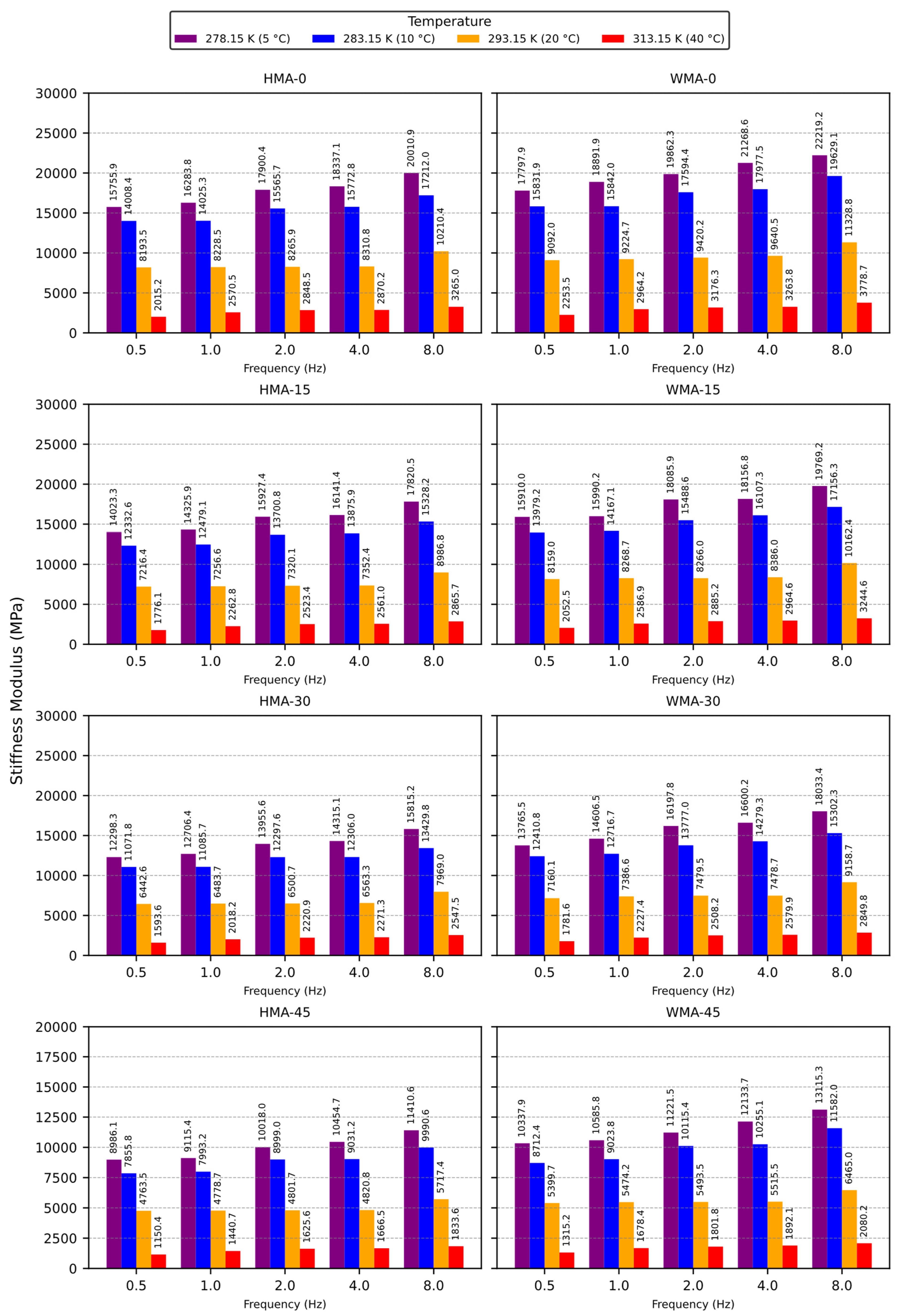
Figure 1. Laboratory-measured stiffness modulus of asphalt mixtures. Adapted from [70].
Infrastructures 10 00227 g001
Figure 2. Calibration of the proposed TSI model for the adopted case study.
Infrastructures 10 00227 g002
Figure 3. Correlations between fitting parameters and fundamental mixture characteristics.
Infrastructures 10 00227 g003
Figure 4. Master curves and experimental data for asphalt mixtures at 20 °C.
Infrastructures 10 00227 g004
Figure 5. Evolution of a T across target temperatures (i.e., 5, 10, and 40 °C) for each asphalt mixture.
Infrastructures 10 00227 g005
Figure 6. Example of SPS for the HMA-0 design.
Infrastructures 10 00227 g006
Table 2. Summary of shift factor models: equations, applicability, and limitations.
FormulationsBest
Temperature Range
Unreliable
Temperature Range
NotesReferences
Arrhenius
(Equation (6))
Low temperatures (glassy, below T g )At or above T g (rubbery)Assumes constant activation energy; suitable for glassy regime.[36,45]
WLF
(Equation (7))
Around and above T g Deep in glassy region (low T)Empirical constants; best near Tg.[17,18]
Kaelble:
l o g 10   a T = H 2.303 R T T r T · T r
Below and around T g (sub- T g )Far above T g   (highly rubbery region)More symmetric than WLF for sub-Tg; useful for describing both sides of Tg.[38,41]
Log-linear:
l o g 10   a T = A + B   ( T T r )
Wide temperature range (empirical)May lack physical basis at extremesSimple, flexible; used for practical fitting.[17]
Quadratic polynomial:
l o g 10   a T = a 0 +   a 1 T T r +   a 2 T T r 2
Wide temperature range (empirical)May overfit or lack physical meaningUseful for complex blends or modified asphalts.[17,39]
Table 3. Description of the asphalt mixtures considered in the case study. Adapted from [70].
Asphalt Mixtures a
HMA-0HMA-15HMA-30HMA-45WMA-0WMA-15WMA-30WMA-45
Gravimetric
composition
Fine NAs (%)47.8047.7047.5047.2547.8047.7547.6047.40
Coarse NAs (%)47.8040.5533.2525.9947.8040.5933.3226.07
Fine RCA (%)00000000
Coarse RCA (%)07.1614.2521.2607.1614.2821.33
Asphalt binder (%)4.404.605.005.504.404.504.805.20
Laboratory
characterization
Mixing temperature (°C)160.00160.00160.00160.00120.00120.00120.00120.00
Compaction temperature (°C)140.00140.00140.00140.00110.00110.00110.00110.00
Bulk density (kg/m3)2361.042351.372331.332322.252363.122333.982337.342317.63
VFA (%)69.6970.5468.6266.2770.5870.8469.4067.75
VMAs (%)14.3215.4115.7116.1014.6515.5015.8516.28
VTMs (%)4.344.544.935.434.314.524.855.25
Marshall flow value (mm)3.173.656.326.862.622.966.296.39
Marshall stability (kN)15.1314.5713.7412.8815.9315.2214.6013.89
Abbreviations: VFA—void filled with asphalt; VMAs—voids in mineral aggregate; VTMs—voids in the total mix. Notes: a—the number after the type of asphalt mixture indicates the coarse RCA content by total coarse aggregate weight.
Table 5. Convergence assessment for the adopted case study.
Asphalt MixturesNumber of Non-Convergent Runs
GS
Model
CS
Model
SLG
Model
Uniaxial
Model
TSI
Model
HMA-02221040
HMA-151121720
HMA-302192430
HMA-451172610
WMA-02132131
WMA-151191110
WMA-302221620
WMA-452141822
Total13138143183
Non-convergence (%)0.161.731.790.230.04
Traditional model/proposed model ratio (-)443456
Table 6. Fitting parameters of the GS model for asphalt mixtures at 20 °C.
Asphalt
Mixtures
Fitting Parameters
α β γ δ
HMA-03.907667−5.15.14.165368
HMA-153.853796−5.15.14.108047
HMA-303.804261−5.15.14.051765
HMA-453.673245−5.15.13.886199
WMA-03.961070−5.14.7402544.262092
WMA-153.908768−5.15.14.160014
WMA-303.858396−5.14.9838914.141897
WMA-453.731134−5.15.13.933298
Table 7. Calibrated empirical constants of the Arrhenius and WLF models.
Asphalt
Mixtures
Arrhenius
Model
WLF
Model
E a (J/mol) C 1 (-) C 2 (K)
HMA-0285,678.6611.9776.61
HMA-15288,933.5512.1076.54
HMA-30314,577.1613.1376.35
HMA-45513,774.3038.1068.76
WMA-0263,700.4214.3096.19
WMA-15293,735.4712.2976.51
WMA-30261,119.8314.0995.77
WMA-45513,693.1531.5470.89
Table 8. Shift factors for asphalt mixtures based on Arrhenius and WLF models.
Asphalt
Mixtures
Arrhenius ModelWLF Model
a T = 5 ° C a T = 10 ° C a T = 40 ° C a T = 5 ° C a T = 10 ° C a T = 40 ° C
HMA-05.5553 × 1026.2733 × 1015.6158 × 10−48.2233 × 1026.2733 × 1013.3214 × 10−3
HMA-155.9701 × 1026.5762 × 1015.1568 × 10−48.8825 × 1026.5762 × 1013.1187 × 10−3
HMA-301.0528 × 1039.5351 × 1012.6339 × 10−41.6254 × 1039.5351 × 1011.8790 × 10−3
HMA-458.6333 × 1041.7087 × 1031.4257 × 10−64.2690 × 10103.0466 × 1062.6027 × 10−9
WMA-03.4162 × 1024.5625 × 1019.9883 × 10−44.3861 × 1024.5625 × 1013.4546 × 10−3
WMA-156.6392 × 1027.0500 × 1014.5472 × 10−49.9453 × 1027.0500 × 1012.8353 × 10−3
WMA-303.2267 × 1024.3951 × 1011.0687 × 10−34.1402 × 1024.3951 × 1013.6779 × 10−3
WMA-458.6178 × 1041.7067 × 1031.4288 × 10−62.9222 × 1081.5148 × 1051.1457 × 10−7
Table 9. Prediction errors expressed as the MAPE (%) for the traditional approach across asphalt mixtures.
Asphalt
Mixtures
GS Model
(20 °C)
Arrhenius ModelWLF Model
5 °C10 °C40 °C5 °C10 °C40 °C
HMA-01.6616.526.35205.7716.526.35205.71
HMA-151.5617.436.48205.7617.426.47205.78
HMA-301.4717.826.86206.6217.826.86206.62
HMA-451.3722.4211.61213.2822.4211.60213.25
WMA-00.799.084.40204.819.104.40204.77
WMA-151.3317.226.83202.4717.226.81202.49
WMA-301.7811.933.69209.9911.953.69209.93
WMA-451.2024.7012.81214.4924.7312.82214.48
Table 10. R2 values for predictions from the GS model at the reference temperature.
Asphalt
Mixtures
GS Model
(20 °C)
HMA-00.9470
HMA-150.9522
HMA-300.9542
HMA-450.9458
WMA-00.9887
WMA-150.9621
WMA-300.9523
WMA-450.9514
Disclaimer/Publisher’s Note: The statements, opinions and data contained in all publications are solely those of the individual author(s) and contributor(s) and not of MDPI and/or the editor(s). MDPI and/or the editor(s) disclaim responsibility for any injury to people or property resulting from any ideas, methods, instructions or products referred to in the content.