Field-Test-Driven Sensitivity Analysis and Model Updating of Aging Railroad Bridge Structures Using Genetic Algorithm Optimization Approach

Abstract

Aging railroad bridges present complex challenges due to advancing deterioration and outdated design assumptions. This study develops a comprehensive analytical approach for assessing an aging steel truss railroad bridge through finite element (FE) modeling, sensitivity analysis, and model updating, supported by field testing. An initial FE model of the bridge was created based on original drawings and field observations. Field testing using a laser Doppler vibrometer captured the bridge’s dynamic response (vibrations and deflections) under regular train traffic. Key structural parameters (material properties, section properties, support conditions) were identified and varied in a sensitivity analysis to determine their influence on model outputs. A hybrid sensitivity analysis combining log-normal sampling and a genetic algorithm (GA) was employed to explore the parameter space and calibrate the model. The GA optimization tuned the FE model parameters to minimize discrepancies between simulated results and field measurements, focusing on vertical deflections and natural frequencies. The updated FE model showed significantly improved agreement with observed behavior; for example, vertical deflections under a representative train were matched within a few percent, and natural frequencies were accurately reproduced. This validated model provides a more reliable tool for predicting structural performance and fatigue life under various loading scenarios. The results demonstrate that integrating field data, sensitivity analysis, and model updating can greatly enhance the accuracy of structural assessments for aging railroad bridges, supporting more informed maintenance and management decisions.

1. Introduction

Aging infrastructure in the United States poses a significant concern as more railroad bridges exceed their operational lifespans [1,2]. When most railroad bridges were designed and built, load-carrying requirements, design codes, and material specifications differed significantly from today’s standards [3,4]. These bridges have operated for decades under intensifying and more frequent traffic from vehicles, along with unavoidable environmental exposure [5,6]. Consequently, these structures often face issues such as corrosion, fatigue cracking, and other forms of deterioration that compromise safety and serviceability, frequently exhibiting unusual behavior under standard service loads [7].

Addressing the complexity of aging bridges requires a multi-pronged approach involving detailed inspections, structural health monitoring (SHM), and rigorous analytical modeling [2,8]. Inspections remain the primary method for detecting visible signs of damage; however, they are often labor-intensive, subjective, and limited to accessible areas [9,10,11]. Furthermore, superficial examinations may not detect internal cracks, hidden corrosion, or incipient failures at riveted or welded connections [2,4]. To mitigate these limitations, SHM methods have gained prominence [12,13]. By employing sensors, including accelerometers and laser Doppler vibrometers, engineers can observe changes in dynamic behavior under ambient or controlled loading conditions [5,14]. Such measurements enable continuous or frequent evaluation of a structure’s condition, potentially identifying damage early, before it becomes visually apparent [15].

Despite its effectiveness, monitoring alone cannot fully elucidate the underlying mechanics of complex structural systems [16,17]. Localized damage may go undetected by a limited sensor network, or measured responses might be difficult to interpret without a baseline model [18,19]. Finite element (FE) models assume a crucial complementary role in analyzing aging bridges [13,20]. By discretizing the geometry into elements that approximate the actual behavior of steel truss members, deck systems, and connections, FE modeling provides a framework for simulating the structural response under various load scenarios [18,21]. Engineers can adjust boundary conditions, material properties, and connection details to capture the unique configuration of an older bridge, which may differ significantly from modern standardized designs [4,20]. With this computational representation in hand, it becomes possible to explore different what-if scenarios, such as increased live loads or localized damage, without conducting invasive or risky field tests [21,22].

However, the predictive accuracy of an FE model is not guaranteed at the outset [18,20]. Older bridges pose considerable uncertainty regarding existing material properties, residual capacity, and condition [4]. For instance, variations in steel composition, rivet strength, and section loss due to corrosion may all deviate from standardized assumptions [3,4,23]. Model updating, a process that systematically refines the FE model parameters to minimize discrepancies between measured and simulated responses, has proven to be an effective method for resolving these uncertainties [19,20]. By calibrating the model against field data, such as natural frequencies, mode shapes, and displacement responses, engineers can arrive at a high-fidelity representation of the aging bridge. This updated model is better suited for predicting the structure’s behavior under future load demands or environmental stressors [16,17]. Recent studies have extended model updating frameworks to a variety of aging structures, including concrete dams, bridge piers, and machine foundations, where degradation and dynamic behavior are similarly complex [24,25,26,27]. These applications show how parameter tuning, sensitivity-based updating, and field testing improve seismic safety evaluations and long-term resilience. Recent advances have integrated digital twin models with Bayesian updating for fatigue assessment and structural model calibration. Lai et al. [17] used SHM-informed Bayesian forecasting for life-cycle maintenance of fatigue-sensitive details, while Nhamage et al. [13] combined a fatigue analysis system with a BIM-based digital twin for real-time visualization and scenario simulation. Compared to these data-intensive approaches, the method in this study offers a more practical and computationally efficient alternative for bridges lacking continuous monitoring systems.

Within this broader context, sensitivity analysis is a powerful technique for identifying which parameters, such as Young’s modulus, cross-sectional area, or joint stiffness, exert the most significant influence on model outputs [18]. Because steel truss bridges often have complex load paths and connections, small changes in certain parameters can disproportionately affect global stiffness or dynamic characteristics [20,21]. By systematically varying these parameters within plausible ranges, one can highlight where knowledge gaps or uncertainties significantly impact the overall analysis [18]. In tandem with model updating, sensitivity analysis enables a more targeted data collection strategy: engineers can strategically place sensors to capture the most informative signals, and subsequent calibration can focus on the most consequential variables [17].

Integrating FE modeling, sensitivity analysis, and model updating lays the groundwork for proactive bridge management [6,16]. Rather than reacting to problems once they manifest visibly or result in service disruptions, agencies can continuously evaluate bridge conditions and adapt maintenance strategies as new information arises [5,6]. This approach fosters a dynamic process of structural assessment, where monitoring data feed into the model, the model guides inspection and monitoring strategies, and the calibration of the model refines the predictions of remaining service life or capacity [17,28]. Additionally, this workflow facilitates more accurate load ratings, ensuring that restrictions or rehabilitations are imposed only when genuinely necessary [6].

This paper outlines how FE modeling, sensitivity analysis, and model updating methods can be applied to an aging steel truss railroad bridge in the United States. The structure in question is both historically significant and essential for modern transportation needs, reflecting the broader national challenge of preserving heritage infrastructure under increasingly stringent performance demands. By conducting field tests to measure acceleration and displacement and systematically calibrating an FE model to align with these real-world measurements, this study demonstrates the efficacy of a comprehensive model updating approach in bridging the assessment. Sensitivity analysis identifies which parameters crucially affect the model’s fidelity, while iterative model updating refines predictions of the structure’s dynamic behavior and fatigue life [20]. Collectively, these tools help mitigate risks, optimize maintenance resources, and extend the operational lifespan of a critical railroad asset [6,16].

2. Bridge Description

The Cos Cob Bridge (Figure 1) is a long-span, open-deck truss railroad bridge located on the Mianus River in Greenwich, Connecticut. It is one of the old and historic bridges in Amtrak’s Northeast Corridor (NEC). The bridge was built in 1904 by the American Bridge Company and has been in operation for more than a century. The bridge is commonly used by passenger trains like Metro-North M8 (MTNR M8), Amtrak Regional, and Acela Express. The bridge has eleven simply supported spans resting on eleven stone piers and two abutments at the ends. Three of the sections are deck girder, seven are deck trusses, and one is a rolling lift bascule. The bridge has four tracks (Track 1, Track 2, Track 3, and Track 4), and each track sits on a separate parallel bridge. The track system on the bridge consists of steel rails mounted on timber sleepers (cross-ties), which are supported on the bridge deck. The rails are secured to the sleepers using conventional rail fastening systems to maintain proper alignment and load transfer. This study focuses on Track 4 of span 3 (Figure 2) because of its accessibility for field testing equipment, especially during periods of lowered water levels affected by tides.

Track 4 of span 3 has a span length of 37.2 m (122.1 ft) between pier centerlines. The four parallel track structures collectively span a total width of approximately 27.43 m (90 ft) across the river. All primary members of the bridge were fabricated from carbon steel meeting the ASTM A7 specification (common for early 20th-century steel bridges). The truss members have built-up cross-sections composed of steel plates forming I-shaped and C-shaped sections, connected by rivets. The truss members are connected with gusset plates, and lateral bracing systems are present at both the top and bottom levels of the truss. These lateral braces provide stability against transverse and vertical loads, respectively.

3. Methodology

This section presents the methodology adopted to evaluate the structural behavior of the bridge structure through a combination of field measurements and numerical modeling. The methodology includes field tests and data processing, FE modeling using ANSYS Mechanical, version 2025 R1, and sensitivity analysis for model updating using MATLAB R2022b and ANSYS Mechanical, Version 2025 R1. These components collectively support the comparison between measured responses and simulated results to assess and refine the accuracy of the analytical model.

3.1. Field Tests and Data Processing

A single-point laser Doppler vibrometer (LDV) was used to perform field testing on the bridge. An LDV is a non-contact optical instrument that emits a laser beam to measure surface vibration by detecting the Doppler shift in the reflected beam. Its output is typically a continuous analog voltage signal proportional to the velocity of the target’s motion along the laser line of sight [30]. In this study, the LDV was deployed to capture vertical vibration responses of the span during train passages. The LDV was mounted on a stable tripod placed at a safe distance from the bridge piers and bottom chords and aligned perpendicularly to the target surface to ensure a clear line of sight and minimize noise. Since the LDV operates without physical contact, it is inherently isolated from ground-transmitted vibrations, ensuring that only the structural response of the bridge is captured. Measurement locations were selected based on accessibility to capture representative dynamic responses. The LDV output was collected using a high-speed data acquisition system, with sampling conducted at 512 Hz to adequately capture both forced and free vibration signals during and after train passages.

Data were recorded in the time domain using a Polytec PSV^® data acquisition system and then processed in MATLAB^® [31], a widely used scientific computing platform. The LDV output, being a velocity-proportional voltage, required preprocessing to derive meaningful displacement and acceleration time histories. This involved applying a scaling factor (from the instrument calibration) to convert the voltage to physical velocity units and then integrating the velocity signal to obtain displacement. The data were also high-pass filtered to remove any DC bias (offset) in the signal, which is a common artifact in LDV measurements that can shift the mean away from zero [32]. The natural frequencies of the bridge were extracted from the free vibration portion of the signal recorded after the train had passed. The free vibration segment reflects the structure’s true dynamic characteristics without external excitation. After this conditioning, the resulting time histories of bridge deflection and acceleration were suitable for analysis in both time and frequency domains.

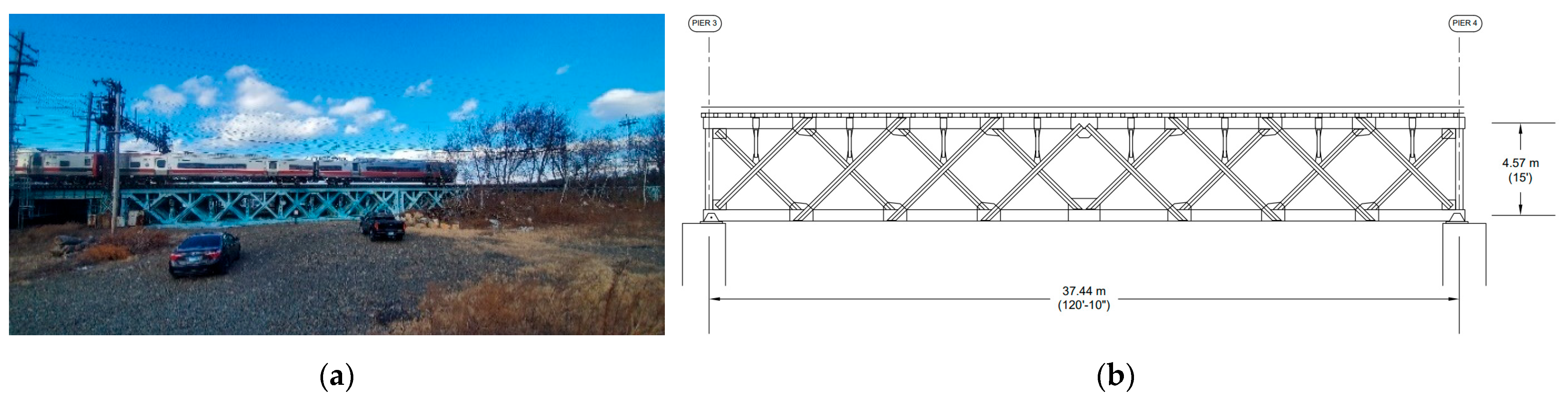
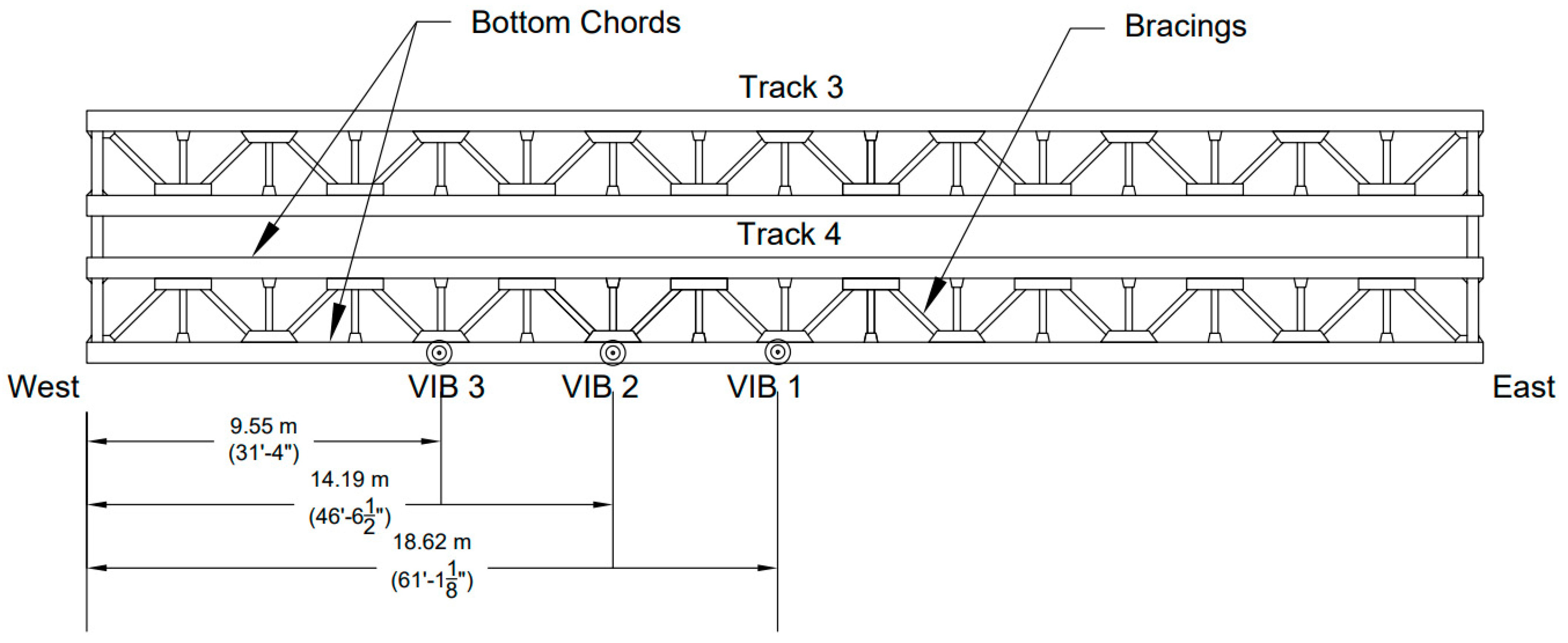
Field tests were conducted during normal service with trains of three types: Metro-North M8 commuter train, Amtrak’s Northeast Regional, and Amtrak’s Acela Express. The single-point LDV was mounted on a tripod beneath the span, aiming upward at the underside of the Track 4 structure (Figure 3), to measure vertical velocity during train crossings. The LDV was repositioned between tests to collect data at multiple points along the span. Specifically, bridge responses (velocity) were recorded at three different locations on span 3 (Track 4), designated as Vib 1, Vib 2, and Vib 3 (see Figure 4), where displacement results were desired. Multiple train passages were recorded at each sensor position to ensure reliable data under consistent operating conditions. All tests were performed with trains traveling from New York toward New Haven (west-to-east direction).

3.2. Finite Element Model

A three-dimensional finite element (FE) model of span 3, Track 4 of the Cos Cob Bridge was developed using the commercial FE analysis software ANSYS^®. The model geometry and properties were based on archival documents, including the original as-built drawings [33]. Figure 5 illustrates the FE model of the span: Figure 5a shows the idealized 3D wireframe model of the truss, and Figure 5b shows a rendered view of the model. The bridge was modeled primarily with beam and truss elements: the main truss members (bottom chords, top chords, and the connected verticals and diagonals) were represented with beam elements (capable of bending and shear), while certain bracing members carrying only axial loads were represented with truss (tension/compression-only) elements. The timber slippers (railroad cross-ties) were modeled with equivalent beam elements assigned the properties of oak wood, whereas all steel members were assigned appropriate structural steel properties (ASTM A7 steel) in the model. In the model, the sleepers were connected to the top chord of the bridge using node sharing to simulate their structural restraint and interaction with the bridge under train loads. The rails were modeled as beam elements and connected directly to the sleepers using standard node sharing in ANSYS, representing a simplified form of the rail fastening system that provides required constraints. Node sharing in ANSYS refers to assigning the same node to multiple connected elements, thereby enforcing continuity in displacement and rotation at the connection point. The rails were assumed to be continuously welded across the span, with no rail expansion joints modeled. To simulate this continuity, rail elements were assigned uninterrupted connectivity throughout the length of the span, and fixed translational boundary conditions were applied at the rail ends to represent restraint from adjacent spans. The connections between the diagonals and the top/bottom chords were modeled as fully connected joints using shared nodes, which assumes idealized connectivity via gusset plates typically used in riveted truss bridges. This approach provides adequate transfer of axial and moment forces across the truss system while maintaining the integrity of load path assumptions in global analysis.

Boundary conditions were defined to replicate the support conditions of span 3. One end of the span (the west side) was modeled with a longitudinal spring support that allows movement in the longitudinal direction (x-axis) while restraining lateral (y-axis) and vertical (z-axis) movements. This spring element represents the bearing or expansion joint behavior, providing resistance but not full fixation in the longitudinal direction. The spring stiffness was selected based on engineering judgment and refined through sensitivity analysis, following a similar approach adopted by Svendsen et al. [18], where spring parameters were used to account for uncertainties in boundary flexibility. The opposite end (east side) of the span was modeled to represent a pinned support that prevents translation in any of the three directions (x, y, and z axes) while allowing rotation. These support conditions capture the realistic behavior of the span, where one end can expand/contract with temperature and load (through a sliding bearing) while the other end is more constrained.

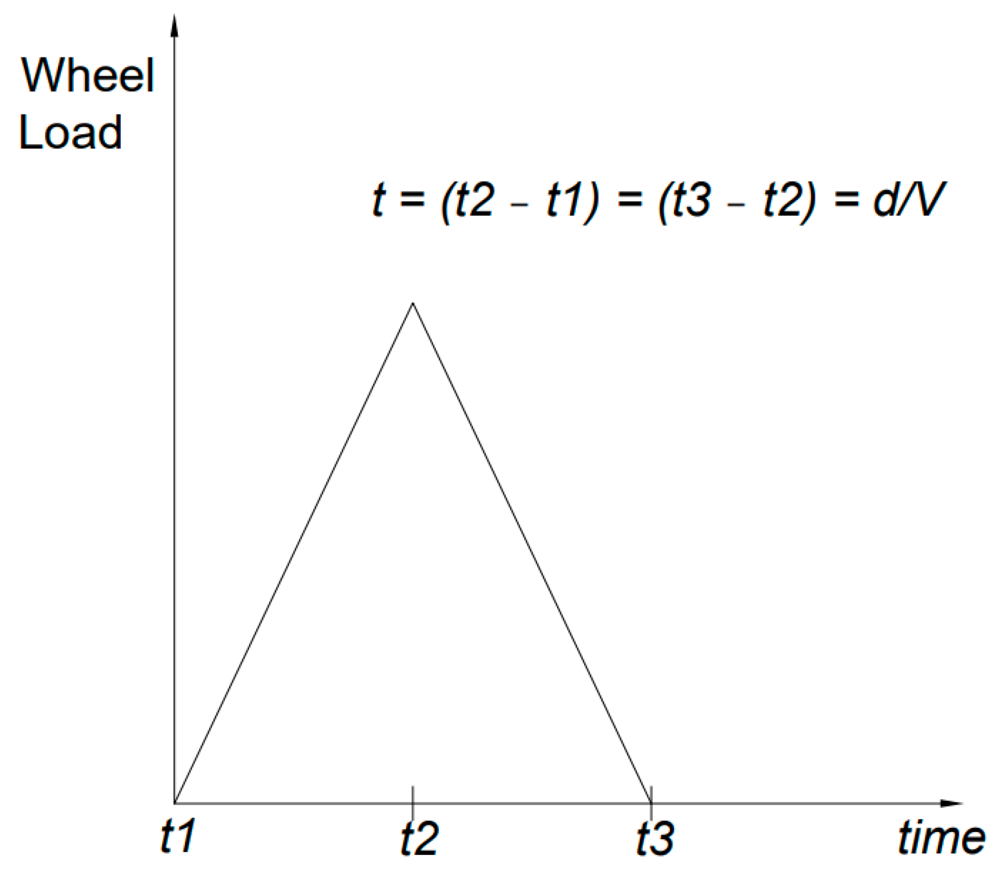
This study uses a series of stepwise activated pulse loads to represent the moving axles of vehicles. Each train’s wheel load is represented as a triangular pulse load (Figure 6). This triangular shape assumes a linear variation of contact force over time at each node, which approximates the rising and falling nature of the dynamic wheel–rail interaction as the wheel approaches, crosses, and moves past a specific point on the bridge. It serves as a simplified yet effective representation of the transient loading behavior caused by moving axles. The triangular profile also helps mitigate numerical instabilities during dynamic simulations, making it suitable for time–history analysis in finite element modeling [34]. The loads were moved forward from the west end of the bridge to the east end of the bridge at a total of 100 discrete steps. The loads were moved by 37.2 cm (14.7 in). The load time (t) is defined by dividing the distance between two consecutive nodes in the FE model of the rail (d) by the desired vehicle traveling speed (V). The integration time was defined in the software using the sub-steps of the load. Figure 6 illustrates the triangular time–history of a moving wheel load, where the load increases from zero to a peak axle loading and then decreases to zero as the wheel crosses a point/node on the bridge.

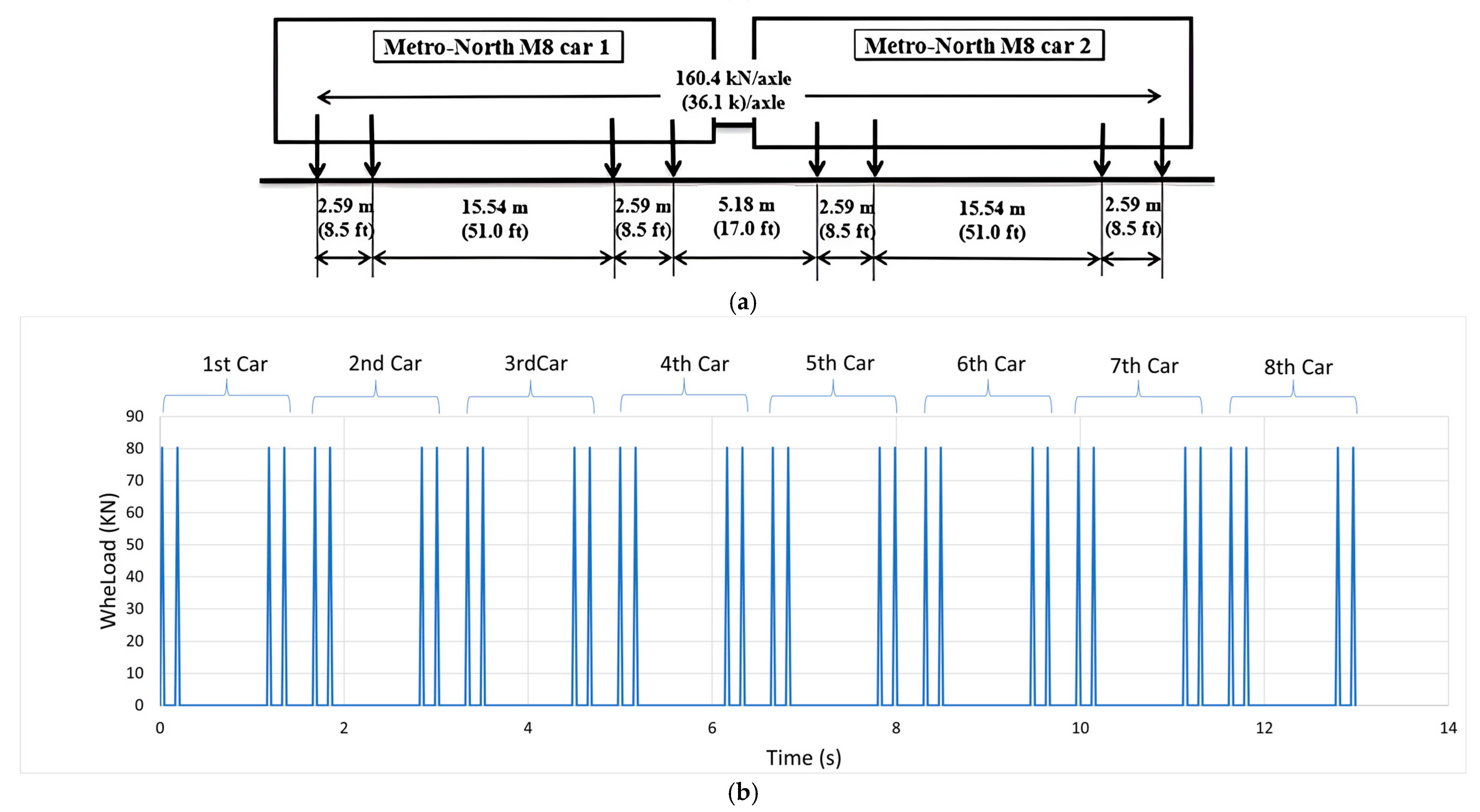
For the preliminary analysis, the Metro-North M8 (MTNR M8) service loading (Figure 7a) is applied in the FE model. Each train’s axle load time was modeled as a triangular load (Figure 7b). The MTNR M8 is an electric multi-axle railroad car built by Kawasaki Rail Car, Inc., for exclusive use on the Metro-North Railroad New Haven Line and the CTrail Shoreline East. The train can reach a maximum speed of 161 km/h (100 mph) and an operational speed of 129 km/h (80 mph). The typical composition is four to five married (double) cars with the same axle load.

3.3. Sensitivity Analysis for Model Updating

Sensitivity analysis is a fundamental step in finite element model updating, enabling the identification of parameters that most significantly influence structural responses such as deflection and natural frequencies. By systematically perturbing uncertain parameters within realistic bounds and observing their effects on key outputs, the analysis prioritizes variables that are both influential and identifiable. This focused approach improves computational efficiency and ensures a well-posed calibration process, particularly important in complex or aging structures where numerous uncertainties exist.

In the case of the Cos Cob Bridge, sensitivity analysis was carried out on a finite element model of span 3, Track 4 to determine which parameters most significantly affected the span’s mid-span deflection and its first few natural frequencies. Based on engineering judgment, structural behavior of truss systems, and insights from prior literature [18,23], the analysis was confined to four critical parameters:

• Young’s Modulus (E) of the steel truss members—initially taken as 2.0 × 10¹¹ Pa for steel but allowed to vary within ±5% (approximately 1.9 × 10¹¹ to 2.1 × 10¹¹ Pa) to account for possible material variability and deterioration effects. This range covers potential reductions in stiffness due to micro-cracking, early steel material variability, or other factors.
• Density (ρ) of the steel—initially 7850 kg/m³, varied between 7000 and 8100 kg/m³. The range was chosen to reflect potential deviations in material density due to construction variations, aging, and corrosion, as well as to ensure an accurate representation of the structure’s mass and inertial properties.
• Cross-Sectional Area of members—a uniform reduction factor was applied to all steel member cross-sectional areas to represent possible section loss (e.g., from corrosion or rivet slip). Based on the visual observation during the site visit and the prior inspection report [35], a maximum cross-sectional area reduction limit of 10% was selected. The reduction factor represents the worst-case cross-sectional deterioration identified and was used as an upper bound for the sensitivity analysis. A negative percentage change indicates a reduction of the nominal cross-sectional area. For example, a −6% change means the member cross-sectional areas are 94% of their original values.
• Support Spring Stiffness (k)—The longitudinal spring at the west-end support simulates translational flexibility, unlike a pinned support that restrains all movement but allows rotation. The stiffness was varied between 50,000 and 250,000 N/mm. The range was determined by comparing vertical displacements from the FEM under two boundary conditions: pinned-roller and fully pinned. The lower bound produced displacement similar to the pinned-roller case, while the upper bound matched the fully pinned condition. This parameter was treated as uncertain and sampled using a log-normal distribution. A similar approach to modeling support flexibility through spring stiffness was adopted by Svendsen et al. [18] in their sensitivity-based bridge model updating.

3.4. Mathematical Formulation

Let θ = [${\theta }_1,{\theta }_1,\dots \dots .{\theta }_n]$ represent the vector of model parameters to be updated (e.g., stiffness, mass, or boundary conditions). The finite element (FE) model predicts system responses ${\mathrm{r}}_{\mathrm{m}\mathrm{o}\mathrm{d}\mathrm{e}\mathrm{l}}\left(\mathsf{\theta }\right)$, and field monitoring provides corresponding measured responses ${\mathrm{r}}_{\mathrm{e}\mathrm{x}\mathrm{p}}.$ The FE model updating task can be performed by minimizing a discrepancy function:

$$\mathsf{\Phi }\left(\mathsf{\theta }\right)=\parallel {\mathrm{r}}_{\mathrm{e}\mathrm{x}\mathrm{p}}-{\mathrm{r}}_{\mathrm{m}\mathrm{o}\mathrm{d}\mathrm{e}\mathrm{l}}\left(\mathsf{\theta }\right)\parallel$$

(1)

where ‖⋅‖ is typically a Euclidean or weighted norm [23,36]. Gradient-based methods approximate the partial derivatives of each model response $r_i$ with respect to each parameter ${\theta }_j,$ entries of the sensitivity matrix S:

$${\mathrm{S}}_{\mathrm{i}\mathrm{j}}={\displaystyle \frac{{\partial \mathrm{r}}_{\mathrm{i}}}{{\partial \mathrm{\theta }}_{\mathrm{j}}}}$$

(2)

These derivatives form the sensitivity matrix, whose structure reveals how variations in parameters influence different outputs. Singular Value Decomposition (SVD) of this matrix can be used to identify rank deficiency or linear dependencies, helping to screen out poorly identifiable parameters [23].

3.5. Iterative Updating Procedure Using Real-Coded Genetic Algorithm (RCGA)

A hybrid approach combining direct sensitivity analysis with a genetic algorithm (GA) was used to update the FE model. Traditional gradient-based algorithms would update the parameter vector ($\mathsf{\theta })$ iteratively; for example, using a steepest-descent type update:

$${\mathsf{\theta }}^{(\mathrm{k}+1)}={\mathsf{\theta }}^{\left(\mathrm{k}\right)}-{\mathsf{\alpha }}^{\left(\mathrm{k}\right)}\left({\mathrm{S}}^{\mathrm{T}}\mathrm{W}\right)\nabla \mathsf{\Phi }\left({\mathsf{\theta }}^{\left(\mathrm{k}\right)}\right)$$

(3)

where α^(k) is a step size, W is a weighting matrix, and ∇Φ is the gradient of the discrepancy function [36]. Alternatively, heuristic approaches (e.g., genetic algorithms) are employed for highly nonlinear parameter spaces [37].

In the RCGA implementation, the optimization began with an initial population of real-valued candidate solutions, each representing a possible set of values for the selected model parameters (e.g., Young’s modulus (E), density (ρ), cross-sectional area (A), and support stiffness (k)). To maintain physical realism while capturing parameter uncertainty, the initial population was generated by random sampling from log-normal distributions centered around nominal values. The log-normal formulation ensured positivity and allowed asymmetric variation, reflecting practical scenarios, such as material degradation or corrosion, that often reduce properties rather than increase them. The evolutionary process proceeded through the following steps:

• Initial Population and Fitness Evaluation: Each candidate’s parameter set was fed into the FE model, and the resulting global responses (vertical peak displacement at different locations) were compared with field measurements. A discrepancy function $\mathsf{\Phi }\left(\mathsf{\theta }\right)$ quantifying the mismatch between model and measured responses was used to evaluate fitness (with lower $\mathsf{\Phi }\left(\mathsf{\theta }\right)$ indicating a better fit).
• Selection of Best Parameters: Using roulette wheel selection, individuals were probabilistically chosen for reproduction based on their fitness. This ensured that better-performing candidates had a higher chance of contributing to the next generation, while maintaining diversity in the gene pool.
• Crossover and Mutation: Selected parent parameter sets underwent crossover (e.g., uniform crossover) to produce offspring (children) by combining genetic material from two parents. Additionally, mutation operations—small random perturbations based on the Gaussian distribution—were applied to explore the parameter space locally and avoid premature convergence.
• Generation of Elite Offspring: The offspring (children) were then combined with the parent population and sorted based on their fitness function to preserve the original population sample size while generating quality offspring. This increases the convergence toward the optimized parameters.

This process was repeated for multiple generations until convergence criteria (ε) were met, either a negligible improvement in fitness between successive generations or the completion of a predefined number of iterations. The resulting optimized parameter set minimizes the discrepancy function $\mathsf{\Phi }\left(\mathsf{\theta }\right)$ and enables the updated FE model to more accurately reproduce the measured global responses.

The GA then evolved the population over successive generations. We used the roulette wheel selection method to probabilistically favor parameter sets with lower discrepancy Φ (better fit) while maintaining diversity in the gene pool. Crossover and mutation operations were applied to create new candidate (children) solutions by combining and randomly altering existing ones. At each generation, the FE model was run for each candidate’s parameter set to compute the fitness (defined inversely by Φ, so lower Φ yields higher fitness). Through this iterative evolutionary process, the GA efficiently explored the parameter space, balancing global search and local refinement. The process was terminated when the improvement between generations became marginal or a preset number of generations was reached. A summary of the key RCGA parameters used in this study is provided in

Table 1. Real-Coded Genetic Algorithm (RCGA) Parameters Used in Sensitivity-Based Model Updating.

Parameter	Value	Justification
Population size	12 sets per iteration	Balances exploration of parameter space and computational cost for FE analysis
Number of Generations	User-defined (until convergence or fitness plateaus)	Allows sufficient refinement of solutions while keeping runtime manageable
Crossover Rate	Arithmetic average (50–50 blend)	Simple, stable method to combine genetic material from two parents
Mutation Rate	5% (per parameter)	Maintains diversity and avoids local optima without disrupting convergence
Initial Distribution	Log-normal distribution	Reflects physical constraints (positivity) and realistic degradation behavior
Selection Method	Roulette Wheel	Ensures probabilistic bias toward better solutions while preserving diversity

. The schematic flowchart of this procedure is provided in Figure 8.

3.6. Convergence and Validation

Model updating concludes when a convergence criterion is met, such as [9,18]:

• Error Tolerance: The norm of the difference between model predictions and experimental results, ‖r_exp − r_model‖, fell below a predefined threshold (indicating an acceptably small discrepancy). In this study, the threshold was set to 1% of the experimental value, which reflects an acceptable level of discrepancy based on typical measurement uncertainty and modeling assumptions used in similar structural calibration studies. This threshold was selected to ensure that the updated finite element model closely replicates the measured structural response without over-fitting.
• Parameter Stability: The changes in parameter values between successive GA generations became very small, suggesting the algorithm had converged on an optimal or near-optimal solution.
• Physical Reasonableness: The optimized parameters remained within realistic engineering limits. In practice, this meant that the GA results were checked to ensure, for example, that the adjusted Young’s modulus was still within a few percent of the expected value for steel, or that the implied section loss or support stiffness was reasonable and could be explained by actual bridge conditions.

Once a converged set of parameters was obtained, the final step was to validate the updated model against independent data or metrics not explicitly used in the calibration. In this study, the validation was performed by comparing the updated model’s predictions to field measurements for different train cases (trains that were not the basis of the optimization) and by checking additional response characteristics like frequencies. Close agreement in these comparisons increases confidence that the model updating improved the model in a general sense rather than over-fitting to a specific scenario.

4. Results

This section presents the vertical displacement results and the natural frequencies of the Cos Cob bridge from FE model analysis using ANSYS and the field testing results obtained using the LDV measurements under the service load of an eight-car MTNR M8 train. The results from these two methodologies have been compared to assess the accuracy of the FE modeling approach.

4.1. Field Testing

The field test data from the LDV (and supplementary accelerometers) were processed to obtain time-domain deflection histories and frequency-domain spectra for span 3 of the Cos Cob Bridge. The Fast Fourier Transform (FFT) was applied to the vibration data to identify the bridge’s natural frequencies from the free vibration response after train passages.

Table 2. Comparison of FEM Model Transient Vertical Peak Deflection and Field Test Results at Different Locations of the Cos Cob Bridge During MTNR M8 Train Passage.

Location	FE Transient Vertical Deflection Results +	Field Test Vertical Displacement Results +	% Difference of FE Results with Respect to the Field Test Results
Vib 1	−3.69 mm	−3.38 mm	9.17%
Vib 2	−3.43 mm	−3.04 mm	12.82%
Vib 3	−2.81 mm	−2.61 mm	7.66%

Note: ⁺ The negative values in columns 2 and 3 represent the vertical downward deflections of the bridge.

compares the peak vertical deflections measured at the mid-span (and other sensor locations) during the train tests with those obtained from the initial FE model simulation under similar loading conditions (same train type and speed). These initial comparisons help establish the baseline accuracy of the FE model prior to calibration.

As shown in Table 2, the initial FE model predicted slightly larger deflections than those observed in the field. The errors ranged from about 7.7% to 12.8%, with the largest discrepancy at the Vib 2 location. These differences, while not enormous, are significant in the context of model validation, and they motivated the subsequent model updating process.

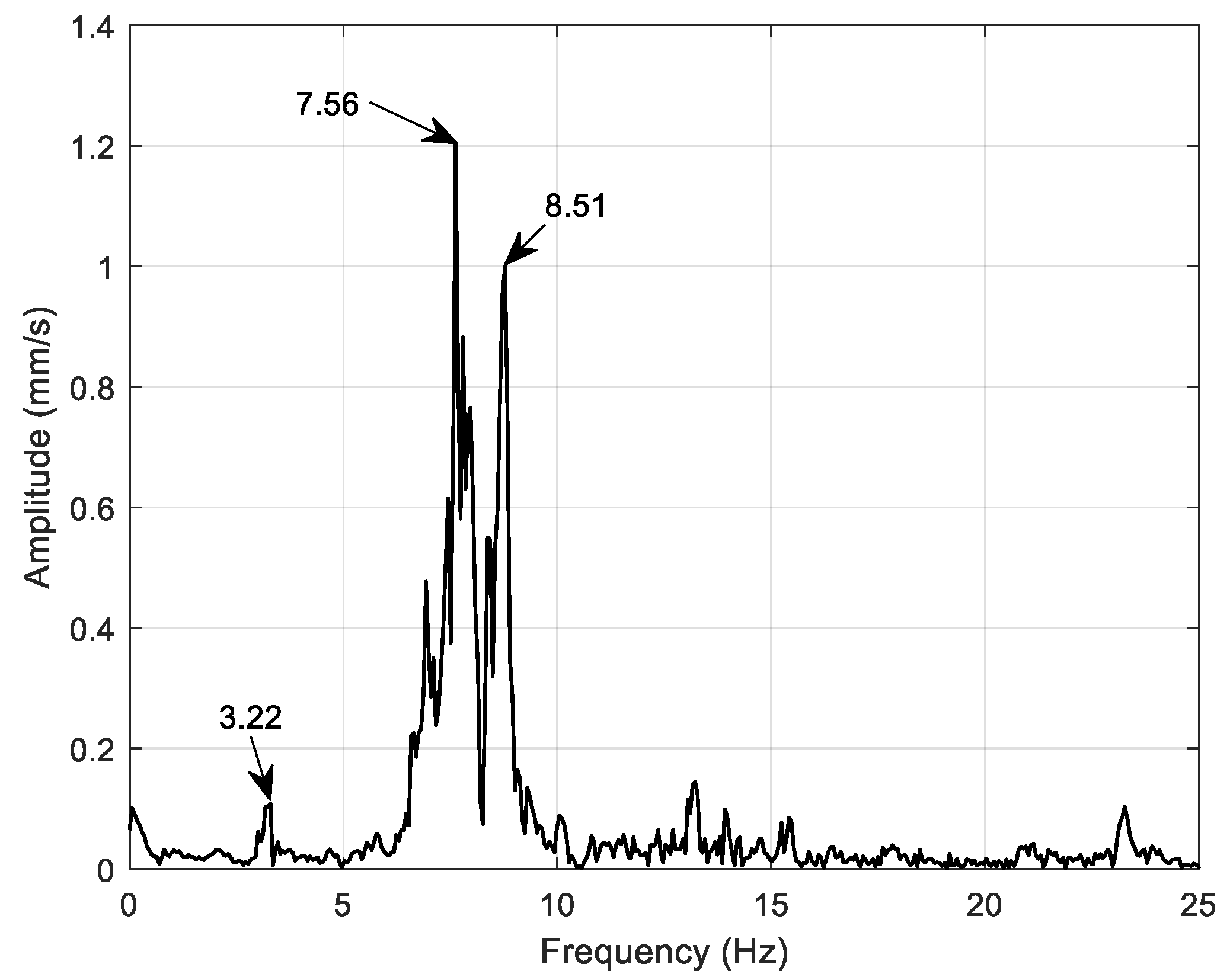
The field vibration data also revealed the bridge’s natural frequencies during free vibration (i.e., after the train had moved off the span).

Table 3. Natural Frequencies of the Cos Cob Bridge During Free Vibration after MTNR M8 Train Passage.

Mode	Natural Frequency (Hz)
	Vib 1	Vib 2	Vib 3
1st Lateral	3.22	3.28	3.31
2nd Lateral	8.51	8.56	8.59
1st Vertical	7.56	7.61	7.65

presents the first three natural frequencies identified from the field measurements (for lateral and vertical modes), after the MTNR M8 train passage. These frequencies were identified using data collected from three different sensor locations: Vib 1, Vib 2, and Vib 3. The frequency values extracted across all sensor locations are very close to each other, indicating that sensor placement had a minimal impact on the results. Figure 9 illustrates the typical frequency spectrum obtained from the LDV data, where peaks corresponding to the bridge’s modal frequencies can be observed.

The initial FE model’s natural frequency predictions were close but not identical to the measured values. For example, the initial model gave a first lateral mode around 3.79 Hz and a first vertical mode around 8.25 Hz, indicating the model was somewhat stiffer than the actual structure (predicting higher frequencies). The second lateral mode from the model was around 8.69 Hz, similarly higher than measured. These discrepancies in both deflection and frequency reinforced the need for model calibration, targeting a reduction of stiffness (or an increase in mass) in the FE model to better match the observed behavior.

4.2. Model Calibration/Updating

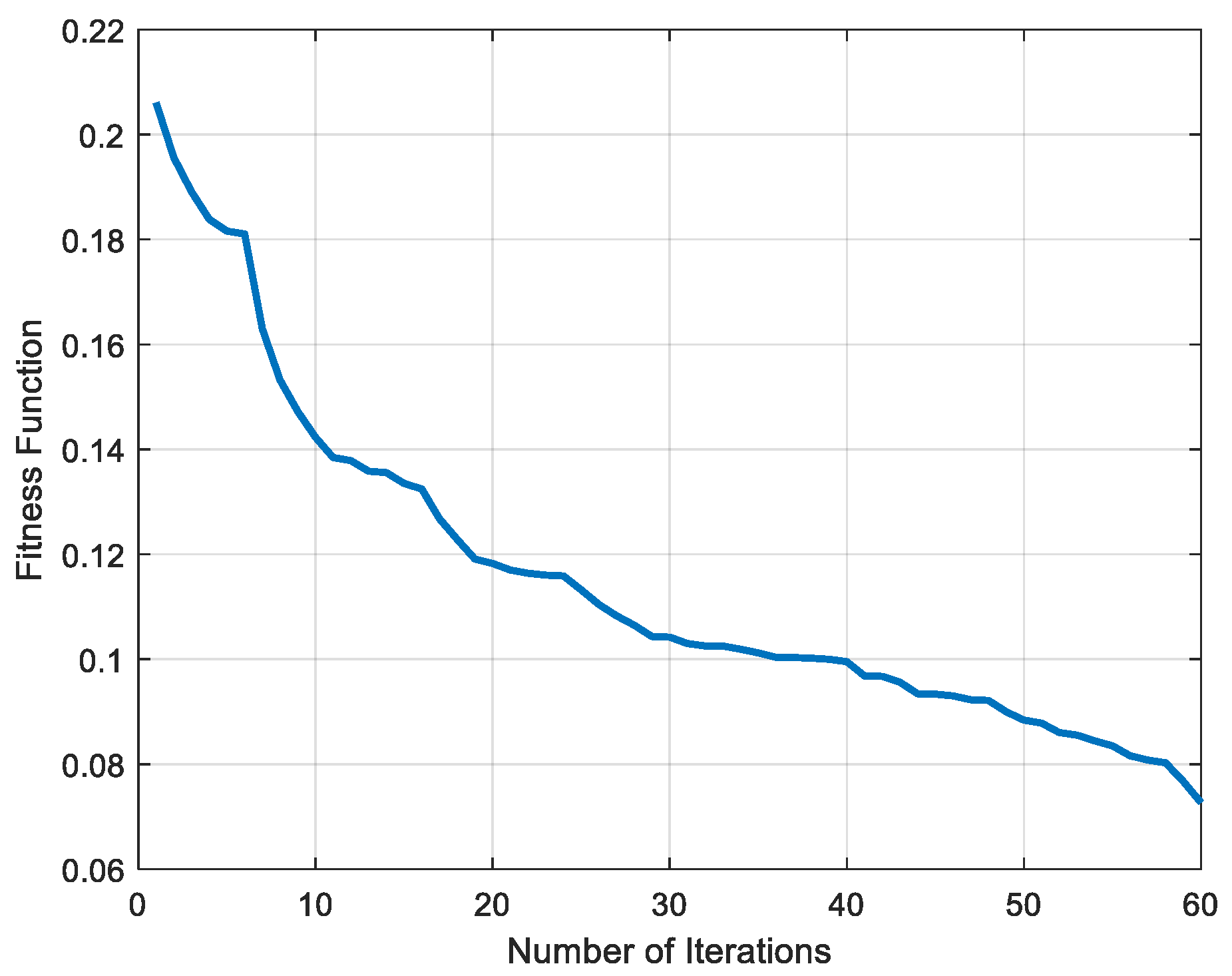
Using the procedure outlined in the Sensitivity Analysis and Model Updating section, a comprehensive sensitivity analysis and optimization were conducted to calibrate the FE model. The analysis confirmed that the parameters identified (steel E, steel density, cross-sectional area reduction, and support spring stiffness) had the most significant impact on the outputs of interest (vertical deflections and frequencies). By integrating an initial broad exploration of the parameter space (via log-normal sampling of the parameters) with the focused optimization of the genetic algorithm, this study efficiently calibrated the model to reflect the real-world behavior of the bridge. The GA’s evolution of the parameter set is illustrated in Figure 10, which plots the fitness function (inversely related to Φ) versus the number of iterations; the curve shows a clear convergence toward an optimal solution. Individual sensitivity curves were not developed in this study, as all parameters were varied simultaneously using a genetic-algorithm-based optimization approach, making it difficult to isolate the effect of a single variable. These curves typically illustrate how a response changes when one parameter varies while others are held constant. Future work may consider one-variable-at-a-time studies to generate such curves and better quantify parameter influence.

Through the sensitivity analysis and GA optimization, the model calibration homed in on a specific set of parameter values that produced the best agreement with the field data. These optimized parameters were as follows:

• Young’s modulus (E): 1.918 × 10¹¹ Pa. This value is about 4% lower than the nominal 2.0 × 10¹¹ Pa for steel, suggesting a slight reduction in effective stiffness of the structure. The reduction plausibly reflects the effects of long-term material degradation, residual stresses, and non-ideal boundary or connection behavior in the century-old Cos Cob Bridge. Factors such as fatigue damage, micro-cracking, and riveted joints may contribute to a slight reduction in the effective stiffness of the structure.
• Density (ρ): 8100 kg/m³. This is higher than the typical steel density of 7850 kg/m³, possibly accounting for additional structural and non-structural mass in the system (for instance, track, fasteners, and other non-structural attachments like electrical components not explicitly modeled). This calibration adjustment effectively lowers the model’s natural frequencies, aligning better with field-measured responses.
• Cross-sectional area change (A%): −6.23%. A small uniform reduction (around 6%) in the cross-sectional areas of members improved the match with observed deflections, consistent with minor section losses from corrosion over time, especially in weather-exposed regions, or an overestimation of section sizes in the original as-built documentation. It may also capture unmodeled eccentricities or fabrication tolerances that reduce effective member stiffness.
• Longitudinal stiffness (k at support): 1.6493 × 10⁵ N/mm. This value represents the optimized stiffness of the west-end support. It indicates that the support is not completely rigid longitudinally; the optimized stiffness suggests a partially flexible support that allows a small amount of movement. This flexibility can occur due to bearing play or deformation of support elements, and adjusting this parameter was important to match the measured deflection and vibration characteristics.

These parameters were obtained through the GA and then input into the ANSYS FE model for verification. With the updated parameters, the FE model was re-run to predict the bridge’s response under the same loading scenarios as the field tests.

4.3. Updated FE Model

Following the sensitivity analysis and GA optimization, the FE model of the Cos Cob Bridge was updated with the optimized parameter values listed above. The final step was to compare the updated model’s responses against the field measurements (and against the initial model results) to quantify the improvements achieved through calibration.

The primary focus was on the vertical deflection responses at the three instrumented locations (Vib 1, Vib 2, Vib 3) under the crossing of a Metro-North M8 train, as this scenario was used to drive the optimization.

Table 4. Comparison of Peak Vertical Deflection Results of the Cos Cob Bridge with Field Test, Initial FE Model, and Optimized FE Model under Different Train Loadings.

Train Type	Location	Field Test Max Deflection (mm) +	Initial FE Max. Deflection (mm) +*	Updated FE Max Deflection (mm) +*
Metro North M8	Vib 1	−3.38	−3.69 (9.17%)	−3.24 (4.14%)
	Vib 2	−3.04	−3.43 (12.82%)	−3.13 (2.96%)
	Vib 3	−2.61	−2.81 (7.66%)	−2.58 (1.14%)
AMTRAK Acela	Vib 2	−4.581	−6.131 (33.835%)	−5.191 (13.315%)
AMTRK Regional	Vib 2	−4.413	−5.889 (33.446%)	−4.841(9.698%)

Note: ⁺ The negative values in columns 3, 4, and 5 represent the vertical downward deflection of the bridge. * The percentage shown in columns 4 and 5 represents the percentage difference of the peak deflections from the FE model predictions (initial and updated) with respect to the field test maximum deflection values.

presents the peak vertical deflections at those locations from the field test, the initial FE model, and the updated FE model for the M8 train case. Figure 11 provides the full time–history curves of vertical deflection at Vib 1, Vib 2, and Vib 3 from both the field test and the updated FE model (showing a close overlap).

As seen in Table 4, the updated FE model’s deflection predictions show a marked improvement over the initial model at different locations at different speeds of trains. For the M8 train, the initial model over-predicted the deflection at Vib 2 by about 12.8%, whereas the updated model’s prediction is within 3% of the measured value. Similar improvements were observed at Vib 1 and Vib 3: the initial errors of 9.2% and 7.7% were reduced to about 4.1% and 1.1%, respectively. The direction of correction is consistent—the initial model was generally too stiff (producing smaller deflections than measured), and the calibration reduced the stiffness such that deflections increased and matched the field values more closely. Figure 11a–c illustrate these comparisons graphically for the M8 train case at three different locations, with the updated model’s deflection curves nearly overlapping the field curves.

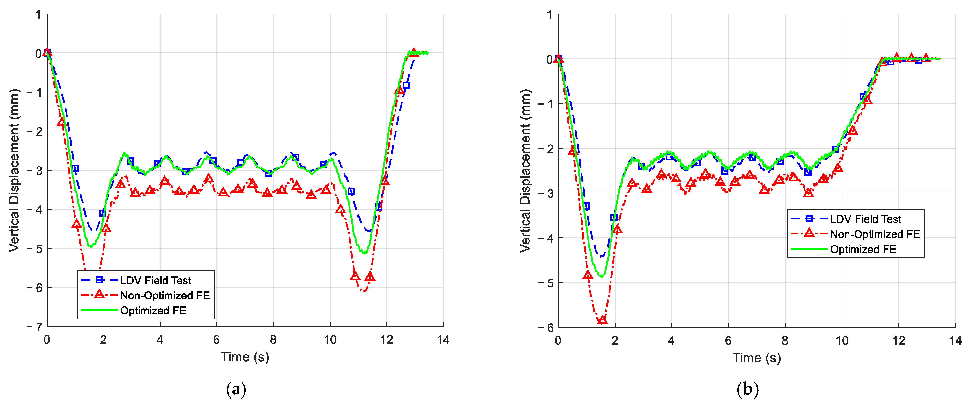
After confirming the updated model’s accuracy for the M8 loading (which was used for calibration), the model was further validated using the two Amtrak train cases (Amtrak Regional and Acela Express) that were also recorded during field testing. These cases serve as independent checks because they involve different total loads, axle spacing, and speeds. The updated model was subjected to the Amtrak Regional and Acela load cases (using the same calibrated parameters, with the only difference being the loading inputs). Figure 12a,b show the axle load configurations for the Amtrak Regional and Acela trains that were used in the analysis. The results, included in Table 4 for Vib 2, show that the updated model also performed well for these scenarios. For the Amtrak Acela (a high-speed trainset with a different axle configuration), the initial model’s peak deflection error at mid-span was quite large (~33.8%), whereas the updated model cut that error to about 13.3%. For the Amtrak Regional locomotive, the error dropped from ~33.4% to ~9.7% after calibration. The larger initial errors for the Amtrak trains suggest that the initial model’s assumptions (especially regarding dynamic amplification or support stiffness) might not have been adequate for heavier or faster trains, but the updated model, calibrated primarily on the M8 data, generalized well to these cases. Figure 13a,b compare the updated FE model and field deflection time histories at Vib 2 for those trains. The updated model captures the peak deflections and overall response shape reasonably for both train loading cases.

In addition to deflections, the first few natural frequencies of the updated FE model were computed and compared to the field-identified values (from Table 3).

Table 5. Comparison Table of Natural Frequencies of the Cos Cob Bridge.

Mode	Natural Frequency (Hz)
	Field Test	Initial FE Result	% Difference *	Optimized FE Result	% Difference *
1st Lateral	3.22	3.79	17.70	3.31	2.795
2nd Lateral	8.51	8.69	2.12	8.43	−0.940
1st Vertical	7.56	8.25	9.13	7.78	2.910

Note: * Column 4 and 6 display the % difference values of the initial and optimized FE results with respect to those from the field tests, respectively. The negative (minus) sign in front of a % value indicates that the FE result is less than that from the field test.

summarizes the comparison of the three primary modal frequencies before and after model updating. The initial FE model frequencies are included along with the percentage errors relative to the field values, and the same is performed for the updated model frequencies. The updated model frequencies show much smaller errors, indicating that the model’s dynamic characteristics have been successfully tuned.

The improvement in frequency prediction can be attributed to the adjustments in E (reducing stiffness) and ρ (increasing mass) in the calibration process. The slightly increased density used in the model is justified by the cumulative mass of structural and non-structural components not explicitly captured in the model. These include fasteners, rivets, gusset plates, instrumentation cables, and additional steel components likely added during the rehabilitation process over the years. The close agreement across both lateral and vertical modes suggests that the calibration did not over-fit to just one mode but rather achieved a balanced adjustment that benefits the overall dynamic behavior.

The results of this study confirm the effectiveness of the proposed updating method. Unlike the digital twin approaches by Lai et al. [17], which use continuous SHM data for Bayesian forecasting, and Nhamage et al. [13], which combine BIM and real-time fatigue simulation, this study achieves similar accuracy through a simpler, data-sparse approach. While those methods offer predictive capabilities and detailed visualization, our results show that reliable model calibration is still possible without continuous monitoring, making it well-suited for aging bridges with limited instrumentation.

Overall, the updated FE model of the Cos Cob Bridge shows significantly better agreement with real behavior, both in static/dynamic deflections under trains and in free vibration characteristics, compared to the initial model. These improvements validate the effectiveness of the sensitivity-driven, GA-based updating framework in aligning simulated and observed bridge responses. The calibrated model can now be used with more confidence for further analysis, such as fatigue life estimation, load rating under various train loadings, or studying the effects of hypothetical strengthening or deterioration scenarios.

5. Conclusions

The finite element model of the railroad bridge structure selected was successfully calibrated against field test results through a sensitivity analysis and genetic-algorithm-based updating procedure, yielding substantial improvements in predictive accuracy. Quantitatively, the updated model reduced peak deflection prediction errors from initial discrepancies of 7–34% down to within 1–14% across instrumented locations for different train loadings. Similarly, errors in natural frequency predictions by the updated FE model decreased from approximately 10–18% in the baseline model to under 3% after updating. These gains were achieved by refining key parameters: the effective Young’s modulus was reduced by approximately 4%, reflecting minor stiffness degradation; the modeled density was adjusted upward by about 3%, capturing unmodeled mass contributions; and the longitudinal support stiffness increased nearly twofold, reflecting actual restraint behavior observed in the field. Together, these calibrated parameters enabled the model to closely match measured deflection time histories and dynamic characteristics under multiple train load cases, validating its robustness and transferability.

The updated model now serves as a reliable tool for structural response prediction, load rating estimation, and fatigue life assessment, supporting informed maintenance decisions. Although this study focused on a specific steel truss railroad bridge, the overall methodology, combining field measurements, sensitivity analysis, and model updating, is broadly applicable to other aging structures. Since the approach relies on commonly available structural data and does not require permanent monitoring systems, it can be adapted to various bridge types or infrastructure systems where detailed modeling and data-driven calibration are needed. Its computational efficiency and reliance on limited but high-quality data make it suitable for application in scenarios where permanent monitoring systems are not feasible.

However, it must be pointed out that the numerical model was developed primarily to capture the global dynamic response of the bridge superstructure; therefore, details about track-related components, such as rail cross-section geometry, fastening system behavior, and longitudinal track resistance, were not explicitly included. These elements can influence the overall system stiffness and dynamic behavior [38] but were excluded due to limited field data and to maintain focus on primary structural parameters. Additionally, due to equipment constraints, only a single LDV was used and repositioned across three locations, which limits the spatial resolution of measured responses and may not fully capture complex modal behaviors. Therefore, the methodology can be further improved in the future by employing multi-point LDV systems and refined modeling of track, rail–track structure, and connection-related parameters mentioned above.

Furthermore, developing localized FE sub-models near critical connections or gusset plates could enhance the detection of fatigue-prone or damage-sensitive areas. Long-term monitoring and fatigue analysis using cumulative loading histories could also provide more comprehensive service life predictions. These additions would enhance model fidelity while maintaining practical applicability for infrastructure resilience planning.