A Finite Element Formulation for True Coupled Modal Analysis and Nonlinear Seismic Modeling of Dam–Reservoir–Foundation Systems: Application to an Arch Dam and Validation

Abstract

This paper presents a formulation for the dynamic analysis of dam–reservoir–foundation systems, employing a coupled finite element model that integrates displacements and reservoir pressures. An innovative coupled approach, without separating the solid and fluid equations, is proposed to directly solve the single non-symmetrical governing equation for the whole system with non-proportional damping. For the modal analysis, a state–space method is adopted to solve the coupled eigenproblem, and complex eigenvalues and eigenvectors are computed, corresponding to non-stationary vibration modes. For the seismic analysis, a time-stepping method is applied to the coupled dynamic equation, and the stress–transfer method is introduced to simulate the nonlinear behavior, innovatively combining a constitutive joint model and a concrete damage model with softening and two independent scalar damage variables (tension and compression). This formulation is implemented in the computer program DamDySSA5.0, developed by the authors. To validate the formulation, this paper provides the experimental and numerical results in the case of the Cahora Bassa dam, instrumented in 2010 with a continuous vibration monitoring system designed by the authors. The good comparison achieved between the monitoring data and the dam–reservoir–foundation model shows that the formulation is suitable for simulating the modal response (natural frequencies and mode shapes) for different reservoir water levels and the seismic response under low-intensity earthquakes, using accelerograms measured at the dam base as input. Additionally, the dam’s nonlinear seismic response is simulated under an artificial accelerogram of increasing intensity, showing the structural effects due to vertical joint movements (release of arch tensions near the crest) and the concrete damage evolution.

1. Introduction

The numerical modeling of the dynamic behavior of concrete dams remains one of the most challenging and important topics in dam engineering [1,2], which requires the development of sophisticated and robust finite element models for simulating the dam–reservoir–foundation system, considering the main dynamic interaction effects [3,4,5,6,7,8,9,10,11] (including damping phenomena). These models can be calibrated through comparison with the experimental modal response of the dam [12,13,14,15,16,17], obtained from vibrations measured under ambient/operational excitation, and with the structural response recorded during seismic events [16,17,18,19,20,21,22]. Once properly validated, the models can be used to support structural health monitoring over time [23] and to simulate dam response under earthquakes of different intensities. For predicting the response under strong earthquakes, these models should be further developed to account for nonlinear structural behavior [24,25,26,27,28,29], using appropriate constitutive models to simulate the structural effects due to joint movements [24,26,30,31,32,33] and the behavior of concrete, up to failure, under both tension and compression [34,35,36,37,38]. The nonlinear models can then be applied in seismic design and safety assessment studies.

A key issue in the development of finite element models for dynamic analysis of dam–reservoir–foundation systems is the simulation of the reservoir and the dam–reservoir dynamic interaction. Extensive research has been conducted on this topic, leading to the development of two main well-established approaches. The classic added water mass models, generally adopted due to their simplicity and efficiency, simulate the reservoir based on the solution proposed by Westergaard [39], and later improved by Kuo [40], by calculating water masses equivalent to the hydrodynamic pressures on the upstream dam face. However, this type of model involves certain simplifying assumptions (e.g., rigid dams with vertical upstream faces) that can affect the results in both modal analysis and seismic response simulations [5,17,27,41,42,43,44]. In the case of arch dams, the added water mass effect is overestimated by models based on Westergaard’s solution, making it necessary to apply added mass reduction factors of about 50 to 70% [1,2]. A more advanced modeling approach is the one based on the coupled formulation, proposed by Zienkiewicz [45]. Coupled models use displacement finite elements for the dam–foundation domain and pressure (or velocity potential) fluid finite elements for simulating the reservoir, enabling the consideration of dam motion–water pressure coupling, the surface wave effects, and the pressure wave propagation with radiation damping at the far-end [8,42,46,47]. Although coupled models are more complex and computationally demanding, as they require the reservoir to be discretized, they allow better predictions of the experimental modal parameters of arch dams simply by adjusting the elasticity modulus of the concrete and the pressure wave propagation velocity in the reservoir [16,29]. Also, the use of a discretized reservoir with fluid elements, considering water compressibility, is recommended in most cases, avoiding the overestimation of the dam response [27].

In this work, a coupled model is adopted for modeling the reservoir and the dam–reservoir interaction. However, coupled formulations originate non-symmetrical problems due to the solid–fluid coupling term that establishes the relation between the solid and fluid equations [45,48]. For this reason, specific methods are required for calculating the dynamic response of dam–reservoir–foundation systems based on coupled models. The traditional approach involves separating the solid and fluid equations and subsequently symmetrizing the dynamic coupled problem, using the simplified hypothesis of Rayleigh damping proportional to mass and stiffness. This is performed for both the modal analysis [46,49,50,51,52,53] and for the time domain dynamic response calculation [48,54]. For example, traditional modal analysis methods involve the separate calculation of dam–foundation modes and reservoir modes. Also, damping is usually neglected, which produces real eigenvalues and eigenvectors, resulting in undamped stationary modes. Therefore, the main goal of this paper is to present an alternative, innovative approach to solve the dynamic coupled problem for dam–reservoir–foundation systems, as well as calculation methods with several novel aspects, for modal analysis and nonlinear seismic analysis.

Specifically, a true coupled approach, without separating the solid and fluid equations, is proposed to directly solve the non-symmetrical finite element coupled equation for the global dam–reservoir–foundation system. This approach makes it possible to compute the dynamic response with generalized damping, i.e., considering non-proportional damping in the dam–foundation domain and radiation damping in the reservoir. The possibility of assuming damping in the dam body that is not proportional to its stiffness enables the incorporation of sets of elements with different material properties in the model, which is an important advantage for predicting the dynamic behavior of dams that have deteriorated zones (usually associated with lower stiffness and higher damping).

In addition, a complete finite element formulation based on the true coupled approach is developed for modal analysis and for seismic response simulation. For the modal analysis, the state–space method is pioneeringly adopted to solve the coupled eigenproblem of the dam–reservoir–foundation system with damping: complex eigenvalues and eigenvectors are computed, which correspond, physically, to damped vibration modes with non-stationary nodes [55] (this type of vibration mode has been identified from vibrations measured on large concrete dams [10,16,56]). For the seismic response analysis, a Newmark-based time-stepping method is applied to the coupled dynamic equation for the system, in order to calculate the structural response in displacements and the hydrodynamic pressures in the reservoir. A stress–transfer iterative method, innovatively divided into two subroutines, is incorporated into the time-stepping algorithm to simulate nonlinear structural behavior, combining a constitutive joint model and a concrete damage model with softening and two independent damage variables (one for tension and the other for compression). A key motivating factor for developing this formulation was its computational implementation in the computer program developed by the authors, DamDySSA, ensuring total knowledge and control over all parameters and details involved, while also facilitating the customization of post-processing tools for the 3D visualization of results [29].

This paper also contributes by providing both experimental and numerical results for a real large arch dam. The goal is to validate the implemented coupled model and demonstrate the suitability of the developed formulation for simulating the modal response and the seismic behavior of dam–reservoir–foundation systems. The case study is the Cahora Bassa dam, instrumented in 2010 with a continuous vibration monitoring system (designed by the authors). First, a calibrated 3D model for the dam–reservoir–foundation system is used to reproduce the evolution of the natural frequencies and the corresponding mode shapes for different reservoir water levels. The results are validated against the experimental modal parameters obtained from vibrations measured continuously on the dam between 2010 and 2023, for three vibration modes. This model is then used in a linear seismic analysis to simulate the accelerations measured at the crest during a real, low-intensity earthquake. A good prediction is achieved by using the accelerograms measured at the dam base as input and assuming a reasonable damping ratio for the first natural frequency in the model. Finally, the model is further developed by incorporating the vertical contraction joints in the dam body and a constitutive damage model for the concrete in order to carry out nonlinear seismic analyses. The dam’s response is simulated under an artificial seismic action of increasing intensity to assess the effects of the vertical joint movements in the structural response and to control the progression of tensile/compressive damage.

This paper is organized as follows. Section 2 presents the coupled model adopted for simulating the dam–reservoir interaction, including the main governing equations and the resulting finite element formulation. Section 3 focuses on the proposed coupled approach for the dynamic analysis of dam–reservoir–foundation systems. It describes in detail the state–space method for modal analysis and the time-stepping methods for linear and nonlinear seismic analysis. Section 4 sets out the validation of the proposed formulation, providing experimental and numerical results of applications conducted in the case study of the 170 m high Cahora Bassa arch dam. Section 5 provides a discussion on the proposed formulation and the presented results. This paper ends with concluding remarks in Section 6.

2. Coupled Model: Dam–Reservoir Interaction

2.1. Governing Equations

A coupled model formulation is used to simulate the dynamic behavior of the dam–reservoir–foundation system [48,54], considering the fluid–structure interaction (Figure 1). The governing differential equations for the solid domain ${\Omega }_s$ (dam–foundation) and for the fluid domain ${\Omega }_w$ (reservoir) are

$${\underset{¯}{\mathit{L}}}^{\mathrm{T}}\left(\underset{¯}{D}\underset{¯}{\mathit{L}}\underset{˜}{u} \right)+\underset{˜}{f}=\underset{˜}{0},\hspace{1em}\forall \hspace{0.33em}{P}_s\in {\Omega }_s,\hspace{0.33em}\hspace{0.33em}\forall \hspace{0.33em}t$$

(1)

$${\nabla }^{2}p-{\displaystyle \frac{\ddot{p}}{c_w^2}}=0,\hspace{1em}\forall \hspace{0.33em}{P}_w\in {\Omega }_w,\hspace{0.33em}\hspace{0.33em}\forall \hspace{0.33em}t$$

(2)

and the boundary conditions prescribed at the main interfaces of the system are

$$\left\{\begin{array}{l}\underset{˜}{u}=\underset{˜}{0}\hspace{1em}\hspace{1em}\hspace{1em}\hspace{0.33em},\hspace{0.33em}{\Gamma }_f\\ \underset{˜}{\mathbf{t}}={\underset{˜}{n}}_{{\Gamma }_{\mathbf{t}}}^{\mathrm{T}}{\gamma }_w{h}_w\hspace{0.33em} \hspace{0.33em},\hspace{0.33em}{\Gamma }_1\end{array}\right.\hspace{1em}\hspace{0.33em}\hspace{1em}\left\{\begin{array}{c}{\displaystyle \frac{\partial p}{\partial {\underset{˜}{n}}_{{\Gamma }_1}}}=-{\rho }_w{\underset{˜}{n}}_{{\Gamma }_1}^{\mathrm{T}}\ddot{\underset{˜}{u}}\hspace{1em}, {\Gamma }_1\\ {\displaystyle \frac{\partial p}{\partial {\underset{˜}{n}}_{{\Gamma }_2}}}={\underset{˜}{n}}_{{\Gamma }_2}^{\mathrm{T}} \ddot{\underset{˜}{u}}=0\hspace{1em}\hspace{0.33em}, {\Gamma }_2\end{array}\right.\hspace{1em}\hspace{0.33em}\hspace{1em}\left\{\begin{array}{l}p=0\hspace{1em}\hspace{1em}\hspace{1em}\hspace{1em}\hspace{0.33em}, {\Gamma }_3\hfill \\ {\displaystyle \frac{\partial p}{\partial {\underset{˜}{n}}_{{\Gamma }_4}}}=-{\displaystyle \frac{1}{c_w}}\dot{p}\hspace{1em}, {\Gamma }_4\hfill \end{array}\right.$$

(3)

The unknowns of this coupled problem are the displacement vector $\underset{˜}{u}=\underset{˜}{u}(x_1,x_2,x_3,t)$ for points $P_s(x_1,x_2,x_3)$ belonging to the solid domain, and the hydrodynamic pressure value, $p=p(x_1,x_2,x_3,t)$, for each point $P_w(x_1,x_2,x_3)$ within the fluid domain. To simplify the presented notation, the spatial and time indices are omitted unless necessary.

Equation (1), or Navier’s equilibrium equation, is used to define the relationship between displacements and forces in the solid domain. In this equation, $\underset{¯}{\mathit{L}}$ is a matrix differential operation that gives the relation between the strains and the three displacement components. The elasticity matrix $\underset{¯}{D}$ is used to correlate the stresses and strains, assuming the isotropic materials hypothesis, and it is written in terms of the material bulk and shear moduli $K=E/3\left(1-2v\right)$ and $G=E/2\left(1+v\right)$, where E is the elasticity modulus and v is Poisson’s ratio. The vector of body forces, $\underset{˜}{f}=\underset{˜}{f}(x_1,x_2,x_3,t)$, includes gravity, inertia, and damping forces. For the dynamic analysis under seismic loading, the body forces become $\underset{˜}{f}={\rho }_s\underset{˜}{g}-{\rho }_s(\underset{˜}{\ddot{u}}+{\underset{˜}{a}}_S)-c_s\underset{˜}{\dot{u}}$, where $\underset{˜}{\dot{u}}$ and $\underset{˜}{\ddot{u}}$ are the velocity and acceleration vectors, ${\rho }_s$ represents the mass density of the solid (dam–foundation) materials, $\underset{˜}{g}$ is the gravity acceleration vector, $c_s$ indicates the specific material damping, and, lastly, ${\underset{˜}{a}}_S={\underset{˜}{a}}_S(x_1,x_2,x_3,t)$ represents the seismic accelerations.

The pressure wave governing Equation (2) is established for the fluid domain assuming the hypothesis of inviscid and compressible fluid [48], where $c_w=\sqrt{K_w/{\rho }_w}$ is the speed of the pressure waves’ propagation in the reservoir, which is related to the water bulk modulus, K_w, and density, ρ_w. For dam reservoirs, appropriate values for the speed of sound in water may vary between 1400 m/s and 1600 m/s, depending on the average water temperature [16].

Regarding the boundary conditions in the dam–foundation domain, a displacement boundary condition is defined by prescribing null displacements for the points at the base of the foundation block ${\Gamma }_f$, while a stress boundary condition is considered by applying forces (or tensions) at the upstream face of the dam ${\Gamma }_1$ to simulate the hydrostatic water pressures. The boundary conditions adopted to simulate the reservoir dynamic behavior and the fluid–structure interaction are the same as in the work by Zienkiewicz et al. [48]. To model the solid–fluid motion coupling, the dam–reservoir interaction is considered by relating pressure gradients and structural accelerations at the dam–water interface ${\Gamma }_1$, while at the reservoir bottom ${\Gamma }_2$, it is assumed that only horizontal motion exists. To account for the effect of the reservoir domain “termination” in the model, a radiation boundary is introduced at the far end boundary of the reservoir ${\Gamma }_4$, assuming only outgoing pressure waves. Finally, a null pressure condition is prescribed at the free surface of the reservoir ${\Gamma }_3$. The normal vector to each interface ${\Gamma }_i$ is given by ${\underset{˜}{n}}_{{\Gamma }_i}$.

2.2. Finite Element Formulation

The coupled problem is discretized using displacement-based finite elements for the dam and foundation, with three displacement degrees of freedom per node, and pressure-based fluid finite elements for the reservoir. Based on the Finite Element Method (FEM) [48], the numerical solutions of the coupled problem (displacements and pressures) are computed for all points of the discretized system in the standard manner: the displacements vector on each point in the solid domain is approximated as $\underset{˜}{u}={\underset{\_}{\mathrm{N}}}_u{\underset{˜}{u}}^{\mathrm{e}}$, and similarly, the pressure value on each point in the reservoir is obtained as $p={\underset{\_}{\mathrm{N}}}_p{\underset{˜}{p}}^{\mathrm{e}}$, where ${\underset{˜}{u}}^{\mathrm{e}}$ and ${\underset{˜}{p}}^{\mathrm{e}}$ are nodal parameters, while ${\underset{\_}{\mathrm{N}}}_u$ and ${\underset{\_}{\mathrm{N}}}_p$ are the matrices containing the values of the interpolation functions. Following the FEM procedure [48], these approximations are introduced in the weak form in the governing Equations (1) and (2), considering the boundary conditions in (3). This makes it possible to obtain the global matrices and force vectors in the dam–foundation and reservoir domains, and therefore, to write the discrete solid and fluid dynamic equations describing the structural motion and the reservoir pressures

$$\underset{¯}{\mathrm{m}}\underset{˜}{\overset{¨}{\mathrm{u}}}+\underset{¯}{\mathrm{c}}\underset{˜}{\overset{\dot{}}{\mathrm{u}}}+\underset{¯}{\mathrm{k}}\underset{˜}{\mathrm{u}}={\underset{˜}{F}}_s+\underset{¯}{\mathrm{Q}}\underset{˜}{\mathrm{p}}$$

(4)

$$\underset{¯}{\mathrm{S}}\underset{˜}{\overset{¨}{\mathrm{p}}}+\underset{¯}{\mathrm{R}}\underset{˜}{\overset{\dot{}}{\mathrm{p}}}+\underset{¯}{\mathrm{H}}\underset{˜}{\mathrm{p}}={\underset{˜}{F}}_w-{\rho }_w{\underset{¯}{\mathrm{Q}}}^{\mathrm{T}} \underset{˜}{\overset{¨}{\mathrm{u}}}$$

(5)

which can be presented in the coupled matrix form as

$$\left[\begin{array}{cc}\underset{¯}{\mathrm{m}}& \underset{¯}{0}\\ {\rho }_w{\underset{¯}{\mathrm{Q}}}^{\mathrm{T}}& \underset{¯}{\mathrm{S}}\end{array}\right]\left[\begin{array}{c}\underset{˜}{\overset{¨}{\mathrm{u}}}\\ \underset{˜}{\overset{¨}{\mathrm{p}}}\end{array}\right]+\left[\begin{array}{cc}\underset{¯}{\mathrm{c}}& \underset{¯}{0}\\ \underset{¯}{0}& \underset{¯}{\mathrm{R}}\end{array}\right]\left[\begin{array}{c}\underset{˜}{\overset{\dot{}}{\mathrm{u}}}\\ \underset{˜}{\overset{\dot{}}{\mathrm{p}}}\end{array}\right]+\left[\begin{array}{cc}\underset{¯}{\mathrm{k}}& -\underset{¯}{\mathrm{Q}}\\ \underset{¯}{0}& \underset{¯}{\mathrm{H}}\end{array}\right]\left[\begin{array}{c}\underset{˜}{\mathrm{u}}\\ \underset{˜}{\mathrm{p}}\end{array}\right]=\left[\begin{array}{c}{\underset{˜}{F}}_s\\ {\underset{˜}{F}}_w\end{array}\right]$$

(6)

The main variables are the displacements vector for the dam–foundation nodes, $\underset{˜}{\mathrm{u}}=\underset{˜}{\mathrm{u}}(t)$(n_s × 1), and the hydrodynamic pressures vector for the reservoir nodes, $\mathrm{p}=\mathrm{p}(t)$ (n_w × 1); the number of degrees of freedom of the global discretized system, n, is equal to the sum of the displacement (n_s) and pressure (n_p) degrees of freedom, n = n_s + n_w. The mass, damping, and stiffness matrices are $\underset{\_}{\mathrm{m}}$, $\underset{\_}{\mathrm{c}}$, and $\underset{\_}{\mathrm{K}}$ (n_s × n_s) for the solid domain, and $\underset{\_}{\mathrm{S}}$, $\underset{\_}{\mathrm{R}}$, and $\underset{\_}{\mathrm{H}}$ (n_w × n_w) for the reservoir domain, while $\underset{¯}{\mathrm{Q}}$ (n_w × n_s) is the coupling matrix that accounts for the water pressure–structure motion coupling. The nodal force vectors in the solid and fluid are, respectively, ${\underset{˜}{F}}_s={\underset{˜}{F}}_s(t)$ (n_s × 1) and ${\underset{˜}{F}}_w={\underset{˜}{F}}_w(t)$ (n_w × 1). The forces applied to the dam may include the dam’s self-weight, the hydrostatic pressure on the upstream face, and the dynamic loads. In the case of dynamic analysis under seismic loading, and omitting other excitation sources, the solid and fluid forces become ${\underset{˜}{F}}_s=-\underset{¯}{\mathrm{m}}\underset{¯}{s}{\underset{˜}{a}}_S$ and ${\underset{˜}{F}}_w=-{\rho }_w{\underset{¯}{\mathrm{Q}}}^{\mathrm{T}}\underset{¯}{s}{\underset{˜}{a}}_S$, where ${\underset{˜}{a}}_S={\underset{˜}{a}}_S(t)$ (3 × 1) is the seismic input, which includes three acceleration time histories in the upstream–downstream, cross-valley, and vertical directions, and $\underset{\_}{s}$ (n_s × 3) is a matrix that distributes the seismic accelerations through all the degrees of freedom.

3. Proposed Coupled Finite Element Formulation

3.1. Coupled Approach with Generalized Damping

In this paper, an innovative true coupled approach is proposed for directly solving the non-symmetrical dynamic equation in a discrete dam–reservoir–foundation system (6), without separating the solid and fluid equations. Based on this approach, a new variable $\underset{˜}{\mathrm{q}}$, which includes the displacement and pressure variables, is defined as the global unknown of the coupled problem

$$\underset{˜}{\mathrm{q}}=\left[\begin{array}{c}\underset{˜}{\mathrm{u}}\\ \underset{˜}{\mathrm{p}}\end{array}\right]$$

(7)

Therefore, the discrete dynamic equation for the dam–reservoir–foundation system is defined as

$$\underset{\_}{\mathrm{M}}\hspace{0.33em}\underset{˜}{\overset{¨}{\mathrm{q}}}+\underset{\_}{\mathrm{C}}\hspace{0.33em}\underset{˜}{\overset{\dot{}}{\mathrm{q}}}+\underset{\_}{\mathrm{K}}\hspace{0.33em}\underset{˜}{\mathrm{q}}=\underset{˜}{F}$$

(8)

where $\underset{\_}{\mathrm{M}}$, $\underset{\_}{\mathrm{C}}$, and $\underset{\_}{\mathrm{K}}$ are the global mass, damping, and stiffness matrices, and $\underset{˜}{F}=\underset{˜}{F}(t)$ is the global nodal force vector, given by

$$\underset{\_}{\mathrm{M}}=\left[\begin{array}{cc}\underset{¯}{\mathrm{m}}& \underset{¯}{0}\\ {\rho }_w{\underset{¯}{\mathrm{Q}}}^{\mathrm{T}}& \underset{¯}{\mathrm{S}}\end{array}\right];\hspace{1em}\underset{\_}{\mathrm{C}}=\left[\begin{array}{cc}\underset{¯}{\mathrm{c}}& \underset{¯}{0}\\ \underset{¯}{0}& \underset{¯}{\mathrm{R}}\end{array}\right];\hspace{1em}\underset{\_}{\mathrm{K}}=\left[\begin{array}{cc}\underset{¯}{\mathrm{k}}& -\underset{¯}{\mathrm{Q}}\\ \underset{¯}{0}& \underset{¯}{\mathrm{H}}\end{array}\right];\hspace{1em}\underset{˜}{F}=\left[\begin{array}{c}{\underset{˜}{F}}_s\\ {\underset{˜}{F}}_w\end{array}\right]$$

(9)

The proposed approach enables the computation of the dynamic response of the dam–reservoir–foundation system, considering the hypothesis of generalized damping. More specifically, natural viscous damping is computed element by element (using the Rayleigh damping law) in the solid dam–foundation domain, resulting either in damping proportional to the mass and stiffness or in non-proportional damping, while energy dissipation due to radiation is simulated in the reservoir. An important advantage of this formulation lies precisely in the possibility of computing non-proportional damping in the solid domain. This permits the definition of zones (sets of elements) with different material properties in the body of the dam model, which can be a suitable option, for example, for simulating the dynamic behavior of dams that present different types of concrete or older dams affected by deterioration problems (deteriorated areas are usually associated with lower stiffness and higher damping). Additionally, for models with joints, it is possible to consider a damping component for each joint element by introducing elementary damping matrices proportional to the stiffness matrices.

Based on this coupled formulation, suitable methods are developed for modal analysis and linear and nonlinear seismic response analysis. These methods are described in detail in the following sections.

3.2. State–Space Formulation: Coupled Modal Analysis

A new formulation is developed for the coupled modal analysis of the dam–reservoir–foundation system with generalized damping. Specifically, the state–space method is pioneeringly adopted to solve the coupled eigenproblem obtained from the non-symmetrical finite element dynamic equation with a single global unknown (8), thus enabling the computation of the natural frequencies, modal configurations, and damping ratios of the true coupled vibration modes.

The proposed state–space approach requires the designation of the variable $\underset{˜}{\mathrm{v}}$, which is the time derivative of the coupled unknown $\underset{˜}{\mathrm{v}}=\underset{˜}{\overset{\dot{}}{\mathrm{q}}}$, and hence, it includes the first time derivatives of the displacements and pressures [56,57,58]. By introducing this new variable into the problem, the second-order equation of motion for the coupled system (8) can likewise be presented as a set of two first-order equations, as follows:

$$\left\{\begin{array}{l}\underset{\_}{\mathrm{M}}\hspace{0.33em}\underset{˜}{\overset{\dot{}}{\mathrm{v}}}+\underset{\_}{\mathrm{C}}\hspace{0.33em}\underset{˜}{\mathrm{v}}+\underset{\_}{\mathrm{K}}\underset{˜}{\mathrm{q}}=\underset{˜}{F}\\ \underset{˜}{\mathrm{v}}=\underset{˜}{\overset{\dot{}}{\mathrm{q}}}\end{array}\right.$$

(10)

and multiplication of the first equation by the inverse of the global mass matrix leads to

$$\left[\begin{array}{c}\underset{˜}{\overset{\dot{}}{\mathrm{q}}}\\ \underset{˜}{\overset{\dot{}}{\mathrm{v}}}\end{array}\right]=\left[\begin{array}{cc}\underset{\_}{0}& \underset{\_}{\mathrm{I}}\\ -{\underset{\_}{\mathrm{M}}}^{-1}\underset{\_}{\mathrm{K}}& -{\underset{\_}{\mathrm{M}}}^{-1}\underset{\_}{\mathrm{C}}\end{array}\right]\left[\begin{array}{c}\underset{˜}{\mathrm{q}}\\ \underset{˜}{\mathrm{v}}\end{array}\right]+\left[\begin{array}{c}\underset{˜}{0}\\ {\underset{\_}{\mathrm{M}}}^{-1}\underset{˜}{F}\end{array}\right]$$

(11)

This approach allows for the establishment of the state–space coupled dynamic equation for the dam–reservoir–foundation system,

$$\underset{˜}{\overset{\dot{}}{\mathrm{x}}}=\underset{\_}{\mathrm{A}}\underset{˜}{\mathrm{x}}+\underset{˜}{\mathrm{P}}\hspace{1em},\hspace{1em}\hspace{0.33em}\underset{˜}{\mathrm{x}}=\left[\begin{array}{c}\underset{˜}{\mathrm{q}}\\ \underset{˜}{\mathrm{v}}\end{array}\right]$$

(12)

where $\underset{˜}{\mathrm{x}}=\underset{˜}{\mathrm{x}}(t)$(2_n × 1) is the state–space coupled unknown, comprising the displacements and pressures and their respective time derivatives, $\underset{\_}{\mathrm{A}}$(2_n × 2_n) denotes the state matrix, which includes the global mass, damping, and stiffness matrices of the coupled system, and $\underset{\_}{\mathrm{P}}$(2_n × 1) is the state force vector. The state–space terms are defined as follows:

$$\underset{\_}{\mathrm{A}}=\left[\begin{array}{cc}\underset{\_}{0}& \underset{\_}{\mathrm{I}}\\ -{\underset{\_}{\mathrm{M}}}^{-1}\underset{\_}{\mathrm{K}}& -{\underset{\_}{\mathrm{M}}}^{-1}\underset{\_}{\mathrm{C}}\end{array}\right];\hspace{1em}\underset{˜}{\mathrm{P}}=\left[\begin{array}{c}\underset{˜}{0}\\ {\underset{\_}{\mathrm{M}}}^{-1}\underset{˜}{F}\end{array}\right]$$

(13)

Based on this state–space approach, the eigenproblem of the coupled solid–fluid system becomes

$$\left[\underset{\_}{\mathrm{A}}-\mathsf{\lambda }\underset{\_}{\mathrm{I}}\right]\hspace{0.33em}\underset{˜}{\varphi }\hspace{0.33em}=\hspace{0.33em} \underset{˜}{0}$$

(14)

where $\mathsf{\lambda }$ represents a single eigenvalue and $\underset{˜}{\varphi }$ is the respective eigenvector. Since the adopted formulation enables the consideration of the fluid–structure interaction and generalized damping, the eigenvalues and eigenvectors are always complex conjugate pairs.

The eigenvalue pairs ${\mathsf{\lambda }}_k$ and ${\overline{\mathsf{\lambda }}}_k$ include information about the natural frequencies and modal damping. These pairs are defined as

$${\mathsf{\lambda }}_k=-{\mathsf{\xi }}_k{\mathsf{\omega }}_k +\mathrm{i}{\mathsf{\omega }}_k\sqrt{1-{\mathsf{\xi }}_k^2};\hspace{1em}{\overline{\mathsf{\lambda }}}_k=-{\mathsf{\xi }}_k{\mathsf{\omega }}_k -\mathrm{i}{\mathsf{\omega }}_k\sqrt{1-{\mathsf{\xi }}_k^2}$$

(15)

where ${\mathsf{\omega }}_k$ (rad/s) is the undamped natural frequency and ${\mathsf{\xi }}_k$ is the modal damping ratio.

The corresponding eigenvector pairs, ${\underset{˜}{\varphi }}_k$ and ${\overline{\underset{˜}{\varphi }}}_k$ (2_n × 1), contain the complex modal coordinates that describe the modal oscillatory motion for all n_s displacement degrees of freedom in the solid domain and the modal pressure values for all nodes in the reservoir domain. These are given by

$${\underset{˜}{\varphi }}_k={\underset{˜}{a}}_k+i{\underset{˜}{b}}_k;\hspace{1em}{\overline{\underset{˜}{\varphi }}}_k={\underset{˜}{a}}_k-i{\underset{˜}{b}}_k$$

(16)

The main modal parameters of the dam–reservoir–foundation system are extracted from the complex eigenvalues and eigenvectors [10,29,56]. For a generic vibration mode k, the undamped ${\mathsf{\omega }}_k$ and damped ${\mathsf{\omega }}_{d,k}$ natural frequencies and the modal damping ratio ${\mathsf{\xi }}_k$ are calculated as

$${\mathsf{\omega }}_k=\left|{\mathsf{\lambda }}_k\right|;\hspace{1em}{\mathsf{\omega }}_{d,k}={\mathsf{\omega }}_k\sqrt{1-{\mathsf{\xi }}_k^2};\hspace{1em}{\mathsf{\xi }}_k={\displaystyle \frac{-{\mathrm{Re}(\mathsf{\lambda }}_k)}{\left|{\mathsf{\lambda }}_k\right|}}$$

(17)

As for the mode shapes, the modal oscillatory motion for all displacement degrees of freedom in the solid domain and the modal pressure values in the reservoir are calculated using the following equation:

$${\underset{˜}{\mathsf{\varphi }}}_{ k} (t)={\underset{˜}{\varphi }}_k{e}^{{\mathsf{\lambda }}_{k}t}+{\overline{\underset{˜}{\varphi }}}_k{e}^{{\overline{\mathsf{\lambda }}}_{k}t}$$

(18)

where t is a time instant, varying within a time interval of a few seconds, defined to enable the graphical visualization of the oscillatory movement for each vibration mode k. This enables the representation of both the dam ${\underset{˜}{\mathsf{\varphi }}}_k^{\mathrm{u}}$ and reservoir ${\underset{˜}{\mathsf{\varphi }}}_k^p$3D mode shapes (Figure 2).

As mentioned previously, unlike the traditional modal analysis methods, which result in undamped stationary modes, based on this true coupled approach, non-stationary vibration modes can be computed from the complex eigenvectors [55]. This type of modal configuration has been detected from vibrations measured in older, large concrete dams, for instance, in previous works by the authors [10,16,56].

3.3. Time-Stepping Formulation for Linear Seismic Analysis

A time-stepping formulation is adopted for computing the linear seismic response of the dam–reservoir–foundation system with generalized damping. Following the proposed coupled approach of this paper, instead of first discretizing the solid and fluid equations in time, and then writing the problem in an equivalent symmetric form [48,54], the idea is to directly solve the non-symmetrical coupled dynamic Equation (8) discretized in time using a single global unknown variable. Thus, assuming null initial conditions, the equation to be solved to calculate the forced dynamic response at each time step t + Δt is

$$\underset{\_}{\mathrm{M}}\hspace{0.33em}{\underset{˜}{\overset{¨}{\mathrm{q}}}}_{\mathrm{t}+\Delta \mathrm{t}}+\underset{\_}{\mathrm{C}}\hspace{0.33em}{\underset{˜}{\overset{\dot{}}{\mathrm{q}}}}_{\mathrm{t}+\Delta \mathrm{t}}+\underset{\_}{\mathrm{K}}\hspace{0.33em}{\underset{˜}{\mathrm{q}}}_{\mathrm{t}+\Delta \mathrm{t}}={\underset{˜}{F}}_{\mathrm{t}+\Delta \mathrm{t}}$$

(19)

This time-stepping formulation follows the principles of the original Newmark method [59], considering that the solutions for displacements and velocities at t + Δt are obtained from Taylor series expansions, while the accelerations are assumed to be constant or to vary linearly within the time step. The application of the same principles to the pressure terms of the coupled problem [22,60] allows for the definition of approximate solutions for the coupled unknown $\underset{˜}{\mathrm{q}}=\underset{˜}{\mathrm{q}}(t)$ and the respective “coupled velocities” $\underset{˜}{\overset{\dot{}}{\mathrm{q}}}=\underset{˜}{\overset{\dot{}}{\mathrm{q}}}(t)$ at the end of each time interval [t; t + Δt], given by

$$\begin{array}{l}{\underset{˜}{\mathrm{q}}}_{\mathrm{t}+\Delta \mathrm{t}}={\underset{˜}{\mathrm{q}}}_{\mathrm{t}}+\Delta \mathrm{t}· {\underset{˜}{\overset{\dot{}}{\mathrm{q}}}}_{\mathrm{t}}+\Delta {\mathrm{t}}^2· ({\displaystyle \frac{1}{2}}-\beta )· {\underset{˜}{\overset{¨}{\mathrm{q}}}}_{\mathrm{t}}+\Delta {\mathrm{t}}^2· \beta · {\underset{˜}{\overset{¨}{\mathrm{q}}}}_{\mathrm{t}+\Delta \mathrm{t}}\\ {\underset{˜}{\overset{\dot{}}{\mathrm{q}}}}_{\mathrm{t}+\Delta \mathrm{t}}= {\underset{˜}{\overset{\dot{}}{\mathrm{q}}}}_{\mathrm{t}}+\Delta \mathrm{t}· (1-\gamma )· {\underset{˜}{\overset{¨}{\mathrm{q}}}}_{\mathrm{t}}+\Delta \mathrm{t}· \gamma · {\underset{˜}{\overset{¨}{\mathrm{q}}}}_{\mathrm{t}+\Delta \mathrm{t}}\end{array}$$

(20)

where $\beta$ and $\gamma$ are the parameters indicating how the “coupled accelerations” $\underset{˜}{\overset{¨}{\mathrm{q}}}=\underset{˜}{\overset{¨}{\mathrm{q}}}(t)$ vary between t and t + Δt. In the implemented formulation, these parameters are taken to be $\lambda =1/2$ and $\beta =1/4$, which means that (a) the constant acceleration hypothesis is adopted and (b) the Newmark method is unconditionally stable, without artificial damping [61].

Therefore, considering the approximations for ${\underset{˜}{\mathrm{q}}}_{\mathrm{t}+\Delta \mathrm{t}}$ and ${\underset{˜}{\overset{\dot{}}{\mathrm{q}}}}_{\mathrm{t}+\Delta \mathrm{t}}$, and assuming that $\underset{˜}{\overset{¨}{\mathrm{q}}}$ is constant between t and t + Δt, the discrete coupled dynamic equation at t + Δt (19) can be expressed in terms of the coupled unknown ${\underset{˜}{\mathrm{q}}}_{\mathrm{t}+\Delta \mathrm{t}}$, as follows:

$$\left({\alpha }_0\underset{\_}{\mathrm{M}}+{\alpha }_1\underset{\_}{\mathrm{C}}+\underset{\_}{\mathrm{K}}\right){\underset{˜}{\mathrm{q}}}_{\mathrm{t}+\Delta \mathrm{t}}={\underset{˜}{F}}_{\mathrm{t}+\Delta \mathrm{t}}+\underset{\_}{\mathrm{M}}\left({\alpha }_0{\underset{˜}{\mathrm{q}}}_{\mathrm{t}}+{\alpha }_2{\underset{˜}{\overset{\dot{}}{\mathrm{q}}}}_{\mathrm{t}}+{\alpha }_3{\underset{˜}{\overset{¨}{\mathrm{q}}}}_{\mathrm{t}}\right)+\underset{\_}{\mathrm{C}}\left({\alpha }_1{\underset{˜}{\mathrm{q}}}_{\mathrm{t}}+{\alpha }_4{\underset{˜}{\overset{\dot{}}{\mathrm{q}}}}_{\mathrm{t}}+{\alpha }_5{\underset{˜}{\overset{¨}{\mathrm{q}}}}_{\mathrm{t}}\right)$$

(21)

where ${\alpha }_i$ are auxiliary constants that depend on the time step Δt, as

$$\begin{array}{c}{\alpha }_0={\displaystyle \frac{1}{\beta \Delta {\mathrm{t}}^2}};\hspace{1em}{\alpha }_1={\displaystyle \frac{\gamma }{\beta \Delta \mathrm{t}}};\hspace{1em}{\alpha }_2={\displaystyle \frac{1}{\beta \Delta \mathrm{t}}};\hspace{1em}{\alpha }_3={\displaystyle \frac{1}{2\beta }}-1\\ {\alpha }_4={\displaystyle \frac{\gamma }{\beta }}-1;\hspace{1em}{\alpha }_5={\displaystyle \frac{\Delta \mathrm{t}}{2}}·\left({\displaystyle \frac{\gamma }{\beta }}-2\right);\hspace{1em}{\alpha }_6=\left(1-\gamma \right)·\Delta \mathrm{t};\hspace{1em}{\alpha }_7=\gamma ·\Delta \mathrm{t}\end{array}$$

(22)

From Equation (21), it is possible to define the equivalent “stiffness” matrix and an equivalent force vector, as follows:

$${\underset{\_}{\mathrm{K}}}^{*}={\alpha }_0\underset{\_}{\mathrm{M}}+{\alpha }_1\underset{\_}{\mathrm{C}}+\underset{\_}{\mathrm{K}};\hspace{1em}{\underset{˜}{\mathrm{P}}}_{\mathrm{t}+\Delta \mathrm{t}}^{*}={\underset{˜}{F}}_{\mathrm{t}+\Delta \mathrm{t}}+\underset{\_}{\mathrm{M}}\left({\alpha }_0{\underset{˜}{\mathrm{q}}}_{\mathrm{t}}+{\alpha }_2{\underset{˜}{\overset{\dot{}}{\mathrm{q}}}}_{\mathrm{t}}+{\alpha }_3{\underset{˜}{\overset{¨}{\mathrm{q}}}}_{\mathrm{t}}\right)+\underset{\_}{\mathrm{C}}\left({\alpha }_1{\underset{˜}{\mathrm{q}}}_{\mathrm{t}}+{\alpha }_4{\underset{˜}{\overset{\dot{}}{\mathrm{q}}}}_{\mathrm{t}}+{\alpha }_5{\underset{˜}{\overset{¨}{\mathrm{q}}}}_{\mathrm{t}}\right)$$

(23)

and, finally, establish the equivalent non-symmetrical coupled dynamic equation at t + Δt as

$${\underset{\_}{\mathrm{K}}}^{*} {\underset{˜}{\mathrm{q}}}_{\mathrm{t}+\Delta \mathrm{t}}={\underset{˜}{\mathrm{P}}}_{\mathrm{t}+\Delta \mathrm{t}}^{*}$$

(24)

The coupled dynamic response of the dam–reservoir–foundation system is computed at each time step t + Δt by solving Equation (24) to obtain the vector with the displacements and pressures ${\underset{˜}{\mathrm{q}}}_{\mathrm{t}+\Delta \mathrm{t}}$, and then by updating the values of ${\underset{˜}{\overset{\dot{}}{\mathrm{q}}}}_{\mathrm{t}+\Delta \mathrm{t}}$ and ${\underset{˜}{\overset{¨}{\mathrm{q}}}}_{\mathrm{t}+\Delta \mathrm{t}}$ using the expressions

$${\underset{˜}{\mathrm{q}}}_{\mathrm{t}+\Delta \mathrm{t}}={\displaystyle \frac{{\underset{˜}{\mathrm{P}}}_{\mathrm{t}+\Delta \mathrm{t}}^{*}}{{\underset{\_}{\mathrm{K}}}^{*}}};\hspace{1em}{\underset{˜}{\overset{\dot{}}{\mathrm{q}}}}_{\mathrm{t}+\Delta \mathrm{t}}={\displaystyle \frac{2}{\Delta \mathrm{t}}} \left({\underset{˜}{\mathrm{q}}}_{\mathrm{t}+\Delta \mathrm{t}}-{\underset{˜}{\mathrm{q}}}_{\mathrm{t}}\right)-{\underset{˜}{\overset{\dot{}}{\mathrm{q}}}}_{\mathrm{t}};\hspace{1em}{\underset{˜}{\overset{¨}{\mathrm{q}}}}_{\mathrm{t}+\Delta \mathrm{t}}={\displaystyle \frac{1}{\underset{\_}{\mathrm{M}}}}\left({\underset{˜}{F}}_{\mathrm{t}+\Delta \mathrm{t}}-\underset{\_}{\mathrm{C}}{\underset{˜}{\overset{\dot{}}{\mathrm{q}}}}_{\mathrm{t}+\Delta \mathrm{t}}-\underset{\_}{\mathrm{K}}\hspace{0.33em}{\underset{˜}{\mathrm{q}}}_{\mathrm{t}+\Delta \mathrm{t}}\right)$$

(25)

For the dam structural analysis, the response time histories for all the dam nodes (and respective degrees of freedom) can be used to obtain graphical representations of the 3D deformed shapes and to compute the principal stress fields, as well as to analyze the accelerations in the dam body, as shown later in Section 4. Considering that a finite element formulation is adopted, the computed solution in each node gives a proper representation of the displacement field over the discretized dam domain (good results can be obtained even using simpler finite element meshes). Furthermore, realistic stress distributions are achieved by calculating the stress tensors and the corresponding principal stress components for all Gauss integration points within the finite elements of the dam mesh.

3.4. Time-Stepping Formulation with Stress–Transfer for Nonlinear Seismic Analysis

A time-stepping formulation with stress–transfer is developed to simulate the nonlinear seismic response of the dam–reservoir–foundation system, considering opening/closing, sliding joint movements, and nonlinear concrete behavior under tension and compression. The stress–transfer iterative method is incorporated into the time-stepping algorithm in order to simulate the nonlinear structural effects, innovatively combining a constitutive joint model and a concrete damage model with softening and two independent damage variables (tension and compression).

In this time-stepping stress–transfer approach, the nonlinear dynamic equation for the coupled system becomes

$$\underset{\_}{\mathrm{M}}\hspace{0.33em}{\underset{˜}{\overset{¨}{\mathrm{q}}}}_{\mathrm{t}+\Delta \mathrm{t}}+\underset{\_}{\mathrm{C}}\hspace{0.33em}{\underset{˜}{\overset{\dot{}}{\mathrm{q}}}}_{\mathrm{t}+\Delta \mathrm{t}}+\underset{\_}{\mathrm{K}}\hspace{0.33em}{\underset{˜}{\mathrm{q}}}_{\mathrm{t}+\Delta \mathrm{t}}={\underset{˜}{F}}_{\mathrm{t}+\Delta \mathrm{t}}+{\underset{˜}{\Psi }}_{\mathrm{t}+\Delta \mathrm{t}}$$

(26)

where $\underset{˜}{\Psi }={\left[\begin{array}{cc}{\underset{˜}{\Psi }}^u& \underset{˜}{0}\end{array}\right]}^{\mathrm{T}}$ is the unbalanced forces vector (computed in the stress–transfer process), which includes the additional fictitious forces ${\underset{˜}{\Psi }}^u$ that are applied in the dam nodes to reproduce the stress redistribution process that takes place as structural nonlinear behavior progresses. Furthermore, the same linear–elastic dam stiffness matrix, computed a priori and assembled in the global matrix $\underset{\_}{\mathrm{K}}$, is used throughout the entire dynamic calculation process [62,63], thus increasing computational efficiency.

Applying the Newmark method, as described in Section 3.3, the nonlinear dynamic equation can be expressed using the final equivalent format

$${\underset{\_}{\mathrm{K}}}^{*} {\underset{˜}{\mathrm{q}}}_{\mathrm{t}+\Delta \mathrm{t}}={\underset{˜}{\mathrm{P}}}_{\mathrm{t}+\Delta \mathrm{t}}^{*}+{\underset{˜}{\Psi }}_{\mathrm{t}+\Delta \mathrm{t}}$$

(27)

The stress–transfer process (Figure 3) is conducted within each time step t + Δt, after the application of the dynamic loads and the calculation of the structural response. This process yields the unbalanced forces ${\underset{˜}{\Psi }}_{\mathrm{t}+\Delta \mathrm{t}}$, which are calculated by summing the partial terms computed in each iteration i ${\underset{˜}{\Psi }}_{\mathrm{t}+\Delta \mathrm{t}}={\displaystyle \sum {\underset{˜}{\Psi }}_i}$. In practice, the stress–transfer iterative process is implemented in an innovative manner, being divided into two iterative subroutines [60,64,65], which are performed consecutively: the first, to simulate nonlinear joint behavior under normal and shear stresses, and the second, to model the nonlinear behavior of concrete up to failure under tension and compression. Accordingly, the partial unbalanced forces in each iteration i are calculated as

$${\underset{˜}{\Psi }}_i={\left[\begin{array}{c}{\underset{˜}{\Psi }}^u\\ \underset{˜}{0}\end{array}\right]}_i;\hspace{1em}\hspace{1em}{\underset{˜}{\Psi }}^u={\underset{˜}{\Psi }}_J+{\underset{˜}{\Psi }}_C$$

(28)

where ${\underset{˜}{\Psi }}_J$ and ${\underset{˜}{\Psi }}_C$ are the nodal forces associated with the unbalanced stresses that arise, respectively, due to the joint and concrete nonlinearities. Specifically, the unbalanced stresses are calculated as the difference between the applied stresses and the materials’ strength, using a constitutive joint model (Section 3.4.1) and a concrete damage model, with tensile and compressive damage variables (Section 3.4.2). The convergence of each stress–transfer sub-process is verified at the end of every iteration to assess whether the dam can support the applied loads, that is, by redistributing the resulting unbalanced stresses while maintaining structural equilibrium [64,65]. In that case, the process is convergent. If not, the process diverges, and the nonlinear simulation stops.

In brief, the time-stepping stress–transfer procedure adopted to compute the nonlinear seismic response of the dam–reservoir–foundation system follows the next steps within each time step. First, the dynamic equation for the coupled system is solved as indicated in Equation (25), enabling the computation of the structural displacements and, hence, the acquisition of the stress distribution for all the elements in the dam. Next, the stress–transfer iterative process is performed to simulate the structural effects arising from both joint and concrete nonlinear behavior, and the corresponding unbalanced stresses are calculated based on the adopted constitutive models. Finally, considering the resulting unbalanced forces, Equation (27) is solved in the same way as Equation (25), and the structural response is updated. Then, the response time histories are used to generate 3D deformed shapes with joint movements, principal stress fields, and tensile and compressive concrete damage distributions.

3.4.1. Joint Constitutive Model

The nonlinear joint behavior is simulated using a constitutive joint model [29,65] based on the Mohr–Coulomb failure criterion, to evaluate the resistance under normal and shear stresses, and on appropriate stress–displacement laws [30,31,32], to consider opening/closing and sliding joint movements (Figure 4).

In the adopted model, the joint material elastic properties are the normal stiffness, $K_N$, and the shear stiffness, $K_T$, while the strength properties are the cohesion, $c$, and the friction angle, $\varphi$. The applied stress at any given point on the joint surface is represented by the stress tensor $\underset{˜}{\sigma }={\left[\begin{array}{ccc}{\tau }_1& {\tau }_2& {\sigma }_{\mathrm{N}}\end{array}\right]}^{\mathrm{T}}$, which includes the normal stress component, ${\sigma }_{\mathrm{N}}$, and two shear stress components, applied to the joint planes ${\tau }_1$ and ${\tau }_2$. To evaluate the admissibility of the installed stress state, it is convenient to consider an equivalent shear stress (with a positive value), given by $\tau =\sqrt{{{\tau }_1}^2+{{\tau }_2}^2}$, for comparison with the joint material strength. By applying the Mohr–Coulomb failure criterion, which defines the stress thresholds for the joint’s linear elastic behavior, the tensile strength $f_t$ and shear strength ${\tau }_R$ are calculated as

$$f_t=c.{\displaystyle \frac{2\cos \left(\varphi \right)}{1+\sin \left(\varphi \right)}};\hspace{1em}{\tau }_R=c+\left|{\sigma }_{\mathrm{N}}\right|.\tan \left(\varphi \right)$$

(29)

Based on this model, the joints are resistant to opening and sliding movements by friction and cohesion. The resistance to shear forces is also influenced by the applied normal stress. In practice, it is possible to consider: (i) null cohesion, to represent flat joints, with normal tensile strength equal to zero and shear strength proportional to the normal compressive stresses and (ii) non-null cohesion, to account for a certain level of tensile strength and an increase in shear strength (e.g., to simulate the effect of increased shear strength conferred by the shear keys typically installed on the contact surfaces between adjacent blocks in arch dams).

Regarding the overall joint behavior, under compressive stresses the joint closes and behaves linearly, while under tensile stresses the joint opens once the shear strength is exceeded, ${\sigma }_{\mathrm{N}}\ge f_t$. Under shear stresses, considering an applied normal stress ${\sigma }_a$, joint behavior is linear until the corresponding shear strength is exceeded, $\tau \ge {\tau }_R$, which results in shear sliding. If the joint is closed, under compression, the friction between the two faces is more effective and, hence, the shear resistance ${\tau }_R$ increases.

3.4.2. Concrete Constitutive Damage Model

The nonlinear behavior of the concrete up to failure under both tensile and compressive stresses is simulated using an isotropic constitutive damage model with strain-softening and two independent scalar damage variables [29,36,65] (Figure 5). This is a complete constitutive model that accounts for crack formation and propagation under tension, and it can also cope with 3D confinement under compression, two fundamental features for the nonlinear analysis of concrete dams. Specifically, the model relies on two scalar damage variables to characterize the internal damage state of the material, namely, $d^{+}$, for damage under tension, and $d^{-}$, for damage under compression. Therefore, the nonlinear concrete constitutive law is defined as

$$\underset{˜}{\sigma }=(1-d^{+}){\underset{˜}{\overset{˜}{\sigma }}}^{+}+(1-d^{-}){\underset{˜}{\overset{˜}{\sigma }}}^{-}$$

(30)

The real stress tensor is $\underset{˜}{\sigma }$, while ${\underset{˜}{\overset{˜}{\sigma }}}^{+}$ and ${\underset{˜}{\overset{˜}{\sigma }}}^{-}$ are the tensile and compressive components (represented in the space of the principal stresses and directions [34]) of the effective stress tensor, $\underset{˜}{\overset{˜}{\sigma }}=\underset{\_}{D}·\underset{˜}{\epsilon }$, which represents the stresses installed in the resistant (or undamaged) material area [66]. The damage variables are always $d^{+}\ge 0$ and $d^{-}\ge 0$ to properly represent the irreversible nature of the material deterioration process (the energy dissipation never decreases during the failure process) [36].

In this model, the progress of the concrete deterioration process is computed based on specific damage criteria and using suitable damage evolution laws [36]. As such, tension and compression stress thresholds $r_0^{+}$ and $r_0^{-}$ are defined in order to constrain the domain of linear elastic behavior. Moreover, an equivalent effective stress $\tilde{\tau }$, quantified by a positive scalar value [67,68,69], is adopted to enable the comparison between the applied stresses and the reference stress thresholds. Since the model works with both tension and compression, the equivalent effective stress is also decomposed into tensile and compressive components ${\tilde{\tau }}^{+}$ and ${\tilde{\tau }}^{-}$. The stress thresholds and the equivalent effective stresses are calculated as

$$r_0^{+}={\displaystyle \frac{f_0^{+}}{\sqrt{E}}};\hspace{1em}{r}_0^{-}=\sqrt{{\displaystyle \frac{\sqrt{3}}{3}}(K.f_0^{-}+\sqrt{2}.\left|f_0^{-}\right|)}$$

(31)

$${\tilde{\tau }}^{+}=\sqrt{{\left({\underset{˜}{\overset{˜}{\sigma }}}^{+}\right)}^{\mathrm{T}}{\underset{\_}{D}}^{-1}{\underset{˜}{\overset{˜}{\sigma }}}^{+}};\hspace{1em}{\tilde{\tau }}^{-}=\sqrt{\sqrt{3}(K{\underset{˜}{\overset{˜}{\sigma }}}_{oct}^{-}+{\tilde{\tau }}_{oct}^{-})}$$

(32)

where $f_0^{+}$ and $f_0^{-}$ indicate, respectively, the maximum admissible tension and compression for the linear elastic behavior, K is a material property related to the yield surface, and ${\underset{˜}{\overset{˜}{\sigma }}}_{oct}^{-}$ and ${\tilde{\tau }}_{oct}^{-}$ are the normal and shear components of the octahedral stress that is obtained from the compressive component of the effective stress tensor ${\underset{˜}{\overset{˜}{\sigma }}}^{-}$ [36].

Regarding the damage criteria [36], under both tension and compression, it is assumed that the deterioration process begins once the equivalent stress exceeds the corresponding linear elastic threshold ${\tilde{\tau }}^{\pm }>r_{\pm 0}^{\pm }$. Thereafter, the calculation is conducted assuming that the nonlinear behavior and the stress thresholds $r_k^{\pm }$ are redefined as the greatest values reached by the respective equivalent stresses up to that moment, $r_k^{\pm }={\tilde{\tau }}^{\pm }$. Whenever the applied equivalent effective stresses exceed the new thresholds, the tensile and/or compressive damage values increase, $d_{k+1}^{\pm }\ge d_k^{\pm }>0$. Hence, the stress thresholds and the damage values are constantly updated.

As for the damage progression [36], separate evolution laws are used for the tensile and compressive damage variables with the purpose of reproducing the specific behavior of concrete up to failure, particularly with softening under tension, and with hardening followed by softening under compression. These evolution laws are written as

$$d^{+}=1-{\displaystyle \frac{r_0^{+}}{{\tilde{\tau }}^{+}}}{e}^{{\mathrm{A}}^{+}\left(1-{\displaystyle \raisebox{1ex}{${\tilde{\tau }}^{+}$}\!\left/ \!\raisebox{-1ex}{$r_0^{+}$}\right.}\right)};\hspace{1em}{d}^{-}=1-{\displaystyle \frac{r_0^{-}}{{\tilde{\tau }}^{-}}}(1-{\mathrm{A}}^{-})-{\mathrm{A}}^{-}{e}^{{\mathrm{B}}^{-}\left(1-{\displaystyle \raisebox{1ex}{${\tilde{\tau }}^{-}$}\!\left/ \!\raisebox{-1ex}{$r_0^{-}$}\right.}\right)}$$

(33)

where the parameters ${\mathrm{A}}^{+}$, ${\mathrm{A}}^{-}$, and ${\mathrm{B}}^{-}$ are defined with the goal of ensuring an adequate energy dissipation.

Figure 5 shows a standard stress–strain diagram representing the adopted constitutive damage law for uniaxial tension and compression, where $f_t$ and $f_c$ are the peak tensile and compressive stresses, $G_f$ is the fracture energy (which can be associated with the area below the stress–strain curve [70]), and ${\epsilon }_u^{-}$ is the ultimate compressive strain.

3.5. The Computer Program DamDySSA5.0

The presented formulation was implemented in the computer program DamDySSA5.0 (Figure 6), developed by the authors for the dynamic analysis of dam–reservoir–foundation systems. Developed over several years (and still under development), the latest version, DamDySSA5.0, includes calculation modules for complex modal analysis, linear seismic analysis, and nonlinear seismic analysis [29]. A significant effort has also been made to develop high-quality post-processing tools in order to facilitate the analysis and interpretation of the results, specifically for visualizing the modal response, including 3D vibration mode shapes and the seismic response results, such as 3D deformed shapes, principal stress fields and stress envelopes, and damage distribution. A fully customized graphical user interface was designed for the program using MATLAB [29].

The program uses hexahedral finite elements with 20 nodal points, considering 27 Gauss points and 2nd degree interpolation functions. As mentioned before, displacement-based elements are used for the dam–foundation (three displacement degrees of freedom per node), and pressure-based elements are used for the reservoir. The main discontinuities, such as joints or cracks in the dam body, are discretized using compatible interface elements with 16 nodes and 9 Gauss integration points.

In addition to the coupled model that simulates the dam–reservoir interaction, based on the displacement and pressure formulation, a massless model [71] is adopted to compute the foundation as an elastic substructure [72,73], considering a condensed stiffness matrix. To account for the foundation damping effects, a damping matrix proportional to the condensed stiffness matrix is applied at the dam–rock interface nodes. Using this foundation modeling approach, the seismic input is applied directly at the dam base, assuming uniform ground motion. An important advantage of this method is that the displacement response is calculated only for the dam domain, increasing computational efficiency.

Verification and Validation Tests

During the development of DamDySSA, the authors conducted a series of tests for verification and validation of the implemented coupled model and the proposed formulation [29]. Some of these tests are listed below and described briefly. Additional details on the adopted procedures and the achieved results are presented in the cited works.

Verification test 1: time-stepping algorithm for numerical integration in the time domain. The first test consists of comparing the static response under self-weight (gravitational load) with the dynamic response computed over time under a constant acceleration equal to the gravitational acceleration (9.81 m/s²). The objective is to verify that the dynamic response converges, after a few seconds, to the static solution [29]. This is a classical test performed at LNEC for the verification of algorithms for dynamic analysis.

Verification test 2: hydrodynamic pressures on dams [29,57]. The goal of this test was to generate hydrodynamic pressure distributions on gravity dams and compare them with analytical and/or laboratory results available in the literature. Specifically, two gravity dam models were used, one with a vertical upstream face and the other with a sloped upstream face. The pressures along the upstream faces were computed by applying horizontal (upstream–downstream) accelerations of constant unitary value (1 m/s²). These were successfully compared with (a) the pressure values obtained using an exact formula of Westergaard’s solution and (b) pressure curves obtained by Zangar [74].

Verification test 3: time-stepping algorithm for numerical integration in the time domain with a constitutive joint model. The procedure was similar to verification test 1; however, in this case, the dynamic response of the arch dam was simulated using a structural model with nonlinear joint behavior. The steady–state nonlinear dynamic response matched the nonlinear static response under the dam self-weight: a good agreement was achieved for the displacement fields and for the joint opening and sliding movements [29].

Validation tests: coupled model and state–space formulation for the coupled modal analysis. Several experimental and numerical studies were carried out in the modal analysis of the Cabril dam. The modal response of the dam was computed using a calibrated model for the dam–reservoir–foundation system, considering the real reservoir level variations. For the main vibration modes, the computed natural frequencies and mode shapes were compared with modal identification outputs obtained from vibrations measured on the dam over time. Very good agreement was achieved for the different values of the reservoir water level [16,29,56].

4. Application to a Real Large Arch Dam

This paper presents the results from applications conducted for a real large arch dam, including experimental results from dynamic behavior monitoring and finite element results. These applications cover modal analysis under operational conditions, seismic response to a near-field low magnitude earthquake, and nonlinear seismic analyses. The purpose is to validate the developed formulation and show its potential for simulating the modal response and modeling the seismic behavior of dam–reservoir–foundation systems.

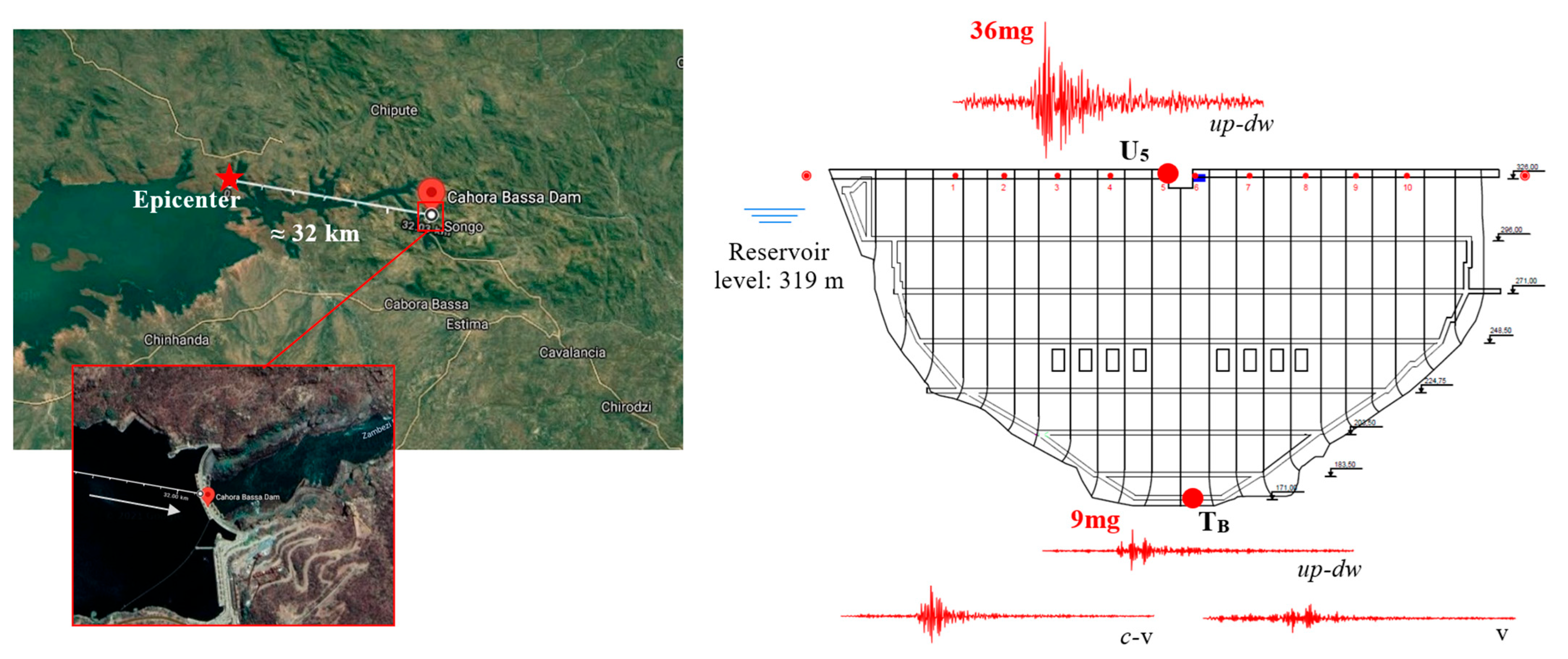
4.1. Case Study: Cahora Bassa Dam

The Cahora Bassa dam has been in operation since 1974 on the Zambezi River, near Songo, in the Western part of Mozambique (Figure 7). Built in a valley of granite rock mass of very good quality, the dam impounds Lake Cahora Bassa and is part of the largest hydroelectric scheme in southern Africa. Cahora Bassa is a 170 m high double curvature arch dam with a 303 m long crest, which was designed with a special half-hollow section. The central cantilever thickness ranges from 23 m at the base to 4 m at the top. The dam has a surface control spillway and eight half-height spillways. Under normal operating conditions, the reservoir level varies between el. 320 m and el. 326 m, that is from 11 to 5 m below the crest (at el. 331 m).

Regarding the dam’s structural condition, a concrete swelling phenomenon was detected during the 1980s, as evidenced by a typical cracking pattern on the crest surface. The analysis of the measured static response shows that the swelling process has been progressing over time; however, the evaluation of the modal parameters extracted from vibrations measured on the dam, using system identification methods and effect separation models, allowed for the conclusion that the modal response is mostly influenced by reservoir level variations [75], and thus, that dam performance is not being affected by the swelling.

In 2010, Hidroelétrica de Cahora Bassa (HCB) invested in the installation of a continuous vibration monitoring system for seismic and structural health monitoring (SSHM), aiming to improve dam safety control. This dynamic monitoring system, designed by the authors’ research group [76], was developed to enable a continuous assessment of dam performance in normal operating conditions, under ambient/operational vibrations, and to monitor the structural response during seismic events [16,75,77], providing valuable information to the dam owners and the engineers responsible for dam safety.

In what concerns the sensor layout (Figure 8), the system includes 13 force–balance accelerometers: 10 uniaxial sensors (EpiSensor ES-U2) installed along the upper gallery, 5 m below the crest, and 3 triaxial sensors (EpiSensor ES-T), with one located at the downstream base (inside the drainage gallery) and the other two in the right and left banks. All accelerometers were installed in suitable enclosures for protection and connected to a 24-channel Granite recorder for continuous data acquisition. The complete system was supplied by Kinemetrics. As for the software component, the system includes fully customized computational tools developed by the authors [78], notably for automatic data acquisition and management, as well as for modal parameter identification.

4.2. Numerical Model: Dam–Reservoir–Foundation System and Main Properties

The numerical simulations presented in this paper were performed using the reference finite element model for the Cahora Bassa dam–reservoir–foundation system shown in Figure 9. The dam mesh (1524 elements) accurately represents the dam geometry, including the half-hollow crest and the spillways. The mesh is comprised of cantilevers with three elements along the cross-section in order to better reproduce the stress variations along the thickness. The semi-infinite reservoir (2540 elements) extends to about 350 m beyond the upstream face of the dam, while the foundation block (616 elements) represents the rock mass around the dam, from the abutments to the base, with a maximum depth of about 100 m. Several tests were carried out to assess the mesh refinement. The mesh used herein allowed for achieving very good results in the modal analyses and seismic response simulations—as shown later in this paper—while also ensuring very satisfactory computation times.

As for the material properties, the dam concrete and foundation rock are taken to be isotropic materials with linear–elastic behavior, considering a Young’s modulus of E = 40 GPa and a Poisson’s ratio of v = 0.2. The concrete specific weight is γ = 24 kN/m³. The foundation is computed as an elastic massless substructure with damping (proportional to the foundation stiffness). A Rayleigh damping law was used for the dam, with a minimum value of about 1% (at the frequency of the first vibration mode). The reservoir water was hypothesized as a compressible fluid, assuming an average pressure wave propagation velocity (c_w) throughout the reservoir domain. In order to simulate the dynamic behavior of the Cahora Bassa dam, the material properties of the model were calibrated based on the experimental modal parameters extracted from vibrations measured during the initial monitoring years, between August 2010 and December 2013. Several comparative analyses were conducted using data gathered for different reservoir water levels to consider the response measured under conditions that are characteristic of the regular operating conditions of the Cahora Bassa dam [16]. The calibrated properties were the concrete and rock dynamic elasticity moduli, which were adjusted by applying a multiplicative factor C_E = 1.16 to the static values (the concrete elasticity modulus under dynamic loads can be measured directly using ultra-sound tests), and the value of the pressure waves’ propagation velocity, which in this case is c_w = 1585 m/s (a value consistent with the reservoir water temperature [16]).

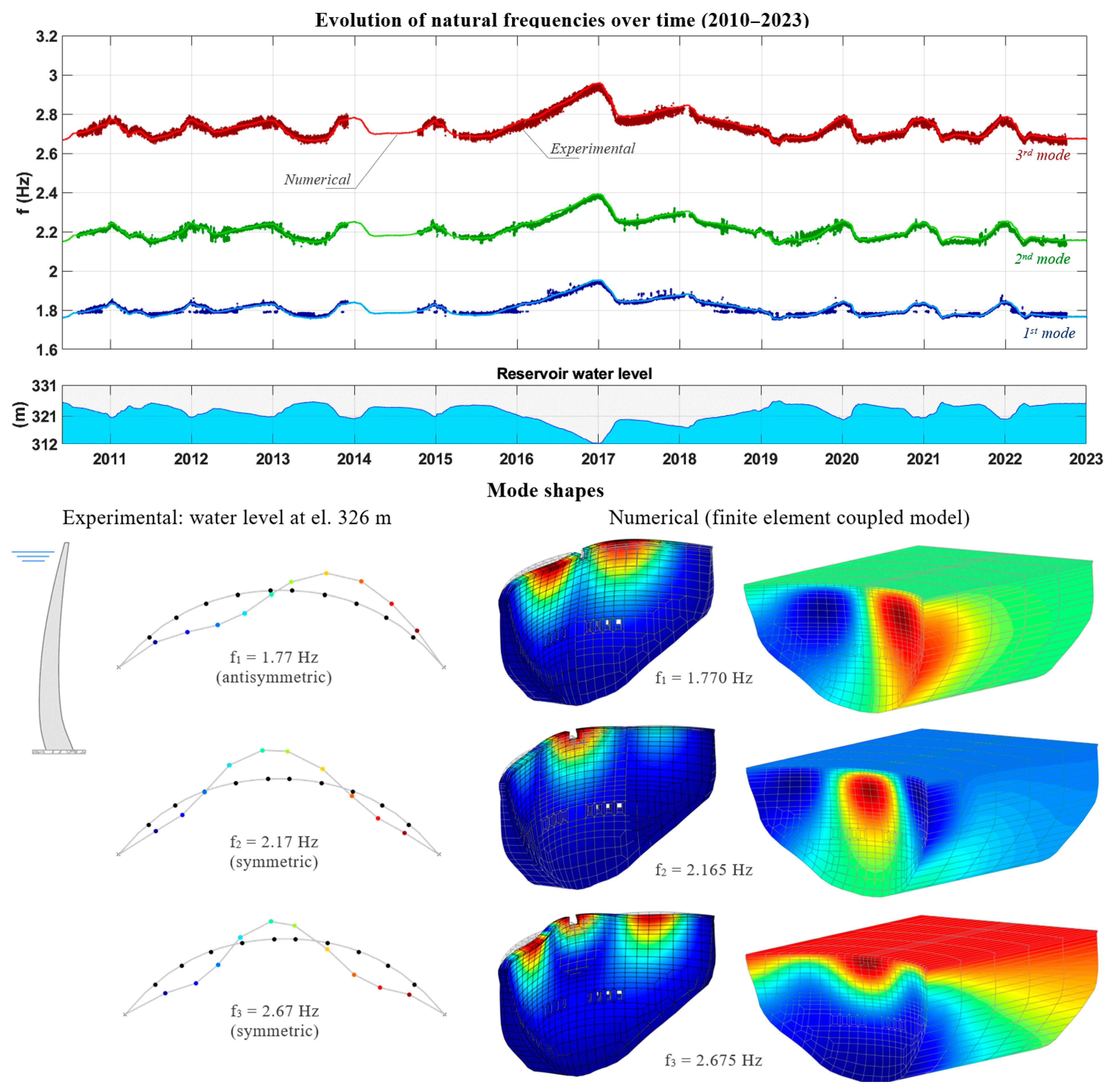
4.3. Modal Response: Natural Frequencies and Mode Shapes

This section presents a study on the modal response of the Cahora Bassa dam. Figure 10 shows the evolution of the natural frequencies over time, for the first three vibration modes, as well as the corresponding modal configurations for a scenario with the reservoir at el. 326 m (that is, 5 m below the crest level). The comparison is made between the experimental modal identification outputs and finite element results.

The identified frequencies and mode shapes were extracted from vibrations measured continuously on the dam under ambient/operational conditions, from August 2010 to December 2022, using an automated modal identification code based on the classic Frequency Domain Decomposition method [79,80], which is part of the dam’s monitoring system software [78]. It is worth noting that the system has been fully operational since its installation, except for a 10-month period between late 2014 and 2015. The numerical modal analyses were conducted based on the proposed state–space coupled formulation. The calibrated 3D finite element model for the Cahora Bassa dam–reservoir–foundation system (see Figure 9) was used to simulate the modal response, considering the measured reservoir water levels as inputs in the model.

With respect to the observed response of the dam, the variations in the experimental natural frequencies over time (colored dots in the graph) show that the reservoir level clearly influences the dynamic behavior of the dam–reservoir–foundation system: as the water level changes, so does the global mass of the system and, thus, the frequency values. It is also interesting to note how the variations in the frequency values are greater for the higher frequency modes. For example, the frequency of the first mode varies between 1.76 Hz, when the reservoir level is at its maximum, and 1.95 Hz, for the lowest water level, while for the third mode these values range between 2.67 Hz and 2.94 Hz.

The comparison with the finite element results shows that this behavior is effectively captured by the calibrated model for the dam–reservoir–foundation system over the entire monitoring period, i.e., for different reservoir conditions. This agrees with the findings of another study by the authors [75], which showed that it is the reservoir level’s effect that most affects the modal response of the Cahora Bassa dam, when compared with both the thermal effects (the temperature semi-amplitude at the dam site is around ±4 °C throughout the year) and the time effects.

As for the mode shapes, the first mode is antisymmetric, while the second and third modes are symmetric. In the case of this dam, these modal configurations are non-stationary and do not change for the existing reservoir conditions. The results of the finite element modal analysis, which gives the coupled dam–reservoir modes, show that the model can reproduce the mode shapes of all three vibration modes under analysis.

To sum up, the good agreement achieved between experimental and finite element results demonstrates that the modal response of the dam can be properly simulated by the calibrated model for the Cahora Bassa dam–reservoir–foundation system. Therefore, as initially intended, this study validates the coupled model and the proposed true coupled state–space approach, which instigated the formulation implemented in the finite element program DamDySSA5.0 for the modal analysis of dam–reservoir–foundation systems.

4.4. Seismic Response Under a Low-Intensity Earthquake

The seismic response of the Cahora Bassa dam is analyzed based on the accelerations measured with the dynamic monitoring system during a low-intensity seismic event detected at the dam site on 21 June 2017. Specifically, the accelerations recorded at the crest are compared with the response computed in a finite element linear seismic analysis.

The seismic event on 21 June 2017 occurred in Songo, about 32 km from the dam site, and the seismic waves arrived from the west–northwest, between the upstream–downstream and cross-valley directions. On that day, the water level in the reservoir was at el. 319 m, about 12 m below the crest level. Figure 11 shows the accelerograms recorded at the downstream base of the dam with the triaxial sensor T_B in the cross-valley (c-v), upstream–downstream (up-dw), and vertical (v) directions, as well as the acceleration time history measured near the crest of one of the central cantilevers, at about 5 m to the right of the central section, using the uniaxial accelerometer U₅. This was a near-field earthquake that induced low-amplitude vibrations in the dam structure. The recorded peak accelerations in the up–dw direction were 9 mg (milli-g) at the base and 36 mg at the top, which corresponds to a response amplification ratio of 4 times.

The finite element seismic analysis was conducted based on the proposed coupled time-stepping formulation, using the calibrated model for the dam–reservoir–foundation system. In order to consider realistic conditions in the seismic response simulation (Figure 12), the reservoir level in the model was set to 12 m below the crest, and the real seismic accelerations recorded at the downstream base of the dam were applied as seismic input (the simplified hypothesis of uniform ground motion is assumed). Furthermore, since the dam is subject to low amplitude vibrations, both the concrete and joint linear behavior are considered. Thus, the same Rayleigh damping law was used for the dam (a minimum value of about 1% at the frequency of the first vibration mode). These values are consistent with those used by other authors to reproduce the measured seismic response in large arch dams [18,19,20,81,82,83]. Despite the simplification adopted in the foundation and seismic input modeling, the comparison between the measured and computed accelerations shows that the calibrated model was able to reproduce the amplitude of the accelerations recorded at the crest of the dam in the up-dw direction quite well. Even with the simplified massless foundation model, the fact that the implemented formulation includes a damping component in the foundation (which is condensed, like the stiffness matrix, into the degrees of freedom in the dam–foundation interface) should help explain this good agreement. Similar conclusions were drawn in a study carried out by the authors for the Cabril arch dam. In this study, the results obtained with the model presented in this paper were successfully compared not only with measured accelerations during an earthquake on the dam but also with the seismic response, computed using software based on the mass foundation model [22]. To achieve a better agreement between the measured and computed seismic response of the dam, additional seismic measurements (along the dam base and in the free field) would be necessary to better characterize the seismic input.

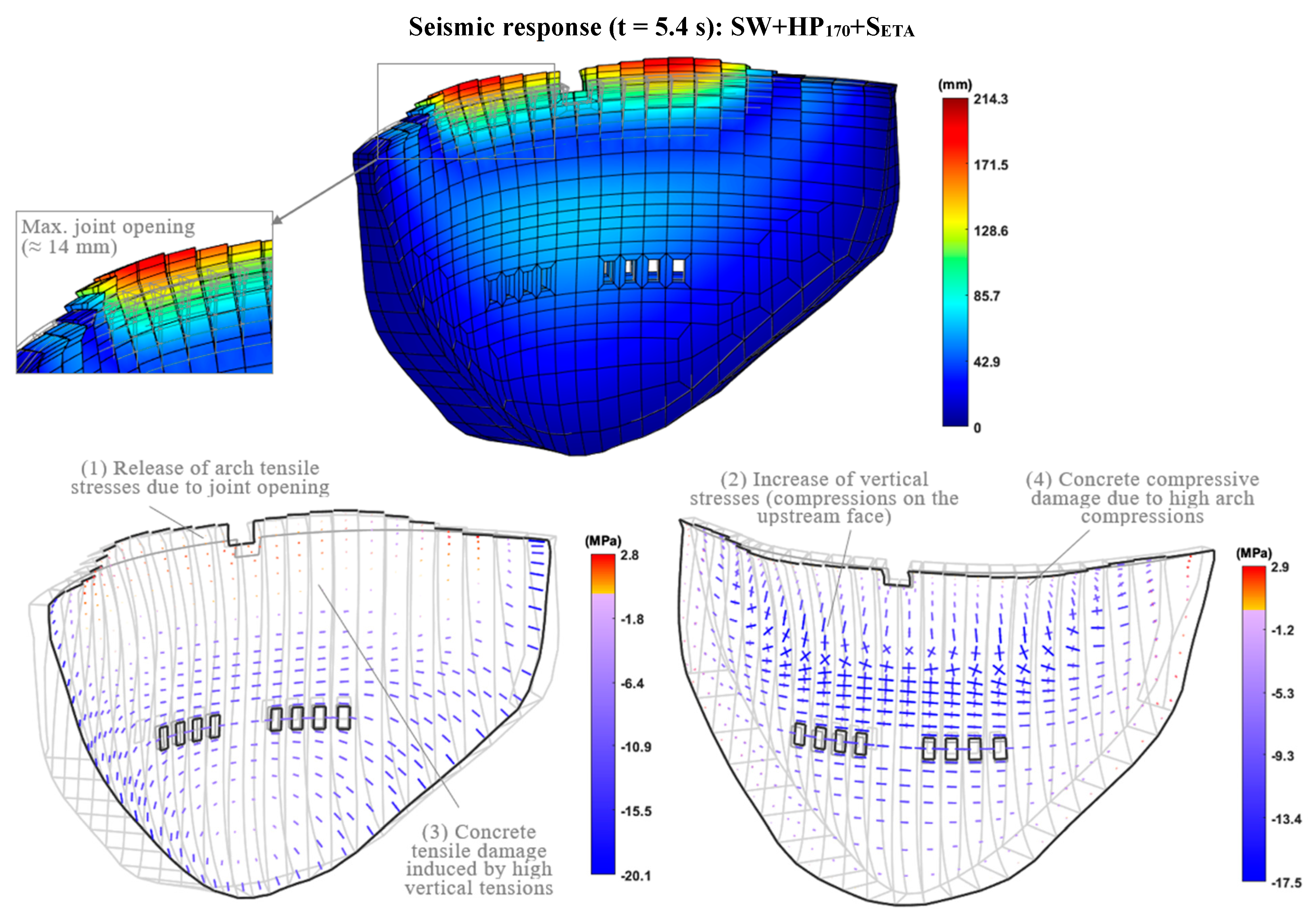
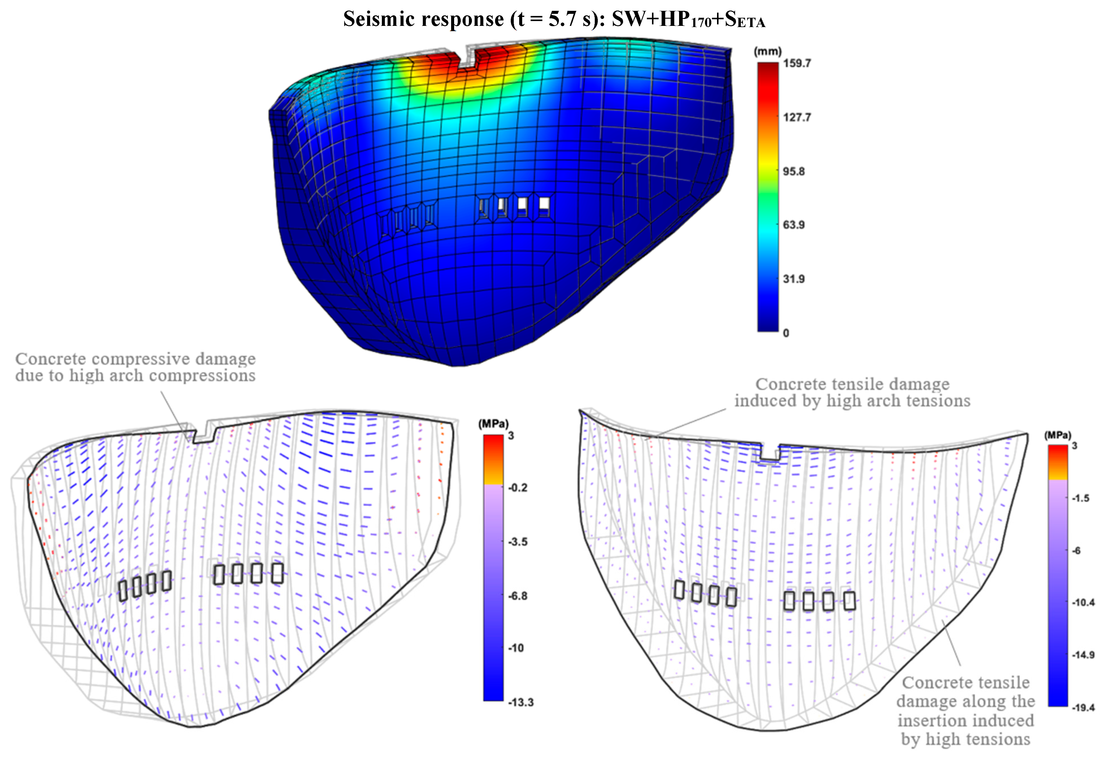
4.5. Nonlinear Seismic Analysis: Study on the Effects of Contraction Joint Movements and Concrete Damage

In the last application, an analysis of the nonlinear seismic behavior of the Cahora Bassa dam is presented. The goal is to assess the effects of the vertical joint movements on the structural response of the dam, and then to evaluate the evolution of tensile and compressive concrete damage. Therefore, the seismic computations were performed using the time-stepping formulation with stress–transfer, considering constitutive models for modeling the opening/closing and sliding movements of the vertical contraction joints and the behavior of concrete up to failure under tension and compression (see Section 3.4).

The nonlinear seismic response simulation was carried out for a load combination (Figure 13), including the self-weight of the dam (W), the hydrostatic pressure for a full reservoir scenario (HP₁₇₀), and the seismic action (S_ETA). The seismic input is given by an artificially designed intensifying acceleration time history [84], with the acceleration amplitude increasing to about 1 g in 10 s. This type of record is used for Endurance Time Analysis (ETA) [85].

The calibrated model for the dam–reservoir–foundation system was used for this seismic simulation. However, a total of 1269 interface elements were incorporated into the dam mesh to represent the vertical contraction joints. The joint properties are normal and the shear stiffness K_N = 5 × 10⁷ kNm⁻¹/m² and K_T = K_N/2, null cohesion c = 0, and friction angle ϕ = 30°. The joints’ damping matrices, proportional to the stiffness matrices, are computed using a coefficient β_J = 2.5 × 10⁻⁶. Additionally, the same constitutive damage law was adopted for all the dam elements to simulate the concrete’s nonlinear behavior. The main properties used are the tensile strength f_t = 3 MPa, fracture energy G_f = 0.9 kN.m/m², compressive strength f_c = −30 MPa, and ultimate compressive strain ${\epsilon }_u^{-}$ = −9.5 × 10⁻³. Damping ratios of 5% in the dam and 10% in the foundation are considered for the frequency band around the fundamental frequency.

The main results of the nonlinear seismic response of the dam under the load combination SW + HP₁₇₀ + S_ETA are presented in Figure 14, Figure 15 and Figure 16. First, the deformation of the dam and the corresponding principal stresses fields are analyzed for two instants of interest to show the effects of the vertical contraction joints on the structural response, specifically at t = 5.4 s, an instant when the dam suffers great deformations in the upstream direction, resulting in joint openings (Figure 14), and at t = 5.7 s, an instant characterized by important deformations in the downstream direction, presenting considerable compressive stresses (Figure 15). Afterwards, the evolution of both the tensile and compressive damage states is shown at different time steps (Figure 16).

Starting with the seismic response at t = 5.4 s (Figure 14), in this scenario, it is possible to see that the dam is pushed upstream by the seismic forces, with relative movements occurring between the lateral surfaces of the cantilevers due to the opening of the vertical contraction joints. The maximum upstream displacements (relative to the base), around 214 mm, occur at the top of the cantilevers located to the left and the right of the central zone. It is in these zones that the largest joint openings, approximately 14 mm, are computed. Regarding the principal stress fields, the results clearly show the effects caused by the vertical contraction joint movements. More specifically, the opening of the vertical joints reduces the arch effect, particularly at the upper blocks, resulting in the release of arch tensions near the top of the dam. In this way, tensile damage is avoided there. Nevertheless, this arch effect loss initiates a stress redistribution process that causes a gradual increase of vertical stresses along the height of the cantilevers, in particular, of the vertical tensions on the downstream face and vertical compressions on the upstream face. The vertical tensions on the downstream face of the dam end up exceeding the concrete tensile strength (3 MPa), and thus, concrete failure occurs along the upper half of the cantilevers (with damage values of up to 100%, as shown in Figure 16). Naturally, the tension values seen in the provided stress fields are lower than the concrete tensile strength, since the stresses above this value ended up being released due to the joint movements or causing concrete damage during the seismic simulation. Additionally, it is worth noting the high compressive stresses that arise along the downstream base of the dam (−15.5 to −20.1 MPa), oriented normally to the insertion line, as well as on the upstream surface, with compressions oriented both in the arch direction and vertically (−13.4 to −17.5 MPa).

At t = 5.7 s (Figure 15), the computed seismic response indicates that when the dam moves in the downstream direction, maximum displacements of about 160 mm occur at the top of the central cantilevers, near the surface spillway. In this case, the vertical contraction joints close, and the dam becomes mainly subject to compressive forces, as expected. The principal stress field reveals important arch compressions developing at the top of the central cantilevers of the dam, on the upstream face (−15 to −19.4 MPa). Since these compressions remain below the assumed compressive strength (−30 MPa), no compressive damage occurs in this central area. However, significant compressions are installed around the surface spillway, on the downstream surface, causing high compressive damage (with values close to 100%). In this scenario, it is also worth emphasizing that the dam deformation induces high tensions at the upstream base of the dam cantilevers, along almost the entire insertion, as well as high arch tensions in the upper area of the lateral cantilevers, as these are forced in the opposite direction to the central cantilevers. Therefore, these areas present high tensile damage values that cause concrete tensile failure (cracking).

Finally, the concrete damage results (Figure 16) allow for the evaluation of the progression of both tensile and compressive damage in the dam body during the seismic simulation. Since this seismic analysis was conducted using an artificial seismic action of increasing intensity, which can be applied for seismic safety assessment studies [86,87,88], the achieved results give clear indications on the seismic performance of the Cahora Bassa dam, enabling the detection of zones that are potentially susceptible under strong earthquakes.

With respect to the tensile damage evolution, the results are presented here up to t = 5 s (a ≈ 0.5 g). First, it is worth noting that tensile damage occurs along the upstream base, even for lower peak accelerations (up to 0.1 g). This was expected because in the Cahora Bassa dam, the combined action of the self-weight and the hydrostatic pressure (high water level) causes significant vertical tensions at the upstream base of the dam. Under higher seismic excitation levels, the tensile damage continues developing along the upstream base, and additional damage starts to arise at the upper blocks of the lateral cantilevers, on the downstream surface, with concrete failure occurring in some points. This is caused by the vertical tensions which, as mentioned before, derive from the stress redistribution process induced by the joint opening and the subsequent arch effect loss. Finally, for peak ground accelerations around 0.5 g, there is a clear aggravation of the damage state of the dam, with a significant propagation of concrete tensile failure along the upper half of the dam body due to the high vertical tensions that develop along the height of the cantilevers on the downstream side. Furthermore, concrete cracking also occurs on the upper blocks of the lateral cantilevers, on the upstream side, caused by the arch tensions that arise when the dam deforms in the downstream direction. Nevertheless, it is interesting to note that concrete cracking is mostly superficial, without propagation across the thickness of the cantilevers.

As for the evolution of compressive damage, until t = 5 s, there are no significant signs of damage resulting from compressions on the dam body, and only small damage values can be seen at the top of the upstream face of the lateral cantilevers (around 35%) and below the surface spillway (about 15%). After that, however, the compressive damage starts to gradually increase and spread around these zones, with compressive failure (concrete crushing) even occurring in some areas, particularly near the crest of the lateral cantilevers, on the upstream side, and at the top of the central cantilevers, to the side of the surface spillway, on the downstream surface.

The results achieved in this study on the seismic response of the Cahora Bassa dam under a strong and intensifying seismic action make it possible to emphasize the potential of the developed time-stepping formulation for the nonlinear seismic analysis of dam–reservoir–foundation systems, considering both joint and material nonlinear behavior. Specifically, the effects on the structural response caused by the vertical joint movements were according to expectations, while the computed tensile and compressive damage states were consistent with the resulting principal stress fields.

Finally, it is important to note that the dam is located in a low seismic risk zone. The peak ground acceleration values of 0.076 g for the Operating Basis Earthquake (OBE) and 0.102 g for the Maximum Design Earthquake (MDE) were defined in a seismic hazard study for the dam site. Therefore, using the presented nonlinear model for the Cahora Bassa dam, it is possible to show that the dam exhibits a very good seismic performance: severe tensile damage (cracking across the entire section) does not occur for accelerations up to 0.5 g (around 6.5 times the OBE) and significant compressive damage (crushing at the top of the central blocks) does not occur under accelerations up to 0.8 g (about 8 times the MDE).

5. Discussion

This paper presented a finite element formulation for the dynamic analysis of dam–reservoir–foundation systems, based on a new coupled approach that uses a single global unknown vector combining both displacements and pressures.

While the classical approach adopted for coupled models involves separating the solid and fluid equations and then symmetrizing the problem, this work proposed a true coupled approach that originates a non-symmetrical finite element equation, describing the dynamic behavior of the global dam–reservoir–foundation system with generalized damping. Using this new approach, the dynamic equation is solved directly to compute the response in displacements and hydrodynamic pressures, considering radiation damping in the reservoir and assuming the hypothesis of non-proportional damping in the dam body and/or the foundation. This is an important advantage as it allows for the simulation of the behavior of dams with different materials and/or deteriorated zones, with low stiffness and higher damping.

Additionally, new formulations were presented to solve the coupled finite element equation, specifically for complex modal analysis and for simulating the linear and nonlinear response under seismic forces.

When it comes to modal analysis, an innovative state–space formulation has been developed to compute the vibration modes of the entire solid–fluid system by solving a non-symmetrical eigenproblem with damping, which results in complex eigenvalues and eigenvectors. Physically, these correspond to non-stationary vibration modes, a type of mode shape that has been experimentally identified from vibrations measured on some large concrete dams.

For seismic response analysis, a simple time-stepping formulation is proposed, based on the application of the Newmark method to the coupled dynamic equation discretized in time. This formulation enables the joint calculation of the displacements (dam–foundation) and pressures (reservoir) of the discretized system in the time domain.

Regarding nonlinear seismic analysis, a time-stepping formulation combined with a stress–transfer method has been developed, using suitable constitutive models to simulate both the effects due to joint movements and the concrete damage. Specifically, at each time step, the stress–transfer process sequentially redistributes the unbalanced stresses: first, due to nonlinear joint behavior, and second, due to concrete failure. This is achieved using (a) a joint constitutive model based on the Mohr–Coulomb failure criterion and on appropriate stress–displacement laws, to simulate opening/closing and sliding joint movements, and (b) a concrete constitutive model with softening and two independent scalar damage variables, to simulate both tensile and compressive damage.

Finally, this paper has also provided the results from the latest application studies conducted in the case of the Cahora Bassa dam, including experimental results obtained using data from the continuous vibrations monitoring system (installed in 2010) and numerical results obtained using the developed program (DamDySSA5.0).

First, the modal response of the dam was analyzed. The identified natural frequencies (time evolution over a decade, from 2010 to 2023, for different reservoir water levels) and the modal configurations for the first three vibration modes were compared with finite element results, computed using a calibrated model for the Cahora Bassa dam–reservoir–foundation system. A very good agreement was achieved between the modal identification outputs and the finite element results.

Next, the seismic response of the dam was analyzed for a low magnitude near-field seismic event that was measured at the dam site on 21 June 2017. The accelerations recorded at the crest were compared against finite element results achieved in a linear seismic simulation. Overall, it was possible to reproduce the response in terms of the acceleration amplitudes at the dam crest, using the accelerations recorded at the dam base as the seismic input (uniform ground motion), the real water level in the reservoir model, and assuming consistent damping values (1% in the dam and 5% in the foundation). For future studies, additional measurements along the dam base and in the free field will be necessary in order to better characterize the seismic input and, consequently, to achieve a better agreement between the measured and computed seismic response of the dam.

After that, a complete seismic response analysis was presented, considering a full reservoir scenario and applying an intensifying seismic action (increasing acceleration amplitudes). As expected for an arch dam, the achieved results mainly showed that (a) when the dam moves upstream, the opening of the vertical contraction joints causes a release in the arch stresses along the upper blocks, resulting in a stress redistribution that leads to the installation of greater vertical tensions along the height of the cantilevers, which ultimately originates concrete tensile failure (cracking), and (b) as the dam bends in the downstream direction, the vertical joints close and there is an overall increase in the compressions’ values along the arches on the upper part of the dam, which can potentially lead to compressive damage and, in more severe cases, to compressive failure (concrete crushing).

6. Conclusions

This work provides an important contribution at the level of the numerical modeling of the dynamic behavior of concrete dams by presenting a robust yet simple formulation, with several innovative aspects for the modal analysis and nonlinear seismic modeling of dam–reservoir-–oundation systems. The results achieved in the application studies for a real large arch dam showed the suitability and robustness of the proposed coupled approach, as well as the potential of the developed formulation for simulating the modal response and linear and nonlinear seismic behavior simulations.

The coupled model and proposed formulation were implemented in the latest version of the computer program DamDySSA5.0, which has been under development by the authors for several years. This program has become an essential tool, used by students and engineers to carry out studies for simulating the observed response of dams under ambient/operational conditions and for modeling the structural response under seismic actions. Additionally, the program has provided valuable results to support structural health and performance monitoring, and it has been employed to carry out behavior prediction studies, including for the seismic safety assessment of large concrete dams.

In addition, this paper also offers a relevant contribution by providing important experimental results in the case of Cahora Bassa, which has been instrumented since 2010 with a continuous vibration monitoring system (one of the first in the world). Specifically, the Operational Modal Analysis results, obtained from over a decade of vibration data, are unique and offer a reliable benchmark case for researchers and engineers working in the field of dam dynamics and structural health monitoring.

References

1. Chopra, A.K. Earthquake Analysis of Arch Dams: Factors to Be Considered. J. Struct. Eng. 2012, 138, 205–214. [Google Scholar] [CrossRef]
2. Chen, H. Seismic Safety of High Concrete Dams. Earthq. Eng. Eng. Vib. 2014, 13, 1–16. [Google Scholar] [CrossRef]
3. Fenves, G.L.; Chopra, A.K. Effects of Reservoir Bottom Absorption on Earthquake Response of Concrete Gravity Dams. Earthq. Eng. Struct. Dyn. 1983, 11, 809–829. [Google Scholar] [CrossRef]
4. Pedro, J.O.; Câmara, R. Coupled Models for Dynamic Analysis of Arch Dams. In Proceedings of the 8th European Conference on Earthquake Engineering, LNEC, Lisbon, Portugal, 7–12 September 1986. [Google Scholar]
5. Fok, K.L.; Chopra, A.K. Earthquake Analysis of Arch Dams Including Dam-Water Interaction, Reservoir Boundary Absorption and Foundation Flexibility. Earthq. Eng. Struct. Dyn. 1986, 14, 155–184. [Google Scholar] [CrossRef]
6. Tiliouine, B.; Seghir, A. Fluid-Structure Models for Dynamic Studies of Dam-Water Systems. In Proceedings of the 11th European Conference on Earthquake Engineering, Paris, France, 6–11 September 1998. [Google Scholar]
7. Küçükarslan, S.; Coşkun, S.B.; Taşkın, B. Transient Analysis of Dam–Reservoir Interaction Including the Reservoir Bottom Effects. J. Fluids Struct. 2005, 20, 1073–1084. [Google Scholar] [CrossRef]
8. Bouaanani, N.; Lu, F.Y. Assessment of Potential-Based Fluid Finite Elements for Seismic Analysis of Dam-Reservoir Systems. Comput. Struct. 2009, 87, 206–224. [Google Scholar] [CrossRef]
9. Zhang, C.; Pan, J.; Wang, J.-T. Influence of Seismic Input Mechanisms and Radiation Damping on Arch Dam Response. Soil Dyn. Earthq. Eng. 2009, 29, 1282–1293. [Google Scholar] [CrossRef]
10. Oliveira, S.; Silvestre, A.; Espada, M.; Câmara, R. Modeling the Dynamic Behavior of Dam-Reservoir-Foundation Systems Considering Generalized Damping. Development of a 3DFEM State Formulation. In Proceedings of the International Conference on Structural Dynamic EURODYN, Porto, Portugal, 30 June–2 July 2014. [Google Scholar]
11. Lokke, A.; Chopra, A.K. Direct Finite Element Method for Nonlinear Earthquake Analysis of 3-Dimensional Semi-Unbounded Dam–Water-Foundation Rock Systems. Earthq. Eng. Struct. Dyn. 2018, 47, 1309–1328. [Google Scholar] [CrossRef]
12. Daniell, W.E.; Taylor, C.A. Effective Ambient Vibration Testing for Validating Numerical Models of Concrete Dams. Earthq. Eng. Struct. Dyn. 1999, 28, 1327–1344. [Google Scholar] [CrossRef]
13. Darbre, G.R.; de Smet, C.A.M.; Kraemer, C. Natural Frequencies Measured from Ambient Vibration Response of the Arch Dam of Mauvoisin. Earthq. Eng. Struct. Dyn. 2000, 29, 577–586. [Google Scholar] [CrossRef]
14. Proulx, J.; Paultre, P.; Rheault, J.; Robert, Y. An Experimental Investigation of Water Level Effects on the Dynamic Behaviour of a Large Arch Dam. Earthq. Eng. Struct. Dyn. 2001, 30, 1147–1166. [Google Scholar] [CrossRef]
15. Sevim, B.; Bayraktar, A.; Altunışık, A.C.; Adanur, S.; Akköse, M. Determination of Water Level Effects on the Dynamic Characteristics of a Prototype Arch Dam Model Using Ambient Vibration Testing. Exp. Tech. 2012, 36, 72–82. [Google Scholar] [CrossRef]
16. Alegre, A.; Carvalho, E.; Matsinhe, B.; Mendes, P.; Oliveira, S.; Proença, J. Monitoring Vibrations in Large Dams. In Proceedings of the HYDRO 2019—Concept to Closure: Practical Steps, Porto, Portugal, 14–16 October 2019. [Google Scholar]
17. Guo, X.; Dufour, F.; Humbert, N. Modal Analysis of an Arch Dam Combining Ambient Vibration Measurements, Advanced Fluid-element Method and Modified Engineering Approach. Earthq. Eng. Struct. Dyn. 2022, 51, 1321–1342. [Google Scholar] [CrossRef]
18. Proulx, J.; Darbre, G.R. Earthquake Response of Large Arch Dams. Observational Evidence and Numerical Modelling. In Proceedings of the 14th World Conference on Earthquake Engineering, Beijing, China, 12–17 October 2008. [Google Scholar]
19. Chopra, A.K.; Wang, J.-T. Earthquake Response of Arch Dams to Spatially Varying Ground Motion. Earthq. Eng. Struct. Dyn. 2010, 39, 887–906. [Google Scholar] [CrossRef]
20. Robbe, E.; Kashiwayanagi, M.; Yamane, Y. Seismic Analyses of Concrete Dam, Comparison between Finite-Element Analyses and Seismic Records. In Proceedings of the 16th World Conference on Earthquake Engineering, Santiago, Chile, 9–17 January 2017. [Google Scholar]
21. Koufoudi, E.; Chaljub, E.; Dufour, F.; Bard, P.Y.; Humbert, N.; Robbe, E. Spatial Variability of Earthquake Ground Motions at the Dam–Foundation Rock Interface of Saint Guérin: Experimental and Numerical Investigations. Bull. Earthq. Eng. 2018, 16, 1751–1777. [Google Scholar] [CrossRef]
22. Alegre, A.; Robbe, E.; Oliveira, S. Seismic Analysis of Cabril Dam. Measured Response and Comparison with Numerical Results from Code_Aster and DamDySSA. In Proceedings of the 4th Dam World Conference, LNEC, Lisboa, Portugal, 22–24 September 2020. [Google Scholar]
23. Oliveira, S.; Alegre, A.; Carvalho, E.; Mendes, P.; Proença, J. Seismic and Structural Health Monitoring Systems for Large Dams: Theoretical, Computational and Practical Innovations. Bull. Earthq. Eng. 2022, 20, 4483–4512. [Google Scholar] [CrossRef]
24. Wang, J.-T.; Zhang, C.; Jin, F. Nonlinear Earthquake Analysis of High Arch Dam-Water-Foundation Rock Systems. Earthq. Eng. Struct. Dyn. 2012, 41, 1157–1176. [Google Scholar] [CrossRef]
25. Hariri-Ardebili, M.A.; Mirzabozorg, H. Seismic Performance Evaluation and Analysis of Major Arch Dams Considering Material and Joint Nonlinearity Effects. ISRN Civ. Eng. 2012, 2012, 681350. [Google Scholar] [CrossRef]
26. Hariri-Ardebili, M.A.; Mirzabozorg, H.; Estekanchi, H.E. Nonlinear Seismic Assessment of Arch Dams and Investigation of Joint Behavior Using Endurance Time Analysis Method. Arab. J. Sci. Eng. 2014, 39, 3599–3615. [Google Scholar] [CrossRef]
27. Goldgruber, M. Non-Linear Seismic Modelling of Concrete Dams. Ph.D. Thesis, Graz University of Technology, Graz, Austria, 2015. [Google Scholar]
28. Wang, R.; Chen, L.; Zhang, C. Seismic Design of Xiluodu Ultra-High Arch Dam. Water Sci. Eng. 2018, 11, 288–301. [Google Scholar] [CrossRef]
29. Alegre, A. Modelling and Monitoring the Dynamic Behaviour of Concrete Dams. Modal Analysis and Seismic Response. Ph.D. Thesis, Instituto Superior Técnico, University of Lisbon, Lisbon, Portugal, 2021. [Google Scholar]
30. Niwa, A.; Clough, R.W. Non-Linear Seismic Response of Arch Dams. Earthq. Eng. Struct. Dyn. 1982, 10, 267–281. [Google Scholar] [CrossRef]
31. Fenves, G.L.; Mojtahedi, S.; Reimer, R.B. Effect of Contraction Joints on Earthquake Response of an Arch Dam. J. Struct. Eng. 1992, 118, 1039–1055. [Google Scholar] [CrossRef]
32. Lau, D.T.; Boruziaan, B.; Razaqpur, A.G. Modelling of Contraction Joint and Shear Sliding Effects on Earthquake Response of Arch Dams. Earthq. Eng. Struct. Dyn. 1998, 27, 1013–1029. [Google Scholar] [CrossRef]
33. Câmara, R. A Method for Coupled Arch Dam-Foundation-Reservoir Seismic Behaviour Analysis. Earthq. Eng. Struct. Dyn. 2000, 29, 441–460. [Google Scholar] [CrossRef]
34. Faria, R.; Oliver, J.; Cervera, M. A Strain-Based Plastic Viscous-Damage Model for Massive Concrete Structures. Int. J. Solids Struct. 1998, 35, 1533–1558. [Google Scholar] [CrossRef]
35. Valliappan, S.; Yazdchi, M.; Khalili, N. Seismic Analysis of Arch Dams—A Continuum Damage Mechanics Approach. Int. J. Numer. Methods Eng. 1999, 45, 1695–1724. [Google Scholar] [CrossRef]
36. Oliveira, S.; Faria, R. Numerical Simulation of Collapse Scenarios in Reduced Scale Tests of Arch Dams. Eng. Struct. 2006, 28, 1430–1439. [Google Scholar] [CrossRef]
37. Pan, J.; Zhang, C.; Xu, Y.; Jin, F. A Comparative Study of the Different Procedures for Seismic Cracking Analysis of Concrete Dams. Soil Dyn. Earthq. Eng. 2011, 31, 1594–1606. [Google Scholar] [CrossRef]
38. Omidi, O.; Lotfi, V. Earthquake Response of Concrete Arch Dams: A Plastic–Damage Approach. Earthq. Eng. Struct. Dyn. 2013, 42, 2129–2149. [Google Scholar] [CrossRef]
39. Westergaard, H.M. Water Pressures on Dams during Earthquakes. Trans. Am. Soc. Civ. Eng. 1933, 98, 418–472. [Google Scholar] [CrossRef]
40. Kuo, J.S.H. Fluid-Structure Interactions: Added Mass Computations for Incompressible Fluid; Report No. UCB/EERC-82/09; University of California: Berkeley, CA, USA, 1982. [Google Scholar]
41. Miquel, B.; Bouaanani, N. Simplified Evaluation of the Vibration Period and Seismic Response of Gravity Dam–Water Systems. Eng. Struct. 2010, 32, 2488–2502. [Google Scholar] [CrossRef]
42. Altunisik, A.C.; Sesli, H. Dynamic Response of Concrete Gravity Dams Using Different Water Modelling Approaches: Westergaard, Lagrange and Euler. Comput. Concr. 2015, 16, 429–448. [Google Scholar] [CrossRef]
43. Xu, H.; Zou, D.; Kong, X.; Su, X. Error Study of Westergaard’s Approximation in Seismic Analysis of High Concrete-Faced Rockfill Dams Based on SBFEM. Soil Dyn. Earthq. Eng. 2017, 94, 88–91. [Google Scholar] [CrossRef]
44. Wang, M.; Chen, J.; Wu, L.; Song, B. Hydrodynamic Pressure on Gravity Dams with Different Heights and the Westergaard Correction Formula. Int. J. Geomech. 2018, 18, 04018134. [Google Scholar] [CrossRef]
45. Zienkiewicz, O.C.; Bettess, P. Fluid-Structure Dynamic Interaction and Wave ForcesAn Introduction to Numerical Treatment. Int. J. Numer. Methods Eng. 1978, 13, 1–16. [Google Scholar] [CrossRef]
46. Sani, A.A.; Lotfi, V. Dynamic Analysis of Concrete Arch Dams by Ideal-Coupled Modal Approach. Eng. Struct. 2010, 32, 1377–1383. [Google Scholar] [CrossRef]
47. Oliveira, S.; Alegre, A.; Silvestre, A.; Espada, M.; Câmara, R. Seismic Safety Evaluation of Luzzone Dam. Use of a 3DFEM State Formulation in Pressures and Displacements. In Proceedings of the 13th ICOLD International Benchmark Workshop on Numerical Analysis of Dams, Lausanne, Switzerland, 9–11 September 2015. [Google Scholar]
48. Zienkiewicz, O.C.; Taylor, R.L.; Zhu, J.Z. The Finite Element Method: Its Basis and Fundamentals, 7th ed.; Elsevier Butterworth-Heinemann: Oxford, UK, 2013. [Google Scholar]
49. Ohayon, R. Symmetric Variational Formulations for Harmonic Vibration Problems Coupling Primal and Dual Variables—Application to Fluid-Structure Coupled Systems. La Rechereche Aerosp. 1979, 3, 69–77. [Google Scholar]
50. Daniel, W.J. Modal Methods in Finite Element Fluid-Structure Problems with Mixed Variables. Int. J. Numer. Methods Eng. 1980, 15, 1161–1175. [Google Scholar] [CrossRef]
51. Ohayon, R.; Valid, R. True Symmetric Formulation of Free Vibrations for Fluid-Structure Interaction in Bounded Media—Finite Element Results. In Numerical Methods in Coupled Systems; Lewis, R.W., Bettess, P., Hinton, E., Eds.; John Wiley & Sons: Hoboken, NJ, USA, 1984. [Google Scholar]
52. Felippa, C.A. Symmetrization of Coupled Eigenproblems by Eigenvector Augmentation. Commun. Appl. Numer. Methods 1988, 4, 561–563. [Google Scholar] [CrossRef]
53. Lotfi, V. Frequency Domain Analysis of Concrete Arch Dams by Decoupled Modal Approach. Struct. Eng. Mech. 2005, 21, 423–435. [Google Scholar] [CrossRef]
54. Zienkiewicz, O.C.; Taylor, R.L. Coupled Problems—A Simple Time-Stepping Procedure. Commun. Appl. Numer. Methods 1985, 1, 233–239. [Google Scholar] [CrossRef]
55. Veletsos, A.; Ventura, C. Modal Analysis of Non-Classically Damped Linear Systems. Earthq. Eng. Struct. Dyn. 1986, 14, 217–243. [Google Scholar] [CrossRef]
56. Oliveira, S.; Alegre, A. Vibrations in Large Dams. Monitoring and Modelling. In Proceedings of the 26th ICOLD Congress on Large Dams, Vienna, Austria, 1–7 July 2018. [Google Scholar]
57. Alegre, A.; Oliveira, S.; Espada, M.; Câmara, R.; Lemos, J. Hydrodynamic Pressures on Dams. Numerical and Experimental Results for Non-Vertical Upstream Faces. In Proceedings of the 10 °Congresso Nacional de Mecânica Experimental, LNEC, Lisboa, Portugal, 12–14 October 2016. [Google Scholar]
58. Oliveira, S.; Alegre, A. Seismic and Structural Health Monitoring of Dams in Portugal. In Seismic Structural Health Monitoring; Limongelli, M.P., Çelebi, M., Eds.; Springer Tracts in Civil Engineering; Springer International Publishing: Cham, Switzerland, 2019; pp. 87–113. ISBN 978-3-030-13975-9. [Google Scholar]
59. Newmark, N. A Method of Computation for Structural Dynamics. J. Eng. Mech. Div. 1959, 85, 67–94. [Google Scholar] [CrossRef]
60. Alegre, A.; Oliveira, S. Non-Linear Seismic Analysis of Arch Dams Considering Joint Movements and a Concrete Damage Model. In Proceedings of the 4th Dam World Conference, LNEC, Lisboa, Portugal, 21–25 September 2020. [Google Scholar]
61. Clough, R.W.; Penzien, J. Dynamics of Structures, 3rd ed.; Computers & Structures, Inc: Berkeley, CA, USA, 2003. [Google Scholar]
62. de Borst, R.; Sluys, L.J. Computational Methods in Non-Linear Solid Mechanics; Faculty of Civil Engineering and Geosciences, Delft University of Technology: Delft, The Netherlands, 1999. [Google Scholar]
63. Zienkiewicz, O.C.; Taylor, R.L.; Fox, D.D. The Finite Element Method for Solid and Structural Mechanics, 7th ed.; Elsevier: Amsterdam, The Netherlands, 2014; ISBN 9781856176347. [Google Scholar]
64. Alegre, A.; Oliveira, S.; Mendes, P.; Proença, J.; Carvalho, E.; Matsinhe, B. Numerical Models for Seismic Analysis of Arch Dams. In Proceedings of the Congreso de Métodos Numéricos en Ingeniería (CMNE2022), Las Palmas de Gran Canaria, Spain, 12–14 September 2022; pp. 411–430. [Google Scholar]
65. Alegre, A.; Oliveira, S.; Mendes, P.; Proença, J.; Ramos, R.; Carvalho, E. Seismic Safety Assessment of Arch Dams Using an ETA-Based Method with Control of Tensile and Compressive Damage. Water 2022, 14, 3835. [Google Scholar] [CrossRef]
66. Lemaitre, J. How to Use Damage Mechanics. Nucl. Eng. Des. 1984, 80, 233–245. [Google Scholar] [CrossRef]
67. Simo, J.C.; Ju, J.W. Strain- and Stress-Based Continuum Damage Models—I. Formulation. Int. J. Solids Struct. 1987, 23, 821–840. [Google Scholar] [CrossRef]
68. Simo, J.C.; Ju, J.W. Strain- and Stress-Based Continuum Damage Models—II. Computational Aspects. Int. J. Solids Struct. 1987, 23, 841–869. [Google Scholar] [CrossRef]
69. Faria, R.; Oliver, J. A Rate-Dependent Plastic-Damage Constitutive Model for Large Scale Computations in Concrete Structures. Monogr. Cent. Int. Metod. Numer. Ing. 1993, 17, 78. [Google Scholar]
70. Bažant, Z.P.; Oh, B.H. Crack Band Theory for Fracture of Concrete. Mater. Struct. 1983, 16, 155–177. [Google Scholar] [CrossRef]
71. Clough, R.W. Non-Linear Mechanisms in the Seismic Response of Arch Dams. In Proceedings of the International Research Conference on Earthquake Engineering, Skopje, Yugoslavia, 30 June–3 July 1980. [Google Scholar]
72. Fenves, G.L.; Mojtahedi, S.; Reimer, R.B. ADAP-88: A Computer Program for Non-Linear Earthquake Analysis of Concrete Arch Dams; University of California: Berkeley, CA, USA, 1989. [Google Scholar]
73. Fok, K.L.; Hall, J.F.; Chopra, A.K. EACD-3D: A Computer Program for Three-Dimensional Earthquake Analysis of Concrete Dams; University of California: Berkeley, CA, USA, 1986. [Google Scholar]
74. Zangar, C.N. Hydrodynamic Pressures on Dams Due to Horizontal Earthquake Effects; Engineering Monograph, No. 11; Bureau of Reclamation: Washington, DC, USA, 1952.
75. Oliveira, S.; Mendes, P.; Rodrigues, M.; Alegre, A.; Proença, J.; Carvalho, E.; Matsinhe, B. Cahora Bassa Vibrations Monitoring between 2010–2022. Analysis of Frequencies Using HST Statistical Models for Effects Separation. In Proceedings of the XII International Conference on Structural Dynamics (EURODYN 2023), TU Delft, Delft, The Netherlands, 2–5 July 2023. [Google Scholar]
76. Carvalho, E.; Matsinhe, B. First Steps on Automatic Data Acquisition and Analysis System in Cahora Bassa Dam. In Proceedings of the HYDRO 2014, Como, Italy, 13–15 October 2014. [Google Scholar]
77. Alegre, A.; Mendes, P.; Carvalho, E.; Matsinhe, B.; Oliveira, S.; Proença, J. Use of SSHM Data for Dynamic Behavior Analysis and Damage Detection on Large Dams. The Cases of Cabril Dam and Cahora Bassa Dam. In Proceedings of the 10th International Conference on Structural Health Monitoring of Intelligent Infrastructure (SHMII-10), Porto, Portugal, 30 June–2 July 2021; Álvaro, C., Caetano, E., Eds.; International Society for Structural Health Monitoring of Intelligent Infrastructure (ISHMII): Winnipeg, MB, Canada, 2021. [Google Scholar]
78. Carvalho, E.; Matsinhe, B.; Mendes, P.; Oliveira, S.; Alegre, A.; Ciudad-Real, M.; Skolnik, D.; El-Idrissi, M. SSHM Systems for Dams: 12 Years’ Experience in Cahora Bassa Dam. Equipment, Software, and Main Results. In Experimental Vibration Analysis for Civil Engineering Structures (EVACES 2023); Limongelli, M.P., Giordano, P.F., Quqa, S., Gentile, C., Cigada, A., Eds.; Lecture Notes in Civil Engineering; Springer: Cham, Switzerland, 2023; pp. 273–282. [Google Scholar]
79. Brincker, R.; Zhang, L.; Andersen, P. Modal Identification from Ambient Responses Using Frequency Domain Decomposition. In Proceedings of the IMAC18: International Modal Analysis Conference, San Antonio, TX, USA, 7–10 February 2000. [Google Scholar]
80. Peeters, B. System Identification and Damage Detection in Civil Engineering. Ph.D. Thesis, Faculteit Toegepaste Wetenschapen, Katholieke Universiteir Leuven, Leuven, Belgium, 2000. [Google Scholar]
81. Proulx, J.; Darbre, G.R.; Kamileris, N. Analytical and Experimental Investigation of Damping in Arch Dams Based on Recorded Earthquakes. In Proceedings of the 13th World Conference on Earthquake Engineering, Vancouver, BC, Canada, 1–6 August 2004. [Google Scholar]
82. Wang, J.-T.; Chopra, A.K. Linear Analysis of Concrete Arch Dams Including Dam-Water-Foundation Rock Interaction Considering Spatially Varying Ground Motions. Earthq. Eng. Struct. Dyn. 2010, 39, 731–750. [Google Scholar] [CrossRef]
83. Robbe, E. Seismic Back Analysis of Monticello Arch Dam—Blind Prediction Workshop and Additional Analyses. In Proceedings of the USSD 2017 Annual Conference and Exhibition, Anaheim, CA, USA, 3–7 April 2017. [Google Scholar]
84. Salamon, J.; Hariri-Ardebili, M.A.; Malm, R.; Wood, C.; Faggiani, G. Theme A: Seismic Analysis of Pine Flat Concrete Dam. In Numerical Analysis of Dams, Proceedings of the 15th ICOLD International Benchmark Workshop; Bolzon, G., Sterpi, D., Mazzà, G., Frigerio, A., Eds.; Springer International Publishing: Cham, Switzerland, 2021; Volume 91. [Google Scholar]
85. Estekanchi, H.E.; Vafai, H.; Sadeghazar, M. Endurance Time Method for Seismic Analysis and Design of Structures. Sci. Iran. 2004, 11, 361–370. [Google Scholar]
86. Meghella, M.; Furgani, L. Application of Endurance Time Analysis Method to the NonLinear Seismic Analysis of Dams: Potentialities and Limitations. In Proceedings of the ICOLD 82nd Annual Meeting, Banff, AB, Canada, 4–5 October 2014. [Google Scholar]
87. Furgani, L.; Hariri-Ardebili, M.A.; Meghella, M.; Seyed-Kolbadi, S.M. On the Dynamic Capacity of Concrete Dams. Infrastructures 2019, 4, 57. [Google Scholar] [CrossRef]
88. Hariri-Ardebili, M.A.; Furgani, L.; Meghella, M.; Saouma, V.E. A New Class of Seismic Damage and Performance Indices for Arch Dams via ETA Method. Eng. Struct. 2016, 110, 145–160. [Google Scholar] [CrossRef]
Figure 1. Governing differential equations for modeling the dynamic behavior of the dam–reservoir–foundation system: relations between displacement, strain, stress, and force.
Infrastructures 10 00193 g001
Figure 2. Example of the coupled vibration mode computed for the dam–reservoir system: the dam modal oscillatory motion and the reservoir modal pressure variation.
Infrastructures 10 00193 g002
Figure 3. Scheme representing the stress–transfer iterative method: applied force–displacement equilibrium for convergent (left) and divergent (right) processes (the time step index is omitted).
Infrastructures 10 00193 g003
Figure 4. Joint constitutive model (example of joint with cohesion): (a) Mohr–Coulomb failure criterion, (b) shear stress–displacement law, and (c) normal stress–displacement law.
Infrastructures 10 00193 g004
Figure 5. Concrete constitutive damage model with softening and two independent damage variables: uniaxial stress–strain diagram (tension and compression).
Infrastructures 10 00193 g005
Figure 6. DamDySSA5.0, a 3D finite element program for the dynamic analysis of concrete dams. (Top): the graphical user interface. (Bottom): the types of finite elements used to discretize the dam–reservoir–foundation system and the main discontinuities.
Infrastructures 10 00193 g006
Figure 7. Cahora Bassa dam. Photo (left) and plan view, cross-section, and reservoir water level variation (right). Bottom: upstream view and continuous vibrations monitoring system.
Infrastructures 10 00193 g007
Figure 8. Cahora Bassa dam. Upstream view and continuous vibration monitoring system.
Infrastructures 10 00193 g008
Figure 9. Model for the Cahora Bassa dam–reservoir–foundation system. Finite element mesh and main material properties.
Infrastructures 10 00193 g009
Figure 10. Modal analysis of Cahora Bassa dam: evolution of natural frequencies over time (top) and mode shapes (bottom). Comparison between experimental (modal identification) and finite element results.
Infrastructures 10 00193 g010
Figure 11. Earthquake on 21 June 2017. Epicenter and the distance to the dam site (left) and measured accelerations at the dam base and at the crest (right).
Infrastructures 10 00193 g011
Figure 12. Model for the Cahora Bassa dam–reservoir–foundation system used for the linear seismic analysis: damping, reservoir level, and seismic input (top). Comparison between the measured and computed seismic accelerations (bottom).
Infrastructures 10 00193 g012
Figure 13. Nonlinear seismic analysis of Cahora Bassa dam: (a) load combination and (b) finite element model and constitutive model properties.
Infrastructures 10 00193 g013
Figure 14. Nonlinear seismic response (SW + HP170 + SETA). Displacements and principal stresses, for instance, of upstream deformation with joint openings (t = 5.4 s).
Infrastructures 10 00193 g014
Figure 15. Nonlinear seismic response (SW + HP170 + SETA). The displacements and principal stresses for an instance of downstream deformation with closed joints (t = 5.7 s).
Infrastructures 10 00193 g015
Figure 16. The evolution of the tensile and compressive damage during the nonlinear seismic simulation (SW + HP170 + SETA).
Infrastructures 10 00193 g016
Disclaimer/Publisher’s Note: The statements, opinions and data contained in all publications are solely those of the individual author(s) and contributor(s) and not of MDPI and/or the editor(s). MDPI and/or the editor(s) disclaim responsibility for any injury to people or property resulting from any ideas, methods, instructions or products referred to in the content.