Influence of High-Speed Flow on Aerodynamic Lift of Pantograph at 400 km/h

Abstract

This study examines pantograph aerodynamic lift at 400 km/h, and uncovers the dynamic behaviors and mechanisms that influence pantograph–catenary performance. Using computational fluid dynamics (CFD) with a compressible fluid model and an SST k-ω turbulence model, aerodynamic characteristics were analyzed. Simulation data at 300, 350, and 400 km/h showed lift fluctuation amplitude increases with speed, peaking near 50 N at 400 km/h. Power spectral density (PSD) energy, dominated by low frequencies, peaked around 10 dB/Hz in the low-frequency band, highlighting exacerbated lift instability. Component analysis revealed the smallest lift-to-drag ratio and most significant fluctuations at the head, primarily due to boundary-layer separation and vortex shedding from its non-streamlined design. Turbulence energy analysis identified the head and base as main turbulence sources; however, base vibrations are absorbed by the vehicle body, while the head causes pantograph–catenary vibrations due to direct contact. These findings confirm that aerodynamic instability at the head is the main cause of contact force fluctuations. Optimizing head design is necessary to suppress fluctuations, ensuring safe operation at 400 km/h and above. Results provide a theoretical foundation for aerodynamic optimization and improved dynamic performance of high-speed pantographs.

1. Introduction

Railway aerodynamics has played a pivotal role in developing China’s high-speed rail network and has driven advancements in high-speed railway aerodynamics worldwide [1]. The contact force between pantograph and catenary in high-speed trains includes vibration-induced force, pre-load force, and aerodynamic lift. These components critically influence pantograph–catenary interaction. Contact force between pantograph and catenary significantly affects current collection quality. Excessive contact force can cause significant wear on the pantograph head slider, while insufficient force increases electrical resistance during current collection and may lead to loss of contact. Such conditions may lead to electrical discharges between pantograph and catenary, damaging the catenary and, in severe cases, compromising train safety. At low speeds, aerodynamic effects on the pantograph–catenary system are negligible. Song et al. found that strong fluctuating wind fields significantly affect pantograph–catenary current collection [2]. Yang et al. demonstrated that the boundary-layer effects reduce pressure on the lower part of the train head, thereby decreasing aerodynamic drag and lift [3]. At speeds exceeding 250 km/h, aerodynamic drag constitutes 75–80% of total drag, with pantograph-induced drag accounting for approximately 12% of aerodynamic drag. As speeds approach 400 km/h, aerodynamic effects become increasingly pronounced [4,5].

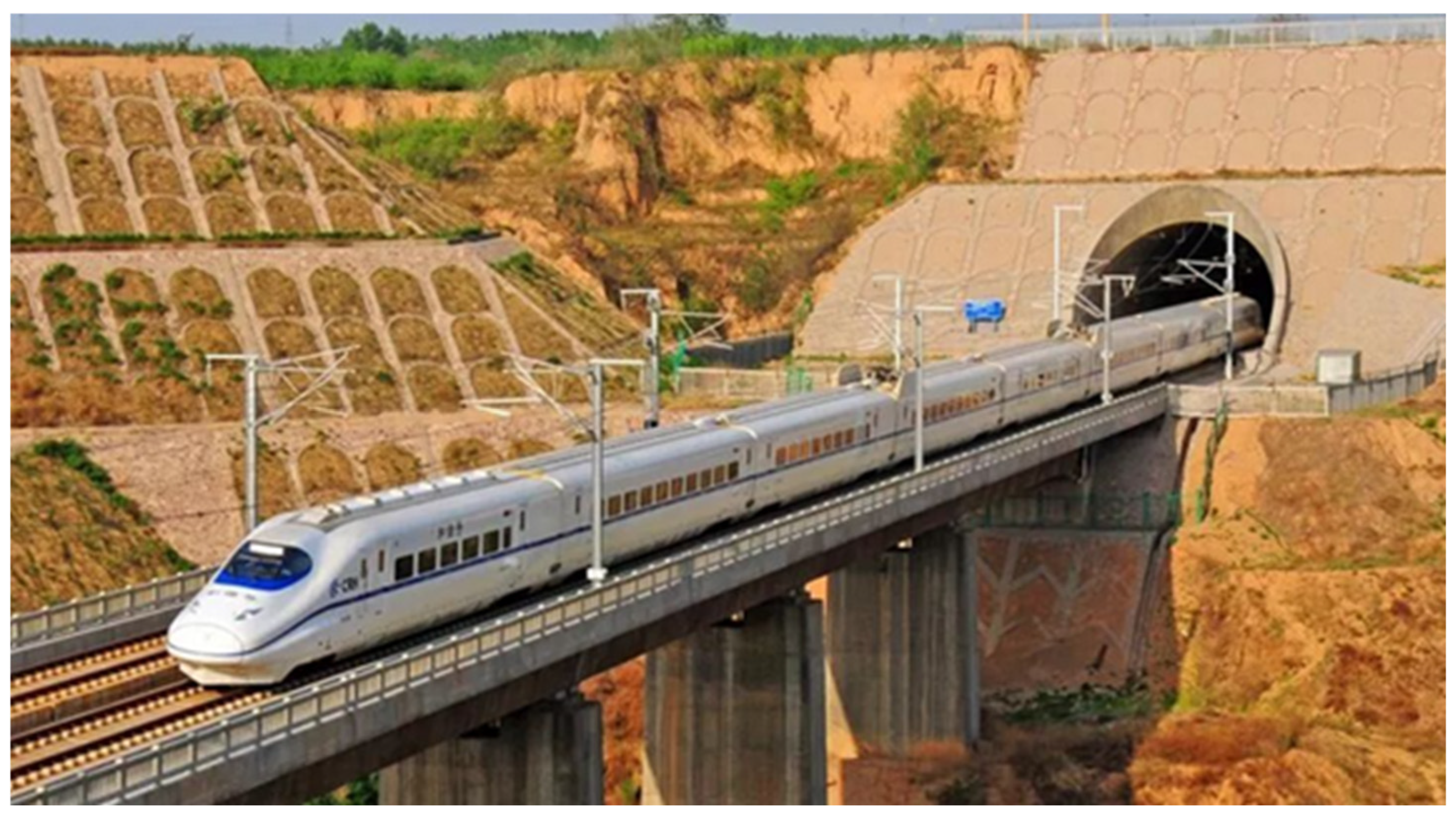
Due to the confined and elongated geometry of tunnels, as shown in Figure 1, the piston wind induced by high-speed train movement substantially modifies the internal flow field, thereby affecting the safety and effectiveness of tunnel ventilation systems. Therefore, investigating aerodynamic force fluctuations on the pantograph at 400 km/h is crucial. Using computational fluid dynamics (CFD), we calculated the aerodynamic lift of the pantograph at 350 km/h based on empirical formulas. A high-speed aerodynamic lift model for the pantograph was established using the empirical formula [6]. Aerodynamic forces significantly influence pantograph–catenary contact force [7]. Carnevale et al. examined differences in aerodynamic forces on the pantograph under open and closed operating conditions through numerical simulations [8]. Bocciolone et al. explored aerodynamic effects on pantograph–catenary interaction and optimized the pantograph head shape at 250 km/h to achieve a balance between drag and lift coefficients [9]. Pombo et al. employed a continuous contact force model with a penalty function to analyze pantograph aerodynamic characteristics under various wind attack angles [10]. Carnevale et al. applied the k–omega SST turbulence model, validated by wind tunnel data, to predict and evaluate pantograph aerodynamic performance, providing insights for aerodynamic design and optimization [11]. The renormalization group (RNG) k–ω turbulence model is used to investigate slipstream effects to ensure safe train operations under high-speed conditions [12]. Song et al. systematically investigated pantograph–catenary interaction dynamics across a range of speeds via experimental testing and numerical modeling. By integrating a neural network-based optimization algorithm, they improved contact force stability, achieving a 25% reduction in standard deviation at 380 km/h. This improvement significantly enhances the reliability of high-speed railway power supply systems [13].

Meanwhile, Tan. et al. employed Large Eddy Simulation (LES) and the Ffowcs Williams–Hawkings (FW–H) equation to analyze vortex structures and sound source energy distribution [14]. LES results show that vortex structures in the pantograph base frame and head region account for 92% of sound source energy, with low-frequency large vortices dominating noise radiation. Mandelli et al. compared Detached Eddy Simulation (DES) results with experimental data to analyze turbulent kinetic energy transport mechanisms, verifying the DES model’s applicability [15].

In summary, research on aerodynamic characteristics of pantographs at speeds around 400 km/h remains limited. Therefore, this paper quantitatively analyzes aerodynamic lift and drag generated by each pantograph component in the flow field. By comparing lift and drag values of individual components, the pantograph head is the most aerodynamically unstable part. Subsequently, overall turbulence simulations of the pantograph reveal turbulence behavior at the pantograph head, indicating that vortex shedding is the primary cause of lift variations at the head. These findings corroborate each other, confirming that the pantograph head is most susceptible to high-speed flow influences and suggesting a research direction for aerodynamic force fluctuations in pantographs for future trains operating around 450 km/h.

2. Pantograph Aerodynamic Simulation Model

This section describes the establishment of the flow-field model and the modeling approach for the pantograph aerodynamic model. Since the train operates at 400 km/h (Mach > 0.3), the fluid is treated as compressible. Consequently, a compressible-flow aerodynamic model is proposed.

Although compressibility has limited impact on overall aerodynamic performance, it cannot be neglected for detailed flow-field parameters such as surface pressure distribution [16]. Simulations under identical computational conditions were performed for both compressible and incompressible flow cases. Results show that at 400 km/h or above, aerodynamic lift from incompressible simulations is consistently lower than from compressible simulations. In current designs, the railway pantograph uses an articulated frame, essentially a four-bar linkage. For compressible flow, pantograph aerodynamic lift varies with air temperature; specifically, lift increases significantly as temperature decreases. In contrast, for incompressible flow, temperature variations have no effect on pantograph aerodynamic lift. Moreover, incompressible simulations inherently overlook air-density changes caused by compression around a moving blunt body at high speed. In real-world operations, flow-field density variations also alter aerodynamic lift. In China’s vast railway environments with significant temperature variations along routes, discrepancies between compressible and incompressible flow results become more pronounced, especially at 400 km/h. Therefore, under the high-speed conditions considered, compressible flow simulations are adopted to ensure accurate representation of aerodynamic lift behavior [17].

2.1. Pantograph Model

As train speed increases, pantograph–catenary interaction intensifies, and the catenary’s influence on the pantograph response grows significantly [18,19], posing potential risks to the pantograph’s structural safety during operation. To address this, Xu et al. proposed a neural network-based optimization method to minimize maximum stress and deformation of the pantograph under 400 km/h operating conditions, thereby satisfying structural strength requirements for high-speed operation [20]. Similarly, maintaining good contact is crucial for reducing failures in pantograph–catenary systems [21,22].

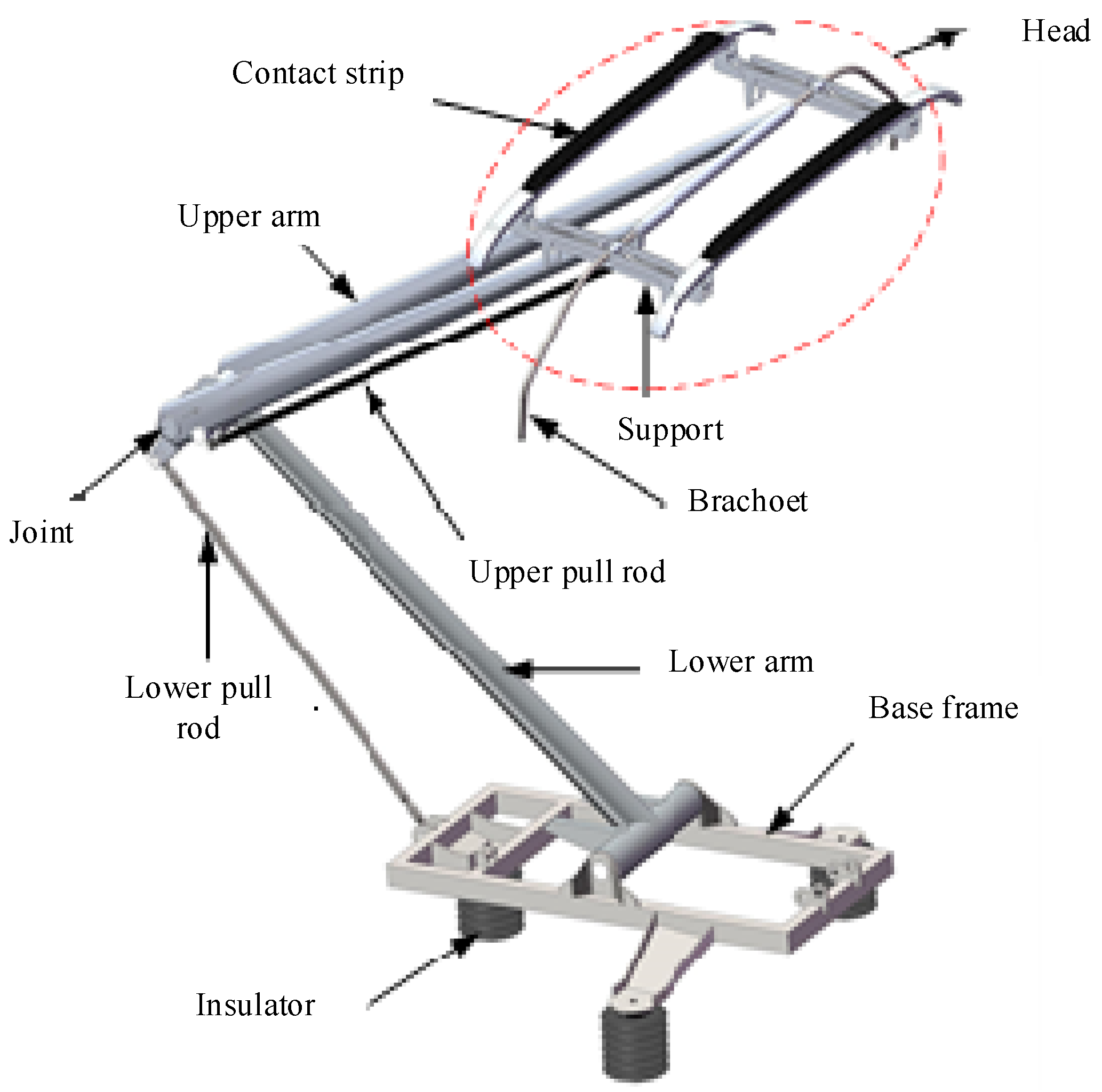
This study focuses on the DSA380 pantograph, widely used in China’s high-speed railways and manufactured by CRRC. This pantograph meets operational requirements at 400 km/h and has a height of 1680 mm. Its main components, shown in Figure 2, include the head, frame, base, and transmission system. The base attaches to the train roof and connects to the head via upper and lower arms; the head slider contacts the catenary, forming a frame structure that enables vertical movement.

Pantograph components interact via lift and drag forces generated by the wind field. The preload force between the pantograph head and the catenary ensures continuous sliding contact of the slider’s upper surface with the catenary. Damping and stiffness between the pantograph head and upper frame, and between upper and lower frames, control the pantograph’s vertical displacement. Under wind-field influence, lift variations must satisfy contact-force requirements to prevent excessive contact force or loss of contact. This study uses Fluent to embed the established pantograph model in a specified flow field and simulate surface turbulence distribution using the chosen CFD model. The time history of pantograph lift force is computed. Analysis reveals that aerodynamic lift fluctuations primarily arise from wind-induced vibrations due to turbulence shedding at the pantograph head and a high lift-to-drag ratio.

2.2. CFD Modeling of Pantograph

Generally, computational fluid dynamics (CFD) is widely used to study aerodynamic characteristics of high-speed train geometries. Traditional CFD methods start from the Navier–Stokes equations, which describe fluid flow behavior under the continuum assumption.

Compared to conventional aerodynamic simulations, CFD of high-speed train pantographs is more complex. The geometry of pantograph components creates intricate flow effects, with airflow interactions between parts. Moreover, boundary-layer separation on each component causes varying degrees of vortex shedding. In practice, the pantograph head is not streamlined; for example, its carbon slider has a rectangular cross-section. To ensure stable contact with the catenary, the slider is not designed with a streamlined cross-section. Furthermore, hinge joints between upper and lower frames have circular cross-sections, adding complexity to the wind-field environment around the pantograph.

Pantograph modeling is based on its actual structure, with the relationships between components playing a crucial role. Among pantograph components, larger frame structures contrast with smaller rod elements. Therefore, in CFD simulations, precise modeling and high-quality meshing are essential to capture the pantograph’s actual motion in the flow field. Considering the turbulent characteristics around pantograph components, all simulations use a pressure-based transient solver.

Since the train operates at the speed of 400 km/h, air is modeled as a compressible fluid. The CFD model employs a compressible flow field and is compared with incompressible models to demonstrate the advantages of compressibility at high speeds. The study assesses lift and drag on five main pantograph components, evaluating each component’s individual contribution to total aerodynamic forces. Analysis of lift-to-drag ratios reveals that the pantograph head is most significantly affected by aerodynamic force fluctuations. LES applies low-pass filtering to the Navier–Stokes equations to derive equations for large-scale turbulent motions, often used to simulate large vortices [23]. In contrast, DNS is more suitable for low-Reynolds-number flows, providing detailed turbulent flow information for engineering applications. However, simulating high-Reynolds-number flows with Direct Numerical Simulation (DNS) requires significant computational resources, limiting DNS applicability. RANS equations are derived by averaging the Navier–Stokes equations to describe mean turbulent quantities and are often solved with the Shear Stress Transport (SST) turbulence model. Compared to DNS, both RANS and LES require less computational effort.

2.3. Selection of CFD Models

For pantograph-specific turbulent flow modeling, DNS is primarily used. Available fluid simulation methods include Large Eddy Simulation (LES) and Reynolds-Averaged Navier–Stokes (RANS). Tian et al. established the relationship between Reynolds number and the mean velocity gradient, and compared the predictive performance of various turbulence models [24].

Since the airflow is treated as compressible, the Navier–Stokes equations remain valid within to the control volume surrounding the pantograph. For a compressible flow field, the turbulent kinetic energy and dissipation rate equations are derived from the averaged and instantaneous energy equations for compressible flow:

$${\displaystyle \frac{\partial \left(\rho k\right)}{\partial t}}+{\displaystyle \frac{\partial \left(\rho u_{i}k\right)}{\partial x_i}}={\displaystyle \frac{\partial }{\partial x_j}}\left[\left(\mu +{\sigma }_k{\mu }_t\right){\displaystyle \frac{\partial k}{\partial x_j}}\right]+P_k-{\beta }^{*}\rho k\omega$$

(1)

$${\displaystyle \frac{\partial \left(\rho \omega \right)}{\partial t}}+{\displaystyle \frac{\partial \left(\rho u_i\omega \right)}{\partial x_i}}={\displaystyle \frac{\partial }{\partial x_j}}\left[\left(\mu +{\sigma }_{\omega }{\mu }_t\right){\displaystyle \frac{\partial \omega }{\partial x_j}}\right]+P_{\omega }-D_{\omega }+Y_{\omega }$$

(2)

where

ρ represents the fluid density;

t represents the time;

ω represents the turbulent kinetic energy dissipation rate;

$k={\displaystyle \frac{1}{2}}\overline{{\mu }_i^{\prime }{\mu }_i^{\prime }}$ represents the turbulent kinetic energy per unit mass;

${\mu }_t=\rho C_{\mu }{\displaystyle \frac{k^2}{\epsilon }}$ represents the turbulent viscosity;

$P_k={\tau }_{ij}^t{\displaystyle \frac{\partial {\mu }_i}{\partial x_j}}$;

$P_{\epsilon }=C_1{\displaystyle \frac{\epsilon }{k}}{\tau }_{ij}^t{\displaystyle \frac{\partial {\mu }_i}{\partial x_j}}$;

$D_k=\rho \epsilon$;

$D_{\epsilon }=C_2\rho {\displaystyle \frac{{\epsilon }^2}{k}}{P}_{\epsilon }$ represents the turbulence production term;

$P_k$ represents the production term;

$D_{\epsilon }$ represents the turbulence dissipation term;

$D_k$ is the turbulence dissipation term.

Equations (1) and (2) represent two-equation models widely used in engineering practice. The empirical constants σ_k, σ_ε, C₁, C₂, and C_µ are 1.0, 1.3, 1.44, 1.92, and 0.09, respectively.

For high Reynolds number flows, the k–ε two-equation turbulence model is commonly employed. However, in the near-wall region adjacent to the pantograph surface, the local Reynolds number is low and viscous effects dominate. Therefore, the near-wall region requires treatment via methods such as wall functions.

In low-Reynolds-number near-wall regions, the k–ω turbulence model is used, while the standard k–ε model is applied in regions away from the pantograph surface. Therefore, the SST k–ω turbulence model is well-suited for flow scenarios involving a wide range of Reynolds numbers.

The transport equation for turbulent kinetic energy k in the SST k–ω turbulence model is

$${\displaystyle \frac{\partial k}{\partial t}}+{\mu }_t{\displaystyle \frac{\partial k}{\partial x_t}}={\displaystyle \frac{\partial }{\partial xt}}\left[\left(\mu +{\sigma }_k{\mu }_t\right){\displaystyle \frac{\partial k}{\partial x_j}}\right]+P_k-{\beta }^{*}k\omega$$

(3)

$${\displaystyle \frac{\partial \left(\rho \omega \right)}{\partial t}}+{\displaystyle \frac{\partial \left(\rho u_t\omega \right)}{\partial x_t}}={\displaystyle \frac{\partial }{\partial x_t}}\left[\left(\mu +{\displaystyle \frac{{\mu }_t}{{\sigma }_{\omega }}}\right){\displaystyle \frac{\partial \omega }{\partial x_t}}\right]+P_{\omega }-D_{\omega }+Y_{\omega }$$

(4)

where P_ω denotes the turbulence production term; D_ω denotes the turbulence dissipation term; and Y_ω denotes the turbulence cross-diffusion term.

Because the pantograph structure mainly comprises bluff-body components, it inherently generates large-scale flow separation and unsteady vortex shedding in the surrounding flow field. A common numerical approach for these cases is Detached Eddy Simulation (DES). This hybrid approach uses a Reynolds-Averaged Navier–Stokes (RANS) model for near-wall regions where turbulence scales are smaller than local grid dimensions. When turbulence length scales exceed grid resolution, the Large Eddy Simulation (LES) formulation is activated to capture dominant unsteady vortical structures. The LES region typically encompasses the turbulent core dominated by large-scale coherent structures, while RANS remains in near-wall boundary layers. This dual-resolution strategy significantly relaxes the stringent grid requirements of pure LES. DES combines the wall-modeling capabilities of the SST k–ω turbulence model with capability of LES to capture unsteady, large-scale turbulence. Pressure–velocity coupling uses the SIMPLE (Semi-Implicit Method for Pressure-Linked Equations) algorithm, ensuring numerical stability for unsteady flows.

The RANS model is well suited to assess interactions among pantograph components and their aerodynamic lift performance in a compressible flow field. Steady-state simulation is well suited for this scenario. Moreover, steady-state simulations based on RANS simulations demonstrate good performance in aerodynamic analyses at different pantograph working heights [25].

2.4. Computational Domain and Boundary Conditions

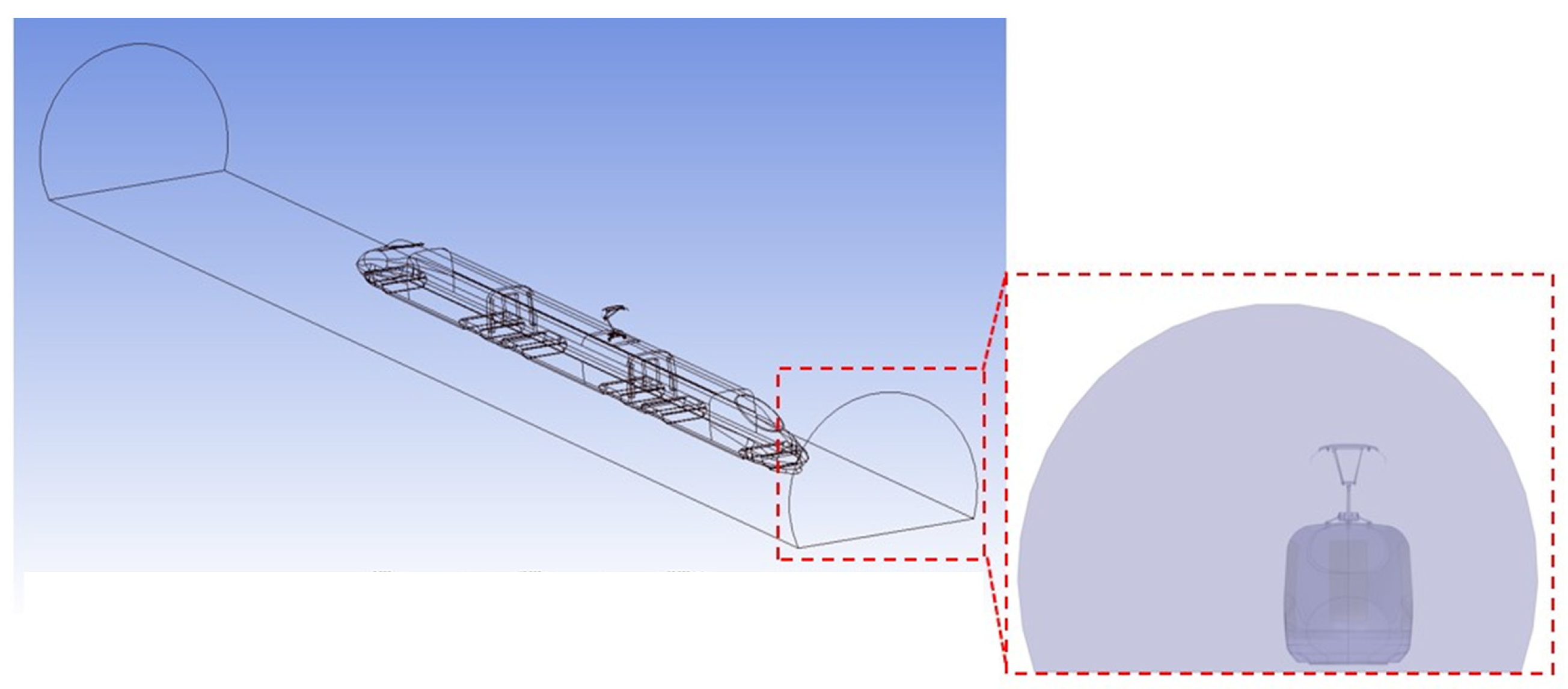
Studies [26] employed various methods to reconstruct spatially distributed wind fields from empirical wind speed spectra. These wind fields were then utilized to compute the unsteady aerodynamic loads on the pantograph during high-speed operation. Figure 3 shows the computational domain used to simulate the wind tunnel test at 400 km/h. The upstream boundary is defined as a velocity inlet, while the downstream boundary is treated as a pressure outlet. To minimize computational effort, the left, right, and top boundaries are designated as symmetry planes, representing the interface with the atmosphere and avoiding the need to resolve wall boundary layers. The ground is modeled as a rigid wall. The pantograph is mounted on the train roof, which has an arc-shaped cross-section. The specific boundary conditions for this computational domain are detailed in

Table 1. Boundary condition adopted for the CFD simulation (pressure p and velocity U).

Boundary Conditions Patch Name	p	U
Inlet	$\nabla p=0$	$U_0$
Outlet	0	$\nabla U=0$
Roof	$\nabla p=0$	0
Wall	$\nabla p=0$	0
Sym	Symmetry plane	0
Pantograph surface	$\nabla p=0$	0

.

The computational domain is designed to simulate the aerodynamic performance of the pantograph at 400 km/h, including the pantograph and its surrounding flow field. The front face is set as a velocity inlet at 400 km/h, with zero pressure gradient normal to the boundary, allowing pressure to adjust to the flow field. The rear face is designated as a pressure outlet with specified average pressure and zero velocity gradient normal to the boundary, ensuring free fluid exit. The left, right, and top boundaries are set as symmetry planes (zero flow), reducing computational cost. The bottom, representing the ground, is modeled as a no-slip wall with near-zero velocity and pressure determined by the flow field. The pantograph surface is modeled as a no-slip wall with zero velocity and pressure determined by the flow field.

This boundary condition configuration effectively captures key flow-field characteristics around the pantograph while simplifying computation via symmetry planes. Using a compressible flow solver to account for density variations ensures simulation accuracy. Additionally, mesh refinement around the pantograph improves boundary-layer and wake resolution, balancing accuracy and computational accuracy and efficiency.

2.5. Mesh Sensitivity

Considering the pantograph’s complex structural geometry, tetrahedral meshes are used outside the boundary layer to reduce meshing computational cost. Polyhedral meshes are employed in the outer region to leverage their flexibility. Data exchange between internal and external flow domains is facilitated via polyhedral and hexahedral meshes.

In the overall computational domain, a single-stage Body of Influence (BOI) refinement is applied once around the pantograph. The base mesh size is H, and the refined region mesh size is H/8. Considering the pantograph’s surface complexity, the surface mesh size is set to 0.5 mm to balance computational accuracy and efficiency. To achieve a target y+ close to 1, the first boundary-layer height is set to 3.4877 × 10⁻⁶ m, with 27 boundary layers, yielding a total boundary-layer thickness of 2.2602 × 10⁻³ m. Compressible flow parameters from numerical simulations are presented in

Table 2. Compressible flow parameters.

Parameter	Value
Molecular weight/(kg·kmol−1)	28.966 × 103
Specific heat capacity/(J·kg−1 K−1)	100.58
Thermal conductivity/(W·m−1 K−1)	0.0242
Viscosity coefficient/(kg·m−1 s)	1.7889 × 10−5
Temperature/K	305.15

.

Due to computational constraints, indefinitely refining the mesh to its smallest divisions is not feasible. Therefore, selecting an appropriate mesh size to ensure adequate simulation accuracy is necessary. This study investigated the impact of mesh resolution on results by employing three refinement strategies. Flow fields were computed for varying mesh densities, balancing accuracy and computational cost. Considering the need to balance accuracy and computational cost—and given our laboratory’s dual-socket AMD 7763 system with 512 GB RAM—we selected a mesh cell size of 100 mm. The mesh comprised 42.762 million elements with a growth rate of 1.2. Figure 4 illustrates the pantograph’s placement within the flow-field mesh. This configuration required 324 GB of memory during computation, demonstrating efficient use of available resources.

3. CFD Simulation Results

The pressure distribution on the pantograph surface at the train speed of 400 km/h is illustrated in Figure 5. Figure 6 shows that in compressible-flow simulations, a pronounced pressure difference occurs at the front slider and arm of the pantograph. This phenomenon arises from boundary-layer separation: the fluid boundary layer detaches from the pantograph surface and, due to velocity discrepancies with the surrounding free-stream flow, generates wake turbulence. Under an adverse pressure gradient, boundary-layer kinetic energy decreases, ultimately causing separation. As shown in the pressure distribution diagram, using an appropriate number of boundary-layer mesh layers in compressible-flow simulations yields a more accurate and detailed representation of pantograph surface pressure.

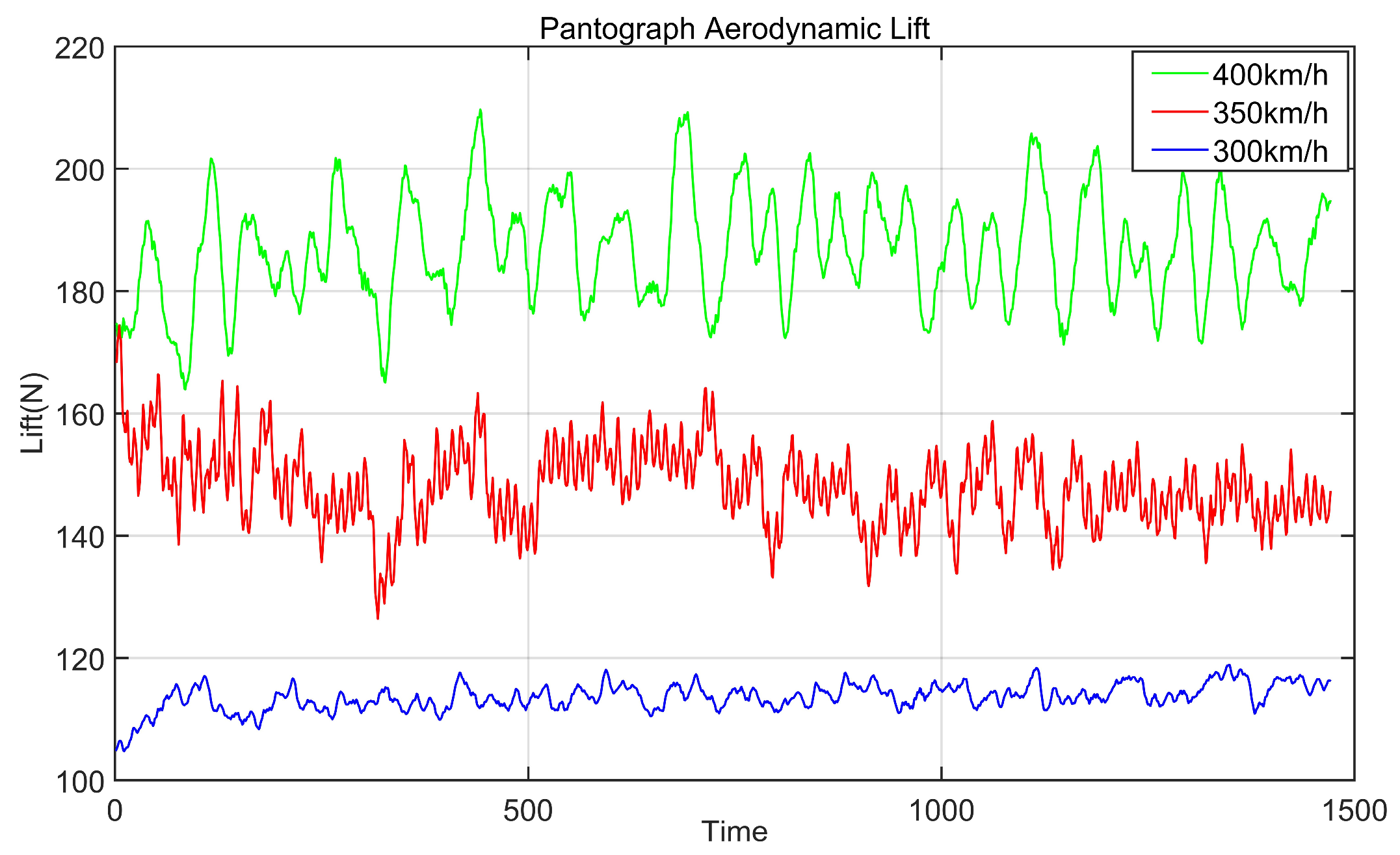
Simulations at inlet velocities of 300, 350, and 400 km/h were conducted to investigate pantograph aerodynamic lift variations at different speeds, shown in Figure 7. Simulation results at different speeds agree with data from reference [27], verifying their accuracy. The Fast Fourier Transform (FFT) of pantograph lift at 300, 350, and 400 km/h (Figure 8) reveals significant spectral peaks, indicating dominant frequency components in the lift signal. The analysis results indicate the following:

• At 300 km/h, the aerodynamic lift force fluctuation of the pantograph ranges between 108 and 119 N. The primary peak occurs at approximately 1–2 Hz with an amplitude of about 1–2 N, weaker secondary peaks appear between 5 and 10 Hz with amplitudes below 1 N. Above 10 Hz, amplitudes drop rapidly to near zero, indicating negligible high-frequency components. This suggests a narrow frequency range of lift fluctuations at 300 km/h. Additionally, smooth behavior at this speed indicates greater system stability at lower speeds.
• At 350 km/h, the aerodynamic lift force fluctuation of the pantograph ranges between 126 and 166 N. The primary peak appears around 1–2 Hz with an amplitude of approximately 2–3 N; multiple secondary peaks occur between 5 and 15 Hz with amplitudes of 0.5–1.5 N. These secondary peaks in the 5–15 Hz range are primarily linked to pantograph–catenary dynamic interaction.
• At 400 km/h, the aerodynamic lift force fluctuation of the pantograph ranges between 164 and 210 N. The primary peak remains at about 1–2 Hz, but its amplitude increases to 4–5 N; secondary peaks are present but with lower amplitudes. Above 10 Hz, amplitudes decrease sharply to near zero, indicating minimal contribution of high-frequency components at 400 km/h.

Figure 7. Aerodynamic lift fluctuations of the pantograph at speeds of 300 km/h, 350 km/h, and 400 km/h.

Figure 7. Aerodynamic lift fluctuations of the pantograph at speeds of 300 km/h, 350 km/h, and 400 km/h.

Figure 8. Spectral analysis of pantograph aerodynamic lift at speeds of 300 km/h, 350 km/h, and 400 km/h.

Figure 8. Spectral analysis of pantograph aerodynamic lift at speeds of 300 km/h, 350 km/h, and 400 km/h.

The peak lift fluctuation amplitude is highest at 400 km/h (approximately 5 N), followed by 350 km/h (approximately 3 N), and lowest at 300 km/h (approximately 2 N). Peak amplitude increases with speed, reflecting intensified aerodynamic lift fluctuations at high speeds. This demonstrates that as speed increases, airflow disturbances intensify, potentially heightening pantograph–catenary contact instability. In particular, the notably high amplitude at 400 km/h suggests the need for enhanced aerodynamic lift control at ultra-high speeds to prevent pantograph–catenary separation and associated safety hazards. To meet growing operational safety requirements of high-speed railway systems—especially at speeds approaching or exceeding 400 km/h—fundamental research must be intensified to elucidate pantograph–catenary aerodynamics. Under wind load, contact wire galloping caused by aerodynamic instability may produce large amplitudes, posing a significant threat to normal railway operation [2].

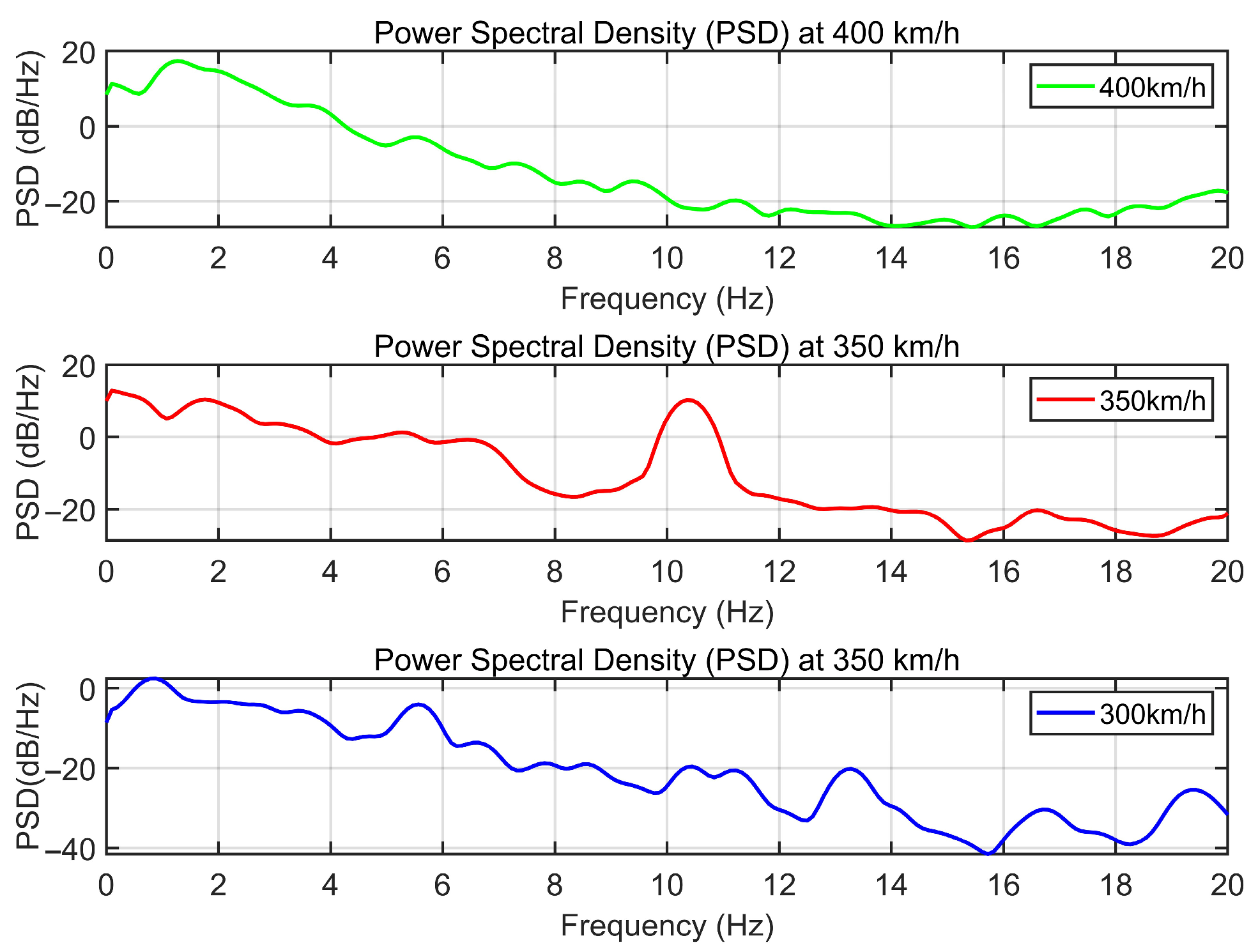
Figure 9 illustrates that at 400 km/h, the power spectral density (PSD) reaches its maximum peak at approximately 1.5–2 Hz, with a value of around 10 dB/Hz. Above 10 Hz, the PSD decreases rapidly to below 20 dB/Hz, approaching the noise floor. This indicates that the energy of lift fluctuations during high-speed operation is primarily concentrated in the low-frequency range. A similar trend is observed at lower speeds: the PSD peak is highest at 400 km/h (approximately 10 dB/Hz), followed by 350 km/h (around 5 dB/Hz), and lowest at 300 km/h (near 0 dB/Hz). The increase in spectral power with speed reflects that the energy associated with aerodynamic lift fluctuations grows with train velocity. These aerodynamic disturbances serve as a major contributor to instability in the pantograph–catenary contact force under high-speed operating conditions.

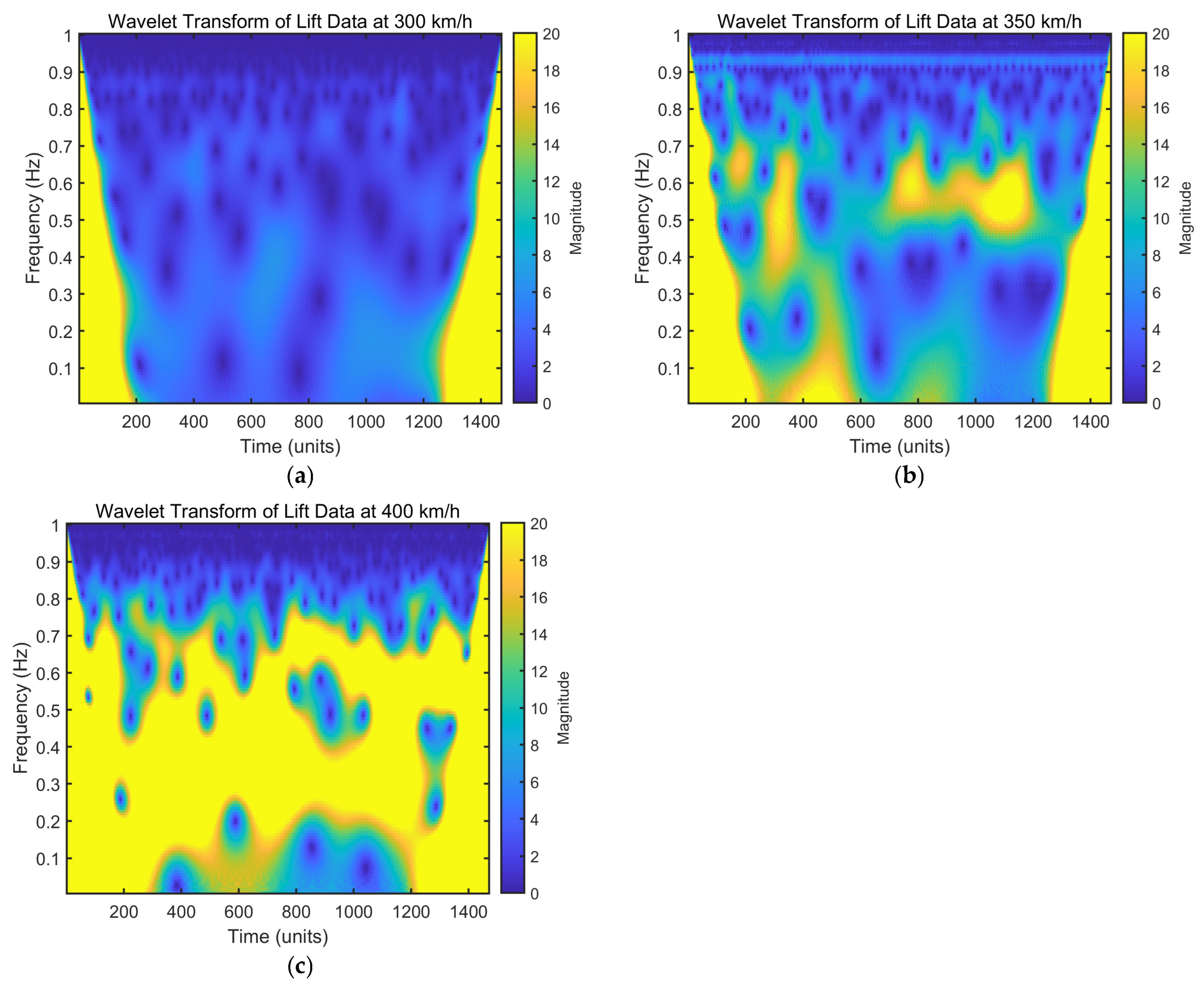
Figure 10 illustrates the time–frequency characteristics of the aerodynamic lift acting on the pantograph at train speeds of 300 km/h, 350 km/h, and 400 km/h, respectively. It can be seen from Figure 9 that at 300 km/h, the dominant frequency components of the aerodynamic lift are concentrated between 0.1 Hz and 0.3 Hz, with relatively low amplitudes (primarily in the blue range, 0–4). The frequency distribution remains uniform across the time domain, with no prominent periodic high-amplitude regions. This indicates stable aerodynamic lift behavior and minimal flow disturbances. Frequencies above 0.5 Hz exhibit negligible amplitudes, suggesting the absence of significant high-frequency vibrations.

At 350 km/h, the dominant frequencies remain between 0.1 Hz and 0.3 Hz, but there is a noticeable emergence of mid-frequency components (0.3 Hz to 0.5 Hz) with increased amplitudes (partially in the green range, reaching 6–8). While the time–frequency distribution is still relatively uniform, localized amplitude enhancements begin to appear. This implies increasing complexity in lift fluctuations, likely associated with flow separation or vortex formation. Additionally, sparse amplitudes appear in the high-frequency range (>0.5 Hz), marking the onset of high-frequency vibrations as speed increases.

At 400 km/h, the dominant lift frequencies remain within 0.1 Hz to 0.3 Hz, but both mid-frequency (0.3 Hz to 0.5 Hz) and high-frequency (0.5 Hz to 1 Hz) components intensify significantly. Amplitudes increase markedly, with yellow regions (amplitudes of 10–20) emerging in the 0.3–0.5 Hz band. Periodic high-amplitude regions are clearly visible along the time axis, indicating stronger periodic behavior in lift fluctuations. This can be attributed to enhanced turbulence or intensified pantograph–catenary interaction. In the high-frequency band, amplitudes rise substantially (green to yellow, 8–20), reflecting significant high-frequency vibrations induced by increased flow instability.

4. Numerical Simulation of Turbulence for Pantographs

However, lift fluctuations are influenced not only by the average lift force but also by turbulence effects, which are strongly dependent on the square of the flow velocity. As the train speed increases, the turbulence intensity in the surrounding flow field significantly intensifies, particularly around the pantograph head. Due to its non-streamlined design, phenomena such as boundary-layer separation and vortex shedding become more prominent, leading to further amplification of the dynamic lift fluctuation amplitude.

Turbulence is an inevitable phenomenon in the operation of high-speed train pantographs, especially at speeds of 400 km/h. It primarily arises from the complex geometric features of the pantograph (such as the rectangular cross-section of the slider and the cylindrical arms), as well as from interactions with the wake flow generated by the train head. According to the study employing the SST turbulence model in reference [11], both the turbulent kinetic energy (k) and turbulence dissipation rate (ω) around the pantograph increase significantly with speed. At 300 km/h, turbulence is mainly characterized by low-frequency fluctuations induced by localized boundary-layer separation. In contrast, at 400 km/h, the turbulence intensity rises markedly, and higher-frequency vortex shedding becomes the dominant contributor to lift fluctuations.

4.1. Numerical Simulation of Pantograph Components

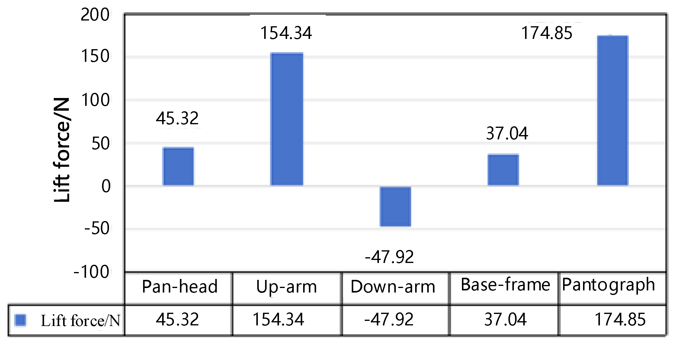
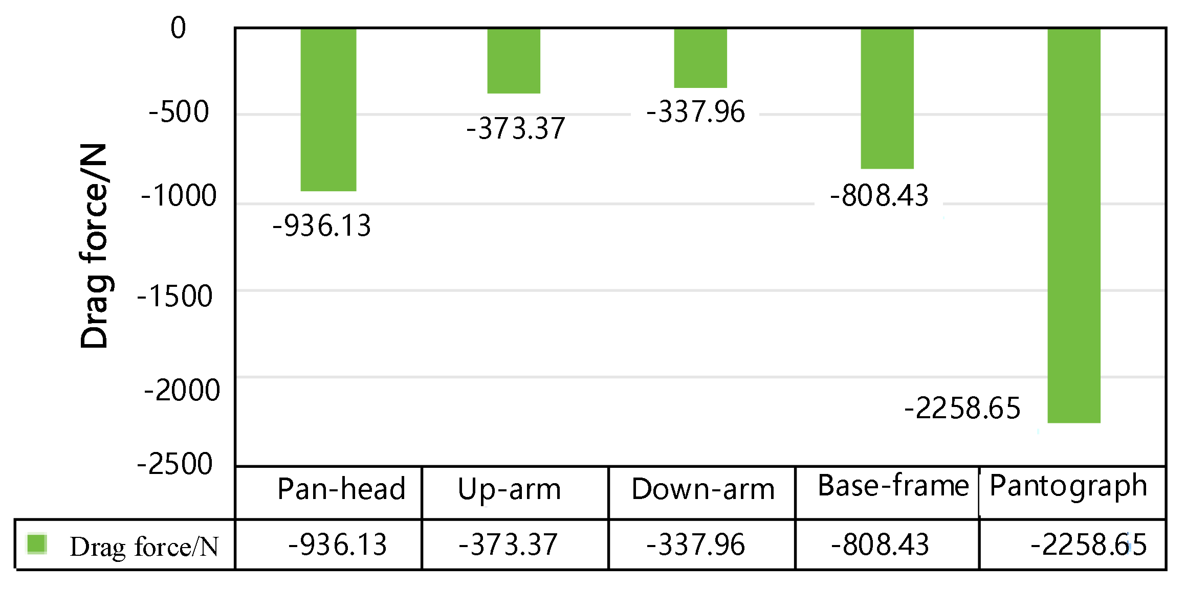
To analyze the influence of different pantograph components on the overall aerodynamic performance, separate simulations were conducted for each major part, specifically, the pantograph head, upper arm, and lower arm. The simulation results are shown in Figure 11, and the corresponding aerodynamic lift and drag values are presented in

Table 3. Lift, drag, and lift-to-drag ratios of pantograph components at 400 km/h.

Component	Lift Force/N	Drag Force/N	Lift-to-Drag Ratio
Pan-head	45.32	−936.13	0.0484
Up-arm	154.34	−373.37	0.4134
Down-arm	−47.92	−337.96	0.1418
Base	37.04	−808.43	0.0334
Pantograph	174.85	−2258.65	0.0774

.

Lee et al. investigated the aerodynamic force distribution of pantographs through wind tunnel testing, and measured the lift and drag forces of individual components [28]. Their findings demonstrate that the variation in lift-to-drag ratios among the components indicates differences in aerodynamic performance under identical flow conditions. In the aerospace domain, a higher lift-to-drag ratio is generally desirable, as it enables more efficient conversion of propulsive power into lift. However, in the context of pantograph–catenary interaction, greater lift is not inherently beneficial.

When individual pantograph components exhibit a low lift-to-drag ratio, it may undermine the stability of current collection performance. In particular, aerodynamic instability can arise at the pantograph head due to a combination of fluctuating vertical lift and substantial drag in the longitudinal (train movement) direction. This instability can induce variations in the contact force between the pantograph and catenary, leading to performance degradation or contact loss. Therefore, identifying and analyzing these instability-inducing aerodynamic conditions is essential. Simulation results confirm that the pantograph head has the lowest lift-to-drag ratio among all components, confirming that this region is particularly vulnerable to aerodynamic force fluctuations caused by flow-field disturbances.

4.2. Validation of Aerodynamic Lift and Drag Simulation

The sum of the aerodynamic lift calculated from individual pantograph components (188.78 N) accounts for 90.2% of the total lift obtained from the full pantograph simulation (174.85 N); both lift values remain within the fluctuation range of 164 to 210 N shown in Figure 7. For drag, the total from the individual components reaches 111.67% of the full-system drag. These results validate the reliability of the lift and drag estimations for each component.

As illustrated in Figure 12 and Figure 13, the pantograph head exhibits the lowest lift-to-drag ratio among all components. This implies an excessively large proportion of aerodynamic drag relative to lift, indicating that the aerodynamic forces acting on the head are inherently unstable. Moreover, since the head is positioned at the terminal end of the pantograph linkage system and is the direct point of contact with the catenary, it is especially vulnerable to aerodynamic disturbances.

4.3. Turbulence Induced by the Pantograph

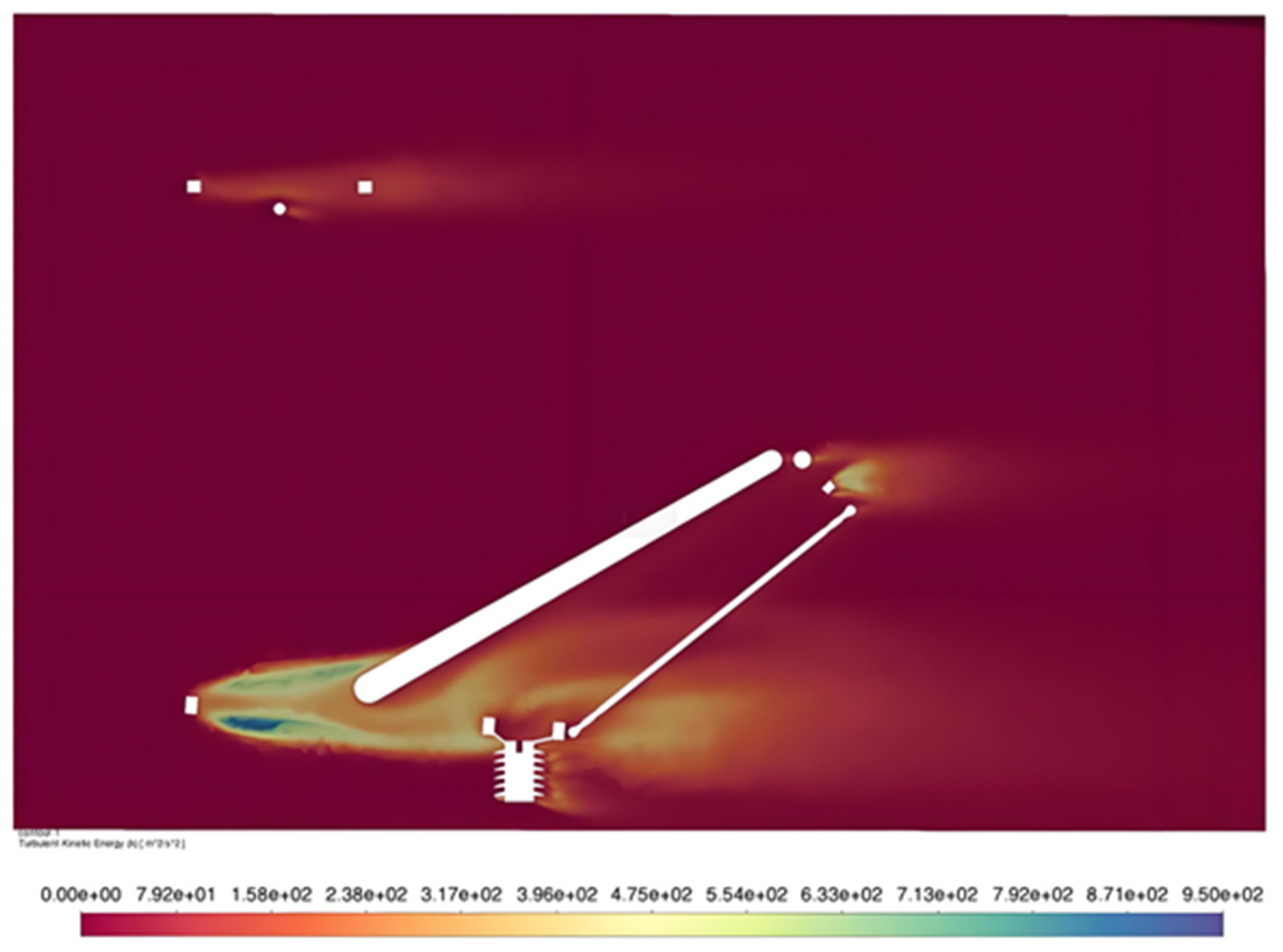
As a bluff-body configuration composed of interconnected rods, the pantograph induces complex flow phenomena when exposed to high-speed airflow. The flow decelerates around its structure, leading to both wall friction and pressure drag caused by changes in flow velocity. These aerodynamic resistances collectively impede the fluid motion. When the boundary layer on the pantograph surface is reduced to nearly zero by these effects, the wall shear stress drops accordingly. However, the external pressure gradient remains, driving the fluid to reverse direction. This results in flow separation and backflow, wherein the reversed flow detaches from the surface and interacts with the incoming stream. Since the incoming flow dominates in volume, it forces the backflow away from the surface, causing the boundary layer to grow thicker and ultimately separate. At high speeds, this boundary-layer separation becomes more intense and is a major contributor to turbulence, thereby destabilizing the aerodynamic behavior of the pantograph. A three-dimensional Gaussian Frandsen wake model incorporating wake effects and boundary-layer compensation allows accurate predictions of wind speed distribution in similar turbulent flow environments.

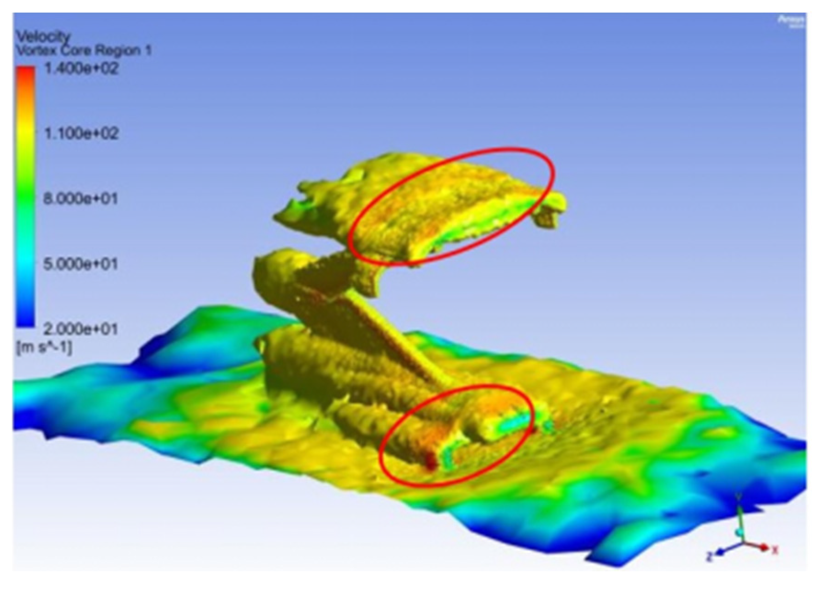
As illustrated in Figure 14, at 400 km/h, turbulence is primarily generated at the pantograph base frame, at the junctions of the upper and lower arms, and around the pantograph head. Among these, the base frame and pantograph head are identified as the dominant turbulence sources, as indicated by the red circle in Figure 14. However, because the base frame is rigidly mounted to the vehicle roof, its wind-induced vibrations are largely absorbed by the train body, which possesses a significantly higher mass [29]. In contrast, the pantograph head, as the terminal part of the linkage system, cannot rely on the vehicle body to dissipate vibrational energy. 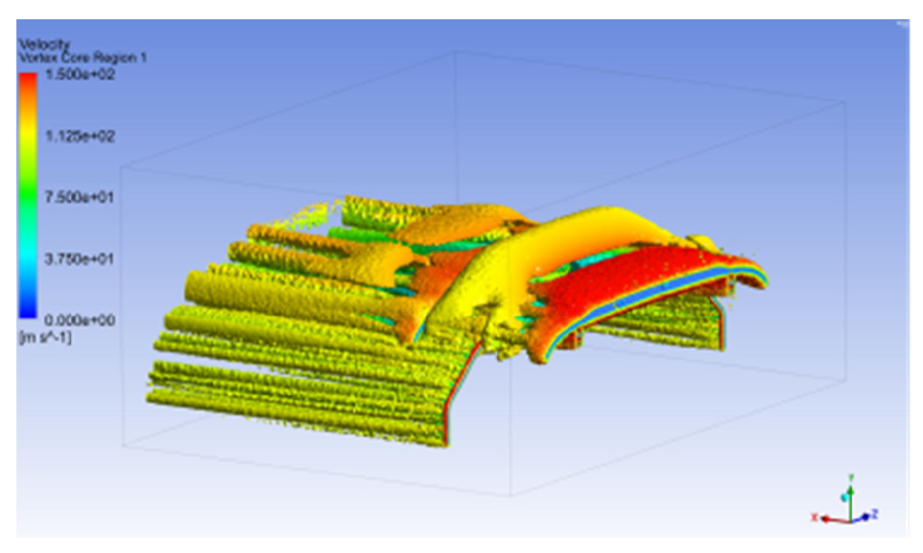This makes it the most critical site for wind-induced vibration in the pantograph system, as confirmed in Figure 15.

The instability of flow separation and vortex shedding near the pantograph head directly drives fluctuations in aerodynamic forces. As measurement points in the velocity profile approach the head’s edge, the energy associated with vortex shedding significantly increases. These unsteady flow characteristics not only cause instability in lift force but also generate high-frequency excitations that impair current collection performance.

In summary, the significant turbulence and unsteady flow observed at the pantograph head highlight that unstable boundary-layer separation and vortex shedding are the dominant causes of aerodynamic force fluctuations. This corroborates earlier conclusions that the pantograph head, characterized by the lowest lift-to-drag ratio, is particularly susceptible to aerodynamic disturbances.

5. Conclusions

This study employs CFD to simulate the total aerodynamic lift and drag acting on a pantograph and compares results from individual component simulations with those of the complete pantograph assembly. Key findings include the following:

• Aerodynamic lift oscillations intensify markedly with increasing train speed. At 400 km/h, fluctuation amplitudes reach nearly 50 N, with dominant spectral energy concentrated in the low-frequency band. This underscores the importance of accounting for lift-force variability in future high-speed pantograph–catenary interaction analyses.
• Lift-to-drag ratios computed for each pantograph element reveal that the pantograph head has the lowest ratio, signifying the greatest susceptibility to aerodynamic force fluctuations. Localized flow separations around the head drive these pronounced oscillations.
• CFD analysis identifies the pantograph base frame and head as the primary turbulence-concentration regions at 400 km/h. Because the base frame is rigidly mounted to the vehicle body, its wind-induced vibrations are constrained and absorbed by the vehicle mass. Consequently, the pantograph head emerges as the dominant source of lift fluctuations.

This study advances understanding of pantograph performance under high-speed conditions. For designing and optimizing high-speed trains—especially those at 400 km/h or above—the effects of high-speed aerodynamic environments on the pantograph must be thoroughly considered. These considerations are critical for maintaining stable pantograph–catenary interaction, ensuring reliable power supply and safe current collection, and thus provide a theoretical basis for safe, rapid high-speed railway development.