Graphical Empirical Mode Decomposition–Convolutional Neural Network-Based Expert System for Early Corrosion Detection in Truss-Type Bridges

Abstract

Corrosion is a critical issue in civil structures, significantly affecting their durability and functionality. Detecting corrosion at an early stage is essential to prevent structural failures and ensure safety. This study proposes an expert system based on a novel methodology for corrosion detection using vibration signal analysis. The approach employs graphical empirical mode decomposition (GEMD) to decompose vibration signals into their intrinsic mode functions, extracting relevant structural features. These features are then transformed into grayscale images and classified using a Convolutional Neural Network (CNN) to automatically differentiate between a healthy structure and one affected by corrosion. To enhance the computational efficiency of the method without compromising accuracy, different CNN architectures and image sizes are tested to propose a low-complexity model. The proposed approach is validated using a 3D nine-bay truss-type bridge model encountered in the Vibrations Laboratory at the Autonomous University of Querétaro, Mexico. The evaluation considers three different corrosion levels: (1) incipient, (2) moderate, and (3) severe, along with a healthy condition. The combination of GEMD and CNN provides a highly accurate corrosion detection framework that achieves 100% classification accuracy while remaining effective regardless of the damage location and severity, making it a reliable tool for early-stage corrosion assessment that enables timely maintenance and enhances structural health monitoring to improve the long life and safety of civil structures.

1. Introduction

Most of the worldwide current operating highway bridges were built with steel or steel-reinforced concrete, and a significant percentage of them have surpassed or are close to exceeding their design service life [1]. In this sense, corrosion is one of the most common and dangerous damage types in steel bridges, which can lead to degradation of critical elements and the collapse of the whole structure [2]. Therefore, an efficient monitoring of bridges is fundamental for ensuring reliability, thus safeguarding the investments made in this kind of infrastructure and the lives of users.

Numerous accidents involving bridge collapses have occurred around the world with tragic consequences due to the existence of different types of damage that were not detected early enough [3]. Just to mention some of the most recent and tragic incidents where corrosion was the main factor that caused the downfall of bridges, the following two cases are mentioned: The Nanfang’ao Bridge suddenly fell down on 1 October 2019 in Yilan County, Taiwan; 6 people died, and 12 were injured. The corresponding investigations determined that the reason for the catastrophic failure was the presence of corrosion in critical elements combined with inadequate maintenance. At the moment of the collapse, the effective cross-sectional area of the supporting steel cables was estimated to be only 22% to 27% [4,5]. On the other hand, previously, on 14 August 2018, a long section of the Morandi Bridge, about 243 m, collapsed in Genoa, Italy, killing 43 people and injuring 16. Similarly to the previous case, this incident was primarily due to corrosion of the steel cables, which was increasing until the functional cross-sectional area of them was severely reduced; consequently, the entire structure was weakened, and, finally, the corresponding section failed, falling into a river [4,6]. Therefore, considering the terrible consequences of bridges’ collapses in terms of devastating human tragedies and substantial economic disruptions (mainly affecting infrastructure, trade, and employment), damage diagnosis and prognosis in bridges have been one the most studied topics in the research line of integrity assessment of infrastructures, whose main objectives are related to detection, localization, and severity evaluation of damage, as well as with the prediction of remaining service life and the decision making regarding maintenance plans for the analyzed structure [7]. Thus, the implementation of efficient, low-cost, automatic, and online methods to evaluate the structural condition of entire bridges, as part of a structural health monitoring (SHM) system, plays a fundamental role in avoiding fatalities on bridges [8].

Structural damage detection methods based on non-destructive testing (NDT) are local methods that offer valuable advantages, e.g., the integrity of the examined element is preserved since the evaluation can be performed without causing a damage, defects in early stages can be detected, material degradation can be monitored, the safety/reliability of the entire structure increases, cost-effectiveness is attractive, the environment is protected, etc [9]. Some of the most often used NDT techniques in the structures’ components are eddy current [10], magnetic particle [11], liquid penetrant [12], X-ray [13], ultrasound [14], and acoustic emissions [15], among others. However, they present several important challenges, including, for example: (i) the NDT inspections are not suitable to detect damage found inside the structural elements; (ii) they need direct access to the component to be evaluated and many of the critical elements of bridges are placed in locations with complicated accessibility; (iii) the examination quality depends significantly on the knowledge/experience of the inspector; (iv) the assessments are periodic and they do not provide information of the structural condition in real-time; and (v) they cannot determine a global integrity state of large civil structures. On the other hand, the global methods overcome the restrictions of the local methods, allowing the evaluation of entire civil structures. In this context, SHM systems involving global methods based on vibration signal processing to identify damage in bridges have been widely studied in recent decades due to their promising results [16], and they can be classified in a general manner as parametric and non-parametric methods [17].

Regarding parametric methods, various algorithms are employed to obtain the modal parameters and their derivatives from analyzed structures, which relate directly to the fundamental characteristics of structural dynamic behavior. Variations in these modal parameters, compared to the known baseline (healthy condition) of the studied bridge, can indicate the presence of structural damage [17]. The advantages of these methods are related mainly to their ability to provide quantitative damage assessment, sensitivity to local damage, potential for automation, and ease of updating models with new data [17]. Examples of parametric methods applied in civil infrastructure include techniques based on changes in natural frequencies, mode shapes, and modal damping [18], modal curvatures [19], modal strain energy [20], modal scale factors [21], modal assurance criterion [22], coordinate modal assurance criterion [23], enhanced coordinate modal assurance criterion [24], and stiffness separation method [25], among others. Despite the promising results achieved by parametric methods, they exhibit significant limitations. Notably, these include susceptibility to environmental conditions, the necessity for detailed mathematical or numerical structural models, and high computational time requirements [17].

On the other hand, non-parametric methods analyze vibrational responses measured directly from structures. By employing modern signal processing techniques, these methods can extract or enhance features associated with structural damage that might otherwise remain undetected [17]. Thus, non-parametric methods overcome several limitations inherent in parametric approaches, offering substantial advantages for practical application in real-world structures to identify damage efficiently, highlighting that they are suitable for working with non-stationary signals such as the signals obtained from civil structures, they require less prior knowledge about the structure, they are more robust to variations in operating and environmental conditions, and there is no need of complex structural models; however, their limitations are associated with the need of developing specific algorithms for each particular structure, selection of useful features, and the need of detailed analyses performed by a specialist, among others [17]. Examples of non-parametric methods applied to civil infrastructure include empirical mode decomposition (EMD) [26], multiple signal classification [27], fractal dimension analysis [28], time series modeling [29], wavelet transform analysis [30], principal component analysis [31], the Shannon entropy index [32], and the homogeneity index [33], among others. Additionally, various machine learning (ML) classifiers have been integrated into structural damage detection systems employing parametric and non-parametric global vibration methods, significantly enhancing the reliability and accuracy of infrastructure integrity assessments [34]. Prominent classifiers within this domain include artificial neural networks [35], support vector machines [36], and self-organizing maps [37], among others. However, despite their promising results, these ML-based methods still face notable challenges, including sensitivity to environmental conditions, the necessity for precise calibration, and dependence on expert knowledge for effective feature extraction and optimal classifier selection [38].

Recent advances in artificial intelligence, particularly in deep learning (DL), have opened new possibilities for overcoming limitations associated with conventional structural damage detection methods [39]. Convolutional Neural Networks (CNNs), a leading type of DL algorithm, have proven highly effective in analyzing and processing visual data, including images and videos [39]. CNNs automatically extract essential features and patterns from data through successive convolutional and pooling layers, making them especially suitable for SHM applications relying on visual signal representations [38]. For reliable performance, CNNs require input images that encapsulate meaningful and discriminative features relevant to the phenomenon being analyzed. In general, across various fields of study, this means the input data should effectively reflect the intrinsic dynamics of the underlying process, particularly when such processes exhibit nonlinear and non-stationary behavior. Ideally, this can be achieved without relying on extensive signal preprocessing or intensive calibration procedures. This requirement naturally leads to the use of EMD, a technique well-suited to extract such complex behaviors from raw signals. EMD, a prominent time–frequency signal processing technique proposed by Huang et al. [40], has emerged as a valuable tool for structural damage detection. EMD decomposes non-stationary (NS) and nonlinear (NL) vibration signals into intrinsic mode functions (IMFs), making it particularly relevant for analyzing structural responses, as measured signals from infrastructure that typically exhibit NS and NL characteristics. Traditionally, the IMFs extracted by EMD require careful expert analysis to determine their relevance for damage detection tasks. Typically, only a subset of IMFs is selected based on frequency characteristics and their potential for revealing structural damage. However, this manual selection process is time-consuming and does not necessarily guarantee the selection of the most informative IMFs, especially when subtle structural changes occur. To address this limitation, the present study proposes an automated, CNN-based DL framework that utilizes the entire set of IMFs generated by EMD. Rather than selecting specific IMFs manually, all extracted IMFs are combined to form a unified image representation, enabling a graphical EMD (GEMD). This image retains the essential time–frequency characteristics of the original signal, including its NL and NS behaviors, and serves as a highly informative input for the CNN [41]. By learning directly from the full spectrum of information encoded in the GEMD image, the CNN can identify relevant patterns and features that indicate, for example, the condition of a structure. This integrated approach eliminates the need for expert-driven IMF selection, supporting a fully automated, efficient, and robust analysis pipeline suitable for real-world applications.

Considering the advantages offered by GEMD and CNNs in vibration-based SHM schemes, this study proposes a novel expert system specifically designed for detecting corrosion damage in truss-type bridges. The proposed methodology utilizes a triaxial accelerometer to capture structural vibration responses, independently analyzing each of the three axes using the GEMD–CNN approach. Initially, GEMD decomposes the acquired vibration signals into IMFs, allowing for the extraction of relevant structural features. These features are then transformed into grayscale images, generating a visual representation suitable for classification via CNN. To enhance computational efficiency without compromising accuracy, multiple CNN architectures and image resolutions are systematically evaluated, resulting in a low-complexity and cost-effective model. The final classification of the bridge condition is determined by a set of decision rules integrated into the expert system, ensuring a structured, reliable, and automated evaluation. Experimental validation is performed using data from controlled corrosion scenarios, including incipient, moderate, and severe damage conditions, as well as a healthy reference state, obtained from a 3D nine-bay truss bridge model located at the Vibrations Laboratory of the Autonomous University of Querétaro, Mexico. The results confirm the robustness and effectiveness of the GEMD–CNN-based expert system, achieving 100% classification accuracy regardless of the location or severity of the damage. Consequently, this expert system constitutes a reliable and practical tool for early-stage corrosion detection, enabling timely maintenance actions, enhancing SHM, and significantly contributing to the longevity and safety of civil infrastructure.

2. Methodology

Civil infrastructure, e.g., bridges, buildings, among other constructions, is continuously subjected to dynamic forces caused by earthquakes, wind, traffic, and other external actions or forces. These dynamic events generate vibrational responses, which can be measured and analyzed to understand the structural behavior during these excitations [42]. Vibration signals are particularly valuable for this purpose, as they reflect changes or patterns related or linked to the presence of damage within the structure. The magnitude of these changes depends directly on the severity of the damage; for example, incipient or minor damage typically introduces only slight variations in the measured signals [43]. For this reason, the development of methods capable of identifying meaningful patterns in the recorded signals is essential to ensure a reliable and accurate evaluation of the structure’s condition.

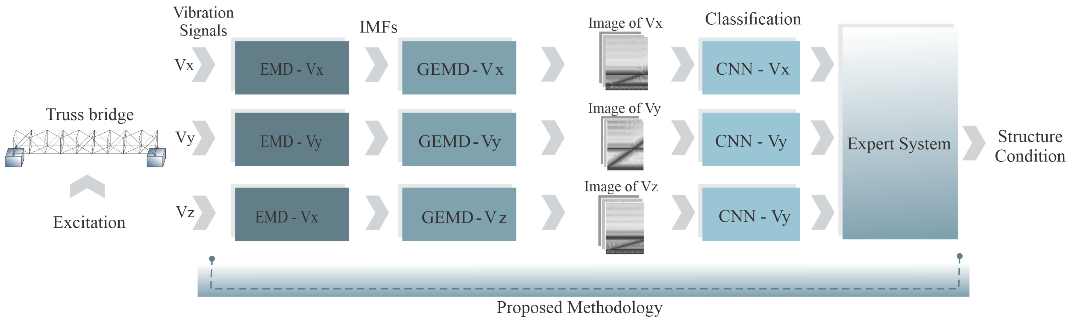
Figure 1 presents the sequence of steps followed in the proposed methodology to assess the condition of a truss-type structure configured as a bridge. The process is divided into four key stages, ensuring a comprehensive evaluation framework.

The first stage involves the acquisition of vibration signals monitored and acquired along the three axes of a triaxial accelerometer (Vx, Vy, Vz). These measurements are taken under four structural conditions: healthy (intact members) and three levels of corrosion-induced damage—incipient, moderate, and severe. The signals are obtained from a 3D nine-bay truss structure configured as a bridge, which is excited using a low-amplitude dynamic input, comparable to ambient vibrations, applied through an electrodynamic shaker [44].

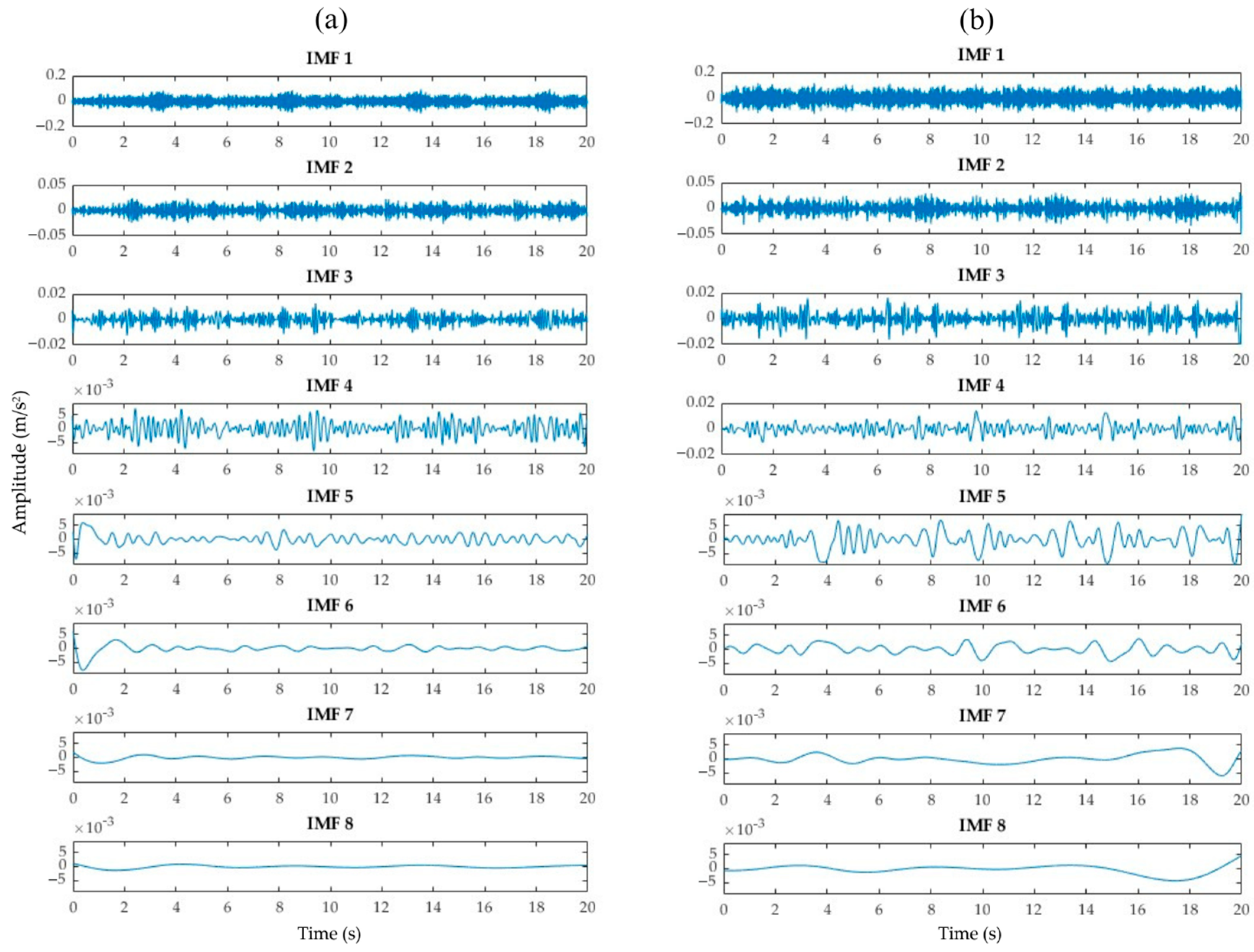
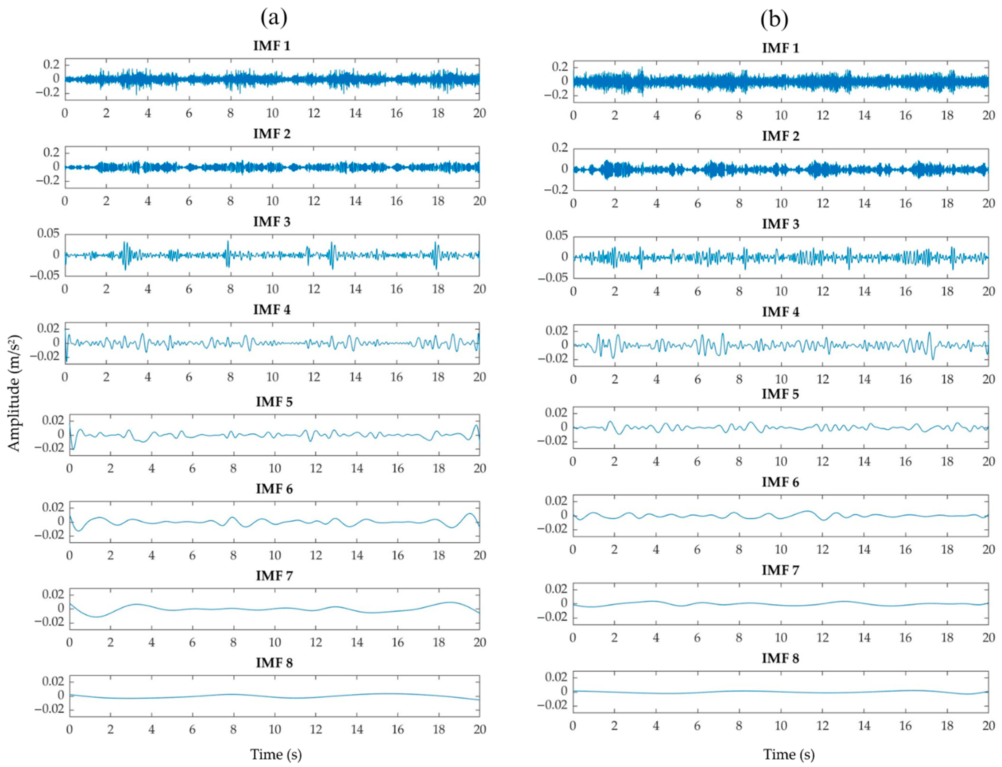
In the second stage, each of the acquired vibration signals (one per axis) is processed using GEMD. In particular, this technique decomposes the signals into their intrinsic mode functions (IMFs) or frequency bands, enabling the identification of features associated with the structural condition. From these IMFs, time–frequency representations are generated for each axis, which are subsequently converted into grayscale images. These images serve as input for the next stage.

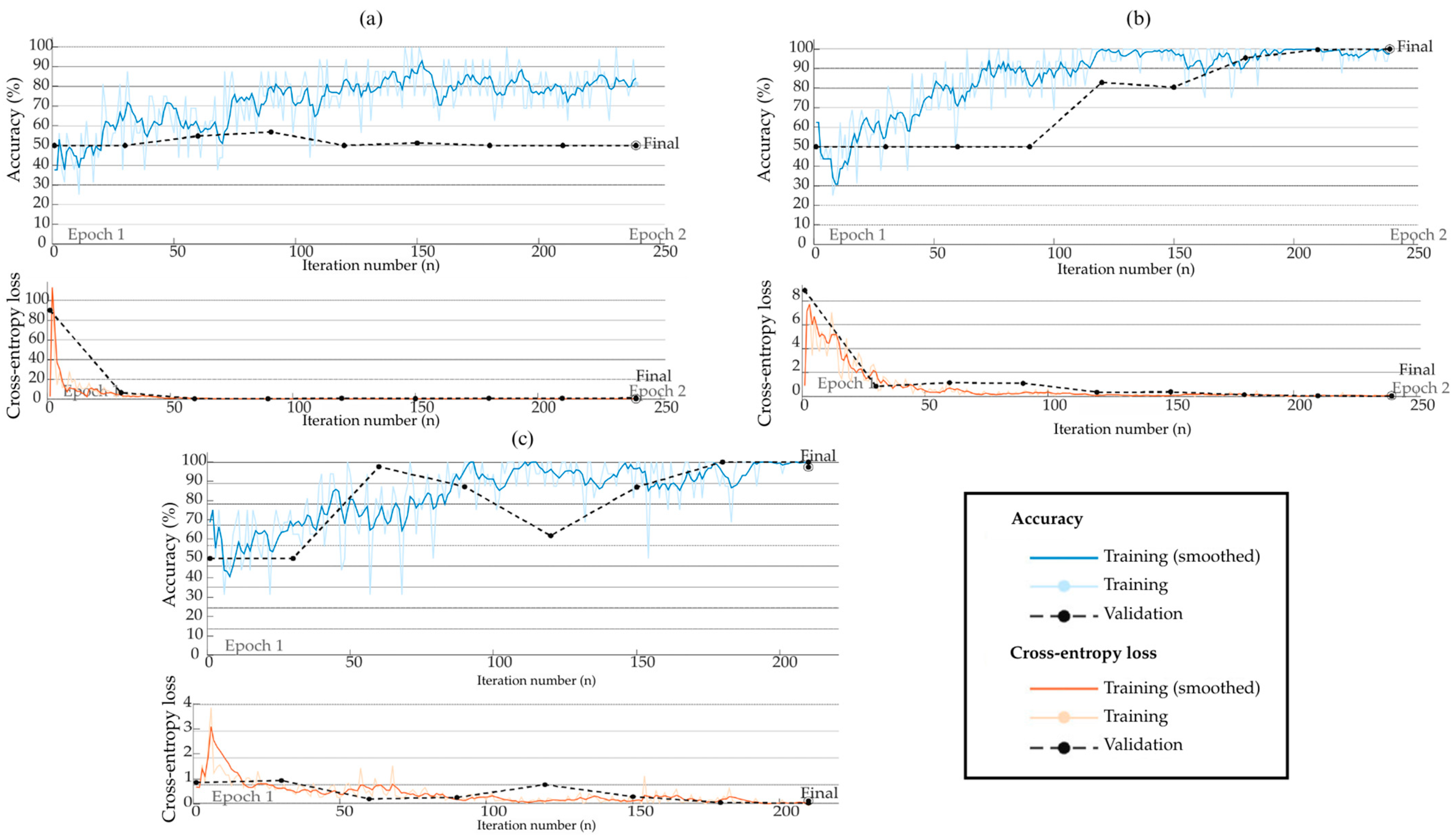
The third stage corresponds to pattern recognition, where a dedicated CNN is trained for each axis (one CNN for Vx, one for Vy, and one for Vz). Each CNN performs automatic classification, determining whether the corresponding axis reflects a healthy condition or one of the three levels of corrosion damage. It is important to highlight that the time–frequency images obtained from the GEMD decomposition are treated as conventional 2D images, enabling the use of 2D CNN architectures. During this stage, different configurations for image resolution, learning rate, and network depth are analyzed to optimize classification performance.

Finally, the fourth stage focuses on decision fusion, where an expert system evaluates the individual results provided by the three CNNs (one per axis). The expert system applies a set of if-else rules, designed to consolidate the classifications into a final diagnosis. These rules account for cases where all three axes agree, as well as cases where discrepancies exist between axes, ensuring a balanced interpretation that considers the possible anisotropic response of the structure to corrosion damage.

2.1. Graphical Empirical Mode Decomposition

Huang et al. [40] developed the EMD method, which has become a widely adopted approach for studying signals with nonlinear and non-stationary characteristics. Its primary function is to decompose a given signal into a set of components known as IMFs, each representing a different frequency band present in the original signal. For a component to be classified as an IMF, it must satisfy two fundamental conditions:

(a)

The number of zero crossings and extrema should either be equal or differ by no more than one.

(b)

At every point in the signal, the mean value of the lower and upper envelopes has to be approximately zero.

The extraction of each IMF is performed through an iterative procedure known as the sifting process, which follows these four steps:

• Detection of extrema and construction of envelopes.
  • The local maxima and minima of the signal x(t) are identified.
  • Employing the identified points, the lower envelope e_min(t) and the upper envelope e_max(t) are constructed through an interpolation, i.e., a spline interpolation. In this work, a cubic spline interpolation is employed because it provides smooth envelope curves, which can provide a suitable tracking of the oscillatory modes of the signal [40].
• Computation and subtraction of the mean envelope.
  • The mean of both envelopes is computed to obtain the local trend of the signal:

    $$m(t)={\displaystyle \frac{e_{\max }(t)+e_{\min }(t)}{2}}$$

    (1)
  • The obtained mean is then subtracted from the original signal to produce the first IMF candidate:

    $$h(t)=x(t)-m(t)$$

    (2)
• Verification of IMF conditions.
  • The function h(t) is evaluated to determine whether it satisfies the criteria (a) and (b).
  • If both conditions are met, the function h(t) is designated as the first IMF:

    $$c_1(t)=h(t)$$

    (3)
  • Otherwise, steps 1–2 are repeated until the function meets the required conditions.
• Computation of the residual and extraction of additional IMFs.
  • Once the first IMF is extracted, the residual is computed by subtracting it from the original time series signal:

    $$r_1(t)=x(t)-c_1(t)$$

    (4)
  • The resulting residual is considered a new signal, and the process is iteratively repeated to extract additional IMFs, denoted by c₂(t), c₃(t), …, until the final residual r_N(t), which is considered a monotonic function.

Once all IMFs are extracted, the original signal can be expressed as the sum of these components along with a residual term that captures the low-frequency trends of the data:

$$x(t)={\displaystyle \sum _{n=1}^N{c}_n(t)+r_N(t)}$$

(5)

Given its ability to handle signals with high variability and noise, the EMD method can be a suitable tool in vibration-based SHM, particularly for analyzing structures subjected to complex dynamic conditions.

Although the IMFs obtained through EMD can provide valuable insights into the structural condition of a civil infrastructure, their direct use in structural health evaluation is subject to expert analysis. Typically, only a subset of the extracted IMFs is selected based on specific frequency characteristics and their relevance to the damage detection process. This selection often requires a meticulous manual inspection to ensure that only the most informative IMFs are used, preventing the inclusion of noise-dominated or redundant components; however, this action does not guarantee that the selected information contains reliable information, especially when the reliable features present slight changes.

In contrast to conventional IMF selection approaches, this study considers that all extracted IMFs contain valuable information for an automated DL framework. Instead of manually selecting specific IMFs, the entire set is utilized to generate an image representation that serves as input for a CNN-based classification system. This approach eliminates the dependency on expert intervention and enables an end-to-end data-driven analysis.

To achieve this transformation, the GEMD technique is employed in this work. This technique converts the set of IMFs into a grayscale image representation through the following steps, which are described below and illustrated in Figure 2:

• The IMFs extracted from the EMD process are arranged to form a 3D surface plot, where the X-axis represents time, the Y-axis corresponds to the IMF index, and the Z-axis indicates the amplitude.
• The resulting surface is visualized from a top-down perspective, effectively projecting the IMF characteristics onto a 2D grayscale image.
• The grayscale intensity of the image encodes variations in IMF amplitude, preserving information about signal dynamics.
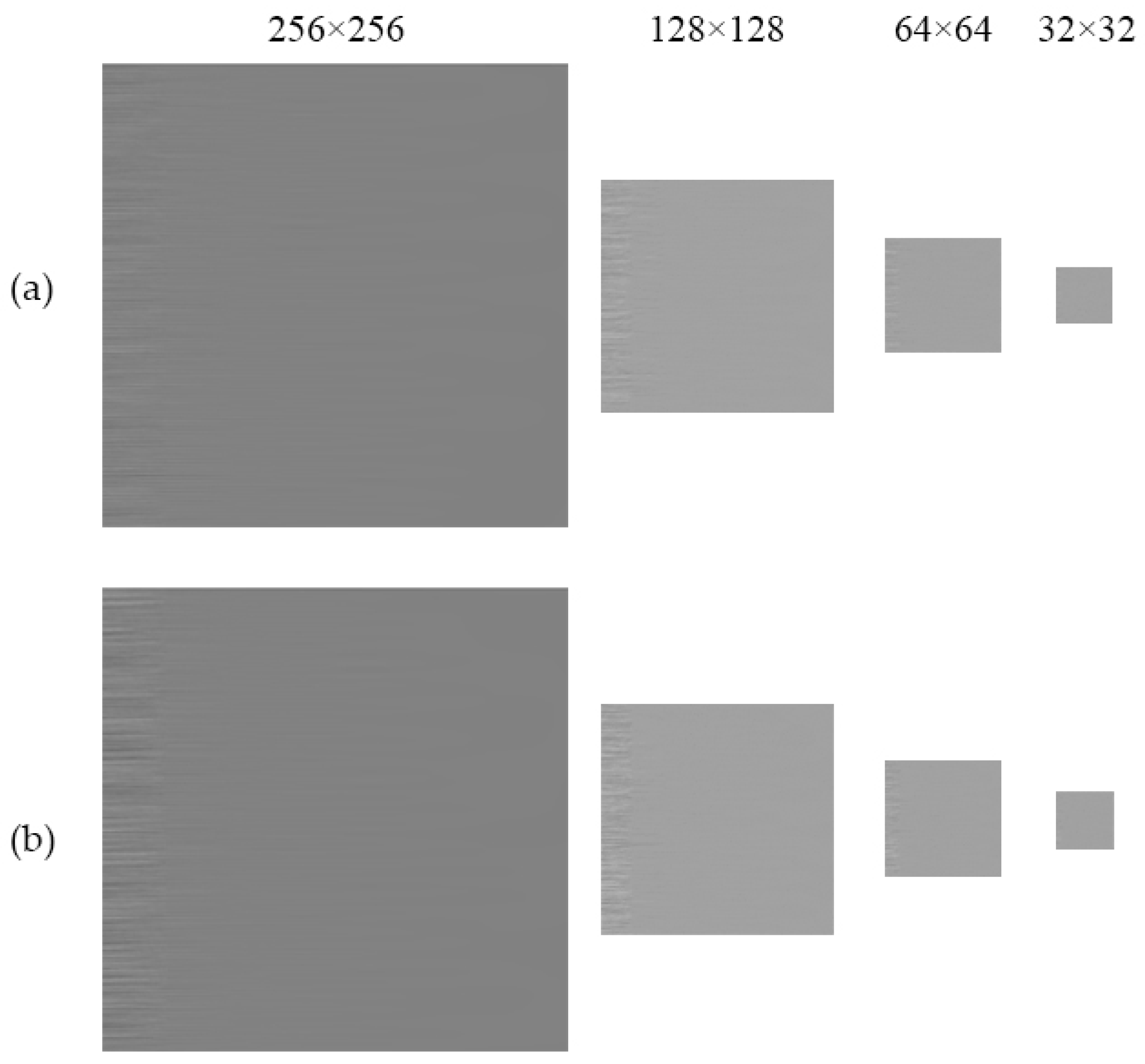
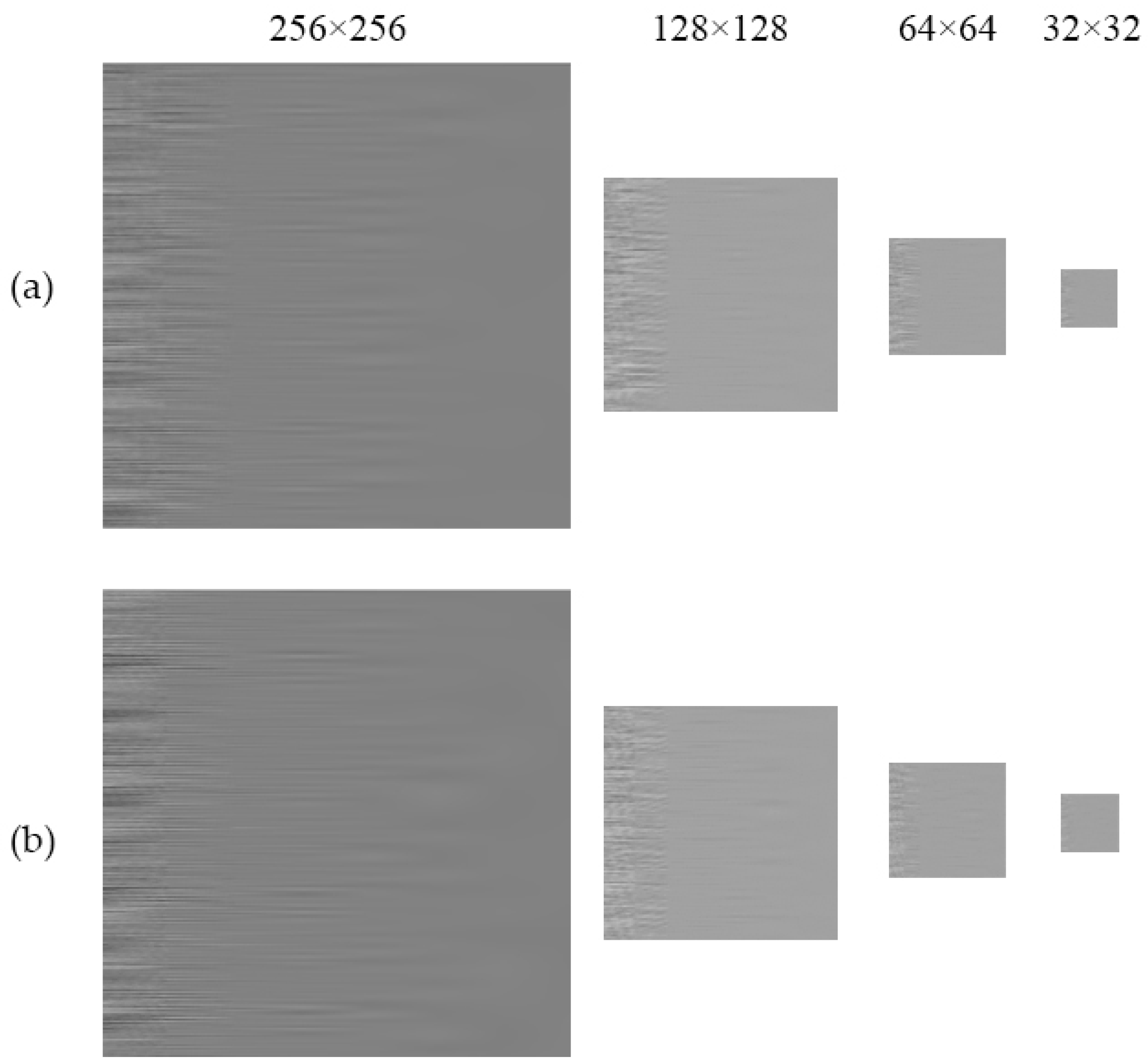
• The final image is resized to a fixed resolution (e.g., 256 × 256 pixels) to standardize the input format for the CNN model.

This image-based representation of IMFs enables CNNs to automatically learn patterns and extract meaningful structural health indicators without requiring predefined feature engineering. As a result, the proposed methodology enhances the efficiency and robustness of vibration-based SHM, particularly for identifying early-stage damage in civil structures.

2.2. Convolutional Neural Network

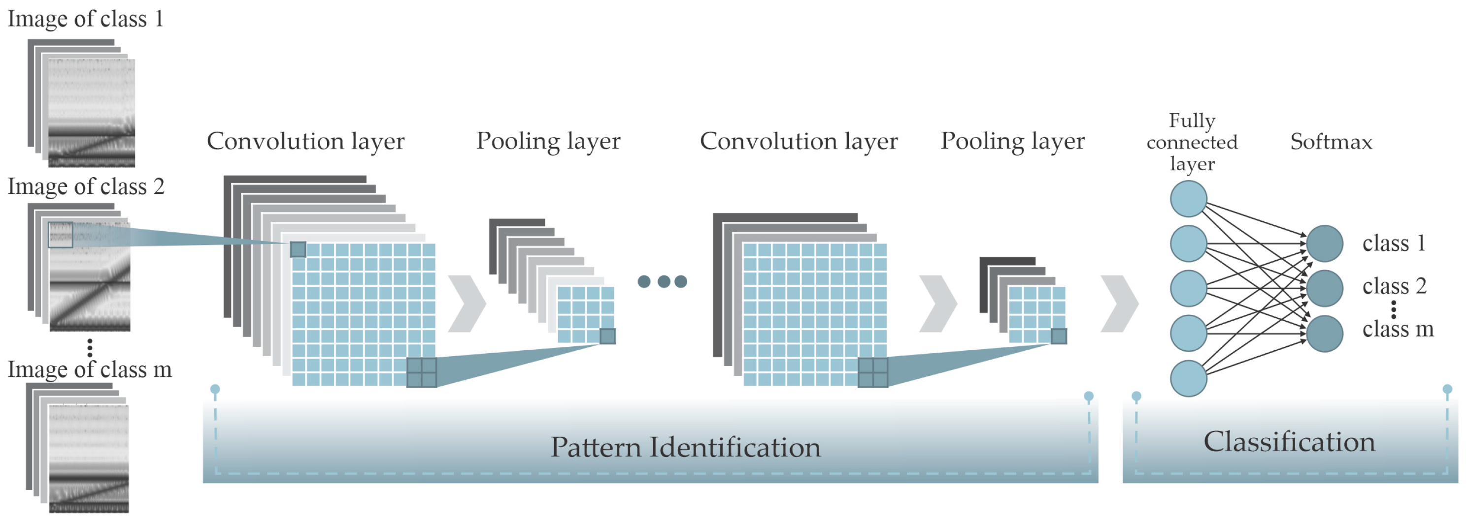
CNNs represent an innovative DL approach that is particularly effective for pattern recognition in images and time signals. Unlike other processing methods, CNNs integrate feature extraction and classification within a single learning framework, enabling automatic pattern identification in one-dimensional signals or images without requiring manual feature engineering during preprocessing and testing [45]. In particular, a CNN is composed of four fundamental layer types: convolutional, pooling, fully connected, and SoftMax layers (see Figure 3). Each of these layers serves a distinct function in the data processing pipeline [46].

In the initial stage, the input image, denoted as Ij with dimensions h × ω, undergoes a convolution operation, *, using a set of filters F_i, referred to as convolutional filters. This operation detects specific patterns within the analyzed image and follows the equation:

$$y_i=\sigma \left({\displaystyle \sum F_i^{\ast }{X}_j}+B_i\right)$$

(6)

where σ(⋅) represents a nonlinear activation function and B is a bias term. Each filter F_i, of size k₁ × k₂, is applied to local regions of the input image using a stride parameter s₁. The resulting feature maps y_i with dimensions z₁ × z₂, are computed as follows:

$$z_1={\displaystyle \frac{h-k_1+2p}{s_1}}+1$$

(7)

$$z_2={\displaystyle \frac{\omega -k_2+2p}{s_1}}+1$$

(8)

To maintain spatial resolution between the input and output, a zero-padding parameter P is introduced, typically set to 1 [47]. Among the various nonlinear activation functions used in neural networks, i.e., sigmoid, hyperbolic tangent, rectified linear unit (ReLU), exponential linear unit, among others, the ReLU, defined as f(y_i) = max(0, y_i), is the most commonly used in CNNs due to its efficiency in identifying nonlinear features [48].

After the convolutional stage, the feature maps are processed by the pooling layer, which reduces data dimensionality while preserving critical information for subsequent layers. This is achieved using filters of size K₁ × K₂ with stride s₂, which apply either max pooling (selecting the maximum value) or average pooling (computing the mean value) over selected regions. This process produces a condensed representation of y_i with dimensions Z₁ × Z₂, as given by

$$Z_1={\displaystyle \frac{z_1-K_1}{s_2}}+1$$

(9)

$$Z_2={\displaystyle \frac{z_2-K_2}{s_2}}+1$$

(10)

Both max pooling and average pooling help capture invariant patterns and enhance the generalization capability of CNNs. However, max pooling has shown superior performance, as it more effectively preserves invariant features and improves generalization [49]. Therefore, this study focuses on evaluating max pooling.

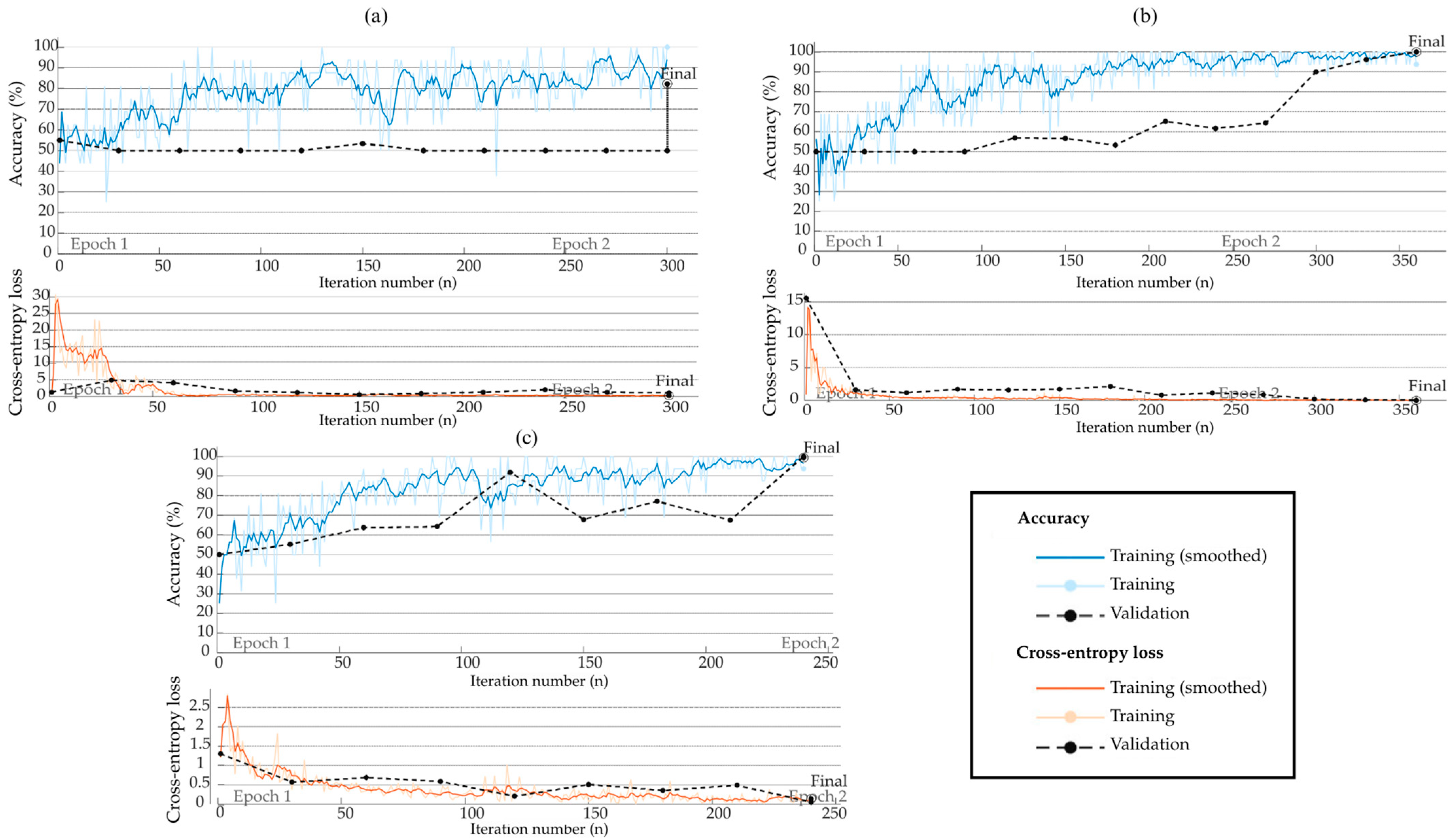
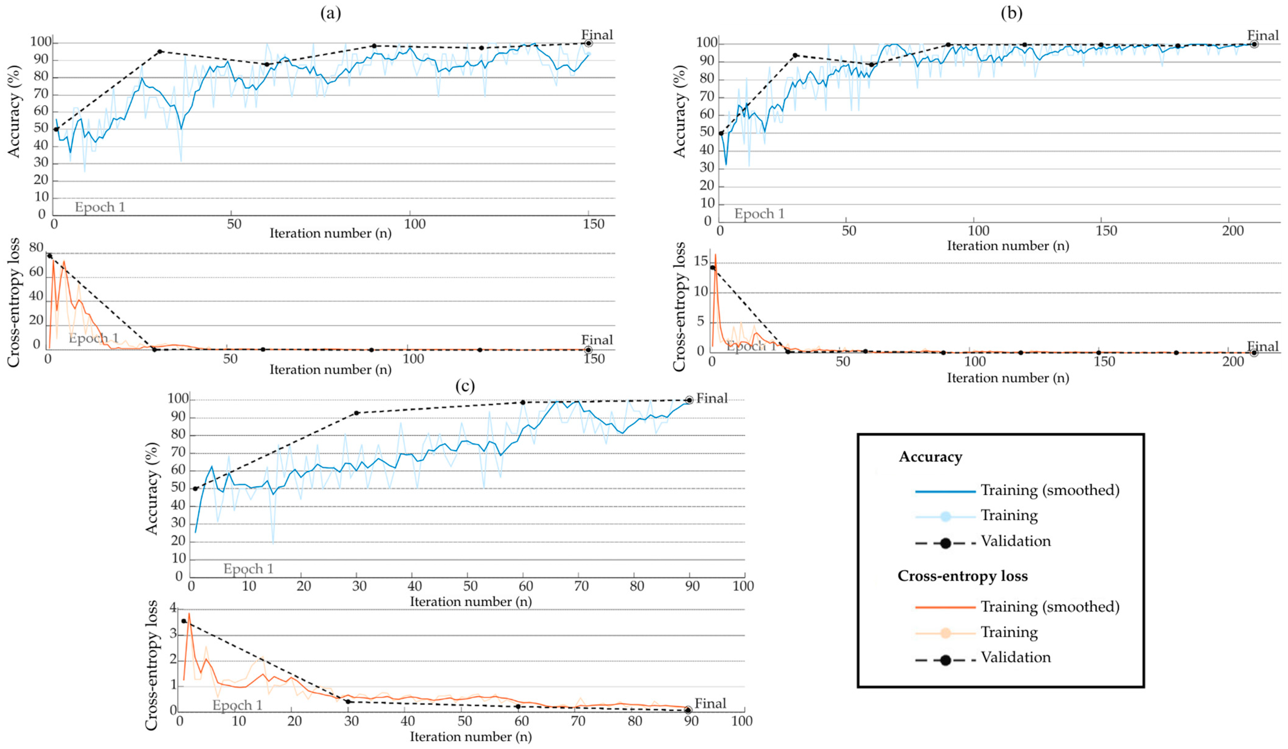
The features extracted from the previous layers are then passed to the fully connected layer, which functions as a traditional artificial neural network, such as a multilayer perceptron, for pattern recognition. Finally, the SoftMax layer generates the network’s output using a SoftMax transfer function. In this study, this final layer is employed to evaluate the truss bridge condition. In order to keep the computational complexity of the CNN low, four key factors are analyzed: (1) image size, (2) number of layers, (3) number of filters, and (4) filter size. Additionally, the initial learning rate is also considered, as it influences the training dynamics and computational requirements of the model.

2.3. Rules of Expert System

In particular, this work presents an expert system for SHM, designed to assess the condition of a truss bridge based on vibration signal analysis. The system utilizes a triaxial accelerometer to capture structural responses, with each axis independently analyzed using the GEMD-CNNs. The final classification is determined by a set of decision rules, ensuring a structured and reliable evaluation. The approach assumes that structural damage can affect multiple vibration axes; hence, in order to enhance accuracy, the expert system follows these proposed rules:

❖

Rule 1: Consistent structural condition.

• When all three CNNs detect damage, the expert system classifies the structure as damaged and recommends a detailed inspection to assess the severity.
• When all three CNNs classify the structure as healthy, the system determines that no damage is present.

❖

Rule 2: Predominantly damaged condition.

• When two CNNs indicate damage and one classifies the structure as healthy, the expert system suggests that damage is likely and advises repeating the analysis to confirm the diagnosis, since structural damage does not always affect all vibration axes equally. However, if two axes exhibit abnormal patterns, there is a high probability of structural deterioration.

❖

Rule 3: Predominantly healthy condition.

• When two CNNs classify the structure as healthy and one detects damage, the expert system does not rule out the possibility of deterioration, as the structure could present a very low level of damage, one that is subtle enough to go unnoticed in certain vibration components but might still be the first sign of a progressive failure process. In such cases, the system recommends conducting further analysis to track the possible evolution of the condition.

It is important to mention that the proposed expert system integrates multi-axis vibration analysis and DL classification to evaluate structural integrity. By applying predefined decision rules, the system improves reliability in damage detection, ensuring that inconclusive results prompt further investigation rather than leading to uncertain assessments. This methodology supports early-stage SHM, facilitating proactive maintenance and long-term infrastructure safety.

3. Experimental Setup

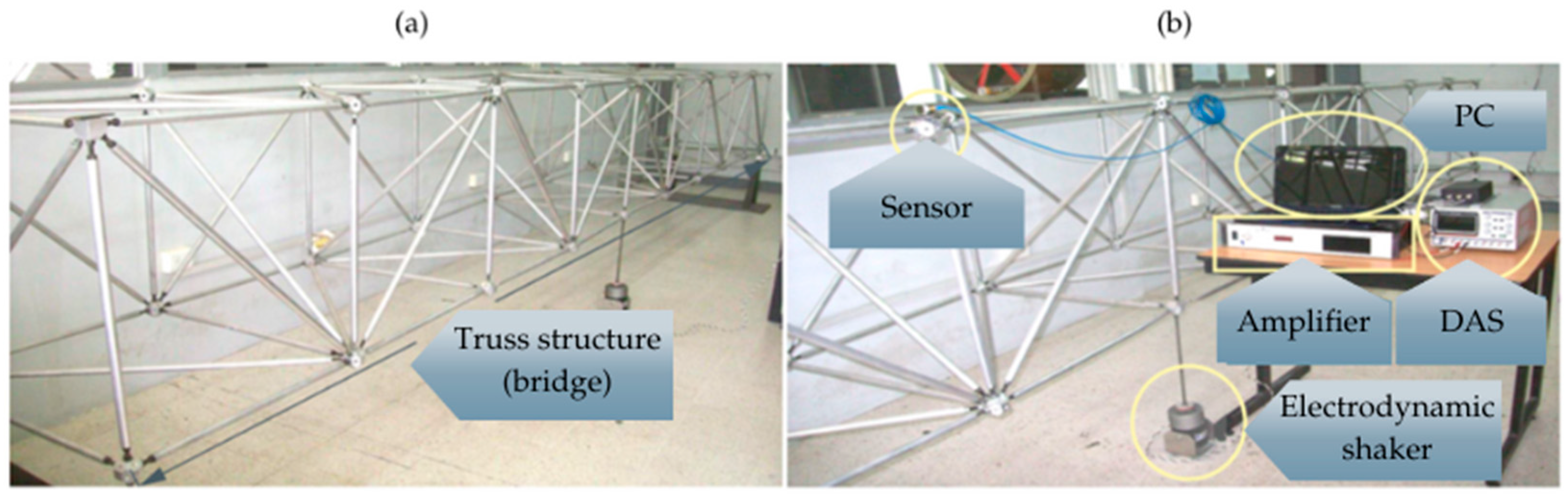
The experimental setup designed to assess the structural integrity of the analyzed truss structure is shown in Figure 4. This setup is located at the Autonomous University of Queretaro, Campus San Juan del Rio, Mexico. The structure consists of a modular truss structure configured as a bridge, composed of nine cubic or bay elements, forming a framework that allows for controlled damage analysis. The structure is constructed from 6061-T6 aluminum alloy, which contains approximately 0.8–1.2% of magnesium, 95–98% of aluminum, 0.15–0.40% of copper, and 0.4–0.8% of silicon [50]. It has an overall length of 6.40 m, with a height and width of 0.71 m each. The individual bars forming the truss have a diameter of 19 mm, while the horizontal and vertical members measure 0.70 m in length. The diagonal bars extend to a length of 0.70√2 m, providing stiffness, stability, and ensuring a robust structural configuration (see Figure 4a). Additionally, it is important to mention that the design and construction of the bridge used in this work were inspired by the truss-type bridge proposed by [51], adapted to the available infrastructure, and this structure shares similarities with other truss bridge models reported in the literature, making it a representative benchmark for experimental damage detection studies [52].

To induce vibrations into the bridge, an electrodynamic shaker (Labworks model ET-126B, Labworks Inc, Costa Mesa, CA, USA) was used along with a linear amplifier (Labworks model PA-138, Labworks Inc, Costa Mesa, CA, USA), generating continuous low-intensity and low-frequency dynamic excitations (see Figure 4b). Considering the bridge longitudinal direction, the shaker was positioned near the mid-span between the supports of the structure; whereas taking into account the transverse direction, the shaker was located on one of the sides of the bridge instead of the center. This strategic shaker position, together with the established border conditions, allowed the generation of the highest possible vibration amplitudes in all 3 axes at the same time, due to the structural dynamics of the truss. Placing the shaker in this position ensures a more uniform energy distribution across the bridge and maximizes the amount of vibrational data collected, enhancing the effectiveness of the damage detection analysis [53]. Thus, the vibration responses of the structure were generated using white Gaussian noise with a frequency bandwidth of 0 Hz to 100 Hz, covering the entire frequency range of interest.

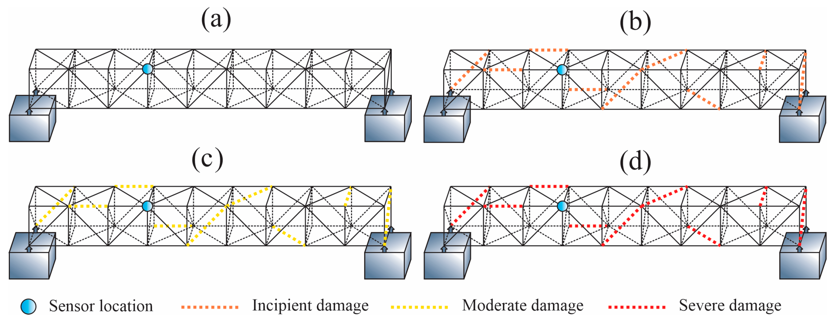
The dynamic behavior of the structure was monitored using a Kistler triaxial accelerometer (model 8395A; Kistler Group in Winterthur, Switzerland) with measurement axes Vx, Vy, and Vz. This sensor features a ±10 g measurement range, a resolution of 400 mV/g, and an operational bandwidth of 0–1000 Hz. The monitored data were collected through a National Instruments data acquisition system (model NI USB-6002; Austin, TX, USA), which includes a 16-bit analog-to-digital converter. Since structural damage propagates across multiple points, this study focuses on data collected from the sensor positioned at bay 4, as shown in Figure 5. This specific location was chosen because it corresponds to the central region of the structure, where vibration amplitudes are expected to be higher, ensuring a more pronounced response to damage-induced variations. Placing the sensor in this area provides more useful information about the dynamic behavior of the bridge, as the ends tend to show lower displacements and thus offer limited data. Hence, monitoring the central region improves data acquisition by capturing subtle changes in the structure’s dynamic response that may indicate the presence and progression of damage [54].

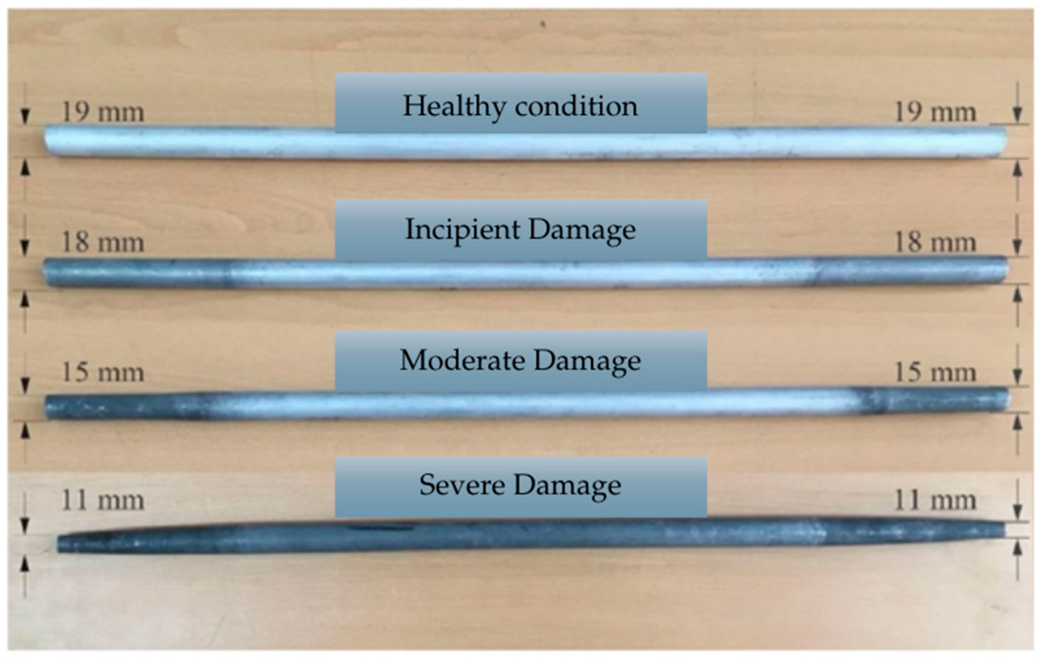
To simulate different structural damage scenarios, controlled tests are conducted by introducing bar elements affected by corrosion into the truss-type bridge. Three corrosion levels—incipient, moderate, and severe—are induced, reducing the bar diameters by 1 mm (see Figure 5b), 4 mm (see Figure 5c), and 8 mm (see Figure 5d), respectively. The sampling frequency was set at 200 Hz for each test, with each trial lasting 20 s, resulting in 4000 recorded samples. For each damaged cube, 300 tests were obtained, distributed as 100 for incipient damage, 100 for moderate damage, and 100 for severe damage. Considering all damage levels across all cubes, this results in a total of 2700 datasets for damaged conditions. Additionally, 2700 datasets were obtained for the healthy condition, leading to a total of 5400 experiments. Given that a separate CNN is employed for each axis, the final dataset comprehensively covers both undamaged and damaged conditions with balanced representation. For each bay, the selection of the damaged element was randomized to assess the robustness of the proposed damage detection methodology, regardless of the damage location. This randomized approach ensured that different structural elements were affected throughout the experiment. It is important to highlight that, throughout the experiments, the damage was introduced sequentially across the structure. Initially, the damaged element was placed in the first bay while the rest of the structure was intact. For example, in one test sequence, damage was first introduced in a diagonal bar of the first bay (Figure 5b). Then, the damage was relocated to the second bay, restoring the first to its undamaged state, while the other bays stayed unaffected. This approach allowed for a systematic evaluation of the structure’s response to localized defects, enhancing the reliability of the proposed damage detection methodology.

Damaged Elements

Since natural corrosion is a slow process [55], an accelerated approach was implemented to evaluate its effects on the structural behavior of the experimental truss. To induce controlled external corrosion, the ends of aluminum bars were immersed in hydrochloric acid, leading to progressive material loss. The undamaged bars have a diameter of 19 mm and a mass of 445 gr. After corrosion, the bars exhibited diameter reductions of 1 mm, 4 mm, and 8 mm at their extremities, corresponding to incipient, moderate, and severe damage levels, respectively. These reductions were associated with mass losses of 19.7 gr, 49.7 gr, and 84.4 gr relative to the intact element. The selected damage levels ensured that the structural integrity of the bars was maintained throughout the experiment, allowing for a controlled yet realistic representation of material degradation [50]. Figure 6 illustrates the different corrosion conditions, including an intact bar and those with varying degrees of deterioration or corrosion. It is important to mention that the corrosion was induced only at the bars’ ends in order to represent damage scenarios in the most critical parts of the truss-type bridge (zones of bars’ ends/joints), which are considered as stress concentrators regions where the bridge will tend to fail first due to the degradation of those elements. In this way, we generated realistic damage cases where corrosion may begin at the bars’ ends and, consequently, the proposed methodology was validated under more rigorous conditions; that is, the method was applied to detect damage where corrosion reduced the diameter of the bars only at the ends rather than throughout the entire bars.

4. Results

4.1. Signal Decomposition

The vibration signals used in this study were acquired using a triaxial accelerometer positioned at bay 4 of the truss-type bridge structure. This central location was selected because it tends to exhibit the highest amplitude responses due to the dynamic behavior of the system, thus maximizing sensitivity to damage-induced variations [53]. The structure was evaluated under four different conditions: healthy and with incipient, moderate, and severe corrosion. Damage was introduced in one bay at a time to allow controlled analysis of each scenario, as described in Section 3.

Once acquired, the vibration signals corresponding to each axis, Vx, Vy, and Vz, were preprocessed using EMD, which decomposes each signal into a set of IMFs representing distinct frequency components. To ensure consistency in the image representations used for subsequent CNN classification, the number of IMFs was fixed at eight, as this was the minimum number consistently obtained across all signals during the experimental trials. This standardization helps prevent variability in the image-based inputs, ensuring uniform feature extraction during the classification process. Figure 7, Figure 8 and Figure 9 illustrate representative examples of the IMF decomposition for each vibration axis. These comparisons show the signal from a healthy structure alongside signals with severe corrosion, all corresponding to damage introduced in bay 9, the farthest location from the sensor. This scenario was selected because it represents a more challenging detection condition due to the increased distance from the sensing point. Although slight variations can be identified across the obtained IMFs, these differences are neither pronounced nor easily distinguishable through visual inspection alone. This limitation emphasizes the importance of employing a more robust analysis strategy. Rather than interpreting each IMF individually, this study proposes the GEMD approach, described in Section 2.1, to combine all IMFs into a single grayscale image that encapsulates the time–frequency characteristics of the original signal. This unified image serves as input to the CNNs, enabling the automated extraction of subtle patterns that would otherwise remain hidden. By leveraging the CNN’s capacity to learn complex representations, the system enhances the reliability and accuracy of structural condition classification.

4.2. CNN Performance Evaluation and Expert System

To evaluate the capabilities of CNN to discover suitable features in order to distinguish between a healthy and a damaged condition, it is trained using grayscale images of 256 × 256 pixels, obtained through the GEMD process for the three vibration axes. This image resolution was selected because it allows preserving fine details from the signal transformation while maintaining a manageable computational cost [56]. It is essential to mention that the data are balanced for each axis, comprising 2700 healthy and 2700 corroded images (900 samples for each corrosion severity level: incipient, moderate, and severe). Subsequently, the dataset was randomly divided into 70% for training, 20% for validation, and 10% for testing. This division ensured established practices for large balanced datasets, where single random splits provide statistical reliability when combined with regularization techniques [57]. On the other hand, a 40% dropout rate was applied in fully connected layers [38], disrupting neuronal co-adaptations to mitigate overfitting and enhance generalization [58]. The model’s consistently high accuracy (>99% across all axes) and stable loss convergence further validate this approach.

During the experiment, CNNs with one to three convolutional blocks were tested in order to evaluate classification performance. To determine the appropriate depth for the CNN, architectures with one to three convolutional blocks were evaluated to analyze their classification accuracy. This range was selected to strike a balance between feature extraction capability and computational cost. Increasing the depth beyond three blocks typically results in diminishing returns, while increasing the risk of overfitting and processing time without improving performance [59]. Therefore, three blocks were set as an upper limit for the complexity of the proposed model. In this regard, it is important to mention that the CNN with one convolutional block has a 2D convolutional layer, which includes 256 filters with a 3 × 3 kernel size, where the same padding to preserve spatial dimensions is employed. The choice of 3 × 3 kernels was motivated by two key factors: (1) smaller kernels are more effective in capturing high-frequency damage signatures, such as abrupt changes in IMF amplitudes, than larger filters, as observed by [39], and (2) they offer greater computational efficiency, requiring nine times fewer parameters than 5 × 5 filters while achieving comparable receptive fields when stacked, consistent with the findings in [46]. This layer was followed by a batch normalization to stabilize training, a ReLU activation function for nonlinearity, and a max-pooling layer with a stride of 2 to reduce the feature map size. On the other hand, the CNN with two convolutional blocks has the same configuration as the previously investigated CNN, but the first convolutional block has 128 filters and the second block has 256 filters. Finally, the CNN with three convolutional blocks has the same configuration as the CNN with one convolutional block. Still, the convolutional blocks have 256, 128, and 64 filters for the first, second, and third convolutional blocks, respectively. All CNNs tested (one, two, three convolutional blocks) in this final part have a fully connected dense layer with 256 neurons added, preceding the SoftMax output layer with two neurons, responsible for binary classification (healthy or corroded). The model was trained using the Adam optimizer with a learning rate of 0.001, which ensured stable training and avoided oscillations observed with higher learning rates (n > 0.01) [44]. A dropout rate of 40% was applied, as suggested by [38]. It is important to note that the selection of hyperparameters, such as the learning rate and dropout rate, was guided by empirical testing and insights from the related literature [38,44,57,58]. A learning rate of 0.001 was chosen because higher values led to unstable training behavior. A dropout rate of 40% was achieved following recommendations from similar studies, helping to reduce overfitting without degrading performance. Although it did not apply formal search methods like grid search or Bayesian optimization, exploratory experiments confirmed that the selected values offered a good trade-off between stability, accuracy, and computational cost.

Figure 10, Figure 11 and Figure 12 show the obtained results of CNNs with one, two, and three convolutional blocks. In particular, these figures show the loss and accuracy curves obtained during the training process for each axis. It is crucial to mention that all reported performance metrics refer exclusively to the independent test set to ensure a robust evaluation of the model’s generalization capability. These plots provide insight into each configuration’s convergence behavior and classification consistency. This helps evaluate the CNN’s capability of learning relevant features for classifying structural integrity from high-resolution images. In particular, the loss curves correspond to the cross-entropy loss function, which is widely used for binary classification problems and is dimensionless; therefore, no physical units are included on the vertical axis. The x-axis indicates the iteration number, ranging from n = 0 to i iterations. Additionally, the Adam optimizer was employed to update the model weights during training due to its efficiency and adaptive learning rate properties. According to these figures, it can be observed that when a single layer with 256 neurons is selected (see Figure 10a and Figure 12a), the CNN’s accuracy decreased significantly, limiting its capability of distinguishing between the two conditions. On the other hand, the configuration of two and three convolutional blocks presents similar results. Therefore, a two-convolution-block configuration is chosen to preserve the ability to detect fine details in the evaluated images, while maintaining a convenient computational cost and adequate accuracy.

Figure 13 shows the confusion matrix for the CNN with two convolutional blocks. It can be observed that it has 100% accuracy in differentiating between healthy and corrosion conditions, regardless of the level of corrosion and location.

As mentioned previously, the image size 256 × 256 is evaluated, where suitable results are obtained in order to differentiate between the conditions. Subsequently, to reduce the computational load (the number of operations) associated with the input image size, the analyzed 256 × 256 image was resized to several smaller resolutions: 128 × 128, 64 × 64, and 32 × 32 pixels. It is important to mention that larger resolutions, i.e., 868 × 686 (original image size) and 512 × 512, yielded 100% accuracy. Only for exemplification, Figure 14, Figure 15 and Figure 16 illustrate the different image dimensions to be used, both for a healthy and an incipient corrosion signal, for each axis. Therefore, these new image sizes are employed to train the CNNs and investigate their performance.

To evaluate the performance and computational efficiency of the proposed CNN architecture, multiple configurations were tested by varying three key parameters: the number of filters in the first and second convolutional layers, the number of neurons in the fully connected layer, and the input image resolution. For the first convolutional block, three different amounts of filters were tested, i.e., 126, 64, and 32 filters. In the second computation block, 256, 128, and 64 filters were tested, and, finally, in the fully connected layer, 256, 128, and 64 filters were tested. On the other hand, the image sizes considered were 128 × 128, 64 × 64, and 32 × 32 pixels. Each CNN model includes two convolutional layers, and each of these is followed by a max pooling layer, which reduces the spatial dimensions of the feature maps while preserving key information for classification. The classification accuracy for each configuration was assessed across the three vibration axes, and the results are presented in

Table 1. Best accuracy for each CNN configuration under different image sizes.

Measurement Axis	Configurations			Image Size
	First Layer	Second Layer	Fully Connected	256 × 256	128 × 128	64 × 64	32 × 32
Vx	128	256	256	100%	100%	100%	50%
	64	128	128	100%	100%	100%	99.91%
	32	64	64	100%	100%	50%	50%
Vy	128	256	256	100%	87.59%	100%	67%
	64	128	128	100%	81.20%	99.80%	50%
	32	64	64	100%	99.07%	50%	50%
Vz	128	256	256	100%	100%	100%	99.9%
	64	128	128	100%	100%	98.89%	99.9%
	32	64	64	100%	100%	100%	100%

. To facilitate interpretation, a color-coding scheme was applied: gray highlights the original configuration, green highlights the configuration with the highest accuracy per image resolution, yellow indicates the most computationally efficient setup (using the lowest number of filters and neurons) that still achieved high performance, and red marks the configuration that consistently reached 100% accuracy across all three axes using the same architecture at the 64 × 64 resolution. The same CNN configuration was applied to all axes to ensure consistency and facilitate practical implementation. Therefore, in cases where an axis achieved slightly higher accuracy with a different setup (e.g., 67% on Vy), the result reported corresponds to the shared configuration across axes. This approach ensures compatibility, deployment uniformity, and the selection of robust architectures suitable for real-world SHM applications.

The unified evaluation confirms that high-resolution images, such as 256 × 256, allow the CNN to fully exploit the non-stationary patterns present in the IMFs. This results in perfect classification accuracy across all configurations, even for incipient damage levels. Conversely, the lower resolution of 32 × 32 pixels leads to significant information loss, with some configurations achieving only 50% accuracy due to insufficient detail for reliable feature extraction. Among the configurations tested, the one marked in red for 64 × 64 images (filters: 32 and 64; fully connected layer: 64 neurons) emerged as the most balanced option, offering 100% classification accuracy across all axes. In the first instance, the red configuration would be the best option; however, it must be verified that this configuration performs the fewest operations, which ultimately translates into the method’s computational load. This is to choose the best configuration for real-time and embedded SHM systems, where accuracy and efficiency are critical.

4.2.1. Selection of the Better Configuration

The number of floating-point operations (FLOPs) performed by each part of the CNN (i.e., the convolutional and output blocks) is also considered to select the best configuration. From the observations in Table 1, the highlighted configurations were chosen, that is, gray that corresponds with original configuration, i.e., image size 256 × 256 and 128 filters for the first layer, 256 filters for the second layer, and 256 filters for the fully connected layer named in

Table 2. CNN FLOPs for each configuration.

Section Where Operations Are Performed	Configuration
	A	B	C	D
First block	159,383,552	9,961,472	9,961,472	1,245,184
Second block	9,672,065,024	151,519,232	604,504,064	37,814,272
Output block	536,871,936	8,388,864	33,555,456	2,097,664
Total	10,368,320,512	169,869,568	648,020,992	41,157,120
Percentage of reduction	0.00	98.36	93.75	99.60

as “A”. Green that corresponds with a configuration of 32 filters for the first layer, 64 filters for the second layer, and 64 filters for the fully connected layer per image of 128 × 128 pixels called in Table 2 as “B”. The red color corresponded to the configuration by analyzing an imagen size of 64 × 64 with 128 filters for the first layer, 256 filters for the second layer, and 256 filters for the fully connected layer; in Table 2, it is known as “C”. Finally, the text highlighted in yellow correspond to the configuration of 64 filters for the first layer, 128 filters for the second layer, and 128 filters for the fully connected layer by an image of 32 × 32 pixels, which, in Table 2, is called “D”. Table 2 shows the FLOPs performed when analyzing each image, for each configuration, because these operations directly affect the computational load and time of processing.

Hence, considering the information presented in Table 1 and Table 2, the following information is obtained: configuration D (64 filters for the first layer, 128 filters for the second layer, and 128 filters for the fully connected layer per image of 32 × 32 pixels) has the highest FLOPs reduction; however, its ability to distinguish between states is the lowest, with 99.91% accuracy in Vx, 50.00% in Vy, and 99.90% in Vz. Configuration C (128 filters for the first layer, 256 filters for the second layer, and 256 filters for the fully connected layer per image of 64 × 64 pixels) has the highest ability to discern between states with 100% accuracy for Vx, Vy, and Vz; however, it is the configuration with the lowest FLOPs reduction. Configuration B (32 filters for the first layer, 64 filters for the second layer, and 64 filters for the fully connected layer per image of 128 × 128 pixels), highlighted in green, is chosen as the best configuration for the expert system. This is because in the three axes it presents accuracy results above 99%, which assures that the expert system will provide a good accuracy, also this configuration reduces the FLOPs by 98.36% compared to the first or original configuration proposed. Although the selection of the optimal configuration of a CNN should ideally be approached as a multi-objective optimization problem, a systematic exploration of the configurations was chosen in this work. This strategy allows for reducing computational complexity and finding an appropriate balance between computational time and model accuracy. Hence, the best selection of CNN configuration in this study was defined as the one that achieved the highest classification accuracy across all vibration axes while minimizing computational cost. The goal was to ensure feasibility for real-time or embedded SHM applications. To identify this configuration, the accuracy results and FLOPs were evaluated across various architectures, considering the number of filters, the fully connected layer size, and input image resolution. The configuration that reached 99% accuracy while reducing FLOPs by 98.36% (Configuration B) was selected as the most suitable CNN for this study.

4.2.2. Expert System for Corrosion Classification

Since each axis contributes independently to classification, a rule-based expert system is implemented to enhance robustness. This system integrates the CNN outputs of the selected configuration, B, i.e., 32 filters for the first layer, 64 filters for the second layer, and 64 filters for the fully connected layer per image of 128 × 128 pixels for the Vx, Vy, and Vz axes, applying the decision rules established in Section 2.3 to ensure a healthy and corrosion assessment without importing the level of corrosion. By incorporating these predefined rules, the expert system enhances reliability in corrosion detection, mitigating errors due to isolated misclassifications from individual CNNs, resulting in an accuracy of 100% in distinguishing between healthy and corroded conditions. It is essential to mention that the expert system was tested with 270 images for healthy and corroded conditions, respectively, corresponding to 10% of the total number of images available, which were selected randomly. This approach ensures that uncertain cases trigger further investigation rather than leading to ambiguous assessments, supporting early-stage structural health monitoring and proactive maintenance strategies. Figure 17 shows the confusion matrix of the expert system. In this case, it is observed that the system complements the information coming from each axis, since it avoids partial discrepancies and consistently detects between healthy and corroded (regardless of the corrosion level of the bar).

5. Discussion

The early detection of corrosion in civil structures, particularly in truss-type bridges, is crucial for preventing catastrophic failures that could compromise public safety and infrastructure integrity. In this context, the methodology proposed in this work, based on GEMD, CNNs, and a rule-based expert system, offers an innovative solution for identifying corrosion damage even at incipient stages, where vibrational signal alterations are minimal and difficult to detect using conventional methods.

One of the key contributions of this study is the integration of GEMD to transform vibration signals into graphical representations that preserve the NL and NS characteristics of IMFs. Unlike traditional approaches that require manual selection of relevant IMFs [26,40], the proposed method uses all IMFs to generate grayscale images, eliminating subjectivity in feature extraction and maximizing the information available for classification. This approach contrasts with previous works relying on techniques such as wavelet transforms [30], which, although effective, can be noise-sensitive and require extensive preprocessing. It is particularly important to note that several studies have been reported using the dataset introduced in this work, either partially or fully. For instance, in [28], a methodology based on fractality indices and a decision tree classifier was presented, achieving 100% accuracy. In [39], a method based on the autocorrelation of vibration signals and a one-dimensional CNN for signal classification was proposed, achieving an accuracy of over 97%. Finally, in [50], a methodology using fractality indices and autoencoders was developed, in which a new damage indicator was introduced, achieving 99.8% accuracy. Unlike the aforementioned works, although promising results were achieved, the proposed GEMD-CNN-based model, which also achieves 100% accuracy, does not require manual feature selection or extraction as in [28,50], enabling better generalization of the method. Furthermore, in the proposed model, the CNN architecture was improved, leading to a 98.36% reduction in computational load compared to the baseline model. This is in contrast to the CNN used in [39], which underwent no optimization process.

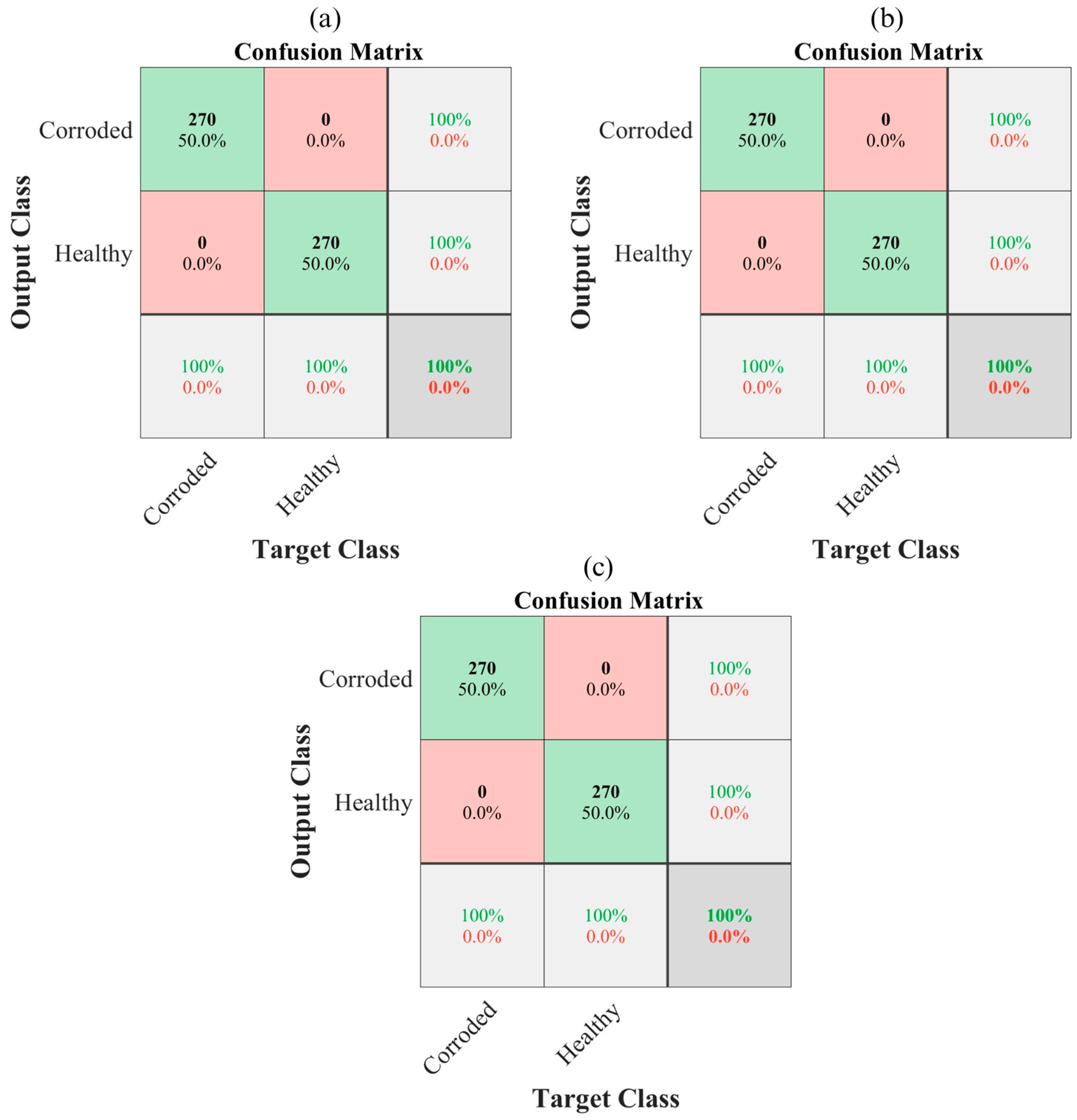
The proposed expert system significantly enhances the robustness of the damage detection framework by implementing intelligent decision rules that analyze multi-axis vibration data. While individual CNNs achieve high accuracy (100%) for each vibration axis, the expert system provides several critical advantages: (i) by implementing a voting mechanism across all three axes, the system can manage cases where damage affects vibration components asymmetrically (rules 2 and 3), reducing false positives/negatives that might occur with single-axis analysis; (ii) the rule-based approach provides clear criteria for damage assessment, making the results more interpretable for engineers; and (iii) the system’s ability to recommend follow-up actions (e.g., repeated analysis for borderline cases) enables early intervention before damage progresses.

Furthermore, the use of CNNs enables the automatic learning of complex patterns directly from GEMD-generated images, thereby overcoming the limitations of manual feature-based methods (e.g., Shannon’s entropy [32] or more complex solutions, such as fractals and autoencoders [50]). While recent studies have employed CNNs for damage detection [39,44], the proposal stands out due to the following. (i) Computational efficiency: The enhanced CNN architecture (reducing images to 128 × 128 pixels and minimizing filters) achieves 100% accuracy with a 98.36% reduction in floating-point operations. While comprehensive embedded system metrics (such as inference time and memory footprint) require future testing, this significant computational efficiency improvement suggests the method’s potential for implementation on low-cost embedded hardware in real-world monitoring applications. (ii) Robustness to damage location: unlike methods requiring multiple sensors [53], the proposed system uses a single triaxial accelerometer, demonstrating effectiveness regardless of corrosion location on the structure. (iii) Integrated decision making: The expert system combines multiple CNN outputs through logical rules, providing more reliable assessments than single-classifier approaches.

Despite promising results, this study has limitations that open avenues for future research. For instance, experiments were conducted on an aluminum bridge model under simulated ambient excitations; therefore, validation on real-world structures subjected to dynamic loads (traffic and wind, among others) and environmental conditions (humidity, temperature, etc.) is necessary [43]. In addition, although the GEMD-CNN methodology showed reliable performance in this study, the number of IMFs selected (eight) should be adjusted based on the specific conditions and characteristics of each structure in practical applications. While this study demonstrates the CNN’s computational efficiency through FLOPs reduction, two implementation challenges remain: (1) GEMD processing still requires substantial resources, and (2) practical deployment metrics are pending. Future work will focus on (1) embedded platform validation (Raspberry Pi/Jetson Nano) to measure real-time inference latency and memory usage, and (2) developing lightweight GEMD variants through techniques like fixed-point quantization or approximate computing. These steps will bridge the gap between laboratory validation and field-deployable SHM. The expert system rules could also be expanded to incorporate probabilistic confidence levels from each CNN, potentially improving sensitivity to incipient damage. Also, the methodology focused on corrosion, but extending it to detect cracks, loosened bolts, or fatigue may require CNN retraining, additional vibration axes, and adaptation of the expert system rules to accommodate different damage signatures.

6. Conclusions

Corrosion is a major concern for the safety and longevity of civil structures, making early detection essential. This work introduced an innovative expert system designed to automatically and reliably identify corrosion in truss-type bridges, even at very early stages. The proposal combines GEMD to transform vibration signals into images, with CNNs trained to distinguish between healthy and damaged structures. A set of decision rules, an expert system, was also integrated to deliver a final diagnosis based on the vibration data collected along three different axes.

The experimental results showed that the proposed expert system can accurately detect the initial stages of corrosion, achieving 100% classification accuracy, regardless of where the damage is located in the structure. It is worth mentioning that the expert system’s high performance was achieved through an exhaustive experimental process in which multiple CNN architectures and image resolutions were tested. This led to the selection of a compact network and reduced image size, ensuring both high accuracy and low computational demand, an essential feature for real-time SHM, especially in resource-constrained environments.

One of the main strengths of this approach is its simplicity and practicality. It requires only a single sensor to monitor the entire structure, avoids complex manual signal processing, and is robust to noise and subtle variations. These features make it a strong candidate for real-world SHM, helping ensure timely maintenance and extending the useful life of key infrastructure. Although the proposed methodology demonstrated excellent performance under controlled laboratory conditions, its validation on full-scale, real-world structures subjected to variable environmental and operational factors remains pending. Additionally, since the experimental scenarios focused on specific types and locations of corrosion, the system’s sensitivity to other damage types or sensor placement should be further investigated in future work. Moreover, a study to estimate the percentage of diameter reduction at which the bar element begins to lose load capacity and its structural integrity is compromised will be conducted, so that the damage levels due to corrosion selected for future experimental tests will be more representative of the real severity affecting both the bar element and the entire structure.