Adaptive Warning Thresholds for Dam Safety: A KDE-Based Approach ^†

Abstract

Dams are critical infrastructures that provide essential services such as water supply, hydroelectric power generation, and flood control. As many dams age, the risk of structural failure increases, making safety assurance more urgent than ever. Traditional monitoring systems typically employ predictive models—based on techniques such as the finite element method (FEM) or machine learning (ML)—to compare real-time data against expected performance. However, these models often rely on static warning thresholds, which fail to reflect the dynamic conditions affecting dam behavior, including fluctuating water levels, temperature variations, and extreme weather events. This study introduces an adaptive warning threshold methodology for dam safety based on kernel density estimation (KDE). The approach incorporates a boosted regression tree (BRT) model for predictive analysis, identifying influential variables such as reservoir levels and ambient temperatures. KDE is then used to estimate the density of historical data, allowing for dynamic calibration of warning thresholds. In regions of low data density—where prediction uncertainty is higher—the thresholds are widened to reduce false alarms, while in high-density regions, stricter thresholds are maintained to preserve sensitivity. The methodology was validated using data from an arch dam, demonstrating improved anomaly detection capabilities. It successfully reduced false positives in data-sparse conditions while maintaining high sensitivity to true anomalies in denser data regions. These results confirm that the proposed methodology successfully meets the goals of enhancing reliability and adaptability in dam safety monitoring. This adaptive framework offers a robust enhancement to dam safety monitoring systems, enabling more reliable detection of structural issues under variable operating conditions.

1. Introduction

Dams are essential infrastructures in global water management, serving numerous vital functions, from water supply for drinking, irrigation, and industrial purposes to flood control and hydroelectric power generation. Maintaining these structures is paramount to ensuring their safety, reliability, and longevity. The urgency of effective dam management is increasing as many dams worldwide approach the end of their intended service life, raising concerns about their structural integrity. A recent report by United Nations University [1] highlights the global challenge of ageing dams and underscores the need for enhanced research in safety monitoring and control. Furthermore, reports indicate that 63 dam failures were recorded between 1976 and 2000, with an additional 46 failures occurring before 1976 [2], illustrating the critical need for rigorous monitoring practices.

A dam’s response to acting loads depends on a number of factors, such as the dam typology and environmental conditions, as well as material properties and age [3,4]. Monitored response variables, including deformation, cracking, and seepage, among others, provide insights into the dam’s current condition [5]. These data are collected by instruments located on or within the dam structure, forming a critical part of ongoing safety assessments [6]. They enable the identification of early warning signs, allowing for proactive maintenance and failure prevention [7,8]. Predictive models play a key role in dam safety by comparing real-time data with expected performance, facilitating prompt detection of anomalies in dam behavior [9,10].

Predictive modeling can be based on numerical approaches, such as the finite element method (FEM), or on data-driven approaches, from simple multilinear regression (e.g., hydrostatic–seasonal–time (HST) [11]) to more sophisticated machine learning (ML) techniques, like support vector machines (SVMs) [12,13], neural networks (NNs), random forests (RFs), and boosted regression trees (BRTs) [14], among others [9].

Model predictions are typically used in combination with an allowable interval to define warning thresholds: an interval of acceptable response is defined, centered in the model prediction, so that if the observation falls inside, the behavior is considered healthy, but is potentially anomalous otherwise. Defining appropriate warning thresholds is key in dam safety, since they serve as a first line of defense for anomaly detection. However, establishing effective thresholds presents challenges, particularly under extreme load conditions, due to limitations in model accuracy. Typically, warning thresholds are defined based on the standard deviation of the residuals [15,16].

However, using constant thresholds for dam safety warnings presents several limitations, particularly given the complex and variable nature of dam behavior. A fixed threshold does not account for fluctuations in external factors, such as seasonal changes in water levels, temperature variations, or extreme weather events, all of which can significantly impact the dam response and the model accuracy. This is more acute when predictions are generated with some ML models, whose accuracy is more dependent on the quality and variety of historical data, being even less reliable when extrapolating, i.e., when predicting response in front-load values out of the historical range of variation.

Some new techniques have been explored for determining improved warning thresholds. Li et al. [17] proposed a model that combines M-estimation with confidence intervals to enhance anomaly detection reliability. In this approach, the threshold is set using a combination of a scale estimator (ST) derived from M-estimation and the confidence interval radius (D), with the threshold represented as 3ST + D. Su et al. [18] introduced an integrated early-warning approach for monitoring the deformation safety of arch dams. Their method combines multi-level control values with variation trends in dam deformation. Using FEM and wavelet multi-resolution analysis, the approach defines thresholds for different deformation phases: elastic, elastoplastic, and failure. While these works showed improved performance over conventional approaches, their implementation is complex and difficult to generalize.

Mata et al. [19] developed an internal early warning system (IEWS) for dam safety monitoring with adaptive thresholds: for each month of the year, four thresholds are defined, depending on the hydrostatic load at the period considered. Also, Mata proposed a more efficient approach for threshold definition and novelty identification with ML techniques [20]. This allows for a more detailed and effective dam safety control.

In the present work, the threshold definition is further refined by accounting for the relevance of each acting load on the response variable under consideration. It is based on the observation that test set points located in regions of low data density are often associated with higher prediction error, not because of unusual measurements in operational variables but due to external variables outside their range of variation in the training set. These instances reflect conditions that, although not inherently abnormal, are underrepresented in the training data, leading to increased prediction uncertainty. To address this, we developed a methodology for computing adaptive warning thresholds that combines kernel density estimation (KDE) to evaluate data density with the standard deviation of residuals. This approach enables dynamic adjustment of thresholds based on the local data context.

2. Materials and Methods

2.1. Conventional Approach

The thresholds triggering a notification for abnormal behavior result from comparing a measured record against a predicted value augmented by a factor that accounts for uncertainties and data dispersion [19]. It is common to assume that the measurement value ($y_i$) is deemed normal (or healthy) if its deviation from the predicted value ($\widehat{y_i}$) is within a threshold (WT), defined as a function of the model accuracy.

The residual (ϵ) between the measured and predicted values is calculated as shown in Equation (1), while Equation (2) gives the standard deviation of the residuals (${\sigma }_{ϵ}$).

$$ϵ=\widehat{y_i}-y_i$$

(1)

$${\sigma }_{ϵ}=\sqrt{{\displaystyle \frac{1}{m-1}}\sum _{i=1}^m{\left(y_i-\widehat{y_i}\right)}^2}$$

(2)

where m is the number of observations.

The method of confidence intervals is based on the standard deviation of the model residuals, as shown in Equation (3), where k is a scaling factor that determines the width of the threshold. Assuming normal residual distribution, k = 2 corresponds to a confidence interval that captures 95% of healthy values, while k = 3 would include 99% of them. By adding and subtracting $k\times {\sigma }_{ϵ}$ from the predicted value $\widehat{y_i}$, the formula establishes a range within which the model predictions are considered normal. Observations falling outside this range suggest potential abnormal behavior, indicating the need for further investigation.

$$WT=\widehat{y_i}\pm k\times {\sigma }_{ϵ} \mathrm{where} k=2 \mathrm{or} 3$$

(3)

This approach (with different k values) was followed by all participants in Theme A of the Benchmark Workshop on Numerical Analysis of Dams in 2022 [21].

2.2. Proposed Approach

The proposed methodology aims at computing adaptive or dynamic warning thresholds, dependent on the load values, to determine its effect on model accuracy. It includes the following steps (described in more detail in subsequent subsections).

• The monitoring data are split into a training set and a test set.
• A boosted regression tree (BRT) predictive model is fitted for each output variable considered.
• The relative importance of the BRT model inputs is computed, and the most influential input related to each of the main loads is selected (reservoir level and air temperature).
• The KDE of the training data set is computed on the plane defined by the inputs selected in Step 2, considering the relative importance of each of the main loads on each output variable.
• The adaptive WT is computed for each load combination and output based on the density value of the associated loads.
• The resulting warning thresholds are compared against the values of the response variables in the test set.
• Figure 1 includes a flowchart of the methodology.

2.3. Data

We analyzed monitoring data from a double-curvature arch dam with a crest length of 302 m and a height of 102 m from its foundation. The data considered include the reservoir level (m.a.s.l.) and daily average temperature (°C) as external loads, as well as measurements from four pendulums, taken as response variables (Figure 2).

Figure 3 presents the time series of water level and air temperature from 1991 to 2002, highlighting the division between the training and testing sets. Two training–test set pairs were used. First, data from January 1991 to December 1997 (Train₁) were used to define the WT, which was then applied to the period from January 1998 to December 1999 (Test₁). Subsequently, the training period was extended to include data up to December 1999 (Train₂), and the thresholds were applied to Test₂ (January 2000 to December 2001).

Notably, water levels during Test₁ are generally lower than those observed in Train₁, while Test₂ includes some lower values compared to Train₂, though the difference is less pronounced. In contrast, air temperature exhibits a regular periodic pattern that remains consistent across the entire time series.

This approach was used to replicate real-world conditions, where the predictive model is periodically updated. The dam behavior was reported to be normal, with no anomalies, reading errors, or malfunctions.

The deformation of arch dams is well known to have some inertia to the acting loads, particularly to the changes in air temperature. To account for this issue, and following previous works [22], the inputs considered included both the reservoir level and air temperature recorded at the time of the deformation and their moving averages over different periods, described as derived variables (

Table 1. External variables and their derived variables.

External Variable	Derived Variable	Abbrev.
Time	Daily record	-
Reservoir Level	Daily mean	Level_001D
	Moving average of 7 days	Level_007D
	Moving average of 14 days	Level_014D
	Moving average of 30 days	Level_030D
	Moving average of 60 days	Level_060D
	Moving average of 90 days	Level_090D
Ambient Temperature	Daily mean	Tair_001D
	Moving average of 7 days	Tair_007D
	Moving average of 14 days	Tair_014D
	Moving average of 30 days	Tair_030D
	Moving average of 60 days	Tair_060D
	Moving average of 90 days	Tair_090D
	Moving average of 120 days	Tair_120D
	Moving average of 150 days	Tair_150D
	Moving average of 180 days	Tair_180D

).

2.4. Model Development

A BRT model was developed to predict each response variable. The models were built using SOLDIER [23], an open-source software application developed by CIMNE for building machine-learning-based predictive models.

BRTs belong to the family of ensemble models, since the final predictions are computed by combining the outputs of a typically high number of simple models [24]. In the case of BRTs, these basic learners are regression trees, each of which is trained to compensate the error of the previous ensemble. The prediction is calculated as the sum of the outputs of all trees in the ensemble. Although similar results can be obtained with other algorithms, BRTs were taken for this work as a result of a previous comparative analysis [22].

BRTs have shown to be low-sensitive to parameter calibration, provided that reasonable values are taken. Although prediction accuracy can be improved with a calibration strategy, we used the default parameters provided in SOLDIER for this work: n.trees = 500, interaction.depth = 2, n.minobsinnode = 5, shrinkage = 0.01, and bag.fraction = 0.5. The input variables considered are those in Table 1.

2.5. Feature Importance Analysis

The overall methodology is based on the density estimation of the training data for a load value. The rationale behind this approach is that the BRT model is more reliable in areas of the input space with a higher density of training data. However, the methodology was developed with the aim of being generally applicable. Therefore, we did not use any variable selection process, thus some of the inputs considered may have low influence in the predictions. In such cases, the effect of data density on model accuracy would also be low. Indeed, some inputs may even have negligible effects if, for instance the same features are considered to assess seepage flow (air temperature would probably be negligible).

To account for this issue, the density estimation was computed using a kernel bandwidth associated with the relative influence of each load, as described in the next section.

In a BRT model, feature importance analysis identifies which input variables most significantly influence the model predictions. This is achieved by evaluating how often and effectively each feature is used to split the data across all the individual trees in the ensemble. Each feature is assigned a score ranging from 0 to 1, calculated by summing its importance across all trees in the model. A higher score indicates greater relevance of the feature [25].

We conducted feature importance analysis for each model and input. The latter were categorized into two groups, associated to the related load: reservoir level and air temperature. The total importance of each group was computed ($Im{p}_L$ for reservoir levels and $Im{p}_T$ for temperatures) using Equations (4) and (5), where $Im{p}_{L_i}$ and $Im{p}_{T_i}$ are the importance scores of the individual features. Additionally, the most significant variable within each group was identified: $Top\_Im{p}_L$ and $Top\_Im{p}_T$ (Equations (6) and (7)).

$$Im{p}_L=\sum _{i=1}^{n}Im{p}_{L_i}$$

(4)

$$Im{p}_T=\sum _{i=1}^{n}Im{p}_{T_i}$$

(5)

$$Top\_Im{p}_L=\underset{\mathit{iϵ}\{\mathrm{1,2},\dots ,n\}}{\max }Im{p}_{L_i}$$

(6)

$$Top\_Im{p}_T=\underset{\mathit{iϵ}\{\mathrm{1,2},\dots ,n\}}{\max }Im{p}_{T_i}$$

(7)

2.6. KDE Area Calculation

KDE, also known as Parzen’s window [26], is a statistical technique used to estimate the density function of a continuous random variable. The basic idea behind KDE is to smooth the histogram of the data to obtain an (also smooth) estimate of the underlying density. KDE automatically learns the density shape from the data, making it useful for data originating from complex distributions due to its nonparametric nature [27].

In KDE, each data point contributes a “kernel”, typically a Gaussian function centered at the data point, to the overall estimated density function. Smoothing involves adjusting the bandwidth parameter of these kernels, which controls their width and thus the amount of smoothing applied to the density estimate. Equation (8) presents the definition of KDE for a matrix with n variables and m samples, (x₁, x₂, …, x_m). H is the bandwidth matrix, and K is the kernel function [28].

$$\widehat{f}\left(\mathrm{x},\mathrm{H}\right)={\displaystyle \frac{1}{m}}{\displaystyle \frac{1}{{\left|H\right|}^{\frac{n+1}{2}}}}\sum _{i=1}^{n}K[H^{{\displaystyle \frac{1}{2}}}(x-x_i)H^{-{\displaystyle \frac{1}{2}}}]$$

(8)

The KDE was derived from the training data of the corresponding model. The KDE space was computed using $Top\_Im{p}_L$ and $Top\_Im{p}_T$ as axes. Both variables were normalized in a range from 0 to 1 using the min–max scaler technique, which subtracts the minimum value of a feature and then divides it by its range, defined as the difference between its maximum and minimum values [5].

The bandwidth matrix H is important for balancing the bias and variance in the estimation: small bandwidths produce more detailed estimates (higher variance), while large bandwidths result in smoother estimates (higher bias) [27]. We opted to adjust the bandwidths to account for the influence of the inputs in the KDE domain. Specifically, we modified the bandwidths according to the previously calculated importances $Im{p}_L$ and $Im{p}_T$. This ensures that features with higher importance receive proportionally finer resolution and have more impact on the threshold definition.

Equations (9) and (10) show how the bandwidth is calculated for the x-axis ($Top\_Im{p}_L$) and y-axis ($Top\_Im{p}_T$), where $h_b$ is a bandwidth base equal to 0.15, a balanced starting point, providing a trade-off between capturing relevant details and avoiding overfitting. As the importance approaches 1, the $h_b$ is reduced, and as the importance approaches 0, the bandwidth tends to $h_b$.

$$h_x=h_b(1-{Imp}_L)$$

(9)

$$h_y=h_b(1-{Imp}_T)$$

(10)

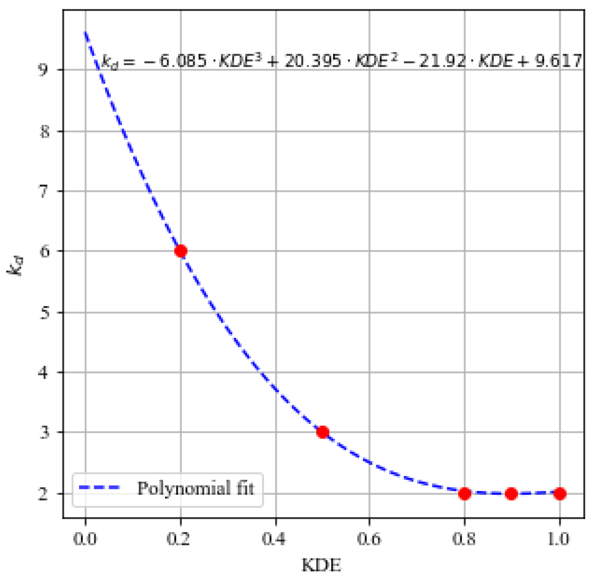
2.7. Density Factor and Adaptive Warning Threshold

Once the feature importance and the KDE are computed, each load combination has a density value, which can be used to adapt the warning threshold. This was achieved by transforming the k factor in Equation (3) into an adaptive value (k_d) by means of a polynomial fit, defined from the following couples (

Table 2. Values of k_d factor associated with density values for defining polynomial fit.

Density Value	kd
0.2	6
0.5	3
0.8	2
0.9	2
1.0	2

).

With this choice, we assign a warning threshold of 2σ_ϵ for areas of density over 0.8, which would cover 95% of the data in cases of normal distribution. As the KDE decreases, k_d increases, as does the width of the warning threshold. The polynomial is shown in Figure 4.

Once the k_d factor is calculated for each sample, it is applied to compute the warning threshold by multiplying the standard deviation (Equation (11)). Each sample is assigned its warning threshold, which is widened in low-density areas, while maintaining a threshold of 2σ_ϵ for samples with high KDE.

$$W{T}_{KDE}=\widehat{y_i}\pm k_d\times {\mathsf{\sigma }}_{\mathsf{ϵ}}$$

(11)

3. Results

3.1. BRT Model and Feature Importance

As mentioned in Section 2.2, a BRT model was fitted to predict each pendulum’s response in both the training and testing sets, using level, temperature, and their derived variables as inputs. The observed and predicted values from each BRT were used to calculate the residuals.

Table 3. Top feature importance inputs and standard deviation of the residuals by training/test set and output variable.

Pendulum	$\mathit{T}\mathit{o}\mathit{p}\_\mathit{I}\mathit{m}{\mathit{p}}_{\mathit{L}}$$/\mathit{T}\mathit{o}\mathit{p}\_\mathit{I}\mathit{m}{\mathit{p}}_{\mathit{T}}$	$\mathit{I}\mathit{m}{\mathit{p}}_{\mathit{L}}$$/\mathit{I}\mathit{m}{\mathit{p}}_{\mathit{T}}$	σϵ (mm)	σϵ (mm)
	Train1			Test1
P1DR1	Level_001D/Tair_090D	0.25/0.74	0.529	1.753
P1DR4	Level_001D/Tair_090D	0.30/0.68	0.400	1.601
P5DR1	Level_001D/Tair_060D	0.15/0.83	0.579	1.024
P6IR1	Level_001D/Tair_030D	0.12/0.87	0.519	1.058
	Train2			Test2
P1DR1	Level_001D/Tair_090D	0.43/0.56	0.554	1.258
P1DR4	Level_001D/Tair_120D	0.60/0.38	0.415	1.111
P5DR1	Level_001D/Tair_060D	0.23/0.75	0.602	0.950
P6IR1	Level_001D/Tair_030D	0.18/0.81	0.572	0.936

presents the importance of $Top\_Im{p}_L$ and $Top\_Im{p}_T$, along with the most significant features within each group by test set and the standard deviation of the residuals. It was noted that $Top\_Im{p}_L$ remains consistent (Level_001D) across all outputs and both training sets. This suggests that the effect of hydrostatic load is immediate—reflected by the lower relevance of moving average variables—as expected for this type of dam. It also demonstrates that the BRT model was able to correctly capture this pattern without requiring explicit variable selection.

Additionally, the standard deviation of the residuals for the training set (σ_ϵ) was calculated, showing no significant variation between training sets. There is, however, a great decrease in accuracy for all models in the test set. Although these models are known to overfit the training data to some extent (which does not prevent them from being competitive in terms of accuracy), such an effect is notably amplified in this case due to the evolution of the input loads. In particular, the hydrostatic load for many test set samples is lower than the minimum recorded in the training set. This can also be verified by observing that the increase in error between training and test sets is not so pronounced in Train/Test₂, where the difference in reservoir level between the training and test sets is smaller.

As for the effect of air temperature, the moving averages are more influential than the daily records. Again, this reflects the thermal inertia of concrete arch dams and confirms that the model correctly captured such well-known behavior in spite of being fed highly correlated features. The period for the most relevant moving average changes from 90 and 120 days for the displacements in the higher cantilever to 60 and 30 days for the deformations closer to the abutments.

In addition, the relative influence of the loads significantly changes between Train₁ and Train₂ for all outputs. In particular, for the extended training set, reservoir level is more relevant (and vice versa for the temperature). This is due to the specific evolution of the reservoir level: it remained mostly high in Train₁, resulting in a higher influence of temperature (in the extreme hypothetical situation in which the hydrostatic pressure would be fixed, it would have no influence). With a wider range of variation for the reservoir level, its importance increases in Train₂.

3.2. KDE Area

Figure 5 and Figure 6 present the KDE area calculated for all outputs in Train₁ and Train₂, respectively. The effect of the adaptive bandwidths (based on $Im{p}_L$ and $Im{p}_T$ using Equations (9) and (10)) can be observed in the shape of the contour curves of density. When the difference between $Im{p}_L$ and $Im{p}_T$ is high (e.g., P6IR1, Train₁), the density function is bumpier, with higher gradients in the direction of the more important input (the y-axis in our case). As such differences decrease, the density function becomes smoother, as seen in P1DR1, Train₂. The same applies to the other pendulums, although it is not as obvious due to the smaller difference in importance. In these plots, the white circles represent the samples from the testing set, and their size is proportional to the residual value. This shows that the model accuracy tends to be lower in areas with low KDE density, which confirms the initial assumption on the lower reliability of BRT model predictions when extrapolating.

In these plots, the negative values of the normalized loads correspond to situations in which the model is extrapolating, i.e., the load values are out of the range of variation in the training set. The in-range area is denoted by dashed lines, and it is useful to note that prediction error is also high in low-density areas, even if the model is not strictly extrapolating.

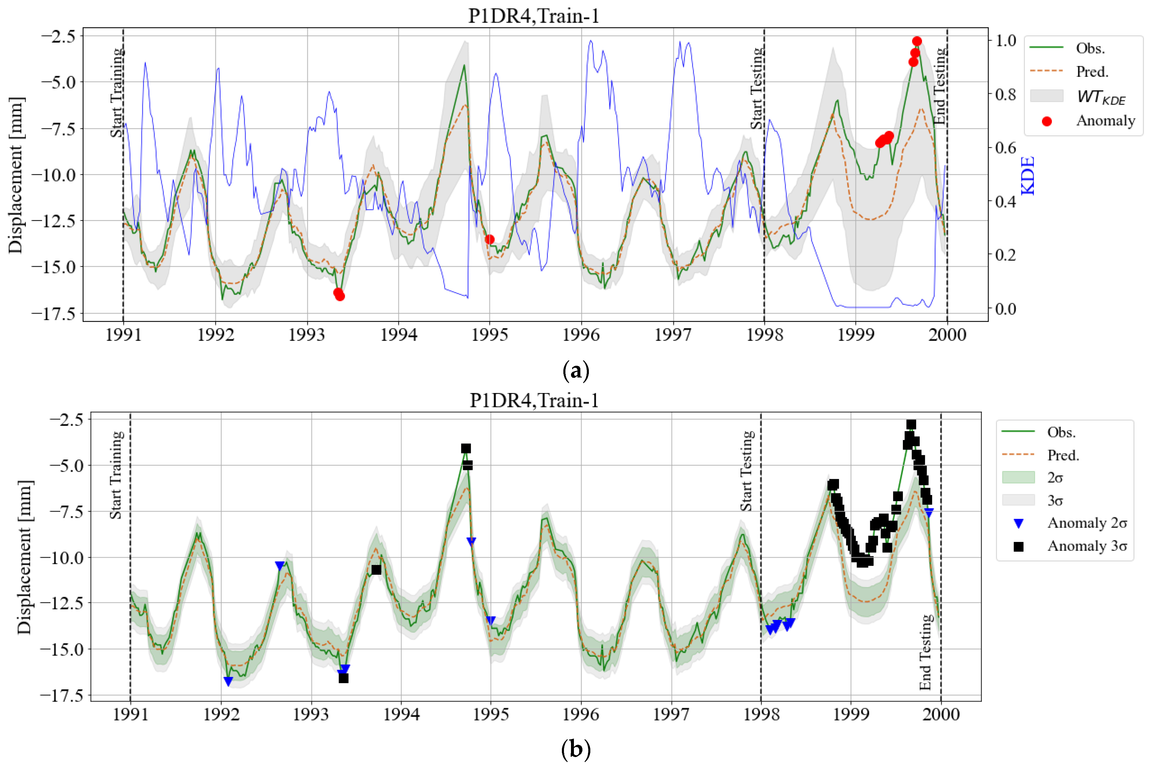
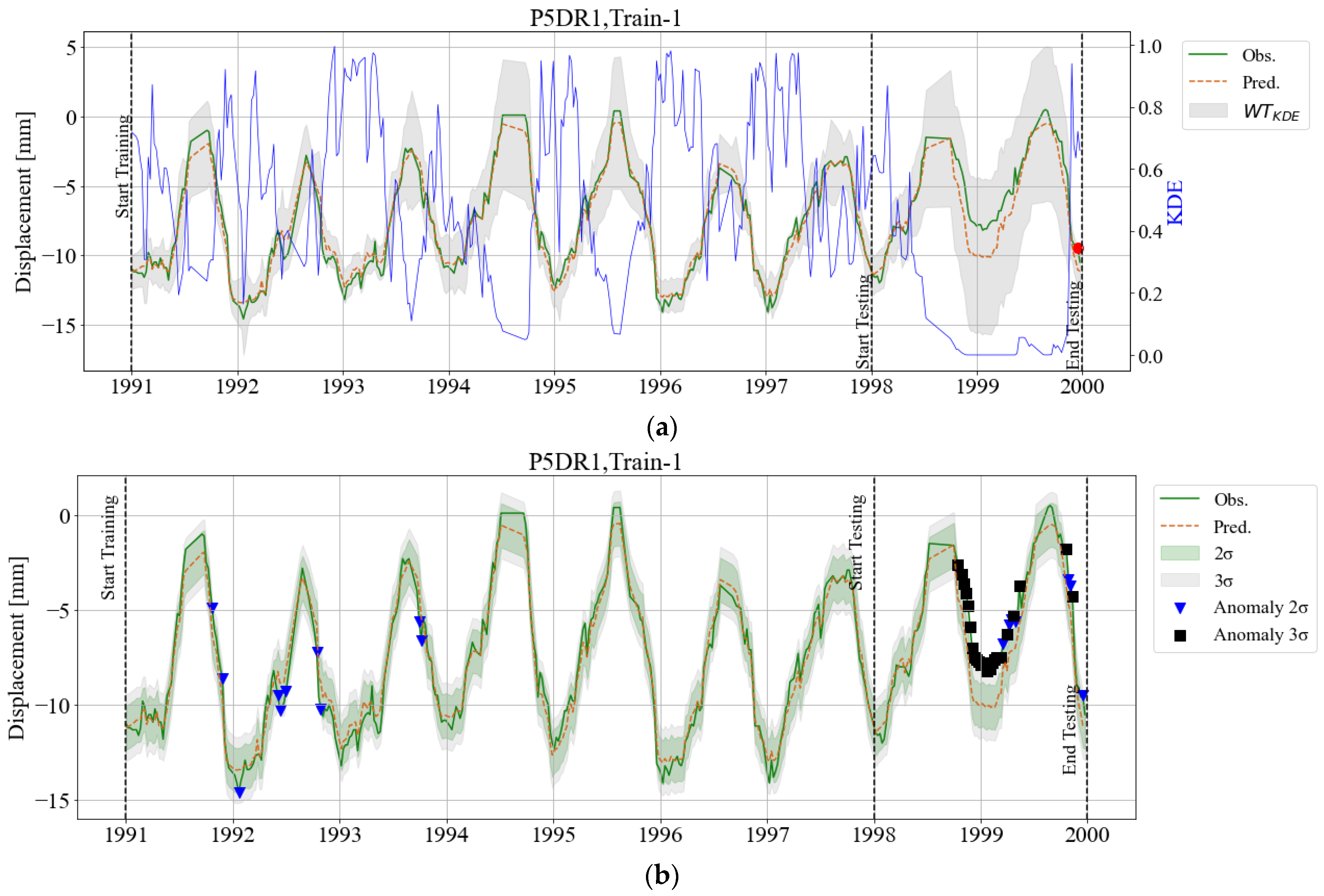
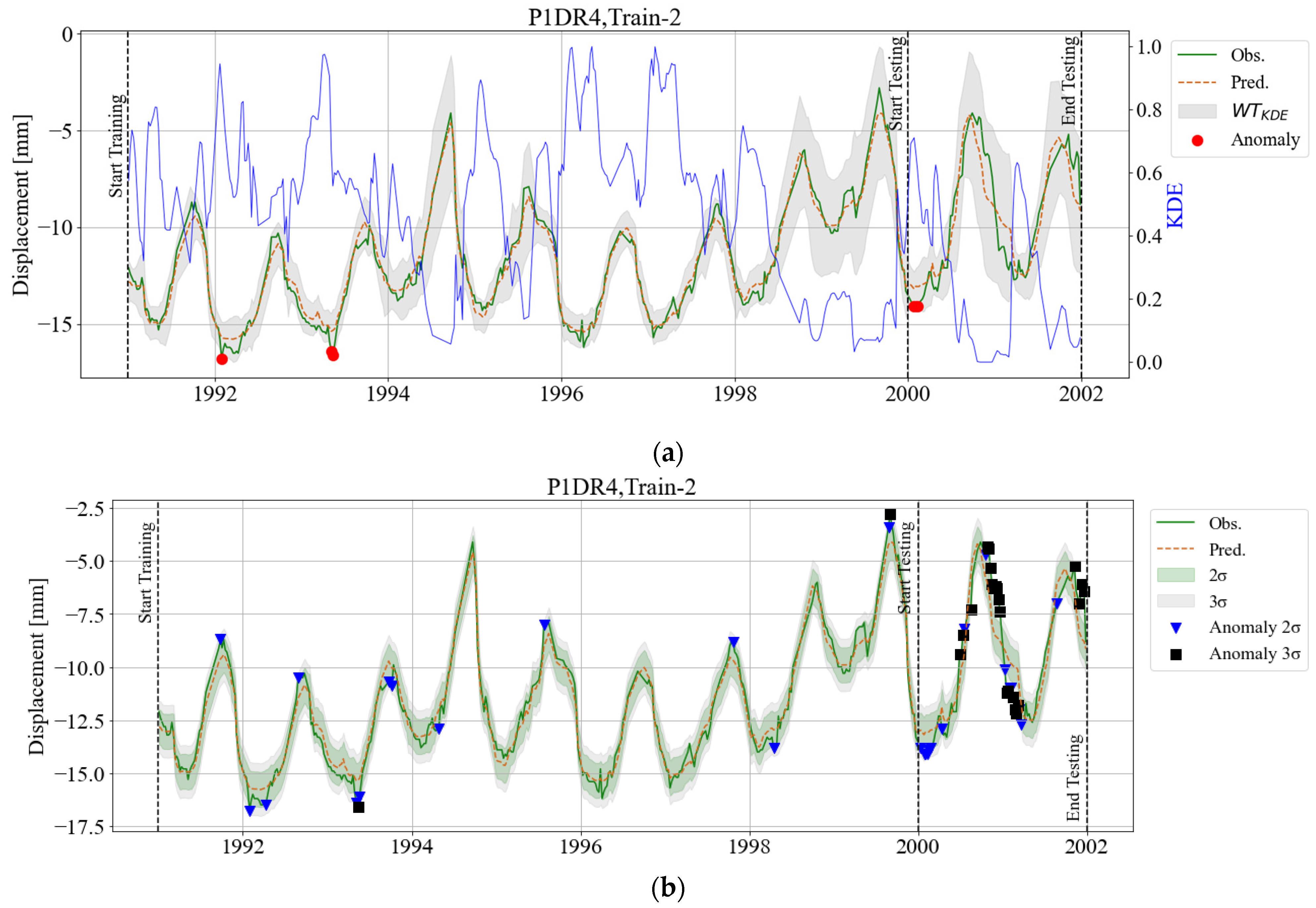
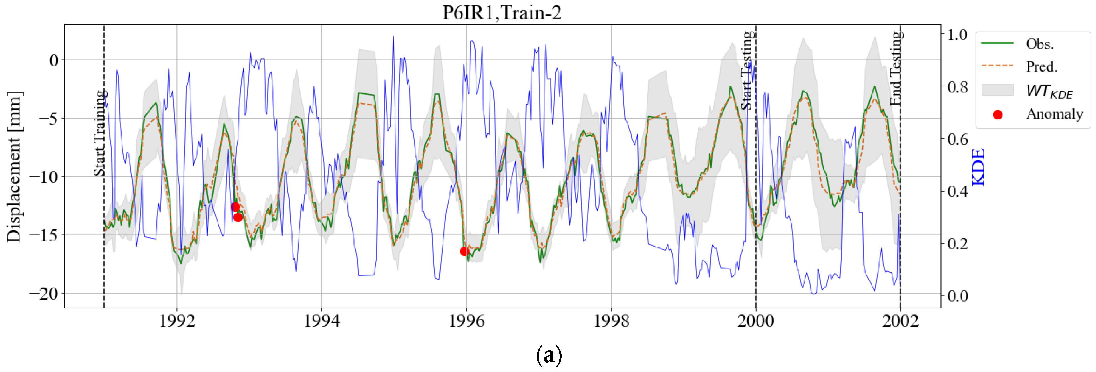
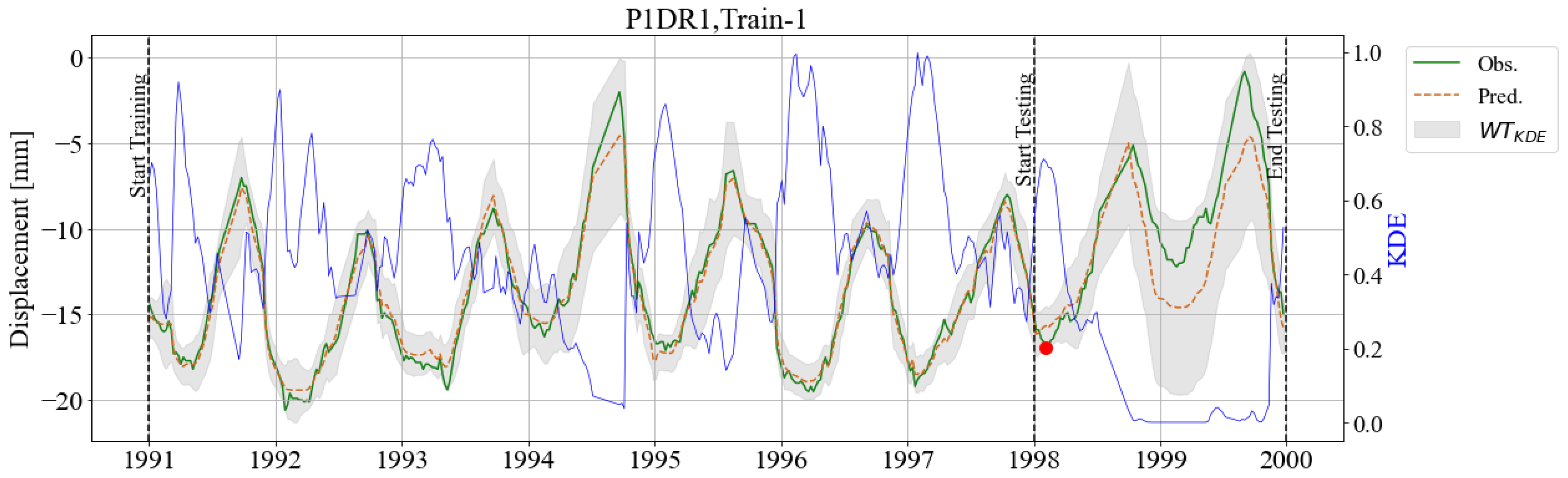
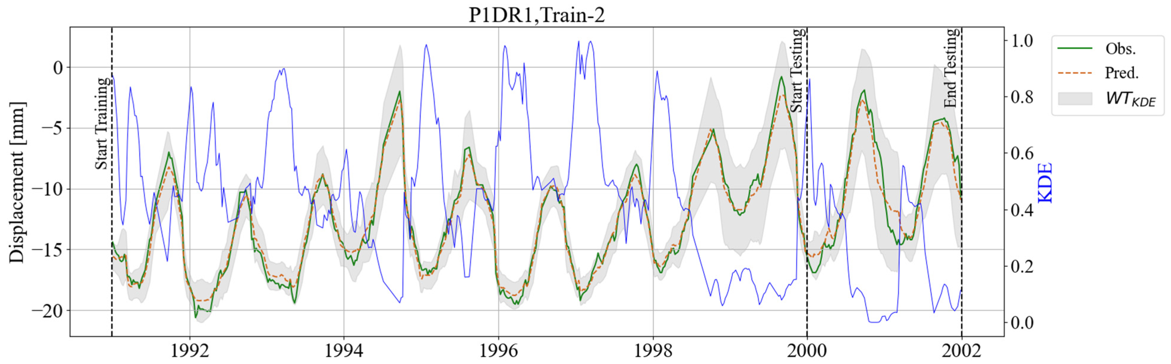
3.3. Adaptive Warning Threshold (WT_KDE)

The main result of the methodology is the characterization of the dam displacement in the test sets. The KDE values computed for each sample in the test set were extracted from the data shown in Figure 5 and Figure 6 and used to compute the adaptive warning threshold by applying Equation (11). The results for P1DR1-Train₁ are presented in Figure 7. In addition to the warning threshold, the plot shows the KDE value on the right vertical axis. The inverse relation between KDE and the width of the WT can thus be noticed. In particular, the low reservoir level after mid-1998 results in a density value close to zero and a very wide interval. As a result, the observed response is considered healthy, in spite of being higher than the BRT predictions. In this case, there is one record out of the WT_KDE that is incorrectly classified as anomalous, though the distance to the lower limit of the healthy area is very small (0.09 mm).

Although the method is intended for online dam safety control, e.g., not for verification of historical data, the benefits of the dynamic threshold can also be verified in the records from summer 1994, where the reservoir level was also low. The density value is small, and the warning threshold widens, which avoids misclassification of these values as anomalous, despite the higher residual. This behavior also shows that overfitting is under control for the BRT model.

The performance of the baseline approach, with fixed thresholds set at two and three times the standard deviation of the residuals, is shown in Figure 8. The number of misclassified records is much higher in both cases. The main difference can be observed in the test set, in the period of low reservoir level. The higher error of the BRT model, together with the constant width of the threshold, results in a high number of false anomalies that are persistent over time. This occurs for both 2σ_ϵ and 3σ_ϵ and exemplifies the improvement of the proposed approach, in which the width of the interval is adapted to consider the density of the load combination.

For the training set, the 2σ_ϵ approach finds eight anomalous records, six of which are close to the threshold limit. The remaining two correspond to the response in summer 1994 and are also considered anomalous by the 3σ_ϵ approach, in contrast to the dynamic threshold. This is an additional verification of the benefits of the proposed approach.

As for the extended training set, the results are similar for P1DR1 (Figure 9). In this case, the density values in the test set are slightly higher, but the adaptive threshold is also widened, according to the KDE value, which results in all records being correctly classified as healthy. The higher variety of the training data also has an effect on model accuracy: predictions follow the observations in Test₂ much more closely than in Test₁, which also contributes to the correct identification as normal behavior.

Such improved accuracy of the BRT model is also highly influential in the results of the conventional approach, as shown in Figure 10. The number of misclassifications decreases in the test set, as well as the distance to the threshold. However, even for a more accurate model and the 3σ_ϵ option (the more conservative approach), the number of false positives in the test set is 15. This is because the increased accuracy results in narrow intervals, which counteract the positive effect of lower error. Interestingly, the records in August 1994, which were incorrectly classified when Train₁ was used, are now inside the interval due to the increased prediction accuracy.

The results for the remaining three pendulums, both for the proposed and the baseline approaches, are similar to those presented and discussed for P1DR1 and are summarized in

Table 4. Percentage of detected anomalies using 2σ_ϵ, 3σ_ϵ, and WT_KDE as warning thresholds.

	$\mathit{T}\mathit{r}\mathit{a}\mathit{i}{\mathit{n}}_1$ (294 Samples)			$\mathit{T}\mathit{e}\mathit{s}{\mathit{t}}_1$ (81 Samples)
Pendulum	2σϵ (%)	3σϵ (%)	WTKDE (%)	2σϵ (%)	3σϵ (%)	WTKDE (%)
P1DR1	2.7	0.7	0.0	64.2	59.3	1.2
P1DR4	3.7	1.4	0.7	66.7	59.3	11.1
P5DR1	3.7	0.0	0.0	43.2	33.3	1.2
P6IR1	4.1	0.0	0.7	42.0	30.9	1.2
	$\mathit{T}\mathit{r}\mathit{a}\mathit{i}{\mathit{n}}_{\mathbf{2}}$ (375 Samples)			$\mathit{T}\mathit{e}\mathit{s}{\mathit{t}}_{\mathbf{2}}$ (82 Samples)
P1DR1	4.8	0.0	0.5	39.0	18.3	0.0
P1DR4	4.0	0.5	0.8	43.9	26.8	1.2
P5DR1	4.3	0.3	0.3	25.6	11.0	0.0
P6IR1	4.0	0.8	0.8	24.4	6.1	0.0

, which includes the percentage of false anomalies identified for both approaches and training sets and all response variables. For the training datasets, the percentage of anomalies detected with fixed thresholds is in the range of the theoretical target for the case of normal distribution (4.56% for 2σ_ϵ and 0.28% for 3σ_ϵ), while WT_KDE resulted in lower values in general, always closer to the 3σ_ϵ results. The main difference is observed for the test sets, which is the main goal of the method (online anomaly detection, based on a predictive model trained on historical data). In seven out of the eight scenarios considered, one or zero false anomalies are reported. For P1DR4-Test₁, the method was less efficient, identifying 11.1% of the observations as anomalies.

Figure 11 shows the results for P1DR4 and the Train/Test₁ set. The nine false anomalies are grouped into two periods, all in 1999 and close to the upper limit of the threshold (between 0.03 and 0.48 mm). Although this performance is still better than the conventional approach, the percentage of false anomalies is above the desired threshold (1–5%). This result is due to the excessive increase in model error between training and test. As seen in Table 3, the standard deviation of the residuals increases by a factor of four, from 0.40 in Train₁ to 1.60 in Test₁. This ratio is much greater than in any other scenario. The closest value is 3.3 for P1DR1-Train₁. We can observe that during the same two periods in which false positives were detected for P1DR4, the observations in P1DR1 were close to (though still below) the upper limit of the dynamic warning threshold (Figure 7).

To verify this potential explanation, and for further assessment of the methodology, we repeated the process for P1DR4 for a training set ending on 31 December 1998 (Figure 12). This can be considered a more realistic approach to professional practice, with models and warning threshold definitions being updated every year. The results show that false positives are avoided, mainly because of a reduction in prediction error.

The plots for other outputs are included in Appendix A.

4. Discussion and Final Remarks

The example was specifically chosen to illustrate the benefits of the method: the range of variation of the reservoir level is clearly and consistently out of the limits in the training set, which implies that the accuracy of model predictions is much lower. This resulted in a clear difference with respect to the conventional approach, based on a fixed threshold associated with the errors in the training set. Of course, such a difference would be less apparent in other settings, but the assumptions were verified, and thus the method was proven to improve the fixed threshold approach. Its application would thus result in more precise and efficient anomaly detection.

The work was oriented to define warning thresholds to be applied online to newly generated response data, with the final aim of early anomaly detection. However, it also proved to be useful when verifying historical data. The results of the conventional approach were in agreement with its theoretical fundamentals, yielding a percentage of anomalies close to 5% for 2σ_ϵ and 1% for 3σ_ϵ. The adaptive warning thresholds had similar performance to the 3σ_ϵ approach, with less than 1% of records out of the interval, which in this context are considered false anomalies. This result has merit, since for high-density areas (with KDE higher than 0.8), the adaptive threshold is computed with k_d = 2, thus resembling the 2σ_ϵ option. This is not relevant for the case study presented, which corresponds to healthy data: the perfect performance would result in zero anomalous values. However, in a real practical context, in case an anomaly occurs, a narrower interval is more efficient, since it allows for earlier detection of anomalies. In this regard, the proposed approach resembles the 2σ_ϵ rule for high-density regions and only widens to account for the increase in prediction error for load values with low representation in the training set.

The methodology was developed with the aim of being applicable to other output variables and dam typologies. Some features may seem tailored to the case of displacements in arch dams, such as the consideration of the thermal inertia through the moving averages of air temperatures, or the calculation of the relative influence of hydrostatic and thermal loads. However, the same process is valid, for instance, to consider seepage flow in an embankment dam, except that some steps could be omitted. As mentioned before, the same set of inputs can be used with BRTs, even if some are negligible for certain outputs: the algorithm mostly selects the influential features and discards the others. Also, the effect of air temperature, if negligible, could be omitted for the KDE calculation, which would thus be computed mostly as a function of reservoir level variation. In spite of that, the overall process is still useful.

The relation between the KDE value and the k_d factor applied to σ_ϵ for computing the width of the warning threshold was defined to ensure that k_d equals 2 for high-density areas and progressively increases as the KDE decreases. We acknowledge that such a method is not optimal, but it is shown to be effective in practice. An alternative polynomial would yield similar results, provided that a similar trend is followed.

The definition of the KDE function accounts for the relative influence of each of the main loads. A simpler approach might be beneficial while keeping the benefits of differentiating between loads. In particular, the decrease in KDE between high-density areas is essential for effective adaptation of the warning threshold.

One limitation of the proposed methodology is that it relies on feature importance derived from the BRT model. If a different predictive method is employed, some alternative techniques could be needed to select the appropriate axes for KDE calculation. However, as mentioned before, similar results would probably be obtained with a less detailed calculation of load influence. For instance, a conventional sensitivity analysis would probably be useful.

Overall, the proposed KDE-based adaptive threshold offers a refined anomaly detection framework that supports dam safety monitoring in fluctuating conditions, minimizing false alarms and improving model robustness across varying load scenarios. This approach enables dam safety professionals to monitor critical infrastructure with a higher degree of confidence in the predictive model’s output, ensuring a safer, more reliable response to potential structural anomalies.

In summary, the goals defined at the outset of this work—namely, to improve conventional fixed-threshold approaches through a KDE-based adaptive method for anomaly detection—were satisfactorily achieved, as demonstrated by the enhanced performance and interpretability in the presented case study.

References

1. Perera, D.; Smakhtin, V.; Williams, S.; North, T.; Curry, R. Ageing Water Storage Infrastructure: An Emerging Global Risk; UNU-INWEH Report Series; Issue 11; United Nations University Institute for Water, Environment and Health: Hamilton, ON, Canada, 2021. [Google Scholar] [CrossRef]
2. ICOLD Incident Database Bulletin 99 Update: Statistical Analysis of Dam Failures; International Commission on Large Dams (ICOLD): Paris, France, 2019.
3. Swiss Committee on Dams. Methods of analysis for the prediction and the verification of dam behaviour. In Proceedings of the 21st Congress of the International Comission on Large Dams, Montreal, QC, Canada, 16–20 June 2003. [Google Scholar]
4. Cheng, L.; Zheng, D.L. Two online dam safety monitoring models based on the process of extracting environmental effect. Adv. Eng. Softw. 2013, 57, 48–56. [Google Scholar] [CrossRef]
5. Li, B.; Yang, J.; Hu, D.J. Dam monitoring data analysis methods: A literature review. Struct. Control Health Monit. 2019, 27, e2501. [Google Scholar] [CrossRef]
6. Pereira, S.; Magalhães, F.; Gomes, J.P.; Cunha, Á.; Lemos, J.V. Dynamic monitoring of a concrete arch dam during the first filling of the reservoir. Eng. Struct. 2018, 174, 548–560. [Google Scholar] [CrossRef]
7. Yi, T.-H.; Li, H.-N.; Gu, M. Optimal sensor placement for structural health monitoring based on multiple optimization strategies. Struct. Des. Tall Spéc. Build. 2011, 20, 881–900. [Google Scholar] [CrossRef]
8. Yi, T.-H.; Li, H.-N.; Zhang, X.-D. Sensor placement on Canton Tower for health monitoring using asynchronous-climb monkey algorithm. Smart Mater. Struct. 2012, 21, 125023. [Google Scholar] [CrossRef]
9. Salazar, F.; Morán, R.; Toledo, M. Data-Based Models for the Prediction of Dam Behaviour: A Review and Some Methodological Considerations. Arch Comput. Methods 2017, 24, 1–21. [Google Scholar] [CrossRef]
10. Salazar, F. A Machine Learning Based Methodology for Anomaly Detection in Dam Behaviour. Ph.D. Thesis, Universitat Politècnica de Catalunya, Les Corts, Barcelona, 2017. [Google Scholar]
11. Willm, G.; Beaujoint, N. Les méthodes de surveillance des barrages au service de la production hydraulique d’Electricité de France-Problèmes ancients et solutions nouvelles. In Proceedings of the 9th ICOLD Congres, Istanbul, Türkiye, 4–8 September 1967; pp. 529–550. [Google Scholar]
12. Salazar, F.; Conde, A.; Irazábal, J.; Vicente, D.J. Anomaly Detection in Dam Behaviour with Machine Learning Classification Models. Water 2021, 13, 2387. [Google Scholar] [CrossRef]
13. Su, H.; Chen, Z.; Wen, Z. Performance improvement method of support vector machine-based model monitoring dam safety. Struct. Control Health Monit. 2015, 23, 252–266. [Google Scholar] [CrossRef]
14. Mata, J.; Salazar, F.; Barateiro, J.; Antunes, A. Validation of Machine Learning Models for Structural Dam Behaviour Interpretation and Prediction. Water 2021, 13, 2717. [Google Scholar] [CrossRef]
15. Hellgren, R.; Malm, R.; Ansell, A. Performance of data-based models for early detection of damage in concrete dams. Struct. Infrastruct. Eng. 2021, 17, 275–289. [Google Scholar] [CrossRef]
16. Lin, C.; Chen, S.; Hariri-Ardebili, M.A.; Li, T.; Del Grosso, A. An Explainable Probabilistic Model for Health Monitoring of Concrete Dam via Optimized Sparse Bayesian Learning and Sensitivity Analysis. Struct. Control Health Monit. 2023, 2023, 2979822. [Google Scholar] [CrossRef]
17. Li, X.; Li, Y.; Lu, X.; Wang, Y.; Zhang, H.; Zhang, P. An online anomaly recognition and early warning model for dam safety monitoring data. Struct. Health Monit. 2020, 19, 796–809. [Google Scholar] [CrossRef]
18. Su, H.; Yan, X.; Liu, H.; Wen, Z. Integrated Multi-Level Control Value and Variation Trend Early-Warning Approach for Deformation Safety of Arch Dam. Water Resour. Manag. 2017, 31, 2025–2045. [Google Scholar] [CrossRef]
19. Mata, J.; Tavares de Castro, A.; Sá da Costa, J.M.; Barateiro, J.; Miranda, P. Threshold Definition for Internal Early Warning Systems for Structural Safety Control of Dams. Application to a Large Concrete Dam, October 2012. In Proceedings of the First International Dam World Conference 2012, Maceió, Brazil, 8–11 October 2012. [Google Scholar]
20. Mata, J.; Miranda, F.; Antunes, A.; Romão, X.; Santos, J. Characterization of Relative Movements between Blocks Observed in a Concrete Dam and Definition of Thresholds for Novelty Identification Based on Machine Learning Models. Water 2023, 15, 297. [Google Scholar] [CrossRef]
21. Klun, M.; Salazar, F.; Simon, A.; Malm, R.; Hellgren, R. Behaviour Prediction of a Concrete Arch Dam: Description and Synthesis of Theme A. In Proceedings of the 16th International Benchmark Workshop on Numerical Analysis of Dams, Ljubljana, Slovenia, 5–6 April 2022. [Google Scholar]
22. Salazar, F.; Toledo, M.A.; Oñate, E.; Morán, R. An empirical comparison of machine learning techniques for dam behaviour modelling. Struct. Saf. 2015, 56, 9–17. [Google Scholar] [CrossRef]
23. Salazar, F.; Irazábal, J.; Conde, A. SOLDIER: SOLution for Dam behavior Interpretation and safety Evaluation with boosted Regression trees. SoftwareX 2024, 25, 101598. [Google Scholar] [CrossRef]
24. Elith, J.; Leathwick, J.R.; Hastie, T. A working guide to boosted regression trees. J. Anim. Ecol. 2008, 77, 802–813. [Google Scholar] [CrossRef] [PubMed]
25. Müller, A.C.; Guido, S. Introduction to Machine Learning with Python: A guide for data scientists. O’Reilly Media: Sebastopol, CA, USA, 2017. [Google Scholar]
26. Parzen, E. On Estimation of a Probability Density Function and Mode. Ann. Math. Stat. 1962, 33, 1065–1076. [Google Scholar] [CrossRef]
27. Chen, Y.-C. A tutorial on kernel density estimation and recent advances. Biostat. Epidemiol. 2017, 1, 161–187. [Google Scholar] [CrossRef]
28. Xiong, L.; Liang, J.; Qian, J. Multivariate Statistical Process Monitoring of an Industrial Polypropylene Catalyzer Reactor with Component Analysis and Kernel Density Estimation. Chin. J. Chem. Eng. 2007, 15, 524–532. [Google Scholar] [CrossRef]
29. Silva-Cancino, N.; Salazar, F.; Irazábal, J.; Mata, J. Adaptive warning thresholds in dam safety using kernel density estimation. In Proceedings of the Fifth International Dam World Conference, Lisbon, Portugal, 13–17 April 2025. [Google Scholar]
Figure 1. Flowchart of methodology.
Infrastructures 10 00158 g001
Figure 2. Dam geometry and location of the pendulums considered for the analysis.
Infrastructures 10 00158 g002
Figure 3. Reservoir water level and air temperature time series, divided into training and testing sets.
Infrastructures 10 00158 g003
Figure 4. Adaptive kd as a function of the KDE. The red dots are the threshold-defining points, and the blue curve shows the polynomial fit.
Infrastructures 10 00158 g004
Figure 5. KDE area for each output in Train1: P1DR1 (a), P1DR4 (b), P5DR1 (c) and P6IR1 (d). White circles are the test set samples, and their size is proportional to the residual. The dashed rectangles highlight the range of variation of the variables in the training set.
Infrastructures 10 00158 g005
Figure 6. KDE area for each output in Train2: P1DR1 (a), P1DR4 (b), P5DR1 (c) and P6IR1 (d). White circles are the test set samples, and their size is related to the residual. The dashed rectangles highlight the range of variation of the variables in the training set. The limits are equal to those in Train1 because the normalization is updated for the extended training set.
Infrastructures 10 00158 g006
Figure 7. P1DR1: Observed and predicted data, adaptive warning threshold, and KDE (blue line) for each sample in Train1 and Test1.
Infrastructures 10 00158 g007
Figure 8. P1DR1: Observed and predicted data and warning threshold for each sample in Train1 and Test1. Conventional approach based on 2–3 times the standard deviation of the residuals. Note that by definition, all anomalies found with the 3σϵ are also out of the interval if 2σϵ is applied.
Infrastructures 10 00158 g008
Figure 9. P1DR1: Observed and predicted data, adaptive warning threshold, and KDE (blue line) for each sample in Train2 and Test2.
Infrastructures 10 00158 g009
Figure 10. P1DR1: Observed and predicted data and warning threshold for each sample in Train2 and Test2. Conventional approach based on 2–3 times the standard deviation of the residuals.
Infrastructures 10 00158 g010
Figure 11. P1DR4: Observed and predicted data, adaptive warning threshold, and KDE (blue line) for each sample in Train1 and Test1.
Infrastructures 10 00158 g011
Figure 12. P1DR4: Observed and predicted data, adaptive warning threshold, and KDE (blue line) for each sample for a training set ending on 31 December 1998.
Infrastructures 10 00158 g012