A Probabilistic Design Framework for Semi-Submerged Curtain Wall Breakwaters

Abstract

Semi-submerged curtain breakwaters are increasingly favored to protect marinas and other microtidal basins, yet they are still almost exclusively designed with deterministic wave transmission equations. This study introduces a fully probabilistic design framework that translates uncertainty in wave climate and water level design parameters into explicit confidence limits for transmitted wave height. Using Latin Hypercube Sampling, input uncertainty is propagated through a modified Wiegel transmission model, yielding empirical distributions of the transmission coefficients K_t and H_t. Our method uses the associated safety factor required to satisfy a 95% non-exceedance criterion, SF₉₅. Regression analysis reveals the existence of a strong inverse linear relationship (R = −0.9) between deterministic K_t and the probabilistic safety factor, indicating that designs trimmed to low nominal transmission (e.g., K_t ≤ 0.35) must be uprated by up to 55% once parameter uncertainty is acknowledged, whereas concepts with greater transmission require far smaller margins. Sobol indices show that uncertainty in H_m0 and T_p each contribute ≈40% of the variance in H_t for a tide signal standard deviation of σ_η = 0.16 m, while tides only become equally important when σ_η > 0.30 m. Model-based uncertainty is negligible, standing at under 8%. The resulting lookup equations allow designers to convert any deterministic K_t target into a site-specific probabilistic limit with a single step, thereby embedding reliability into routine breakwater sizing and reducing the risk of underdesigned marina and port structures.

1. Introduction

As effective coastal protection structures, curtain wall breakwaters, which are vertical or sloped, attenuate waves and protect sheltered basins. This includes but is not limited to marinas and ports [1]. Compared to conventional gravity-type breakwaters, curtain wall breakwaters offer notable benefits, including reduced material use and cost-efficiency, which are particularly advantageous in deeper waters [2]. The partial submergence of the curtain promotes ecological connectivity, sediment movement, and enhanced water circulation, contributing significantly to the environmental sustainability and improved water quality of the sheltered basins in marinas and ports [3,4,5].

Despite these clear benefits, the performance of semi-submerged curtain wall breakwaters is highly sensitive to several uncertain parameters, significantly affecting the overall efficacy of wave attenuation. These uncertainties primarily involve environmental factors such as variability in wave climates—including design wave height, peak wave periods, storm surge levels, tidal oscillations and potential sea level rise due to climate change. The conventional deterministic methods traditionally applied in curtain wall design do not address these uncertainties. Deterministic “mean-value” approaches, which rely on average conditions, often fall short of accurately representing the uncertainty found within marine parameters [6,7], potentially leading to an underestimation of the required curtain submergence.

Semi-submerged curtain wall breakwaters are widely employed in coastal protection, especially in microtidal areas (tidal oscillations below 2 m); however, their effectiveness is subject to considerable uncertainties stemming from environmental conditions, and limitations in the predictive modeling of transmission coefficients under an incident irregular wave field [3]. The literature [8,9] highlights the importance of distinguishing between uncertainties arising from model limitations and those resulting from incomplete knowledge of extreme distributions, climate change effects, or imperfect numerical modeling. Key hydrodynamic factors such as significant wave height (H_m0), peak wave period (T_p), and water level fluctuations due to tidal oscillations and storm surge exhibit varying degrees of uncertainty, depending on the determination method used. Direct measurements typically yield lower uncertainty, with coefficients of variation (CoV—the ratio of standard deviation to mean) ranging from 0.05 to 0.10 [8,9], while hindcast and numerical modeling approaches introduce greater variability, with CoVs between 0.10 and 0.20 [8,9,10]. Manual calculations and visual observations present even higher uncertainties. The former reach CoVs between 0.15 to 0.35 and the latter display values of approximately 0.20, respectively [8,9,10]. Additionally, the interdependence of parameters, particularly between wave height and wave period, necessitates the use of advanced statistical techniques such as copula functions or correlation matrices for precise quantification [11,12]. Historically, research on semi-submerged curtain wall breakwaters has primarily concentrated on a deterministic approach to calculate the transmission of water waves under one or two vertical plates, with early studies, such as Wiegel’s calculation of transmission coefficients [13], neglecting the impact of reflected waves on the flow field. Kriebel et al. [14] later refined these calculations by incorporating the effects of reflected waves, but their method still failed to account for disturbances near the thin plate, resulting in persistent deviations from experimental results [15]. All prediction methods have been primarily derived for regular waves, while in the field, irregular and steep waves are found in areas with wind driven waves. Therefore, the conditions in the field do not match assumptions at play in the equation derivation [3]. Understanding these transmission characteristics is vital for improving wave–structure interaction models and optimizing breakwater performance in real-world conditions.

Regarding uncertainty analysis in coastal engineering, previous research has primarily focused on rubble mound and vertical wall breakwaters [16,17,18]. These studies employed reliability-based design, Monte Carlo sampling, and partial safety factor methods. Reliability-based designs assess structural performance by considering safety factors affecting the load and resistance of armor stability formula [17]. Monte Carlo probability sampling has been extensively used to quantify performance reliability under uncertain wave conditions, evaluating risks related to overtopping [16], structural stability [19,20], and progressive damage [17]. However, comprehensive uncertainty quantification, specifically for semi-submerged curtain wall breakwaters, especially when employing systematic probabilistic modeling to explicitly address variability in environmental parameters, has not been explored in the existing literature. This gap underscores the novelty and importance of the current study.

The primary objective of this research is to develop and present a systematic methodology with which to identify, quantify, and propagate uncertainties associated with key environmental parameters influencing the wave attenuation performance of semi-submerged curtain wall breakwaters. By applying statistical methodologies and probabilistic modeling techniques, this research aims to generate more precise probabilistic design guidelines. Specifically, it seeks to deliver robust probabilistic estimates of safety factors for wave transmission coefficients, enhancing predictive capabilities for engineers and ensuring the greater reliability and optimal attenuation performance of curtain wall breakwaters. Because of uncertainties in the input design parameters for semi-submerged breakwaters, we hypothesized that there would be uncertainty in the response wave energy transmission and transmitted wave height. Therefore, we recommend a design equation that includes safety factors, rather than a mean-value approach.

Key environmental uncertainties considered in this study are the design of significant wave height, peak wave periods, storm surges, and the astronomical tide during a storm event. Model uncertainties are also taken into account by comparing experimental measurements of wave transmission of irregular waves with well-known deterministic analytical equations, such as the Wiegel equation [13] and power-modified equation [14] for regular wave transmission underneath semi-submerged breakwaters.

2. Materials and Methods

2.1. Expressions for Calculating Wave Transmission Under Curtain Breakwaters

For the calculation of wave transmission past semi-submerged curtain wall breakwaters, the Wiegel [13] and power-modified [14] equations are well known. The theory behind Wiegel equation [13] is relevant as it is based on the depth-integrated power transmission concept and has been widely applied to estimate wave transmission coefficients in breakwater design. The Wiegel formula [13] assumes a rigid, fixed vertical barrier, making it applicable to semi-submerged curtain wall breakwaters under linear wave conditions (Figure 1). Kriebel et al. [14] modified the Wiegel formula [13], which incorporates wave reflection effects to enhance the accuracy of the wave transmission prediction. The transmission coefficient (K_t) in the Wiegel power transmission theory is derived from the principle that the net wave power transmitted below the structure is a fraction of the total incident wave power, and the transmission coefficient is obtained as follows:

$$K_{t,Wiegel}=\sqrt{{\displaystyle \frac{2k(D-W)-\sinh (2k(D-W))}{\sinh (2kD)+2kD}}}$$

(1)

where k is the wave number, and D is the water depth. A modification by Kriebel et al. introduces wave reflection effects by redefining the transmission coefficient as follows:

$$K_{t,Mod.Power}={\displaystyle \frac{2K_{t,Wiegel}}{1+K_{t,Wiegel}}}$$

(2)

This provides a more accurate estimate for wave transmission, particularly in deeper waters.

Given that Equations (1) and (2) have been established and validated experimentally for regular waves, it is necessary to further validate these equations against irregular wave data, specifically focusing on steep waves that are characteristic of environments with short wind-fetch lengths. In order to perform this procedure, we utilized the results described in the research paper by [3], which tested the wave transmission beneath the semi-submerged curtain breakwater from irregular waves. The modified Wiegel equation [13] has a simple format:

$$K_{t,irregular}=m\cdot K_{t,regular}+c$$

(3)

The accuracy of theoretical models in representing real-world irregular wave transmission is a measure of the uncertainty in the model. Accounting for the model’s uncertainties, m and c parameters in Equation (3) express uncertainty, with confidence bands representing the range of potential errors obtained by fitting Equation (3) to the experimental data of [3]. The results and graphical representations including a mean prediction line along with 5% and 95% exceedance limits, providing a 90% confidence interval for model accuracy, are shown in Section 3.1.

2.2. Uncertainty of Design Parameters

The performance of semi-submerged curtain wall breakwaters is influenced by various environmental, structural, and modeling parameters, each of which exhibits inherent uncertainty due to natural variability, measurement errors, and limitations in predictive models. Quantifying these uncertainties is essential to improving the reliability of breakwater designs and ensuring their effectiveness under extreme conditions.

The uncertainty in environmental parameters primarily arises from wave climate variability. This is evident in the design’s significant wave height (H_m0), peak wave period (T_p), and water level, accounting for storm surge levels and astronomical tide level. The coefficient of variation (CoV) is commonly used to provide information about the uncertainty of an input parameter. The coefficient of variation (CoV) is defined mathematically as the ratio of the standard deviation (σ) to the mean (μ) of a given parameter. This metric provides a standardized measure of dispersion relative to the mean, facilitating comparison across parameters with different units or scales.

Table 1. Coefficient of variation (CoV) for key hydrodynamic parameters based on different methods of determination, highlighting uncertainty ranges from various literature sources.

Parameter	Symbol	Method of Determination	CoV (σ’)	Reference
Sig. wave height	Hm0	Measurement	0.05–0.10	[8,9]
			0.022–0.036	[10]
		Hindcast (SMB method)	0.10–0.20	[8,9]
			0.040–0.049	[10]
		Numerical model	0.10–0.20	[8,9]
			0.040–0.044	[10]
		Manual calculation	0.15–0.35	[8,9]
		Visual observations	0.2	[8,9]
			0.044–0.052	[10]
		-	0.05	[12]
			0.09–0.125	[21]
			0.05	[22] **
			0.1	[11]
			0.1–0.2	[23]
Peak wave period	Tp	Measurement	0.028–0.029	[10]
		Hindcast	0.048–0.055	[10]
		Numerical model	0.043	[10]
		Visual observation	0.036–0.047	[10]
		-	0.05	[12]
			0.2	[21]
			0.12	[11,24]
Mean wave period	Tm	Measurement	0.02	[8,9]
		Visual observations	0.15	[8,9]
		-	0.05	[12]
			0.1–0.2	[23]
Water level (Astronomical tide and surge)	η + ss
			0.15–0.3	[21]
			0.03	[12]
Astronomical tide	η	Sine function approximation of astronomical tide	0.707A * (standard deviation, not CoV)	[11]
		Measurements	Calculated from measurements
Storm surge	ss	Numerical models	0.1–0.25	[8,9]

* A is the amplitude of the sine function approximation of the tidal signal for a particular location. The amplitude of the tidal signal is defined by the average tidal range for a particular location; this value is the standard deviation, defined in meters. ** uncertainty due to distribution fitting for long term return period wave design in the Adriatic Sea.

summarizes the coefficients of variation (CoV, denoted as σ’) for several essential hydrodynamic parameters relevant to coastal engineering, focusing in particular on significant wave height (H_m0), peak wave period (T_p), mean wave period (T_m), and water level variations, including astronomical tides and storm surges. These uncertainties are quantified based on different methods of parameter determination, such as direct measurements, hindcast methods, numerical modeling, manual calculations, and visual observations. Each method presents varying degrees of uncertainty, reflecting the inherent variability in environmental processes, measurement techniques, and model limitations.

The significant wave height (H_m0) demonstrates variability according to the determination method. Direct measurements yield relatively low uncertainties, with the CoVs typically ranging from 0.05 to 0.10 [8,9], while [10] provides an even narrower range from 0.022 to 0.036, highlighting the reliability of direct measurement instruments like wave buoys and pressure sensors. This underscores that when precision is important high, direct measurements offer the most dependable data. In contrast, the SMB hindcast method introduces higher uncertainty, with the CoVs ranging between 0.10 and 0.20 [8,9]. This is due to assumptions and simplifications inherent in hindcast methodologies. Ref. [10] further narrows down this range, providing a CoV of 0.040 to 0.049. Numerical modeling methods present CoVs similar to those of the SMB hindcast approach, typically between 0.10 and 0.20 [8,9] and 0.040 to 0.044 [10]. Nonetheless, these models retain considerable uncertainties due to the calibration of the white-capping term and the availability of wave data for use in the calibration of the term. Manual calculations exhibit significantly higher uncertainty, with coefficients of variation ranging widely from 0.15 to 0.35 [8,9]. This elevated uncertainty stems from human error, subjective judgment, simplified calculations, and the inability to fully capture complex physical processes mathematically. Thus, while manual calculations are accessible and straightforward, their accuracy is limited and thus should be used cautiously, particularly in design contexts. Visual observations, perhaps the simplest and least technologically demanding method, have an estimated CoV of approximately 0.2, according to [8,9], and one ranging from 0.044 to 0.052 according to [10]. Visual methods consistently result in significant uncertainty due to observer biases, difficulty estimating wave heights accurately, and the subjective nature of visual assessments. Other references provide additional CoV values for significant wave height (H_m0) without the specification of a particular method of acquiring the data. For instance, Reference [12] cites a CoV of 0.05 and [21] indicates a range of 0.09 to 0.125. Moreover, Reference [22] reported a notably low CoV of 0.05 for the offshore waves in the Adriatic Sea, but only focused on the uncertainty of the long-term forecasting procedure, such as distribution fitting for high-return-period design waves. Reference [22] did not take into account the uncertainty in the numerical data used for the analysis in itself. In summary, the broad range provided by different studies underscores variability in methodologies, locations, and context-specific factors.

The peak wave period (T_p) similarly exhibits uncertainty, though it is generally lower than that observed for a significant wave height. Measurement-based methods are highly precise, with [10] reporting CoVs of just 0.028 to 0.029. This underscores the reliability of precise instrumentation in determining wave periods, which are crucial for designing coastal and offshore structures. Hindcast methods for peak wave periods display somewhat higher uncertainty, with CoVs between 0.048 and 0.055 [10]. The numerical modeling of peak wave periods shows intermediate uncertainty, with a CoV around 0.043 [10]. The moderate uncertainty reflects the strong predictive capabilities of numerical models when capturing wave periods, even if they are still influenced by model parameterization and assumptions inherent in simulations. Visual observation methods for peak wave period determination produce CoVs between 0.036 and 0.047 [10], indicating lower uncertainty than wave height estimates. However, it is still notable due to inherent subjective observer biases. Reference [11] further broadens this range to include samples with a CoV of 0.12, suggesting variability in observational techniques and conditions, while [21] suggests an even higher CoV of 0.2. The mean wave period (T_m) exhibits a relatively low measurement-based uncertainty of 0.02 [8,9], reflecting high confidence in instrumental wave data capturing average conditions over extended periods. Visual observations for mean wave periods, however, yield significantly higher uncertainty, around 0.15, underscoring the limitations of observer accuracy and subjective interpretations of wave characteristics [8,9]. Reference [23] suggest relatively high values of 0.1–0.2 for CoVs.

Water level variations, encompassing both astronomical tides and storm surges, demonstrate a wide range of uncertainties according to [21]. They suggest that the general CoVs for water levels (astronomical tide and surge combined) range from 0.15 to 0.3. Ref. [12] suggests a less conservative value of 0.03. Ref. [19] set different CoVs of 0.05, 0.12 and 0.2 for West/South/East Korea when considering tidal levels, highlighting the importance of considering the location itself in the quantification of uncertainty. Storm surge modeling individually presents CoVs between 0.1 and 0.25 [8,9], acknowledging the complexities and limitations inherent in predicting storm-driven water level rises. Astronomical tides can be represented separately from storm surges by sine function, with [11] reporting a CoV of 0.707 multiplied by tidal amplitude (A). When measurements of astronomical tides are calculated directly for a specific location, uncertainties for microtidal areas can be lower.

It should be noted that [8,9] focused on uncertainties due to model uncertainties and statistical uncertainties. Uncertainties arising due to a lack of knowledge about the true long-term extreme distribution, the influence of climate changes, or the imperfect physical or numerical modeling are not covered by [8,9].

In many cases, the uncertain parameters influencing wave transmission are not independent, and their interdependencies must be considered when quantifying uncertainty. A particularly strong correlation exists between wave height and wave period, as both parameters are governed by wind-generated storm conditions. This relationship can be captured using correlation matrices or copula functions, which enable the joint representation of statistical dependence. Water depth and draft also exhibit a degree of correlation, as variations in water level due to tides or storm surges can influence the effective submergence of the breakwater.

This study uses the coefficients of variation (CoVs) given in

Table 2. Coefficients of variation (CoV) and standard deviation for key environmental parameters used in this study.

Parameter	Symbol	CoV (σ’)	STD (σ)
Sig. wave height	Hm0	0.10	-
Peak wave period	Tp	0.08	-
Astronomical tide		-	0.707A
Storm surge		0.2	-

for the environmental parameters. The CoVs represent a compromise among many different suggestions and sources from Table 1.

According to [12], in cases where site-specific data is unavailable, all wave parameters are assumed to follow normal distributions, as occurs in this study. Therefore, significant wave height uncertainty is modeled using a normal distribution following the recommendation of the Eurotop manual [12], which states that normal distribution should be used if no site-specific information is available. The mean H_m0 is linked with the mean T_p through the wave steepness parameters of H_m0/L₀ = 0.04 to remain in the region of steep waves. This wave steepens value is typical of low-fetch length [25,26]. The uncertainty in the peak wave period, T_p, itself is also modeled through a normal distribution with the corresponding CoVs from Table 2. The water level uncertainty is modeled through the two components, namely the storm surge and astronomical tide. For simplicity, the effect of storm surge was taken into account by adding 10% of the deepwater significant wave height, H_m0, following the work of [11,27,28]. This assumption corresponds to the wind set-up change owing to extreme wind stress change. Astronomical tide uncertainty is defined using a normal distribution, like other environmental variables, with a CoV that is easily derived during the sine function approximation. In this, the tidal signal is determined to be 0.707 of the sine function amplitude, A.

The uncertainty in model accuracy is also taken into account through the CI of m and c, which are part of Equation (3); these values are reported in Section 3.1.

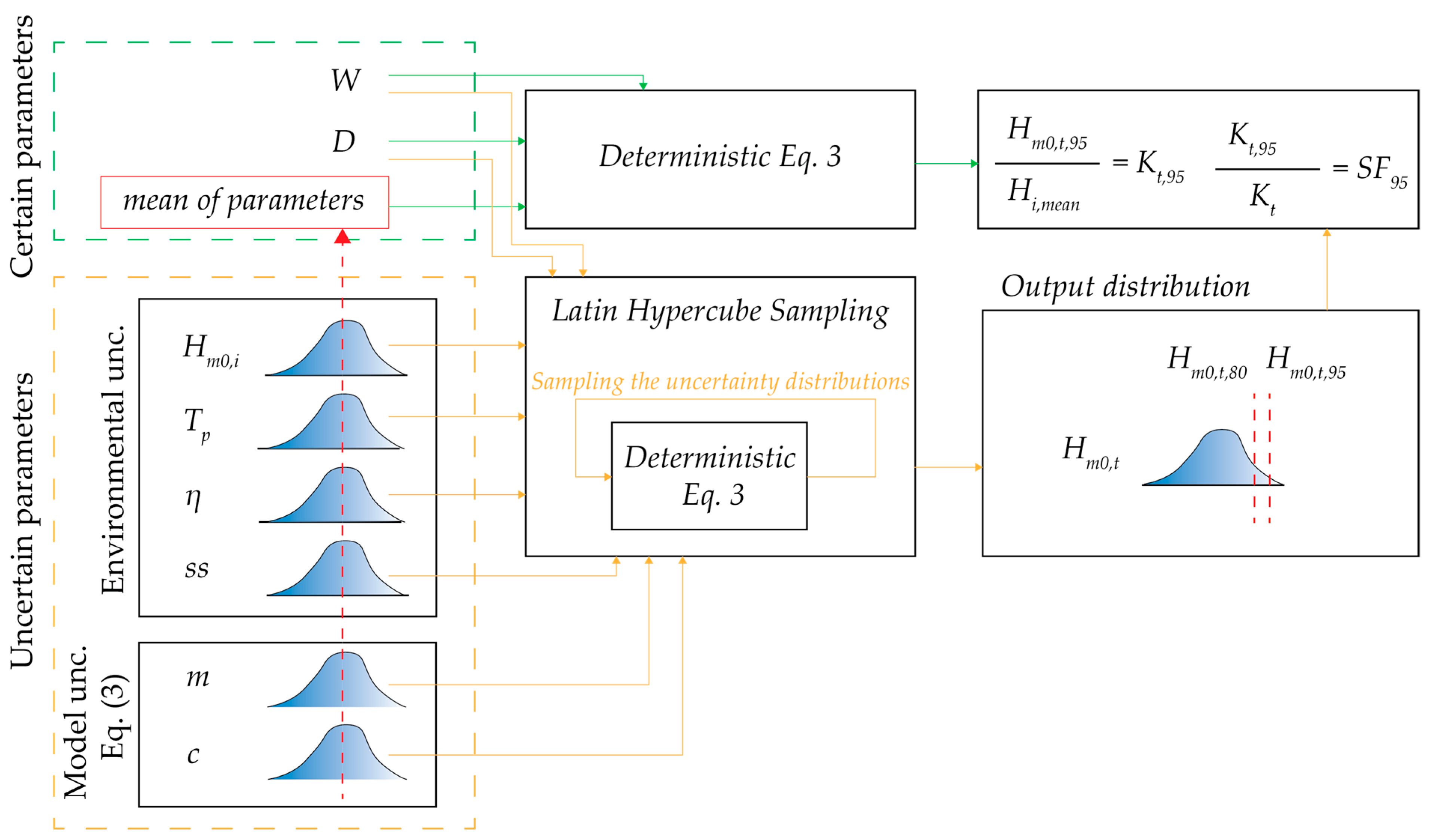
2.3. Uncertainty Quantification Method and Implementation

The quantification of quantification is crucial in assessing the reliability and performance of coastal structures, such as semi-submerged curtain wall breakwaters, by accounting for uncertainty in parameters and their impact on the transmitted significant wave height, H_t. One of the most effective techniques for sampling input parameters from their probability distributions is Latin Hypercube Sampling (LHS). The implementation of LHS improves the efficiency of uncertainty propagation compared to traditional Monte Carlo methods, requiring fewer model evaluations to achieve statistical robustness. Latin Hypercube Sampling, pioneered for nuclear risk problems and now common in coastal engineering, offered a reduction in required realizations relative to simple Monte Carlo when working with the same confidence bounds in our study. That efficiency is reported as being achieved in geotechnical pile analysis by [29] and in flood-risk propagation by [30]. When implementing LHS for uncertainty quantification, the first step involves generating random samples of input parameters, such as significant wave height (H_m0) and peak wave period (T_p) (Figure 2). Uncertainty in these parameters is characterized by the probability distributions discussed in Section 2.2. Each parameter is divided into equal-probability intervals, and samples are drawn systematically to cover the entire range without clustering in any specific region. For the realization of each input parameter, the wave transmission model is run to compute the transmitted significant wave height (H_t), which describes the fraction of wave energy passing through the semi-submerged curtain wall breakwater. The results from each simulation are recorded, and once the model outputs have been collected, a statistical distribution of H_t is estimated. Following the practice of [31,32], a reliability index (β) of 1.65—corresponding to a 95% non-exceedance probability—was selected for the limit state. Another non-exceedance criteria at 80% is selected when the reliability of not exceeding the design transmitted wave heights is not as critical for the operation of the area sheltered by the curtain breakwater. Therefore, the values extracted from the resulting distributions represent the 95th and 80th percentiles of H_t.

As the model in this study is represented with a semi-empirical equation for wave transmission (Equation (3)), the computational model is classified as not being expensive. As such, the specific alternative UQ techniques employed to reduce the number of model evaluations while maintaining accuracy, such as Polynomial Chaos Expansion (PCE) and surrogate modeling (metamodeling)—combined with Gaussian Process (GP) regression or Artificial Neural Networks (ANNs)—are not necessary here. During each test, a total of 1000 calculations are performed to propagate the uncertainty from the input (environmental and model) into the uncertainty of H_t. All tests are given in

Table 3. Coefficients of variation (CoV) for key environmental parameters used in this study; this relates to the uncertainty of the tide level, and is expressed as the standard deviation of the tidal signal from the mean sea level. MSL = 0 m.

N	Hm0,i,mean (m)	Tp,mean (s)	Tide—ση (m)	Surgemean (m)	Sea Depth—D (m)	Draft—W (m)
1	0.7	3.35	0.35	0.07	3	2
2	0.7	3.35	0.35	0.07	5	2
3	0.7	3.35	0.35	0.07	7	2
4	0.7	3.35	0.35	0.07	3	2.5
5	0.7	3.35	0.35	0.07	5	2.5
6	0.7	3.35	0.35	0.07	7	2.5
7	0.7	3.35	0.20	0.07	3	2
8	0.7	3.35	0.20	0.07	5	2
9	0.7	3.35	0.20	0.07	7	2
10	0.7	3.35	0.20	0.07	3	2.5
11	0.7	3.35	0.20	0.07	5	2.5
12	0.7	3.35	0.20	0.07	7	2.5
13	0.7	3.35	0.16	0.07	3	2
14	0.7	3.35	0.16	0.07	5	2
15	0.7	3.35	0.16	0.07	7	2
16	0.7	3.35	0.16	0.07	3	2.5
17	0.7	3.35	0.16	0.07	5	2.5
18	0.7	3.35	0.16	0.07	7	2.5
19	0.5	2.83	0.35	0.05	3	2
20	0.5	2.83	0.35	0.05	5	2
21	0.5	2.83	0.35	0.05	7	2
22	0.5	2.83	0.35	0.05	3	2.5
23	0.5	2.83	0.35	0.05	5	2.5
24	0.5	2.83	0.35	0.05	7	2.5
25	0.5	2.83	0.20	0.05	3	2
26	0.5	2.83	0.20	0.05	5	2
27	0.5	2.83	0.20	0.05	7	2
28	0.5	2.83	0.20	0.05	3	2.5
29	0.5	2.83	0.20	0.05	5	2.5
30	0.5	2.83	0.20	0.05	7	2.5
31	0.5	2.83	0.16	0.05	3	2
32	0.5	2.83	0.16	0.05	5	2
33	0.5	2.83	0.16	0.05	7	2
34	0.5	2.83	0.16	0.05	3	2.5
35	0.5	2.83	0.16	0.05	5	2.5
36	0.5	2.83	0.16	0.05	7	2.5
37	0.9	3.80	0.35	0.09	3	2
38	0.9	3.80	0.35	0.09	5	2
39	0.9	3.80	0.35	0.09	7	2
40	0.9	3.80	0.35	0.09	3	2.5
41	0.9	3.80	0.35	0.09	5	2.5
42	0.9	3.80	0.35	0.09	7	2.5
43	0.9	3.80	0.20	0.09	3	2
44	0.9	3.80	0.20	0.09	5	2
45	0.9	3.80	0.20	0.09	7	2
46	0.9	3.80	0.20	0.09	3	2.5
47	0.9	3.80	0.20	0.09	5	2.5
48	0.9	3.80	0.20	0.09	7	2.5
49	0.9	3.80	0.16	0.09	3	2
50	0.9	3.80	0.16	0.09	5	2
51	0.9	3.80	0.16	0.09	7	2
52	0.9	3.80	0.16	0.09	3	2.5
53	0.9	3.80	0.16	0.09	5	2.5
54	0.9	3.80	0.16	0.09	7	2.5

.

3. Results

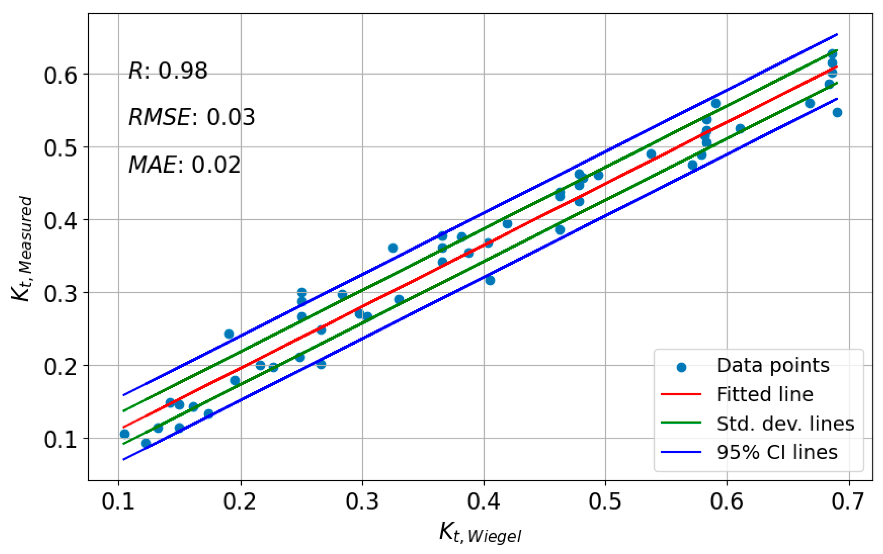
3.1. Applicability of Deterministic Equations for Irregular Waves

Model uncertainty is considered the accuracy with which a model or method can describe a physical process. Therefore, the model uncertainty describes the deviation of the prediction from the measured data due to uncertain model coefficients. This section will present the mean prediction line, accompanied by the 5% exceedance lines that together define the 90% confidence band. The experimental study and the corresponding data analyzed in this section are the same data that were collected and used in the study conducted by [3].

The scatter plot on Figure 3 compares the measured wave transmission coefficients from irregular JONSWAP waves (K_t,Measured) with two theoretical predictions: Wiegel’s power transmission theory (blue dots) [13] and a modified power transmission model (green dots) [14]. The distribution of points around the 1:1 reference line suggests that the Wiegel’s model (blue) aligns more closely with experimental data at lower transmission values (K_t < 0.6), while both the modified power model (blue) and Wiegel’s model (blue) appear to underpredict the transmission by about 15% at higher transmission values (K_t > 0.7). Given that the model and experimental data show some deviations, we adjust the Wiegel equation slightly—as detailed in Section 2.1—in order to produce a modified version that provides a better fit for the irregular wave transmission coefficient data than the original model Wiegel’s model. Given that other environmental uncertainties (shown in Section 3.2) are more significant than model uncertainty in determining H_t, we believe that the simple approximation of Equation (3) is satisfactory for the transmission of irregular waves in this study.

The fitting of Equation (3) by using Wiegel’s equation [13] with irregualar wave data from [3] produces the following best-fit line:

$$K_{t,\mathrm{measured}} = 0.845K_{t,\mathrm{Wiegel}} + 0.027$$

(4)

The slope, estimated at 0.845 with a standard deviation of 0.023, deviates significantly from results indicating unity. A 95% confidence interval indicates a range of 0.80 to 0.89. The ordinate intercept is 0.027 with a standard deviation of 0.0097 and a confidence interval of 0.008–0.046. This shows the weakness of the modified Equation (4), which demonstrates minor transmission, even in cases where no energy transmission is expected with the original Wiegel’s equation [13].

Despite these modest biases, the overall agreement is excellent. The Pearson correlation coefficient is 0.982, indicating that 98% of the variance in the laboratory data is explained by the single predictor provided by Wiegel’s equation [13] (Figure 4). The error magnitudes are relatively small, with a root-mean-square error of 0.029 and a mean absolute error of 0.023. Consequently, Equation (4) captures the underlying behavior of the semi-submerged curtain wall with an irregular incident wave field with high accuracy, and the quantified departures from the ideal 1:1 line can be treated as minor. It should be noted that the fitted line model of Equation (4), which adapts Wiegel’s equation to experimental data, is only applicable within the K_t range of 0.1–0.6, reflecting the typical practical application range for curtain breakwaters.

3.2. Uncertainty Analysis of Wave Energy Transmission

This section delves into the uncertainties associated with various design parameters, aiming to identify the most impactful uncertainties and determine the nature of their influence on transmitted wave height. Figure 5 demonstrates that a higher sea level due to astronomical tide uncertainty at the moment of a storm directly increases the safety factor required to meet the specified exceedance criterion. For the 95th percentile (panel A), the median value of SF₉₅ rises systematically from 1.29 at the smallest astronomical tide level uncertainty (σ_η = 0.16 m) to 1.34 at the intermediate case (σ_η = 0.20 m) and further to 1.39 when the highest tide level uncertainty is considered. Even greater sensitivity is visible in the upper tails of the distributions: the maximum realization increases from 1.52 to 1.50 and reaches 1.66. The same trend appears at the 80th percentile (panel B), albeit with a smaller absolute margin. The median of SF₈₀ shifts from 1.16 through 1.17 to 1.20, while the upper whisker grows from 1.27 to 1.32. Because the target probability of exceedance is lower, the values are naturally lower than in panel A, yet the proportional increase between the scenarios with the lowest and highest tidal uncertainty remains comparable (~5%). Overall, the plots confirm that the increase in the uncertainty in the seal level, defined by the astronomical tide, increases the uncertainty in wave transmission.

Figure 6 reveals a clear threshold behavior controlled by the relative draft (W/L₀). As long as the curtain draft is less than about 14% of the wavelength, the required safety factor increases only marginally. In this “shallow-draft” regime, the median of SF₉₅ creeps from 1.28 at W/L₀ = 0.089 to 1.33 at W/L₀ = 0.143 (panel A), while the median of SF₈₀ moves from 1.16 to 1.17 (panel B).

Once the draft, W, exceeds about 0.15L₀, the situation changes abruptly. At W/L₀ = 0.160, the median SF₉₅ rises to 1.41 and the entire distribution shifts upward; at W/L₀ = 0.160, the median value reaches 1.52 and the upper tail exceeds 1.63. The 80th-percentile factor follows the same trend, with its median increasing from 1.17 to 1.26 and 1.29 at the two largest drafts.

Similar to Figure 6, for water depths up to roughly one-third of the wavelength (D/L₀ ≤ 0.31), the required safety factors only vary slightly. The median of SF₉₅ varies between 1.26 and 1.34, and the SF₈₀ stays close to 1.17.

Beyond that point, however, safety factors increase rapidly. When the depth reaches 40% of the wavelength (D/L₀ = 0.40), the median SF₉₅ jumps to 1.40; at D/L₀ = 0.56, it climbs to 1.49; extreme realizations exceed 1.65. The 80th-percentile factor exhibits the same trend, with its median rising from 1.17 to 1.23 and 1.27 for the deepest settings.

Across the entire tested range of the relative draft W/D parameter, variability is minimal, and the safety factor exhibits no trend with the increase in W/D. Median values of SF₉₅ only vary between 1.29 and 1.34, while the corresponding medians of SF₈₀ remain confined between 1.17 and 1.20. Thus, increasing the draft-to-depth ration does not systematically raise or lower the required design factor, although the spread of the box plots suggests that other parameters significantly influence the safety factors.

Figure 6, Figure 7 and Figure 8 show that uncertainties in environmental and model parameters have the greatest impact at shorter wavelengths, where the relative draft-to-wavelength (W/L) and depth-to-wavelength (D/L) ratios are higher. As with other structures that can transmit incoming wave energy on the lee side, such as floating breakwaters, semi-submerged curtain breakwaters under the impact of wave with higher wavelength correspond with a higher transmission coefficient, K_t. Therefore, it is assumed that a higher K_t will correspond to a lower safety factor. This is considered in Section 3.3.

3.3. Safety Factor Equation for Submerged in Curtain Breakwaters

Figure 9 visualizes how the probabilistic safety factor that guarantees an 80% non-exceedance probability, SF80, evolves with the deterministic transmission coefficient K_t using Equation (3). Each dot corresponds to the geometry of a single breakwater (from Table 3) subjected to LHS uncertainty quantification. The colors distinguish between the three tide level uncertainties (σ_η) tested: ±0.16 m (green), ±0.20 m (orange), and ±0.35 m (blue).

Across the entire cloud of points, the relationship between the mean transmission predicted by Wiegel’s formula and the probabilistic safety factor is inverse. Lower deterministic K_t values translate into larger SF₈₀ values. Ordinary least-squares regression, plotted as solid lines for each σ_η band, confirms this trend. The slopes remain steep and negative in all cases (−0.50, −0.65 and −0.61, respectively), while the coefficients of determination range from 0.79 to 0.87, signaling that a single linear predictor explains roughly four-fifths of the variance despite sizable differences in geometry and wave climate.

Vertical offset is the main factor separating the three regressions. When tide level uncertainty is limited to ±0.16 m, a deterministic transmission coefficient K_t of 0.40 corresponds to an SF₈₀ close to 1.19; once the band is widened to ±0.35 m, the same mean K_t requires a safety factor SF₈₀ nearer to 1.22.

Figure 10 depicts the link between the deterministic wave transmission coefficient K_t (Equation (3)) and the probabilistic safety factor required to achieve a 95% non-exceedance probability, SF₉₅, under three different levels of tide level uncertainty (σ_η). Each marker represents a case from Table 3. Colors identify the tide level uncertainty values imposed: ±0.16 m (green), ±0.20 m (orange) and ±0.35 m (blue). The results of ordinary least-squares fitting to each data cloud are plotted as solid lines, and their slopes, intercepts, and Pearson correlation coefficients are given next to the lines.

As shown Figure 9, a clear and strong inverse relationship emerges across all σ_η values. As the deterministic transmission coefficient K_t decreases, the 95th-percentile safety factor rises. The negative slopes, varying from –0.88 (σ_η = 0.20 m) to –1.27 (σ_η = 0.35 m), show that a one-percentage-point reduction in K_t translates into a roughly one-percentage-point gain in reliability for the narrowest tide band, and an even steeper gain when water level scatter is broad. All three regressions explain at least 87% of the variance in SF₉₅.

Vertical offsets between the lines reveal how sensitive the safety factor is to tidal uncertainty. With σ_η = 0.35 m, a deterministic transmission of 0.40 calls for an SF₉₅ near 1.40, whereas the same transmission values suffice with a factor of about 1.33 if tide level uncertainty is no more than σ_η = 0.16 m. The offset confirms the earlier variance-based sensitivity results: an increase in tidal uncertainty increases the required safety factor.

Taken together with the analogous SF₈₀ plot (Figure 10), the figure establishes a pair of regression tools that translate conventional hydraulic calculations—rooted in deterministic transmission models—into reliably consistent safety factor estimates. Engineers can thus receive initial probabilistic design advice by checking the fitted lines that best match their site conditions, thus avoiding the complexities of uncertainty quantification.

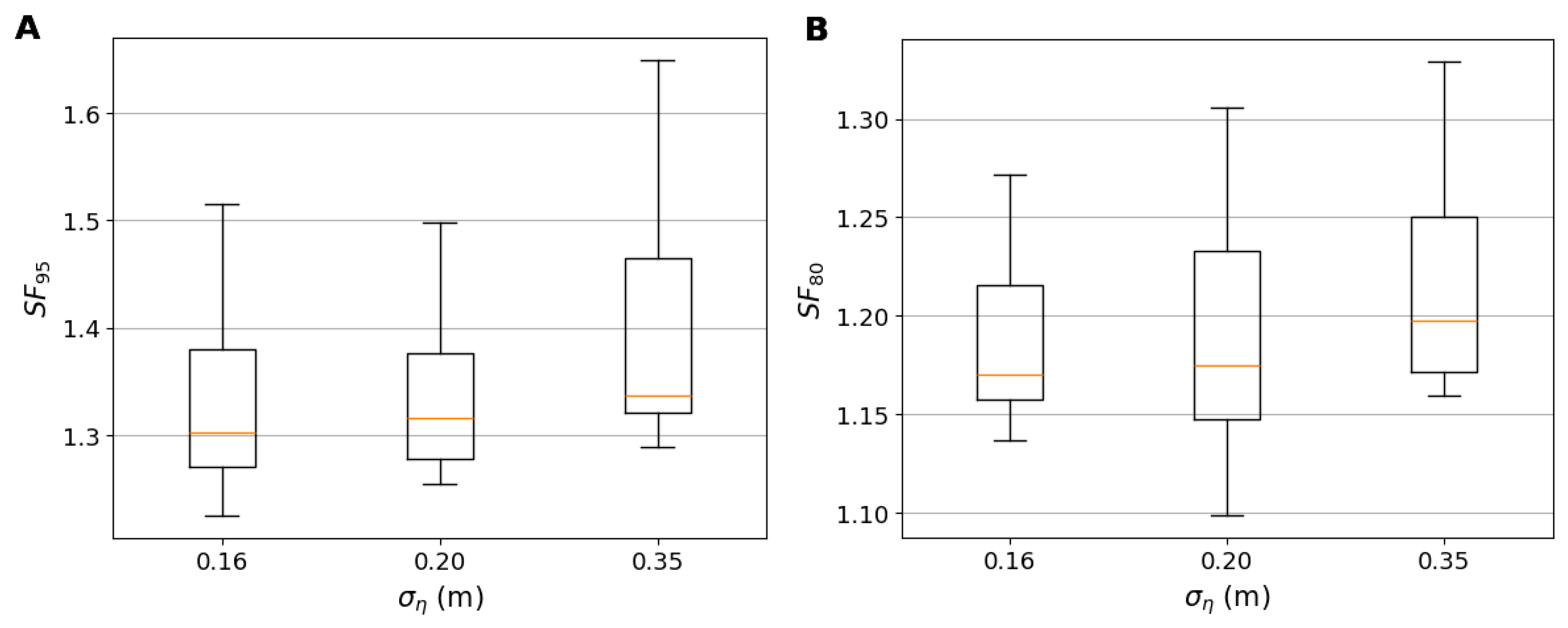
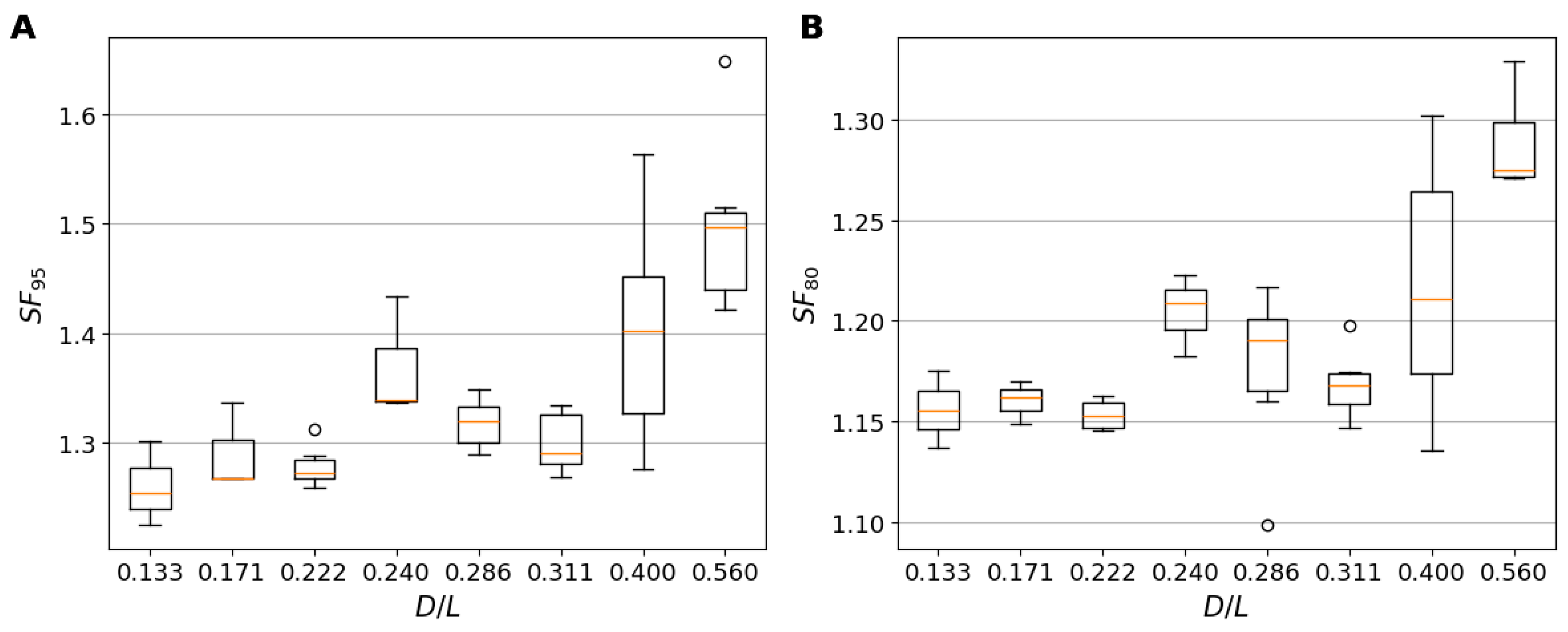
3.4. Parameter Uncertanty Relavence in the Uncertainty Quantification

Figure 11 summarizes the Sobol analysis that we performed to find out which of the uncertain inputs drove the spread of the 95-percentile transmitted wave, H_t,95. Total Sobol indices are variance-based sensitivity metrics that apportion the total output variance to individual inputs and their interactions. Each panel shows the total-order Sobol index of one group of inputs—the still-water level in (a), the significant-wave height in (b), the spectral peak period in (c), and the two coefficients of the model as defined by Equation (3)—plotted against the three tide level uncertainty values examined (0.16, 0.20 and 0.35 m). Because the index measures the fractional contribution of an input (including its interactions) to the variance of the output, values close to unity indicate high influence, whereas values near zero indicate that the parameter is practically irrelevant.

Panel A shows that the Sobol index assigned to the tide increases with tide level uncertainty, which is to be expected. With the smallest tide uncertainty (σ_η = 0.16 m), it accounts for less than ten percent of the variance, but as the uncertainty is increased to σ_η = 0.35 m, its median index rises to about 0.35 and reaches 0.45 in the upper quartile. Its influence is therefore highly non-linear.

Panels B and C trace the opposite trend for the wave parameters. When tide uncertainty is small, the uncertainties in significant wave height H_s and peak period T_p each explain roughly 0.4 of the total wave transmission variance. As the tide uncertainty increases, indices fall steadily, dipping below 0.30 for Hs and falling to around 0.33 for T_p in the scenario with the highest tide uncertainty. This shows that, while the wave climate is very important under conditions of low tide uncertainty, its relative importance is comparable to that of tide uncertainty importance when σ_η = 0.35 m. It is expected that even higher tide uncertainty would produce the most significant uncertainty overall.

Finally, panel D demonstrates that the model’s uncertainty in the slope m and intercept c, used to in Equation (3), has very low significance in terms of the uncertainty of the H_s parameter. Their combined Sobol indices remain below five percent, implying that improving the regression fit will yield little additional gain compared with the effect of reducing environmental uncertainties.

The storm surge also showed very low significance regarding the uncertainty of wave transmission, with a Sobol index below 0.01. This is the case due to the simplistic manner in which it was incorporated into this study. Unfortunately, more precise incorporation would only be possible when performing probabilistic calculations using the framework outlined in Section 2.3 for a specific site and with available measurements.

4. Discussion

This study set out to quantify how parameter uncertainty alters the expected performance of semi-submerged curtain wall breakwaters, which exhibit a structure that is increasingly favored for marina protection in microtidal areas but still designed almost exclusively with deterministic equations. By embedding a modified Wiegel transmission equation inside a Latin Hypercube Sampling (LHS) framework, we showed that required safety factors expand well beyond the values implied by single “mean-value design” waves.

Conventional design practice determines the design incident significant wave height (H_m0,i,mean), peak wave period (T_p), and water levels (commonly mean sea level) as single values with prescribed return periods. Yet, the meta-analysis in Section 2.2 showed that coefficients of variation (CoV) for these variables span up to 0.2, even for well-instrumented sites. Another example is the study by [21], which demonstrates how the coefficient of variation (CoV) could range from 0.05 to 0.20 for H_m0 and reach 0.25 for water level components (including astronomical tides and storm surges), even at locations with extensive instrumentation.

The regression analysis of the LHS results reveals a strong inverse linear relationship between the deterministic transmission coefficient K_t using Equation (3) and the 95th-percentile safety factor SF₉₅ (R ≈ from −0.87 to −0.91). Physically, this implies that breakwaters, whose nominal design already achieves low deterministic transmission (K_t ≤ 0.35), incur a disproportionately high safety factor penalty once wave transmission uncertainty is acknowledged. The effect is most pronounced for the largest tide uncertainty (σ_η = 0.35 m), where the regression slope reaches –1.27 and the intercept reaches 1.91. Under that regime, a design trimmed to K_t = 0.30 requires SF₉₅ ≈ 1.53, whereas a design at K_t = 0.50 needs only SF₉₅ ≈ 1.28. The same inverse trend is visible, though less steep, for σ_η = 0.20 m (slope = –0.88) and σ_η = 0.16 m (slope = –0.94). This confirms that the semi-submerged curtain wall becomes “uncertainty-sensitive” in the performance range that designers often target for marina basins (K_t ≈ 0.30–0.40).

To consider the phenomena itself, the wave transmission mechanism scales non-linearly with the gap ratio D/L —captured by Wiegel-type formulas—producing the familiar S-shaped transmission curve. The transmission curve is very steep for K_t < 0.4 and/or high D/L, becoming increasingly flat for lower higher K_t and/or lower D/L. In the steep low-K_t regime, small uncertainties in the input parameters move the operating point horizontally across the S-curve’s inflection zone, converting input uncertainty. This manifests in relatively large swings in transmitted energy. This is observed in Figure 6, Figure 9 and Figure 10, where lower K_t and higher D/L warrant higher SF₉₅ due to this effect of high sensitivity to input perturbation. Conversely, once the design sits on the relatively flat portion of the S-curve (K_t > 0.4), the same input uncertainty only produces minor changes in the wave power transfer: ∂K_t/∂(·) is small, so the propagated variance is smaller.

For practical purposes, designers may therefore (i) pick the local tidal signal standard deviation that is relevant for the site, (ii) estimate the deterministic K_t from baseline Equation (3), and (iii) apply the above expression to obtain a site-specific SF₉₅. For another example, marina downtime predictions often convert an allowable transmitted height (H_t,lim) into an allowable deterministic K_t by dividing H_t,lim by the long-term significant height H_m0. Using the above relationships in Figure 9 and Figure 10, the probabilistic limit is calculated by K_t,95 = K_t × SF₉₅ and used to calculate the limiting incident wave height H_t,lim/K_t,95 = H_m0,95 to would ensure the H_t,lim inside the marina basin while taking into consideration input parameter uncertainties.

Sobol index analysis decisively points to two parameters as the most significant in influencing the uncertainty of wave transmission. These are H_s and T_p uncertainty when H_s^COV = 0.1 and T_P^COV = 0.08, with both contributing 40% of the total variance in H_t for a low tide level uncertainty of σ_η = 0.16 m. The influence of the uncertainty of tide level during storm events becomes comparable with the wave parameter’s influence at σ_η = 0.35 m. Tide uncertainty becomes significant in relation to wave transmission when σ_η > 0.35 m. On the other hand, model form uncertainty contributes less than 8% of the total variance in H_t. Consequently, improved site characterization—especially of wave and tide parameters—offers greater risk reduction leverage than more sophisticated linear hydrodynamic solvers.

Although the present analysis is applied to a present-day design scenario, semi-empirical projections from the IPCC AR6 indicate that the mean sea level at many temperate-latitude marinas will rise by 0.20–0.35 m under the SSP2-4.5 scenario by 2050 [33]. Our regression, shown in Figure 10 and Figure 11, indicates that a 0.20 m upward drift in the long-term water level would increase the water depth and draft of the curtain breakwater, leaving W/D at the same value but increasing W/L and increasing D/L. This, in turn, increases the SF₉₅ and SF₈₀ in a non-linear fashion depending on the current W/L and D/L values at a specific site. At the same time, an increase in W/L and D/L decreases the deterministic Wiegel wave transmission. Let us take an example a curtain wall optimized today where deterministic K_t = 0.4 (T_p = 3.0 s, W = 2 m, D = 5 m). In a SLR = 0.2 m scenario, the deterministic K_t would decrease to K_t ≈ 0.37 within the lifetime of a typical 30-year marina concession (a ≈ 7.5% decrease in deterministic K_t). The K_t,95 would change from 0.56 to 0.54, and so a ≈ 3.5% decrease in K_t,95 would be observed for the same time period. For a specific site, the uncertainty in sea level rise could be directly incorporated into the Latin Hypercube framework for site-specific estimation. In short, a small reduction in wave transmission is anticipated due to rising sea levels.

This study is limited by its oversimplified storm surge quantification, suggested by [11,27,28], in the uncertainty quantification. This is particularly relefant for high-surge areas like those prone to tropical cyclones. For these situations, we recommend using the site-specific uncertainty quantification of environmental parameters to determine site-specific safety factors (SF₈₀ and SF₉₅).

5. Conclusions

This work provides the first quantitative reliability-based framework for semi-submerged curtain wall breakwaters—a system that, despite its growing popularity for marina protection in microtidal basins, is still designed almost exclusively with deterministic equations, mostly employing Wigel-based theory [13]. By embedding a modified Wiegel transmission formula in a Latin Hypercube Sampling loop that explicitly accounts for the measured coefficients of variation in significant wave height, peak period, tide level, and storm surge, as well as model uncertainty, we showed that the conventional “mean-value” design can understate the 95% non-exceedance risk by as much as 50% (SF₉₅ = 1.5). A simple regression envelope, expressed as SF₉₅ = 1.91 − 1.27 × K_t for σ_η = 0.35 m (and analogous lines for smaller tide uncertainty), now enables designers to translate any deterministic transmission target into a 95% non-exceedance margin in a single calculation step.

Physically, the results trace directly to the S-shaped draft-sensitivity embedded in Wiegel’s power-balance model: when the nominal design sits on the steep part of that curve (typical target range K_t ≈ 0.0–0.40), even modest uncertainty in H_m0, T_p, or tide level pushes the operating point widely across the inflection zone, amplifying variance in transmitted wave power and inflating the required safety factor. Conversely, once the curtain is shallow enough to place the design on the flatter asymptote (K_t ≳ 0.45), the same environmental scatter only produces marginal changes in transmission, and SF₉₅ naturally collapses toward unity. Sobol decomposition confirmed that uncertainties in H_m0 and T_p each account for roughly 40% of the variance in H_t during situations of small tide level uncertainty, with tide uncertainty only becoming equally important when tide level uncertainty exceeds 0.30 m. Model form uncertainty, by contrast, contributes less than 8%, implying that the improved characterization of wave–tide statistics yields greater risk reduction leverage than successively higher-order hydrodynamic solvers.

References

1. Hoàng Thái Dương, V.; Zemann, M.; Oberle, P.; Seidel, F.; Nestmann, F. Investigating Wave Transmission through Curtain Wall Breakwaters under Variable Conditions. J. Coast. Hydraul. Struct. 2023, 2, 2022. [Google Scholar] [CrossRef]
2. Subekti, S.; Shulhany, A. Transmission and reflection of waves on curtain wall breakwater. Tek. J. Sains Dan Teknol. 2021, 17, 100–105. [Google Scholar] [CrossRef]
3. Carevic, D.; Bujak, D.; Potočki, K.; Drašković, J. Wave Transmission Below Breakwaters with Semi- Immersed Curtain. In Proceedings of the 16h International Symposium on Water Management and Hydraulic Engineering, Skopje, North Macedonia, 5–7 September 2019. [Google Scholar]
4. Bartolić, I.; Lončar, G.; Bujak, D.; Carević, D. The Flow Generator Relations for Water Renewal through the Flushing Culverts in Marinas. Water 2018, 10, 936. [Google Scholar] [CrossRef]
5. Lončar, G.; Bartolić, I.; Bujak, D. Contribution of Wind and Waves in Exchange of Seawater through Flushing Culverts in Marinas. Teh. Vjesn.-Tech. Gaz. 2018, 25, 1587–1594. [Google Scholar] [CrossRef]
6. Karimi, M.S.; Mohammadi, R.; Raisee, M.; Hendrick, P.; Nourbakhsh, A. Robust optimization of a marine current turbine using a novel robustness criterion. Energy Convers. Manag. 2023, 295, 117608. [Google Scholar] [CrossRef]
7. Ni, P.; Li, J.; Hao, H.; Xia, Y.; Du, X. Stochastic dynamic analysis of marine risers considering fluid-structure interaction and system uncertainties. Eng. Struct. 2019, 198, 109507. [Google Scholar] [CrossRef]
8. Burcharth, H.F. Uncertainty Related to Environmental Data and Estimated Extreme Events: PIANC PTC II Working Group 12, Report of Subgroup B; Aalborg Universitetsforlag: Aalborg, Denmark, 1992. [Google Scholar]
9. PIANC (Ed.) Breakwaters with Vertical and Inclined Concrete Walls: Report of Working Group 28 of the Maritime Navigation Commission; PIANC General Secretariat: Bruxelles, Belgium, 2003; ISBN 978-2-87223-139-3. [Google Scholar]
10. Schüttrumpf, H.; Kortenhaus, A.; Peters, K.; Fröhle, P. Expert judgement of uncertainties in coastal structure design. In Proceedings of the Coastal Engineering 2006, San Diego, CA, USA, 3–8 September 2006; World Scientific Publishing Company: San Diego, CA, USA, 2007; pp. 5267–5278. [Google Scholar]
11. Suh, K.-D.; Kim, S.-W.; Mori, N.; Mase, H. Effect of Climate Change on Performance-Based Design of Caisson Breakwaters. J. Waterw. Port Coast. Ocean Eng. 2012, 138, 215–225. [Google Scholar] [CrossRef]
12. Eurotop EurOtop II. European Overtopping Manual—Wave Overtopping of Sea Defences and Related Structures: Assessment Manual; Envrionment Agency: Rotherham, UK, 2018.
13. Wiegel, R.L. Transmission of Waves Past a Rigid Vertical Thin Barrier. J. Waterw. Hourbours Div. 1960, 86, 1–12. [Google Scholar] [CrossRef]
14. Kriebel, D.L.; Bollman, C.A.; Billy, L.E. Wave transmission past vertical wave barriers. In Proceedings of the 25th International Conference on Coastal Engineering, Orlando, FL, USA, 2–6 September 1996. [Google Scholar]
15. Yu, Y.; Guo, Z.; Ma, Q. Transmission of Water Waves under Multiple Vertical Thin Plates. Water 2018, 10, 517. [Google Scholar] [CrossRef]
16. Lee, C.-E.; Kwon, H.J. Reliability analysis and evaluation of partial safety factors for random wave overtopping. KSCE J. Civ. Eng. 2009, 13, 7–14. [Google Scholar] [CrossRef]
17. Tsimopoulou, V. Probabilistic Design of Breakwaters in Shallow, Hurricane-Prone Areas. Master’s Thesis, Delft University of Technology, Delft, The Netherlands, 2011. [Google Scholar]
18. Oumeraci, H.; Allsop, W.; Groot, M.; Crouch, R.; Vrijling, J. Proverbs: Probabilistic Design Tools for Vertical Breakwaters; CRC Press: Boca Raton, FL, USA, 2001. [Google Scholar]
19. Doan, N.S.; Huh, J.; Mac, V.H.; Kim, D.; Kwak, K. Probabilistic Risk Evaluation for Overall Stability of Composite Caisson Breakwaters in Korea. J. Mar. Sci. Eng. 2020, 8, 148. [Google Scholar] [CrossRef]
20. Oumeraci, H. Proverbs: Probabilistic Design Tools for Vertical Breakwaters; CRC Press: Boca Raton, FL, USA, 1999; Volume 2. [Google Scholar]
21. Kortenhaus, A. Probabilistische Methoden für Nordseedeiche; Technical University of Braunschweig: Braunschweig, Germany, 2003. [Google Scholar] [CrossRef]
22. Katalinić, M.; Parunov, J. Uncertainties of Estimating Extreme Significant Wave Height for Engineering Applications Depending on the Approach and Fitting Technique—Adriatic Sea Case Study. J. Mar. Sci. Eng. 2020, 8, 259. [Google Scholar] [CrossRef]
23. Kim, S.-W.; Suh, K.-D. Performance Analysis of Vertical Breakwaters Designed by Partial Safety Factor Method. J. Coast. Res. 2013, 65, 296–301. [Google Scholar] [CrossRef]
24. Suh, K.-D.; Kwon, H.-D.; Lee, D.-Y. Some statistical characteristics of large deepwater waves around the Korean Peninsula. Coast. Eng. 2010, 57, 375–384. [Google Scholar] [CrossRef]
25. Bujak, D.; Loncar, G.; Carevic, D.; Kulic, T. The Feasibility of the ERA5 Forced Numerical Wave Model in Fetch-Limited Basins. J. Mar. Sci. Eng. 2023, 11, 59. [Google Scholar] [CrossRef]
26. Bujak, D.; Bogovac, T.; Carević, D.; Miličević, H. Filling Missing and Extending Significant Wave Height Measurements Using Neural Networks and an Integrated Surface Database. Wind 2023, 3, 151–169. [Google Scholar] [CrossRef]
27. Takagi, H.; Goda, Y. A Reliability Design Method of Caisson Breakwaters with Optimal Wave Heights. Coast. Eng. J. 2000, 42, 357–387. [Google Scholar] [CrossRef]
28. Kim, T.-M.; Takayama, T. Computational Improvement for Expected Sliding Distance of a Caisson-Type Breakwater by Introduction of a Doubly-Truncated Normal Distribution. Coast. Eng. J. 2003, 45, 387–419. [Google Scholar] [CrossRef]
29. Karatzetzou, A. Uncertainty and Latin Hypercube Sampling in Geotechnical Earthquake Engineering. Geotechnics 2024, 4, 1007–1025. [Google Scholar] [CrossRef]
30. Hajihassanpour, M.; Kesserwani, G.; Pettersson, P.; Bellos, V. Sampling-Based Methods for Uncertainty Propagation in Flood Modeling Under Multiple Uncertain Inputs: Finding Out the Most Efficient Choice. Water Resour. Res. 2023, 59, e2022WR034011. [Google Scholar] [CrossRef]
31. PIANC. Seismic Design Guidelines for Port Structures; PIANC: Brussels, Belgium, 2001. [Google Scholar]
32. U.S. Army Corps of Engineers. Coastal Engineering Manual; U.S. Army Corps of Engineers: Washington, DC, USA, 2002. [Google Scholar]
33. Intergovernmental Panel on Climate Change (IPCC) (Ed.) Summary for Policymakers. In Climate Change 2021—The Physical Science Basis: Working Group I Contribution to the Sixth Assessment Report of the Intergovernmental Panel on Climate Change; Cambridge University Press: Cambridge, UK, 2023; pp. 1–2. ISBN 978-1-009-15788-9. [Google Scholar]
Figure 1. Definition sketch of irregular wave transmission beneath semi-submerged curtain breakwater.
Infrastructures 10 00144 g001
Figure 2. Workflow of uncertainty quantification study and safety parameter calculation; orange arrows show the pathway for probabilistic calculations and green arrows for deterministic calculations.
Infrastructures 10 00144 g002
Figure 3. Comparison of measured wave transmission coefficients (Kt,Measured) with theoretical predictions from Wiegel’s power transmission theory (Kt,Wiegel) and modified power transmission model (Kt,Mod.Power).
Infrastructures 10 00144 g003
Figure 4. Comparison between measured transmission coefficients of irregular waves and predictions by Wiegel’s Equation (1). Blue dots represent 72 individual laboratory data points from [3]. Red line is least-squares linear regression (Kt,Measured = 0.845*Kt,Wiegel + 0.027; R = 0.98). Green lines denote ± 1 standard deviation of residuals, and blue lines indicate 95% confidence interval for regression.
Infrastructures 10 00144 g004
Figure 5. Influence of astronomical tide-defined sea level uncertainty on design safety factor. Panel (A) shows box-and-whisker plots of 95th-percentile safety factor (SF95); panel (B) shows the corresponding 80th-percentile safety factor (SF80); both are evaluated for three representative tidal uncertainty, namely 0.16 m, 0.20 m, and 0.35 m.
Infrastructures 10 00144 g005
Figure 6. Effect of relative draft W/L0 on safety factor: panel (A) shows 95% non-exceedance safety factor SF95, and panel (B) shows 80% factor SF80.
Infrastructures 10 00144 g006
Figure 7. Effect of relative depth D/L0 on safety factor: panel (A) shows 95% non-exceedance safety factor SF95, and shows panel (B) 80% factor SF80.
Infrastructures 10 00144 g007
Figure 8. Effect of relative depth W/D on safety factor; panel (A) shows 95% non-exceedance safety factor SF95, and panel (B) shows 80% factor SF80.
Infrastructures 10 00144 g008
Figure 9. Relationship between deterministic transmission coefficient using Equation (3) and 80th-percentile safety factor for three astronomical tide level uncertainty (ση) scenarios.
Infrastructures 10 00144 g009
Figure 10. Relationship between deterministic transmission coefficient using Equation (3) and 95th-percentile safety factor for three scenarios featuring astronomical tide level uncertainty (ση).
Infrastructures 10 00144 g010
Figure 11. Total order Sobol indices, identifying which uncertain inputs control variability of transmitted wave height, Ht.m0; (A) shows indices for Tide uncertainty; (B) shows indices for Hm0 uncertainty; (C) shows indices for Tp uncertainty; (D) shows indices for model uncertainty.
Infrastructures 10 00144 g011