Dynamic Modulus Regression Models for Cold Recycled Asphalt Mixtures

Abstract

Cold recycling is an advantageous technique from economic and environmental perspectives for asphalt pavement rehabilitation, interventions, and maintenance. This work covered the investigation of dynamic modulus (|E*|) test models and their effects on cold recycled asphalt mixture (CRAM) |E*| data fitting, considering different mixture parameters such as asphalt binder type and content, active filler type and content, aggregate gradation, reclaimed asphalt pavement content, and curing conditions. Multiple mixtures from a dynamic modulus test database were fitted using six different regression models and the results were analyzed by means of different residuals analysis. Finally, the effects of CRAM composition on |E*| data were graphically assessed. For the analyzed specimens, two models were found to be the most adequate for CRAM’s |E*| data regression. The analysis of CRAM composition showed a strong relation between the compaction method and the stiffness of CRAMs.

1. Introduction and Background

Cold asphalt pavement recycling is on the rise for rehabilitation, interventions, and maintenance of asphalt pavements, mainly due to its economic and environmental benefits [1]. The technique consists of creating a new mixture from the incorporation of milled material known as reclaimed asphalt pavement (RAP). The mixture is then stabilized by asphalt emulsion or foamed asphalt, and, when necessary, Portland cement, hydrated lime, or other filler are also added. The recycled mixture is commonly used as a base layer with an overlay of asphalt concrete (AC) for protection.

Cold recycled asphalt mixtures (CRAM) may present complex mechanical behavior, and it is challenging to predict the behavior of such material along its service life. CRAM shows stress-state dependence, i.e., its stiffness is dependent on the confining stresses [2,3,4,5,6,7]. At the same time, since CRAM composition includes asphalt binder, it behaves as an asphaltic material, in which its stiffness is also dependent on load frequency and material temperature [5,8,9,10,11]. Also, many other factors can impact the CRAM mechanical behavior, such as RAP source and content, stabilizing agent type and content, active filler type and content, curing process, and moisture content, among others [4,12,13,14,15,16,17]. The difficulties in predicting the behavior and performance of this material impair the adoption of this technique by some transportation agencies and delay the dissemination of cold recycling practices.

The dynamic modulus test results provide important information for asphalt mixture characterization and, consequently, for the pavement design process. The test is described by AASHTO T 342 [18], in which cylindrical compacted asphalt specimens are subjected to a sinusoidal (haversine) axial compressive loading under temperature and frequency sweeps, while the on-specimen deformation is measured. The dynamic modulus test results are usually expressed as a regression model of the |E*| (dynamic modulus) vs. reduced frequency (dynamic modulus master curve).

A literature review of dynamic modulus master curve regression models for asphalt mixtures tests is presented in

Table 1. Asphalt mixture |E*| master curve models.

MATHEMATICAL MODELS
Author	Regression Model	Parameters
Pellinen et al., 2002 [20]	Sigmoidal $\log \left(\right|E^{\ast }\left|\right)=\delta +{\displaystyle \frac{\alpha }{1+e^{\beta -\gamma \log \left(\omega \right)}}}$	$\delta =minimunmodulusvalue$ $\propto =spanofmodulusvalues$ $\beta ,\gamma =shapeparameters$ $\omega =angularreducedfrequency$
Seo et al., 2007 (*) [21]	$\log \left(\right|E^{\ast }\left|\right)=a+{\displaystyle \frac{b}{1+\frac{1}{e^{c+d\log \left(\omega \right)}}}}$	$a,b,c,d=regressioncoefficients$ $\omega =angularreducedfrequency$
Rowe et al., 2008 [22]	Richard’s model or generalized sigmoidal $\log \left(\right|E^{\ast }\left|\right)=\delta +{\displaystyle \frac{\alpha }{{(1+{\lambda e}^{\beta +\gamma \log \left(\omega \right)})}^{1/\lambda }}}$	$\delta =minimunmodulusvalue$ $\propto =spanofmodulusvalues$ $\beta ,\gamma =shapeparameters$ $\omega =angularreducedfrequency$ $\lambda =generalizationparameter$
AASHTO 2017 [23]	AASHTO R84-17—Hirsch model $\log \left(\right|E^{\ast }\left|\right)=\delta +{\displaystyle \frac{(Max-\delta )}{1+e^{\beta +\gamma \log \left(f_r\right)}}}$	$Max=limitingmaximummodulus$ $\delta ,\beta ,\gamma =fittingparameters$ $f_r=reducedfrequency$
PHYSICALLY SIGNIFICANT PARAMETERS MODELS
Christensen 1998 [24]	Christensen–Anderson–Marasteanu (CAM) $\left|E^{\ast }\right|=E_g{\left[1+{\left({\displaystyle \frac{\omega }{t_c}}\right)}^{\nu }\right]}^{-{\displaystyle \frac{w}{\nu }}}$	$E_g=glassymodulus\left(\omega \to \infty \right)$ $\omega =angularreducedfrequency$ $w,\nu ,t_c=shapeparameters$
Zeng et al., 2001 [25]	Modified CAM $\left|E^{\ast }\right|=E_e+{\displaystyle \frac{E_g-E_e}{{\left[1+{\left(\frac{f_c}{f\prime }\right)}^k\right]}^{\frac{m_c}{k}}}}$	$E_e=equilibriummodulus\left(\omega \to 0\right)$ $E_g=glassymodulus\left(\omega \to \infty \right)$ $k,m_c=shapeparameters$ $f_c=locationparameter$ $f\prime =reducedfrequency$
Falchetto et al., 2021 [26]	SCM $log\left|E^{\ast }\right|={logE}_g+{\displaystyle \frac{w}{\nu }}{\displaystyle \frac{1}{{\left[1+e^{zlog\omega +t_c}\right]}^{\frac{1}{v}}}}$	$E_g=glassymodulus(\omega \to \infty )$ $w,\nu ,t_c,z=shapeparameters$ $\omega =angularreducedfrequency$
MECHANICAL ANALOG MODELS
Sayegh 1965 [27]	Huet–Sayegh $\left|E^{\ast }\right|=E_0+{\displaystyle \frac{E_1}{1+{\delta \left(i\omega \tau \right)}^{-k}{+\left(i\omega \tau \right)}^{-h}}}$	$E_0=equilibriummodulus\left(\omega \to 0\right)$ $E_1=glassymodulus\left(\omega \to \infty \right)$ $\delta =shapeparameters;i=\sqrt{-1}$ $\omega =angularreducedfrequency$ $\tau =characteristictime$ $\left(temperaturedependent\right)$ $k,h=dimensionlessparameters$ $\left(fromparabolicelements\right)$
Havriliak, Negami 1966 [28]	Havriliak–Negami (HN) $\left|E^{\ast }\right|=E_{\infty }+{\displaystyle \frac{E_0-E_{\infty }}{{\left[1+{\left(i\omega \tau \right)}^{\alpha }\right]}^{\beta }}}$	$E_0=equilibriummodulus\left(\omega \to 0\right)$ $E_{\infty }=glassymodulus\left(\omega \to \infty \right)$ $i=\sqrt{-1}$ $\omega =angularreducedfrequency$ $\tau =characteristictime$ $\left(temperaturedependent\right)$ $\alpha ,\beta =shapeparameters$
Olard, Di Benedetto 2003 [29]	2S2P1D model $\left|E^{\ast }\right|=E_{\infty }+{\displaystyle \frac{E_0-E_{\infty }}{1+{\delta \left(i\omega \tau \right)}^{-k}{+\left(i\omega \tau \right)}^{-h}+{\left(i\omega \beta \tau \right)}^{-1}}}$	$E_0=equilibriummodulus\left(\omega \to 0\right)$ $E_{\infty }=glassymodulus\left(\omega \to \infty \right)$ $\delta ,\beta =shapeparameters;i=\sqrt{-1}$ $\omega =angularreducedfrequency$ $\tau =characteristictime$ $\left(temperaturedependent\right)$ $k,h=dimensionlessparameters$ $\left(fromparabolicelements\right)$

^(*) these authors may not be the model creators, but they were the oldest references found using this model.

, which shows the most used models in the past years and that can be divided into three parts: (i) mathematical models, (ii) physically significant parameters models, and (iii) mechanical analog models (or rheological models) [19]. The mechanical analog models are based on Kelvin–Voigt and Maxwell’s generalized models.

The mechanical analog models require many parameters to be determined, and this is the reason for their limited use [30]. These models generate master curves that are based on the real mechanical and rheological behaviors of the materials, derived from physical elements [29]. The other models are more based on statistical analysis, i.e., the results of |E*| are fitted through optimization of the regression parameters.

The models indicated in the review are typically used in the literature to describe the rheological behavior of asphaltic materials. Each model was developed to help address limitations from previous models, including better predictions of the low-temperature modulus of asphalt mixtures, providing a more general application for fitting asphalt mixture and asphalt binder moduli values using a single analytical function, or allowing for a more computer-efficient calculations when implemented in numerical solutions for pavement response and/or performance analyses. Although discussing these models’ particularities is outside of the scope of this study, they allow practitioners to translate the measured |E*| data into an analytical form that can be further used in pavement performance simulations for analysis and design.

The literature review that led to Table 1 construction indicates that the mathematical models are the most used for asphalt mixture |E*| master curve creation. Mathematical models are the most frequent in academic research and it is the main model adopted by agencies [5,31,32,33,34].

Regarding Cold In-Place Recycling with Foamed Bitumen (FB-CIR), the dynamic modulus (sigmoidal fitting model) results revealed that mixtures exhibit clear viscoelastic behavior, characterized by significant frequency dependence and temperature sensitivity, with modulus values decreasing at lower frequencies and higher temperatures [11].

The dynamic modulus and storage modulus master curves (Generalized Sigmoidal and Huet–Sayegh models) revealed minimal differences between the two emulsified-asphalt cold recycled mixtures (ECRM) evaluated, despite variations in RAP content and production methods, while the loss modulus master curve effectively distinguished between the mixtures, highlighting ECRM with higher effective binder content [34].

Currently, the use of |E*| master curve models is commonly used to represent the results of |E*| tests in a graphical way smearing the temperature and frequency dependency into a single variable named reduced frequency. However, the |E*| master curve models can also be used for pavement analysis and design, as implemented in multiple softwares, such as FlexPAVE^TM V1.1, 3D-Move V2.1, AASHTOWare^® Pavement ME V.2.2.6, and ViscoRoute V2.0. Some of these softwares use |E*| raw data without the use of fitting models (e.g., 3D-Move). FlexPAVE^TM uses a Prony series and a two-spring, two-parabolic element, and one dashpot (2S2P1D) model, whereas ViscoRoute V2.0 relies on the Huet–Sayegh model for |E*| characterization. Even though several regression models can be used to fit the data, not much has been discussed on their adequacy for CRAM. The pursuit of the most adequate models can be beneficial to pavements analysis and design from viscoelastic analysis software.

Considering that |E*| master curve models also have not yet been evaluated for CRAM, this study aims to investigate the suitability of different CRAM’s |E*| master curve models through the analysis of an extensive |E*| test database obtained from previous research projects. Hence, research efforts were spent on the statistical analysis of the models, and the conclusions were based on the models’ adequacy and goodness of fit. Additionally, this work investigated if there are any correlations between the model selection and CRAM’s type/content of active filler and asphalt binder. Finally, an analysis of the effects of CRAM’s composition on |E*| data was performed. Figure 1 summarizes the work scope of this paper.

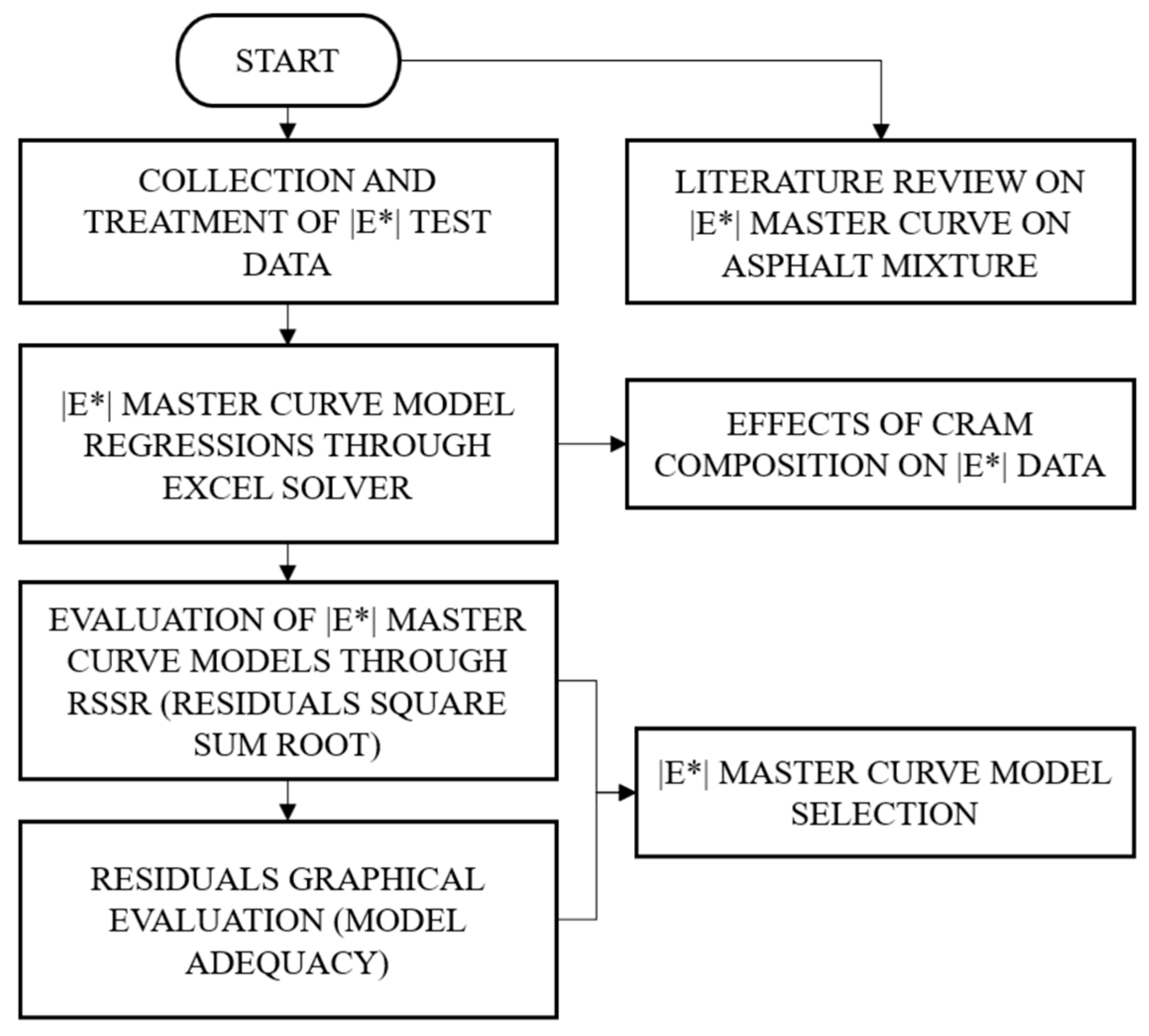
2. Materials and Methods

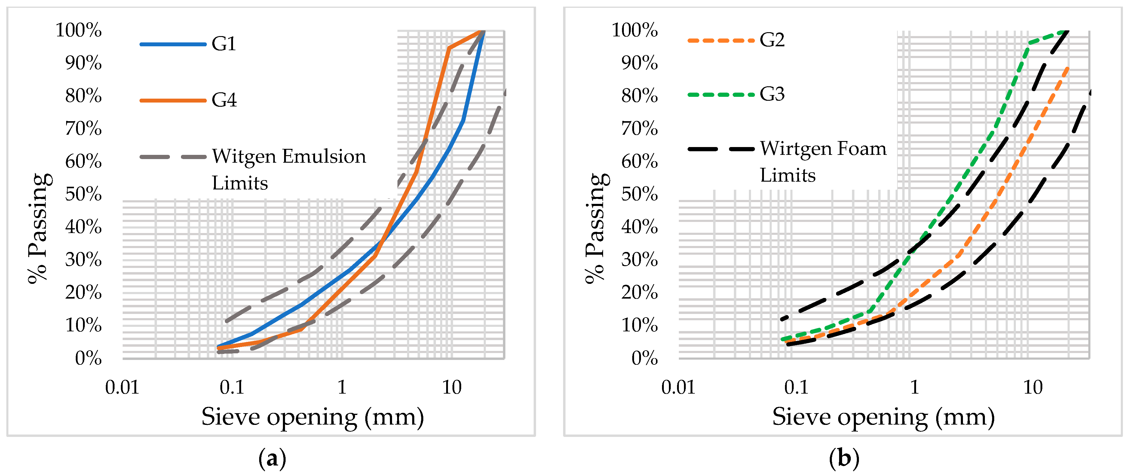
2.1. Materials

A database of |E*| test results was used to determine the model that best fits the CRAM’s |E*| measured data using a statistical approach. To simplify specimens’ identification, a general terminology was adopted and defined as “Gx-yBzF_Cw_R” and the detailed description is presented in Figure 2.

As an example, if a given mixture is identified by the terminology of “G1-2E1C_C1_1”, this means that the mix is comprised by gradation 1 (G1), 2% of emulsion (2E), 1% of Portland cement (1C), following curing method 1 (C1), relative to the replicate specimen number 1. The mixtures evaluated in this study were evaluated in previous studies for different purposes as part of a group task force to investigate the mechanical behavior of cold recycled asphalt mixtures. Additional information on the mixture’s characteristics presented herein is available elsewhere [5,35,36].

The evaluated specimens and the corresponding number of replicates are presented in

Table 2. CRAM replicates and main information.

Specimen ID	Mineral Skeleton	Air Void Content (%)	Curing	Compaction	Replicates
G1-2E1C_C1	85% RAP + 15% crushed stone	15.8	7 days—40 °C	Gyratory until locking point	13
G1-2E1H_C1					3
G1-2E00_C1					2
G1-2E2C_C1					3
G1-2E2H_C1					3
G2-2.2F1H_C1	89.9% RAP + 10.1% crushed stone	-	7 days—40 °C	Vibratory **	3
G3-3F2C_C2	69.4% RAP + 30.6% crushed stone	-	28 days—40 °C	Vibratory **	2
G3-3F2C_C3			40 °C—until 60% OMC *	Modified Proctor	2
G4-3E2C_C4	100% RAP	-	3 days—60 °C	Modified Proctor	2
G4-3E2C_C2			28 days—40 °C	Vibratory **	2
Total					35

* OMC stands for Optimum Moisture Content = the compaction’s moisture content. ** Bosch GSH 11 VC vibratory hammer (1700 W), 30 kg weight—2 layers (5 s each).

along with the mixture’s mineral skeleton composition and specimens’ average air void content. The aggregate gradation is shown in Figure 3, with the Wirtgen’s recommended gradation limits for CRAMs [37]. Aggregate gradations do not align with Wirtgen’s limits, and this is related to RAP gradation.

Compaction methods and specimen numbers were based on data availability. The specimens were submitted to different curing conditions, which consisted of oven drying the specimens for different durations at different temperatures, as presented in Table 2. More information on the curing procedure and RAP source (variable source) is available elsewhere [5,35,36]. However, it is important to highlight that, except for the curing condition C3 (60% OMC), the specimens were in a “dryer state” compared to the field content of the initial years after the construction of the pavement [38]. Moloto [38] presents a comprehensive summary of different field curing protocols that vary in terms of curing time (from 0 to ~220 days) and residual moisture (from ~50% to ~82% of OMC). Even though several curing procedures exist for different types of CRAMs, the procedures used in this study aimed to achieve the final curing stage, in which the mixture exhibits the highest structural bearing capacity.

The |E*| test followed the AASHTO T 342 [18] procedure, although it was initially intended for hot asphalt mixtures. This procedure has shown to be also applicable for cold recycled asphalt mixture characterization [5,8,9]. The tests were not conducted at −10 °C and 54 °C temperatures, as those are not typical temperatures in base layers of Brazilian pavements. At 37.8 °C, the specimens showed significantly low stiffness, and the test’s load amplitude was as low as 300 N. Also, Kuchiishi [39] found that the 54 °C temperature can trigger the RAP residual binder reactivation and change the CRAM’s mechanical behavior. Therefore, the test temperatures were: 4.4 °C, 21.1 °C, and 37.8 °C.

The |E*| results were then shifted to a reference temperature of 21.1 °C by means of the shift factor equation defined by the polynomial function shown in Equation (1). The reduced frequency calculation is given by Equation (2). Thus, it was possible to represent and analyze the |E*| data at a single temperature.

$$\log \left(a_T\right)={\alpha }_1{T}^2+{\alpha }_{2}T+{\alpha }_3$$

(1)

$$\log \left(f_r\right)=\log \left(f\right)+\log \left(a_T\right)$$

(2)

α_T is the shift factor at a temperature T; α₁, α_2, and α₃ are the shift factor polynomial equation coefficients; T is the temperature; and f is the test frequency.

2.2. Method

From the literature review presented in Table 1, six (out of ten) different models were selected for the analysis: (i) the Sigmoidal model (Equation (3)); (ii) Seo et al.’s Sigmoidal model (Equation (4)); (iii) Richard’s model or Generalized Sigmoidal model (Equation (5)); (iv) the Christensen–Anderson–Marasteanu (CAM) model (Equation (6)); (v) the Modified CAM model (Equation (7)); (vi) the SCM model (Equation (8)). The description of each equation’s parameter was previously presented in Table 1. Four models were discarded, and the reasons are as follows. The Hirsch model was not selected due to its similarity to the Sigmoidal model—both models produce the same fit. All three mechanical analog models were not assessed in this work. The main reason is that these models have physical meaning. Therefore, these models aim to represent the asphalt mixture behavior through a mechanical analogy, and regression analysis quality is not the main objective (although it is still an objective of these models). Hence, it would be counterproductive to compare these models’ adequacy and goodness of fit.

$$\log \left(\right|E^{\ast }\left|\right)=\delta +{\displaystyle \frac{\alpha }{1+e^{\beta -\gamma \times \log \left(\omega \right)}}}$$

(3)

$$\log \left(\right|E^{\ast }\left|\right)=a+{\displaystyle \frac{b}{1+\frac{1}{e^{c+d\times \log \left(\omega \right)}}}}$$

(4)

$$\log \left(\right|E^{\ast }\left|\right)=\delta +{\displaystyle \frac{\alpha }{{(1+{\lambda e}^{\beta +\gamma \times \log \left(\omega \right)})}^{1/\lambda }}}$$

(5)

$$\left|E^{\ast }\right|=E_g{\left[1+{\left({\displaystyle \frac{\omega }{t_c}}\right)}^{\nu }\right]}^{-{\displaystyle \frac{w}{\nu }}}$$

(6)

$$\left|E^{\ast }\right|=E_e+{\displaystyle \frac{E_g-E_e}{{\left[1+{\left(\frac{f_c}{\omega }\right)}^k\right]}^{\frac{m_c}{k}}}}$$

(7)

$$log\left|E^{\ast }\right|={logE}_g+{\displaystyle \frac{w}{\nu }}\times {\displaystyle \frac{1}{{\left[1+e^{z\times log\omega +t_c}\right]}^{\frac{1}{v}}}}$$

(8)

2.3. Statistical Analysis

The linear least-squares method (LSM) is a frequently used tool in linear regression analysis. This method aims to minimize the sum of the regression’s residuals’ squares. Residuals are defined as the difference between the observed values (real data) and the estimated values (modeled data). Therefore, this method is oftentimes used to minimize the residual sum of squares and provide a better estimation of the measured data. Since this is a simple and direct method, linear regression’s data fitting is largely performed by means of LSM.

Although Equations (3)–(8) are nonlinear functions (i.e., the relation between |E*| and ω is not linear), they are linearizable functions through appropriate transformations. Therefore, LSM is still applicable and was performed in this study using Excel’s Solver tool, which is a very common approach. Seed values for the model coefficients (e.g., α, β, γ) are initially chosen based on the fitting coefficients of asphalt mixtures presented in the literature and the Solver tool runs iterations changing the coefficients to reduce the sum of the regression’s residuals’ squares.

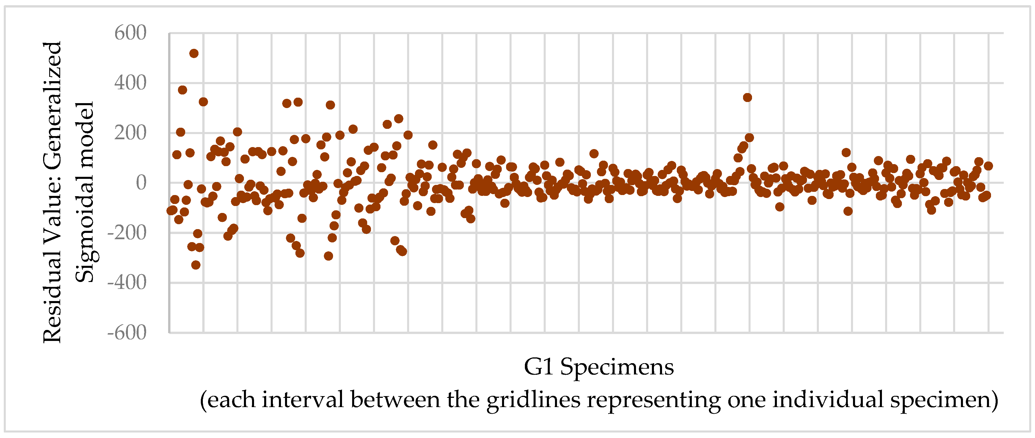
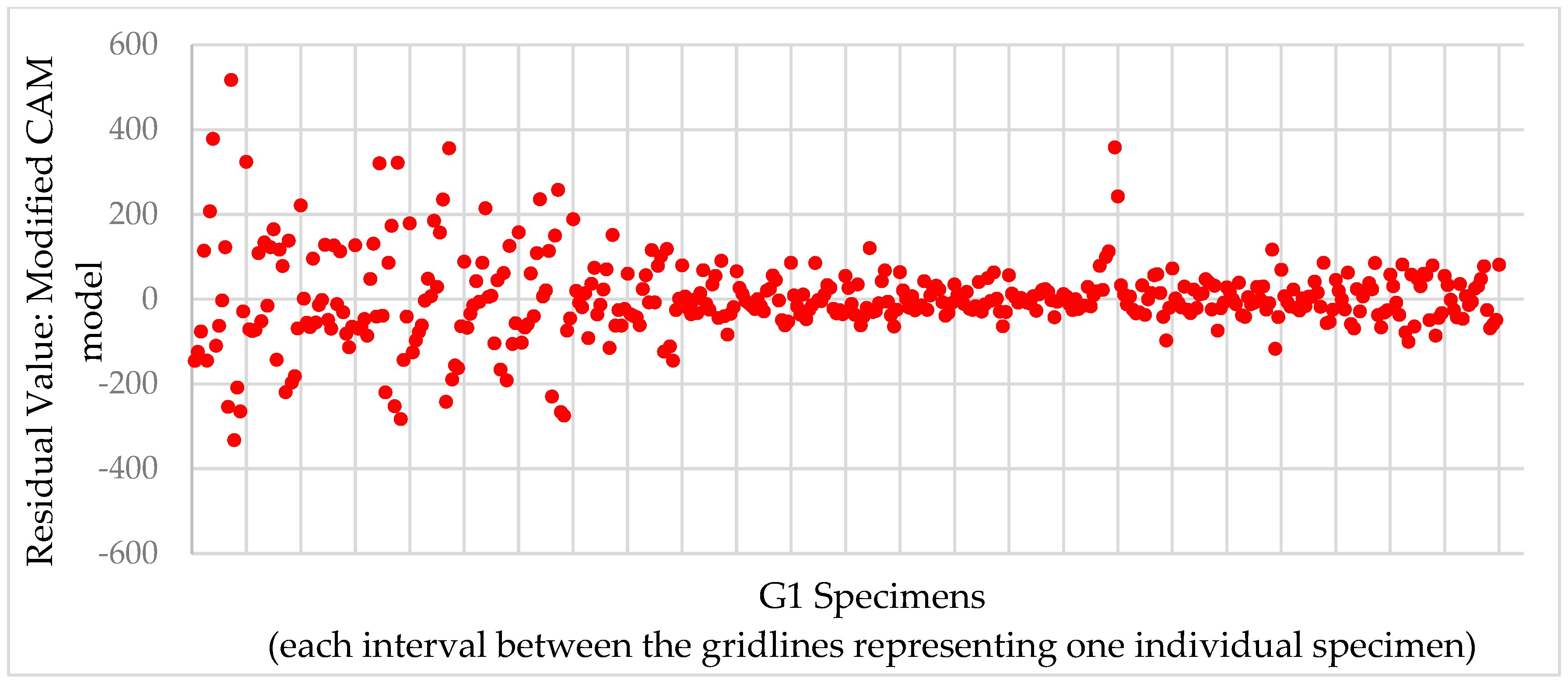
3. Results and Discussions

After running the linear least-squares method (LSM) using Excel’s Solver tool, the optimized regression coefficients were found for each model; consequently, the |E*| master curve regression models were proposed for each specimen.

The coefficient of determination (R²), although largely used to evaluate linear regressions, is inappropriate for evaluating nonlinear models [40]. For example, the R² value of the specimen G1-2E1C_08 was equal to 0.9979 for all regression models (Equations (3)–(8)), and no conclusion could be extracted from that. Models’ adequacy was assessed by means of a simple and effective residual transformation, which is defined in Equation (9), where $r_1,r,\dots ,r_n$ are the fitted residual values.

$$RSSR=\sqrt{\sum _{i=1}^n{r}_i^2}$$

(9)

The analysis of residuals (or their transformations) is an extremely useful tool to detect inadequacies of the regression model [41]. RSSR is an acronym for Residuals Square Sum Root. Lower RSSR values are associated with better-fitted regressions, i.e., lower values for the residuals are obtained (best agreement between observed and modeled values). RSSR itself does not provide an absolute quality assessment of regressions, such as R², but it is efficient in comparing different models, which is the primary objective of this study.

In this sense, the Akaike Information Criterion (AIC) [42] or the Bayesian Information Criterion (BIC) [43] can be used to compare the different master curve models adequacy. AIC and BIC are the most common criterion tools used for nonlinear model selection [41]. Both AIC and BIC penalize an excessive number of independent variables (overfitting); however, in the case of Equations (3)–(8), there is only one independent variable (ω). At the same time, all specimens present the same number of |E*| observations after the dynamic modulus test (18 values). Hence, the models would not be overfitted (statistical issue). Also, comparing the models using AIC or BIC would lead to similar conclusions as the RSSR approach. However, the RSSR is a simpler and more straightforward method.

Table 3. RSSR values after |E*| master curve regressions.

Specimen	RSSR Values of the Fitted Models
	Sigmoidal (Equation (3))	Seo et al. Sigmoidal (Equation (4))	General. Sigmoidal (Equation (5))	CAM (Equation (6))	Modified CAM (Equation (7))	SCM (Equation (8))
G1-2E00_C1_01	994.05	994.95	985.62	996.88	997.81	991.94
G1-2E00_C1_02	183.43	184.41	182.62	181.76	174.73	184.67
G1-2E1H_C1_01	182.37	180.76	178.63	177.04	159.33	177.70
G1-2E1H_C1_02	157.73	160.42	143.14	140.64	143.82	148.04
G1-2E1H_C1_03	212.03	212.99	207.39	206.15	205.64	208.65
G1-2E1C_C1_01	980.89	973.30	964.89	972.95	977.62	965.74
G1-2E1C_C1_02	566.31	565.44	564.09	567.61	568.86	570.04
G1-2E1C_C1_03	340.94	336.64	332.85	334.06	336.50	334.72
G1-2E1C_C1_04	730.06	727.96	725.36	726.80	728.79	724.69
G1-2E1C_C1_05	626.57	625.32	623.36	654.91	660.69	646.11
G1-2E1C_C1_06	438.27	438.04	437.65	437.14	444.29	441.39
G1-2E1C_C1_07	660.10	660.27	658.73	658.96	660.25	658.83
G1-2E1C_C1_08	269.78	269.34	269.41	268.63	268.19	269.34
G1-2E1C_C1_09	336.87	337.53	331.21	331.61	334.61	332.60
G1-2E1C_C1_10	196.68	197.48	190.98	193.39	192.89	192.27
G1-2E1C_C1_11	109.48	109.94	111.18	109.95	103.03	112.35
G1-2E1C_C1_12	147.06	148.29	151.55	149.82	141.68	153.56
G1-2E1C_C1_13	76.07	95.17	85.68	83.85	68.73	103.66
G1-2E2H_C1_01	129.46	129.93	126.18	126.87	128.40	126.70
G1-2E2H_C1_02	205.95	206.03	206.40	206.27	204.49	206.60
G1-2E2H_C1_03	145.18	145.51	143.18	144.20	144.21	143.63
G1-2E2C_C1_01	194.14	194.17	198.50	195.95	187.54	198.54
G1-2E2C_C1_02	258.27	258.40	259.32	258.69	255.31	258.80
G1-2E2C_C1_03	189.51	190.03	187.30	188.67	187.11	188.28
G2-2.2F1H_C1_01	97.05	97.04	94.22	180.90	191.42	157.54
G2-2.2F1H_C1_02	149.89	150.00	148.44	154.03	161.87	150.21
G2-2.2F1H_C1_03	201.63	201.63	201.40	220.29	230.50	213.23
G3-3F2C_C2_01	178.72	178.89	179.14	178.60	178.42	178.25
G3-3F2C_C2_02	257.61	257.94	255.01	258.74	261.49	257.54
G3-3F2C_C3_01	555.68	555.69	555.03	555.03	555.33	553.92
G3-3F2C_C3_02	274.80	271.75	268.68	283.57	279.18	278.19
G4-3E2C_C4_01	395.75	395.75	396.73	445.43	455.87	424.04
G4-3E2C_C4_02	427.62	424.27	424.36	487.82	496.80	461.54
G4-3E2C_C2_01	321.06	317.82	317.71	327.74	330.88	324.37
G4-3E2C_C2_02	213.59	224.50	213.51	213.90	214.38	222.20

presents RSSR values for the mixtures after the determination of the models’ coefficients. The best-fitting models (lower RSSR values) are highlighted (shading) for each specimen.

From Table 3, it can be concluded that the type and content of asphalt binder and active filler do not affect the models’ RSSR values. This indicates that the composition of the mixtures did not influence the adequacy of the |E*|’s master curve model. This conclusion is drawn because lower RSSR values are not associated with the type and content of asphalt binder and active filler—that is, there is no correlation between goodness of fit (RSSR value) and the mixture’s asphalt binder since there is no pattern relating both parameters. The same conclusion applies to the curing methods used.

From the residual’s perspective, the Generalized Sigmoidal model (Equation (5)) presented the lowest RSSR in 51.4% of the specimens, followed by the Modified CAM model (Equation (7)) with 31.4%. The SCM model (Equation (8)) was the best fit for 8.6% of the specimens, according to Seo et al. [21]. The Sigmoidal model (Equation (4)) and CAM models (Equation (6)) were the best models at 5.7% of the specimens, and the Sigmoidal model (Equation (3)) did not prove to be the best fit for any of the specimens.

It is worth noting that the Modified CAM model did not exhibit the lowest RSSR for any of the G2, G3, or G4 specimens. On the other hand, for G1 specimens, this model was the best fit in 46% of cases. Hence, there is evidence that there may exist a correlation between aggregate gradation (and air void content) and the |E*|’s master curve model adequacy. Considering the Generalized Sigmoidal model and the Modified CAM model residuals preliminary analysis, for the next analysis, only both models were considered.

The low adequacy level, or goodness of fit, indicated by a higher RSSR value, is related to the weak correlation between the dependent variable (|E*|) and the independent variable (ω), or the model’s inability to fit the data effectively. It is important to emphasize that the model’s fitting can also be affected by the varying conditions under which the dynamic modulus is conducted, potentially introducing uncertainties in the results. However, comparing G1-2E1C_C1_01 and G1-2E1C_C1_13 regressions through the Generalized Sigmoidal model provides a visual example of RSSR vs. fitting quality, as shown in Figure 4, where RSSR values are equal to 964.89 and 85.68, respectively.

From Figure 4a, it is possible to observe a high scatter on |E*| data for G1-2E1C_C1_01 test specimen, causing higher residual values. The test specimen G1-2E1C_C1_13 data was better adjusted by the model, as shown in Figure 4b, which explains the lower RSSR value. Some specimens presented higher |E*| data dispersion (higher RSSR), which might be related to |E*| variability itself or even to data quality.

Considering the effects of different models on the same specimen, even when the difference between RSSR values is almost 20, both models still present a satisfactory data fitting quality.

Table 4. G1-2E1C_C1_13 |E*| residuals analysis.

Reduced Frequency (Hz)	Observed |E*| (MPa)	G1-2E1C_C1_13—Estimated |E*| (MPa)		(5) |Residual| (MPa)	(7) |Residual| (MPa)	|E*| |(5)–(7)| (MPa)
		General. Sigmoidal (5)	Modified CAM (7)
0.002	440.02	406.91	426.92	33.11	13.11	20.01
0.012	583.36	577.86	578.44	5.50	4.92	0.58
0.023	656.32	668.86	664.57	12.54	8.25	4.29
0.100	895.24	900.02	892.34	4.77	2.91	7.68
0.116	914.74	926.65	919.09	11.91	4.35	7.56
0.232	1044.93	1059.26	1053.12	14.33	8.20	6.14
0.500	1208.71	1222.06	1218.71	13.35	10.00	3.35
0.580	1259.44	1255.43	1252.70	4.01	6.74	2.73
1.000	1355.64	1383.39	1383.01	27.75	27.37	0.38
5.000	1824.97	1808.47	1813.42	16.50	11.55	4.95
10.000	2037.97	2011.18	2016.67	26.79	21.30	5.49
10.578	2057.55	2028.06	2033.53	29.49	24.01	5.48
25.000	2315.11	2293.85	2298.00	21.26	17.12	4.14
52.889	2533.63	2534.54	2536.08	0.91	2.45	1.54
105.778	2717.80	2762.03	2760.53	44.23	42.73	1.50
528.888	3280.75	3292.97	3286.90	12.22	6.16	6.06
1057.776	3510.65	3515.98	3511.73	5.33	1.08	4.25
2644.441	3815.51	3798.90	3803.56	16.60	11.95	4.65
∑|residuals|				300.60	224.20

shows an example where specimen G1-2E1C_C1_13’s residuals were analyzed. Therefore, all analyzed models of this study provide adequate |E*| data fitting (even for higher dispersion |E*| data). Nevertheless, in most cases, the Generalized Sigmoidal model and the Modified CAM model presented lower residual values.

Further Residuals Assessment

After the analysis of the dynamic modulus master curve fitting residuals values, the adequacy of the Generalized Sigmoidal and Modified CAM models was evaluated using an additional method. According to Rawlings et al. [41], another regression diagnosis can be performed by means of the graphical analysis of the residuals’ pattern, which is highly effective for detecting abnormal behaviors. The main rule is: if the model is adequate, residuals must present a random variation around zero and no trends or patterns should be noted.

Figure 5 and Figure 6 present the residual plots, i.e., residual values of each specimen (observed vs. estimated |E*|) after |E*| master curve fitting of the specimens from gradation G1 for the Generalized Sigmoidal and Modified CAM models, respectively. Figure 7 and Figure 8 refer to G2, G3, and G4 mixtures, for the same models.

In Figure 5, Figure 6, Figure 7 and Figure 8, the vertical gridlines delineate the specimens’ results, with each interval between the gridlines representing one individual specimen. Besides the differences in the dispersion between the initial (first seven gridlines) specimen residuals and the others, no pattern or trend is observed for Figure 5 and Figure 6. Therefore, a satisfactory random variation in the residuals around zero indicates an adequate regression. The difference in the first seven gridlines is related to the |E*| test variability—these specimens presented greater dispersion of the |E*| data.

The same conclusions can be drawn from Figure 7 and Figure 8. No pattern or trend is observed for Figure 7 and Figure 8. Hence, a satisfactory random variation around zero indicates an adequate regression process for the Generalized Sigmoidal model and the Modified CAM model.

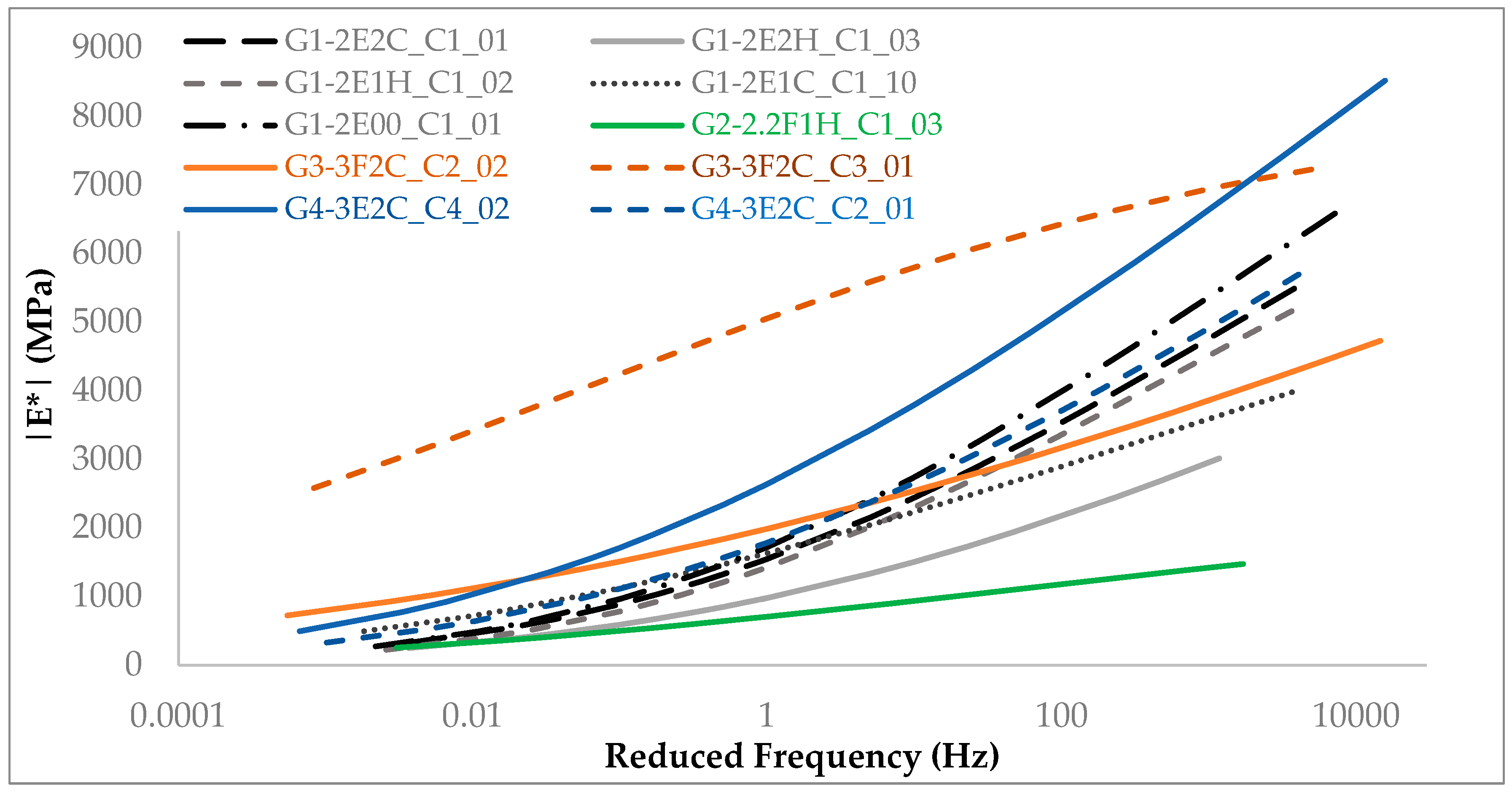
4. Effects of CRAM Composition on |E*| Data

This section covers an investigation into the effects that CRAM’s composition may have on the specimens’ mechanical behavior by means of a dynamic modulus test. The results from this analysis can be beneficial to those interested in cold recycled asphalt mixes and the influence of its mixture composition on viscoelastic properties. In this sense, the Generalized Sigmoidal model was used to fit the test data of CRAMs with different compositions. For better visualization, Figure 9 presents the fit curves for a single specimen replicate (after random selection) of each mixture at a reference temperature of 21.1 °C.

From Figure 8, the effects of the compaction procedure are evident when comparing G3 mixtures compacted with either the modified Proctor compaction (G3-3F2C_C3_01) or the vibratory compaction method (G3-3F2C_C2_02). The modified Proctor method was responsible for a remarkably stiffer mix compared to the specimens compacted using the vibratory method. The same phenomenon was observed with G4 mixtures, where a stiffer behavior due to Proctor compaction (G4-3E2C_C4_02) is observed relative to the specimens prepared with the vibratory compaction (G4-3E2C_C2_01). This phenomenon can be attributed to the lower mixtures’ air void content and the changes in aggregate gradation caused by the impact of the modified Proctor compaction method [36].

Comparing specimens that were compacted by the same procedure (vibratory: G3-3F2C_C2_02 and G4-3E2C_C2_01), there is evidence that foamed stabilized mixtures are less thermo-sensitive than the emulsion stabilized ones. This may be caused by the differences in binder dispersion within the mixture. This is because the foamed asphalt is characterized by dispersing within the mix in a non-continuous manner by creating the so-called “spot welds”. The asphalt emulsion, on the other hand, disperses in a continuous way by creating a thin layer of asphalt binder on the aggregates’ surface [5].

Figure 8 also shows that the dynamic modulus test cannot distinguish the mechanical behavior of the mixtures based on their composition. Analyzing G1 mixtures (gray and black curves), which were compacted and cured using the same methods, it can be concluded that hydrated lime and Portland cement addition caused a stiffness reduction compared to the mixtures without active filler. This reduction was initially unexpected, and it is hypothesized that these results were caused by the absence of confining stress during the |E*| tests, but it needs further investigation. The stiffness difference between G3-3F2C_C2_02 and G2-2.2F1H_C1_03 was expected to occur in the other mixtures as well. Additional mixture characterization and mechanical evaluation might be necessary to properly understand CRAM’s mechanical behavior.

5. Summary and Conclusions

This paper covered the investigation of dynamic modulus |E*| test models and their effects regarding cold recycled asphalt mixtures |E*| data fitting, considering different mixture compositions. The dynamic modulus test database was fitted through different models, after running the linear least-squares method (LSM), and the regressions were analyzed by means of different residuals analysis. Finally, the effects of CRAM composition on |E*| data were graphically assessed. The main conclusions and suggestions of this study are shown below:

• For the specimens evaluated in this study, the Generalized Sigmoidal model and CAM-modified model have been shown to best fit the CRAM’s |E*| test results. Even when the residual analysis has pointed to the selection of another model as the most adequate, both models were still a reliable option for modeling the results without compromising the quality of the regression data. After the analysis of 35 specimens, the Generalized Sigmoidal model was considered the most adequate fit in 51.4% of cases, followed by the Modified CAM model in 31.4% of the cases.
• The Generalized Sigmoidal model and the CAM-modified model were selected as the best models regardless of the aggregate gradations, binder type/content, air void content, RAP content, triaxial resilient modulus (TxRM) values range, active filler type, and curing time. These factors seem to not affect the model selection.
• The residuals graphical analysis of the Generalized Sigmoidal and CAM-modified modeled specimens’ data was satisfactory since it presented a random variation around zero. Therefore, these are acceptable models for fitting CRAM’s |E*| test values.
• The specimen’s compaction method presented a substantial influence on the mechanical behavior of the mixtures. The |E*| test data showed a stiffness increase when high-energy impact methods were used, such as the modified Proctor. This was probably caused by the greater interlocking of the aggregate skeleton, and consequent air void content reduction.
• The |E*| test did not seem to provide a satisfactory evaluation of CRAM specimens when only different mixture compositions were assessed for specimens with the same compaction and curing methods. The absence of confining stresses during the |E*| tests may be the reason for that [7].

References

1. Alkins, A.E.; Lane, B.; Kazmierowski, T. Sustainable Pavements: Environmental, Economic, and Social Benefits of In Situ Pavement Recycling. Transp. Res. Rec. 2008, 2084, 100–103. [Google Scholar] [CrossRef]
2. Halles, F.A.; Thenoux, G.Z. Degree of Influence of Active Fillers on Properties of Recycled Mixes with Foamed Asphalt. Transp. Res. Rec. J. Transp. Res. Board 2009, 2095, 127–135. [Google Scholar] [CrossRef]
3. Jenkins, K. Cracking Behaviour of Bitumen Stabilised Materials (BSMs): Is There Such a Thing? In Proceedings of the 7th RILEM International Conference on Cracking in Pavements, Delft, The Netherlands, 20–22 June 2012; Scarpas, A., Kringos, N., Al-Qadi, I., Loizos, A., Eds.; RILEM Book Series; Springer: Dordrecht, The Netherlands; pp. 1007–1015.
4. Jenkins, K.J.; Collings, D.C. Mix design of bitumen-stabilised materials—South Africa and abroad. Road Mater. Pavement Des. 2017, 18, 331–349. [Google Scholar] [CrossRef]
5. Kuchiishi, A.K.; Antão, C.C.S.; Vasconcelos, K.; Bernucci, L.L.B. Influence of viscoelastic properties of cold recycled asphalt mixtures on pavement response by means of temperature instrumentation. Road Mater. Pavement Des. 2019, 20, S710–S724. [Google Scholar] [CrossRef]
6. Dias, C.R.C.; Núñez, W.P.; Brito, L.A.T.; Johnston, M.G.; Ceratti, J.A.P.; Wagner, L.L.; Fedrigo, W. Bitumen stabilized materials as pavement overlay: Laboratory and field study. Constr. Build. Mater. 2023, 369, 130562. [Google Scholar] [CrossRef]
7. Meneses, J.P.C.; Vasconcelos, K.; Ho, L.L.; Bernucci, L.L.B. Triaxial resilient modulus regression models for cold recycled asphalt mixtures. Road Mater. Pavement Des. 2023, 25 (Suppl. S1), 166–180. [Google Scholar] [CrossRef]
8. Kim, Y.; Lee, H.D.; Heitzman, M. Dynamic Modulus and Repeated Load Tests of Cold In-Place Recycling Mixtures Using Foamed Asphalt. J. Mater. Civ. Eng. 2009, 21, 279–285. [Google Scholar] [CrossRef]
9. Lin, J.; Hong, J.; Xiao, Y. Dynamic characteristics of 100% cold recycled asphalt mixture using asphalt emulsion and cement. J. Clean. Prod. 2017, 156, 337–344. [Google Scholar] [CrossRef]
10. Graziani, A.; Mignini, C.; Bocci, E.; Bocci, M. Complex Modulus Testing and Rheological Modeling of Cold-Recycled Mixtures. J. Test. Eval. 2020, 48, 120–133. [Google Scholar] [CrossRef]
11. Cheng, Z.; Kong, F.; Gao, X. Evaluating dynamic modulus of cold in-place recycling mixture with foamed bitumen using field core samples. Constr. Build. Mater. 2024, 448, 138227. [Google Scholar] [CrossRef]
12. Betti, G.; Airey, G.; Jenkins, K.; Marradi, A.; Tebaldi, G. Active fillers’ effect on in situ performances of foam bitumen recycled mixtures. Road Mater. Pavement Des. 2017, 18, 281–296. [Google Scholar] [CrossRef]
13. Xiao, F.; Yao, S.; Wang, J.; Li, X.; Amirkhanian, S. A literature review on cold recycling technology of asphalt pavement. Constr. Build. Mater. 2018, 180, 579–604. [Google Scholar] [CrossRef]
14. Raschia, S.; Mignini, C.; Graziani, A.; Carter, A.; Perraton, D. Effect of gradation on volumetric and mechanical properties of cold recycled mixtures (CRM). Road Mater. Pavement Des. 2019, 20, S740–S754. [Google Scholar] [CrossRef]
15. Meneses, J.P.C.; Vasconcelos, K.; Bernucci, L.L.B. Stiffness assessment of cold recycled asphalt mixtures—Aspects related to filler type, stress state, viscoelasticity, and suction, Constr. Build. Mater. 2022, 318, 126003. [Google Scholar] [CrossRef]
16. He, Y.; Li, Y.; Zhang, J.; Xiong, K.; Huang, G.; Hu, Q. Performance evolution mechanism and affecting factors of emulsified asphalt cold recycled mixture performance: A state-of art review. Constr. Build. Mater. 2024, 411, 134545. [Google Scholar] [CrossRef]
17. Zhu, C.; Zhang, H.; Li, Q.; Wang, Z.; Jin, D. Influence of different aged RAPs on the long-term performance of emulsified asphalt cold recycled mixture. Constr. Build. Mater. 2025, 458, 139680. [Google Scholar] [CrossRef]
18. T342-11; Standard Method of Test for Determining Dynamic Modulus of Hot Mix Asphalt (HMA). American Association of State Highway and Transportation Officials—AASHTO: Washington, DC, USA, 2011.
19. Vestena, P.M.; Schuster, S.L.; de Almeida, P.O.B., Jr.; Faccin, C.; Specht, L.P.; da Silva Pereira, D. Dynamic modulus master curve construction of asphalt mixtures: Error analysis in different models and field scenarios. Constr. Build. Mater. 2021, 301, 124343. [Google Scholar] [CrossRef]
20. Pellinen, T.; Witczak, M.W.; Bonaqusit, R. Master curve construction using sigmoidal fitting function with non-linear least squares optimization technique. In Proceedings of the 15th ASCE Engineering Mechanics Division Conference, American Society of Civil Engineers, New York, NY, USA, 2–5 June 2002; pp. 82–101. [Google Scholar]
21. Seo, Y.; El-Haggan, O.; King, M.; Lee, S.J.; Kim, Y.R. Air Void Models for the Dynamic Modulus, Fatigue Cracking, and Rutting of Asphalt Concrete. J. Mater. Civ. Eng. 2007, 19, 874–883. [Google Scholar] [CrossRef]
22. Rowe, G.M.; Baumgardner, G.; Sharrock, M.J. A generalized logistic function to describe the master curve stiffness properties of binder mastics and mixtures. In Proceedings of the 45th Petersen Asphalt Research Conference, Laramie, WY, USA, 14–16 July 2008. [Google Scholar]
23. R84-17; Standard Practice for Developing Dynamic Modulus Master Curves for Asphalt Mixtures Using the Asphalt Mixture Performance Tester (AMPT). American Association of State Highway and Transportation Officials—AASHTO: Washington, DC, USA, 2017.
24. Christensen, D.W. Analysis of creep data from indirect tension test on asphalt concrete. J. Assoc. Asph. Paving Technol. 1998, 67, 458–492. [Google Scholar]
25. Zeng, M.; Bahia, H.U.; Zhai, H.; Anderson, M.R.; Turner, P. Rheological modeling of modified asphalt binders and mixtures (with discussion). J. Assoc. Asph. Paving Technol. 2001, 70, 403–441. [Google Scholar]
26. Falchetto, A.C.; Moon, K.H.; Wang, D.; Par, H. A modified rheological model for the dynamic modulus of asphalt mixtures. Can. J. Civ. Eng. 2021, 48, 328–340. [Google Scholar] [CrossRef]
27. Sayegh, G. Variation des Modules de Quelques Bitumes purs et Bétons Bitumineux. Ph.D. Dissertation, Faculté des Sciences de l’université de Paris, Paris, France, 1965. (In French). [Google Scholar]
28. Havriliak, S.; Negami, S. A Complex Plane Analysis of α-Dispersions in some Polymer Systems. J. Polym. Sci. Part C 1966, 14, 99–117. [Google Scholar] [CrossRef]
29. Olard, F.; Di Benedetto, H. General “2S2P1D” model and relation between the linear viscoelastic behaviours of bituminous binders and mixes, Road Mater. Pavement Des. 2003, 4, 185–224. [Google Scholar] [CrossRef]
30. Adam, Y.E. Asphalt Concrete Characterization Using the complex Modulus Technique. Master’s Thesis, Ottawa-Carleton Institute for Civil Engineering, Carleton University, Ottawa, ON, Canada, 2005. [Google Scholar]
31. Biswas, K.G.; Pellinen, T.K. Practical Methodology of Determining the In Situ Dynamic (Complex) Moduli for Engineering Analysis. J. Mater. Civ. Eng. 2007, 19, 508–514. [Google Scholar] [CrossRef]
32. Ping, W.V.; Xiao, Y. A Comparative Study of Laboratory Measured and Predicted Dynamic Modulus for Characterizing Florida Asphalt Mixtures. In Proceedings of the Airfield and Highway Pavements: Efficient Pavements Supporting Transportation’s Future, Bellevue, DC, USA, 15–18 October 2008. [Google Scholar]
33. Kuna, K.; Gottumukkala, B. Viscoelastic characterization of cold recycled bituminous mixtures. Constr. Build. Mater. 2019, 199, 298–306. [Google Scholar] [CrossRef]
34. Behera, A.; Charmot, S.; Asif, A.; Krishnan, J.M. Influence of Confinement Pressure on the Mechanical Response of Emulsified Cold-Recycled Mixtures. J. Mater. Civ. Eng. 2021, 33, 04021297. [Google Scholar] [CrossRef]
35. Kuchiishi, A.K.; Vasconcelos, K.; Bernucci, L.L.B. Effect of mixture composition on the mechanical behavior of cold recycled asphalt mixtures. Int. J. Pavement Eng. 2021, 22, 984–994. [Google Scholar] [CrossRef]
36. Meneses, J.P.C.; Vasconcelos, K.; Bernucci, L.L.B.; Hajj, E. Compaction methods of Cold Recycled Asphalt Mixtures and their effects on pavement analysis. Road Mater. Pavement Des. 2021, 22, S154–S179. [Google Scholar] [CrossRef]
37. Wirtgen GmbH. Cold Recycling—Wirtgen Cold Recycling Technology; Wirtgen GmbH: Windhagen, Germany, 2012. [Google Scholar]
38. Moloto, P.K. Accelerated Curing Protocol for Bitumen Stabilized Materials. Master’s Thesis, Stellenbosch University, Western Cape, South Africa, 2010. [Google Scholar]
39. Kuchiishi, A.K. Mechanical Behavior of Cold Recycled Asphalt Mixtures. Master’s Thesis, Escola Politécnica, Universidade de São Paulo, São Paulo, Brazil, 2019. [Google Scholar]
40. Spiess, A.N.; Neumeyer, N. An evaluation of R2 as an inadequate measure for nonlinear models in pharmacological and biochemical research: A Monte Carlo approach. BMC Pharmacol. 2010, 10, 6. [Google Scholar] [CrossRef]
41. Rawlings, J.O.; Pantula, S.G.; Dickey, D.A. Applied Regression Analysis: A Research Tool; Springer: New York, NY, USA, 1998. [Google Scholar]
42. Akaike, H.A. New Look at the Statistical Model Identification. IEEE Trans. Autom. Control 1974, 19, 716–723. [Google Scholar] [CrossRef]
43. Schwarz, G. Estimating the Dimension of a Model. Ann. Statist. 1978, 6, 461–464. [Google Scholar] [CrossRef]
Figure 1. Flowchart of work organization.
Infrastructures 10 00143 g001
Figure 2. Specimens’ general terminology (as presented in Table 2).
Infrastructures 10 00143 g002
Figure 3. Aggregate gradation curves for (a) asphalt emulsion stabilized mixtures and (b) foamed asphalt stabilized mixtures.
Infrastructures 10 00143 g003
Figure 4. G1-2E1C_C1_01 (a) and G1-2E1C_C1_13 (b) |E*| data modeled through the Generalized Sigmoidal model in the semi-logarithmic space.
Infrastructures 10 00143 g004
Figure 5. G1 mixtures residuals after Generalized Sigmoidal model.
Infrastructures 10 00143 g005
Figure 6. G1 mixtures residuals after Modified CAM model.
Infrastructures 10 00143 g006
Figure 7. G2 (a), G3 (b), and G4 (c) mixtures residuals after the Generalized Sigmoidal model.
Infrastructures 10 00143 g007
Figure 8. G2 (a), G3 (b), and G4 (c) mixtures residuals after the Modified CAM model.
Infrastructures 10 00143 g008
Figure 9. Representative mixtures |E*| master curves on semi-log space using the Generalized Sigmoidal model.
Infrastructures 10 00143 g009