Symmetry-Based Data Augmentation Method for Deep Learning-Based Structural Damage Identification

Abstract

The big data collected from structural health monitoring systems (SHMs), combined with the rapid advances in machine learning (ML), have enabled data-driven methods in practical SHM applications. These methods typically use ML algorithms to identify patterns within features extracted from data representing structural conditions, thereby inferring damage from changes in these patterns. However, data-driven models often struggle to generalize effectively to unseen datasets. This study addresses this challenge through three key contributions: dataset augmentation, an efficient feature representation, and a probabilistic modeling approach. First, a data augmentation method leveraging the symmetric properties of bridge structures is introduced to enhance dataset diversity. Second, a novel damage indicator named Fre-GraRMSC1 is proposed, capable of distinguishing both damage locations and severity. Finally, a probabilistic generative model based on a deep belief network (DBN) is developed to predict damage locations and degrees. The proposed methods are validated using vibration data from a numerical three-span continuous bridge subjected to random vehicle excitations. Results demonstrate high accuracy in damage identification and improved generalization performance.

1. Introduction

Serving as the critical nodes in the transportation infrastructure network, bridges endure harsh environments and suffer performance degradation, posing safety risks. Consequently, structural health monitoring (SHM) emerged in the 1980s as an effective tool for monitoring bridge structures, with damage identification serving as its primary objective [1,2,3,4,5]. Big data of multi-source and multi-type (such as strain, cable force, displacement, acceleration, image, video, etc.) collected from the in-service SHM systems of bridges promotes the development of data-driven methods in SHM. Farrar and Worden note that a standard data-driven method for SHM comprises three key steps [3]: (a) data collection, (b) feature selection and extraction, and (c) model development.

Feature selection and extraction receive the most attention in the literature, with the goal of deriving efficient features from monitoring data capable of distinguishing between undamaged and damaged structural states. The condition-related features, therefore, are also named as damage indicators. Mode parameters are the most common features: features such as DLAC, MDLAC, COMAC, curvature mode method [6], and flexibility matrix approach [7] are proposed for structural damage localization and quantification, further promoting the development and application of vibration-based damage identification methods. Fan et al. [8] comprehensive review of mode parameter-based damage identification methods for beam slab structures prior to 2010, including frequency-based approaches, mode shape-based approaches, curvature mode shape-based approaches, and mixed methods. However, as an overall feature of the structure, frequency is not sensitive to local damage and cannot be used for damage localization. Methods based on mode shapes are severely affected by noise and face problems from incomplete monitoring mode shapes. Nevertheless, as an important structural physical characteristic, the importance of mode parameters cannot be ignored. Hou et al. [9] reviewed the vibration-based damage identification methods for the period 2010–2019 and especially emphasized the inspiration of artificial intelligence and machine learning methods for this field. Besides the mode parameters, damage-specific features and the mined statistical data patterns are also developed and proven to be related to the inherent structural condition of the bridge structure in data-driven methods [10,11,12].

Accompanied by the development of artificial intelligence in the field of civil engineering, deep learning (DL) models [13,14,15] are frequently employed in step (c) model development in the data-driven SHM method in the recent decade. With the mechanism of end-to-end training, implicit damage-related features are automatically learned in the training process in DL models. Most of the DL-based applications are in the supervised learning framework due to the easy convergence in modeling the complex correlations in the dataset. These approaches rely on training the network with abundant high-quality datasets with supervised damaged labels, such as damage locations and damage degrees. For example, Ding et al. [16] built a deep belief network (DBN) with an arctan-based sparse constraint for structural damage identification, which utilized vibration characteristics as network input and damage information as network output. Results indicated that the proposed method had obtained accurate and stable damage identification results even under uncertain and limited data. Wang et al. [17] developed a deep residual network for damage identification which learns damage features from vibration data and maps to the damage index labels. The feasibility and accuracy of the method are evaluated in both numerical and experimental studies. The developed network retains both low- and high-level features and simultaneously enhances feature learning and transmission capabilities, therefore achieving high accuracy and effectiveness for damage identification in numerical studies considering both modeling uncertainties and measurement noises.

In essence, DL and ML models establish a nonlinear fitting function that maps from the input features to the output damage labels, which leads to the generalization problem when extrapolation in the unseen new dataset [18]. It is worth mentioning that the generalization issue due to the dataset limitation widely exists in all fields in the practical DL applications, not only in the SHM field. Because of the model complexity of the DL model, this generalization usually exhibits as an overfitting problem. Therefore, dataset diversity, i.e., abundant datasets obtained from various damage cases, is essential to train a well-performed and well-generated DL model. However, the labels and rich damage combinations can be very expensive to obtain from the SHM system of a real-world structure; thus, the real dataset are usually incomplete and long-tailed. The long tail effect (long-tailed class distribution) means that in the dataset, a small subset of classes (head classes) contains many sample points while the other classes (tail classes) have only a few samples [19]. This class imbalance phenomenon leads to excellent performance of the DL model in the head classes but inefficiency in the tail classes, resulting in a significant decrease in overall accuracy. Additionally, the “black-box” issue of the DL models exacerbates this generalization issue because the automatically extracted features in the end-to-end learning framework are implicitly related to the structural condition.

DL community efforts in two ways: the model selection [20] and data augmentation [21,22]. Model selection relies on prior knowledge, such as the regularization, domain-specific constraints, physics-informed mechanisms, and exploitability of the DL model. Data augmentation refers to the value of generating equivalent data from limited samples without substantially increasing the amount of data. In other words, data augmentation involves making minor modifications to existing data or synthesizing new data from the existing dataset to increase the quantity of data. For example, classic data augmentation techniques applied in computer vision involve generating more diverse samples by manipulating input data (images/videos) through geometric transformations and photometric transformations. However, such approaches are not applicable to the vast majority of problems in damage identification tasks since the variety of damage cases remains underrepresented. In recent years, explainable ML approaches, transfer learning algorithms, and physics-informed approaches have been proposed to alleviate the generalization ability and insufficient capacity problem in the DL community. Among them, physics-informed neural networks (PINNs) are developed to combine physics prior knowledge and data [23,24]. Physics-inspired data augmentation methods can be integrated with them, which generate diverse training data to enhance network training and improve generalization ability through incorporating structural physical properties into data augmentation methods. In SHM, instead of purely data-driven methods, data-driven methods that combine the physical information of the mode-based indicators are supposed to improve the generalization ability of structural damage identification. However, the SHM community has not seen many such successes.

DL-based methods for structural damage identification in SHM also faced these challenges. Fernandez et al. [25] developed a hybrid supervised DL approach for damage identification using bridge structures, Fathnejat et al. [26] proposed a convolutional-attention-recurrent neural architecture and investigated the damage identification under temperature variation, Bao et al. [27] proposed a transfer learning network for the structural condition identification with limited training data, Huang et al. [28] introduced noises to augment the training data and proposed a data augmentation-adaptive CNN for structural damage identification of a 3-span bridge structure. However, current data augmentation approaches in SHM remain largely limited to noise injection and rarely utilize inherent physical information.

In summary, the insufficiency and incompleteness of labeled datasets in DL-based methods present significant generalization challenges for damage identification in SHM. To address this limitation, we propose three targeted approaches aligned with the established data-driven SHM framework. In the data collection step, a symmetry-based data augmentation method based on the symmetry of the structure is proposed to increase the richness and diversity of the dataset. In the feature selection and extraction step, we develop a domain-specific damage indicator as the input feature instead of training an end-to-end feature by the DL model. The new damage indicator named Fre-GraRMSC1, derived from mode parameters, is proven to be more robust and efficient than existing mode-based indicators. In the model development step, we frame the damage identification problem as a generation problem by the input features and introduce DBN as the probabilistic generative model.

The proposed approaches are validated using vibration data from a numerical three-span continuous beam bridge released at the 3rd International Conference on Structural Health Monitoring (IC-SHM). Results demonstrate enhanced accuracy and improved generalization capabilities for the DL-based framework.

This paper is organized as follows. In the Methodolgy section, we present the data-augmentation methods, damage indicator, and the DBN model employed in this paper. In Case Studies, we describe the open-source dataset released during the competition, the pre-processing of the dataset, the implementation details of the proposed approaches, and the analysis of the results. Finally, in the Conclusion section, we summarize the main findings of this paper.

2. Methodology

The proposed methodology addresses generalization challenges in three key aspects: (1) data augmentation, (2) domain-specific feature engineering, and (3) probabilistic generative modeling. These align directly with the three fundamental steps of data-driven SHM frameworks.

2.1. Data-Augmentation

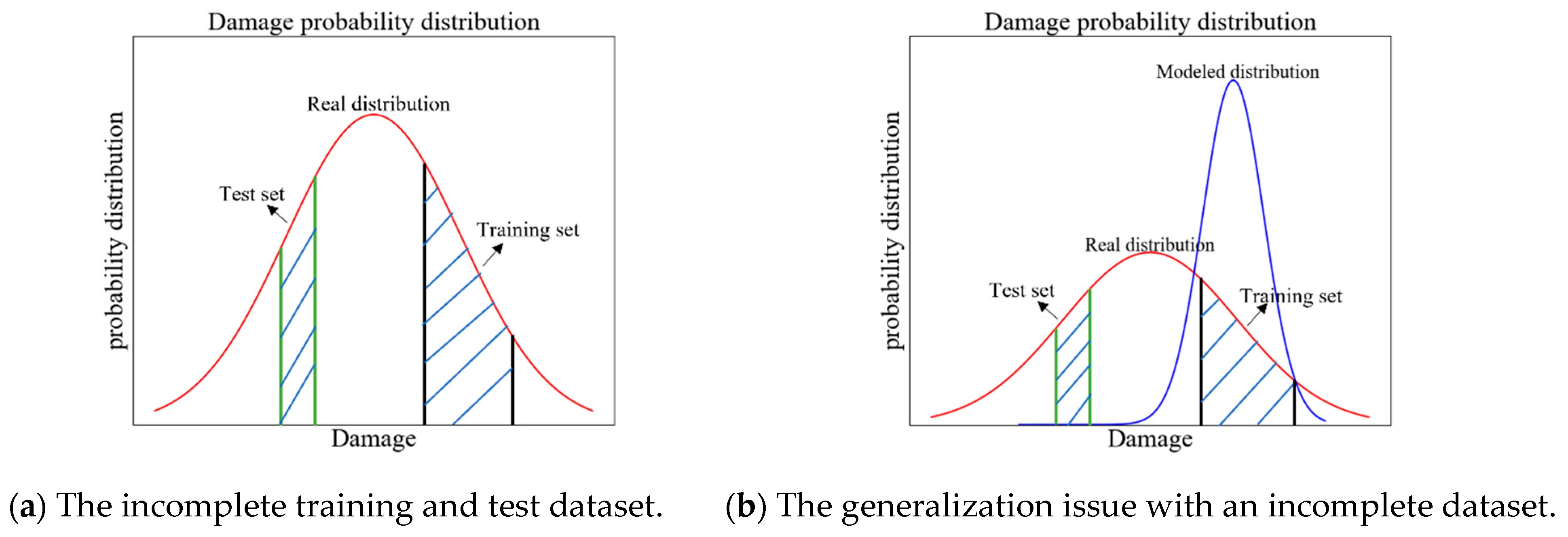
Insufficient, incomplete, and long-tailed datasets undermine the generalization capability of data-driven damage identification methods on test sets. This limitation stems from violations of the independent and identically distributed (i.i.d.) assumption fundamental to ML/DL algorithms, where training and test data are presumed to share identical underlying distributions.

Let $p_{damage}$ denotes the probability distribution encompassing all possible damage cases (varying in location and severity). Under ideal conditions, both the training and test datasets are randomly sampled from $p_{damage}$, satisfying the i.i.d. assumption [29]. In this case, DL models generalize reliably. However, the training and test datasets sampled from the limited datasets with few damage cases may diverge significantly, as illustrated in Figure 1. Consequently, models trained on $p_{train}$ fail to generalize to $p_{test}$’s distribution, as illustrated in Figure 1. This distribution shift constitutes a fundamental challenge when deploying DL models in real-world SHM applications.

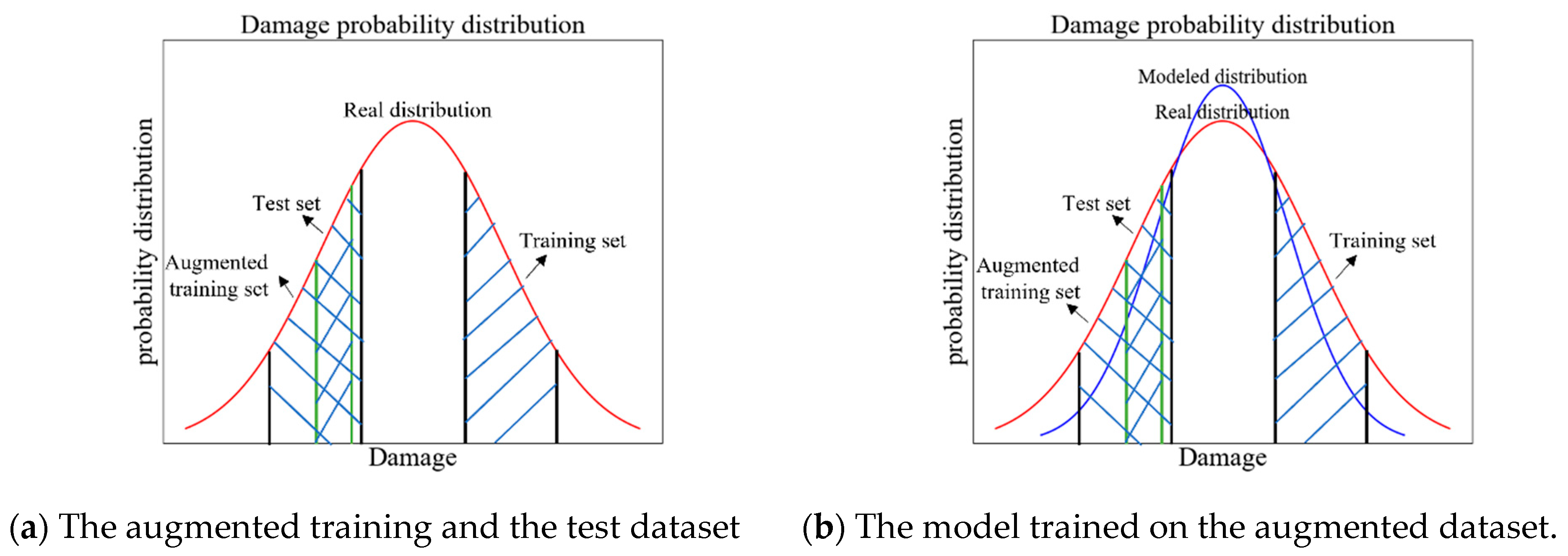
Data augmentation aims to increase the diversity of training data and forms an integral component of a broad set of regularization techniques that are used to improve data-driven models. Compared with the classical data augmentation approaches by transformation and deformation of the images, this section proposes a physics-inspired data augmentation method that incorporate physical information to increase the diversity of the training dataset. One of the most important inherent physical properties of the bridge structures is symmetry. For example, the mode shapes are in symmetric modes and asymmetric modes for the symmetric bridge structure. Therefore, we can add the “physical-symmetric” data and augment the distribution of the training dataset to approximate the real distribution, as illustrated in Figure 2a. The trained DL-based damage identification model thus will generalize better, as illustrated in Figure 2b.

2.2. Damage Sensitive Feature

Considering the motion differential equations for an N-degree-of-freedom (DOF) linear time-invariant structure:

$$M\ddot{x}\left(t\right)+C\dot{x}\left(t\right)+Kx\left(t\right)=f\left(t\right)$$

(1)

where $M$, $C$, and $K$ denote the mass matrix, damping matrix, and stiffness matrix, respectively, $x\left(t\right)$ denotes the structural displacement vector, and $f\left(t\right)$ denotes the load vector. The structural state equation can be expressed by Equations (2) and (3).

$$X\left(t\right)=\left[\begin{array}{c}\dot{x}\left(t\right)\\ x\left(t\right)\end{array}\right]$$

(2)

$$\begin{gathered} X\left(k+1\right)=AX\left(k\right)+BF\left(k\right) \\ Y\left(k\right)=CX\left(k\right) \end{gathered}$$

(3)

where $A$ denotes the structural system matrix, $B$ denotes the load action position matrix, $C$ denotes the structure monitoring position matrix, $X\left(k\right)$ denotes the structural state vector at time $k∆$, $Y\left(k\right)$ denotes the monitoring structural response vector at time $k∆$, $F\left(k\right)$ denotes the input vector at time $k∆$, $k$ and $∆$ are the sampling points and interval, respectively.

Mode parameters, including mode shapes and natural frequencies, can be identified with Equations (4)–(6):

$${\mathsf{\Phi }}^{-1}A\mathsf{\Phi }=Z$$

(4)

$$\begin{array}{l}{\mathsf{\omega }}_i=\sqrt{\left({\lambda }_i^R\right)+\left({\lambda }_i^I\right)}\\ {\lambda }_i={\lambda }_i^R+i{\lambda }_i^I={\displaystyle \frac{1}{∆t}}\ln (z_i) \end{array}$$

(5)

$$\widehat{\mathsf{\Phi }}=C\mathsf{\Phi }$$

(6)

where $\mathsf{\Phi }$ denotes the eigenvector matrix, $Z=\left[z_1,z_2,\cdots ,z_{2N}\right]$ is the eigenvalue matrix. ${\mathsf{\omega }}_i$ is the i-th nature frequency, ${\lambda }_i$ is the eigenvalue of the continuous state equations, ${\lambda }_i^R$ and ${\lambda }_i^I$ denotes the real and imaginary parts of ${\lambda }_i$, $\widehat{\mathsf{\Phi }}$ denotes the identified mode shapes (mode shapes at the sensor placement position). In Section 3, NExT-ERA method [30,31] is employed.

(1)

The Fre-GraRMSC1 Indicator

Damage-induced alterations to mass/stiffness properties consequently manifest as changes in model parameters. Crucially, mode shapes exhibit the most sensitive feature to indicate damage location, whereas natural frequencies show greater sensitivity to damage severity than location [8]. Despite the established insensitivity of natural frequencies and naturally excited low-order mode shapes to localized damage, they remain critical structural attributes. Through careful feature engineering, derived indicators based on these parameters can still contribute significantly to damage identification. Leveraging this prior knowledge of structural dynamics, this paper proposes Fre-GraRMSC1, a physics-informed damage indicator derived from first-order mode shape and natural frequencies.

The 1st first order mode shape change (RMSC1) defined in Equation (7) is employed to enhance the sensitivity,

$$RMSC1={\displaystyle \frac{{{\phi }_1}^d-{{\phi }_1}^u}{{{\phi }_1}^u}}$$

(7)

Furtherly, the gradient of RMSC1 (GraRMSC1) is developed, as illustrated in Equation (8).

$$\begin{gathered} {Grad}_{i,j}=({RMSC1}_i-{RMSC1}_j)/d_{ij} \\ GraRMSC1=[{Grad}_{1,2},{Grad}_{2,3},\cdots ,{Grad}_{i,j}\cdots {Grad}_{n-1,n}] \end{gathered}$$

(8)

where ${{\phi }_1}^u$, ${{\phi }_1}^d$ represents the 1st-order mode shapes before and after damage, respectively. $n$ is the number of DOF, ${RMSC1}_i$ and ${RMSC1}_j$ are the 1st order mode shape change (RMSC1) at the i-th and j-th degree of freedom, $d_{ij}$ is the distance between the i-th and j-th degrees of freedom on the structure.

While the gradient-based GraRMSC1 preserves relative spatial trends in mode shapes, the gradient operation inherently eliminates absolute amplitude information critical for quantifying damage severity across measurement points. To incorporate damage severity, the 1st-order frequency change rate $\Delta {\omega }_1$ before and after damage is introduced, as illustrated in Equation (9).

$$\Delta {\omega }_1={\displaystyle \frac{{{\omega }_1}^t-{{\omega }_1}^i}{{{\omega }_1}^i}}$$

(9)

where ${{\omega }_1}^t,{{\omega }_1}^i$ denotes the 1st-order frequency of the initial and the test cases.

The integration of GraRMSC1 and $\Delta {\omega }_1$ forms the Fre-GraRMSC1 damage indicator. This hybrid feature serves as physics-informed input to neural network models, explicitly incorporating structural mechanics to address generalization limitations. Crucially, Fre-GraRMSC1 simultaneously resolves two fundamental challenges in structural damage identification, i.e., localization sensitivity and damage level property. By fusing physics-derived features with data-driven learning, this approach enhances both robustness against distribution shifts and model interpretability.

2.3. Deep Belief Network Model

A deep belief network (DBN) is introduced as the inference model to generate the conditional probability of damage given the observed SHM data. Unlike deterministic deep learning approaches, this probabilistic formulation learns a comprehensive joint distribution of input data, enabling robust damage identification under uncertainty. The DBN is composed of multiple layers of restricted Boltzmann machines (RBMs) has also been proven to succeed in specific domains [32,33,34].

(2)

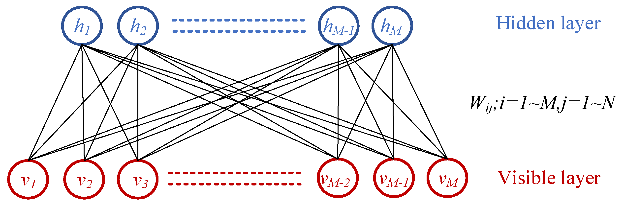
Restricted Boltzmann Machine

A restricted Boltzmann machine (RBM) is a generative stochastic model with two fully connected, undirected layers: a visible layer and a hidden layer (Figure 3). It models probability distributions of input data through interactions between these layers. The inputs of the visible layer are represented by the visible vector v = (v₁, v₂, v₃, ⋯ v_i, ⋯)^T, and the bias vector is b = (b₁, b₂, b₃, ⋯ b_i, ⋯)^T. Units in the subsequent hidden layer are represented by the hidden vector h = (h₁, h₂, h₃, ⋯ h_j, ⋯)^T, and the bias vector in the hidden layer is c = (c₁, c₂, c₃, ⋯ c_i, ⋯)^T. Units are binary-valued, i.e., v_i ∈ {0,1}, h_j ∈ {0,1}; and are conditionally independent within each layer. $\left(\mathit{h},\mathit{v}\right)$ is thus the state of the RBM. W = (w_ij) are weights that connect the interlayer visible units v and the hidden units h.

The RBM’s energy function $\mathit{E}$ and the joint probability distribution is given by:

$$\mathit{E}\left(\mathit{h},\mathit{v}\right)=-\left({\mathit{b}}^{\mathit{T}}\mathit{v}+{\mathit{c}}^{\mathit{T}}\mathit{v}+{\mathit{v}}^{\mathit{T}}\mathit{W}\mathit{h}\right)=-\sum _{i\in \mathrm{visible}}{b}_i{v}_i-\sum _{i\in \mathrm{hidden}}{c}_i{h}_i-\sum _{i,j}{v}_i{h}_j{\omega }_{ij}$$

(10)

$$p(\mathit{h},\mathit{v})={\displaystyle \frac{1}{Z}}{e}^{-E(\mathit{h},\mathit{v})}, \mathit{Z}={\sum }_{\mathit{v}}{\sum }_{\mathit{h}}{e}^{-E(\mathit{h},\mathit{v})}$$

(11)

where $\mathit{Z}$ represents the partition function. Therefore, the corresponding probability $p(\mathit{h},\mathit{v})$ decreases when the value of the energy function increases and increases vice versa. The marginal probability given visible vector v or hidden vector h are:

$$p\left(\mathit{v}\right)={\displaystyle \frac{1}{Z}}{\sum }_{\mathit{h}}{e}^{-E\left(\mathit{v},\mathit{h}\right)}={\displaystyle \frac{{\sum }_{\mathit{h}}{e}^{-E\left(\mathit{v},\mathit{h}\right)}}{{\sum }_{\mathit{v}}{\sum }_{\mathit{h}}{e}^{-E\left(\mathit{v},\mathit{h}\right)}}}, p\left(\mathit{h}\right)={\displaystyle \frac{1}{Z}}{\sum }_{\mathit{v}}{e}^{-E\left(\mathit{v},\mathit{h}\right)}={\displaystyle \frac{{\sum }_v{e}^{-E\left(\mathit{v},\mathit{h}\right)}}{{\sum }_{\mathit{v}}{\sum }_{\mathit{h}}{e}^{-E\left(\mathit{v},\mathit{h}\right)}}}$$

(12)

As the connection only exists between units in different layers, given visible vector v or hidden vector h, the hidden vector h and visible vector v are all conditionally independent. The conditional probability is thus obtained:

$$p\left(h_j=1|\mathit{v}\right)={\displaystyle \frac{1}{1+\mathit{exp}[-(c_j+{\sum }_i{v}_i{W}_{ij})]}}=\sigma \left(c_j+\sum _i{v}_i{W}_{ij}\right)$$

(13)

$$p\left(v_i=1|\mathit{h}\right)={\displaystyle \frac{1}{1+\mathit{exp}[-(b_i+{\sum }_j{h}_j{W}_{ij})]}}=\sigma \left(b_i+\sum _j{h}_j{W}_{ij}\right)$$

(14)

where $\sigma \left(x\right)={\displaystyle \frac{1}{1+e^{-x}}}$ is the sigmoid activation function. Thus, the RBM module can be expressed in a parameterized form.

Parameters W, b, and c can be learned by maximizing the likelihood function in Equation (16):

$${\displaystyle \frac{\partial p\left(\mathit{v}|\mathit{h}\right)}{\partial \mathit{\theta }}}=-{\sum }_{\mathit{h}}p\left(\mathit{h}|\mathit{v}\right){\displaystyle \frac{\partial E\left(\mathit{h},\mathit{v}\right)}{\partial \mathit{\theta }}}+{\sum }_{\mathit{v},\mathit{h}}p\left(\mathit{v}|\mathit{h}\right){\displaystyle \frac{\partial E\left(\mathit{h},\mathit{v}\right)}{\partial \mathit{\theta }}}$$

(15)

where $\mathit{\theta }=[\mathit{w},\mathit{b},\mathit{h}]$ represent the parameter set.

CD-k algorithm [28,29] is introduced to train the parameters, where k is the number of contrast information, and k = 1 is employed by Hinton’s experience [35,36]. The pseudo-code is listed as Algorithm 1.

Algorithm 1: CD-k algorithm

Input: visible vector v Output: hidden vector h Procedures: Step 1: Randomly select a sample from the training input dataset as the visual layer input vi. Step 2: Calculate the conditional probability $p(h_j=1|\mathit{v})$ for each hidden unit hj in the hidden layer according to Equation (13) to complete the forward updating from the visual layer to the hidden layer. Step 3: Calculate the conditional probability $p(v\prime =1|\mathit{h})$ for each visual unit $v_i$ in the visual layer according to Equation (14) to complete the reverse updating from the hidden layer to the visual layer. Step 4: Calculate the conditional probability $p(h_j\prime =1|\mathit{v}\prime )$ again according to Equation (13). Step 5: Iterate steps (2–4) for k times.

With $p(h_j=1|v)$ and $p(h_j\prime =1|v\prime )$, parameters are learned using the momentum method, as follows:

$$w_{ij}\leftarrow \alpha w_{ij}+\eta \left[v_{i}p\left(h_j=1|v\right)-v_{i}p\left(h_j\prime =1|v\prime \right)\right]$$

(16)

$$b_i\leftarrow \alpha b_i+\eta \left(v_i-v_i\prime \right)$$

(17)

$$c_j\leftarrow \alpha c_j+\eta \left[p\left(h_j=1|v\right)-p\left(h_j\prime =1|v\prime \right)\right]$$

(18)

where $\alpha$ is momentum, $\eta$ is the learning rate, $v_i\prime$ and $h_j\prime$ represent the updated visible and hidden units, respectively.

(3)

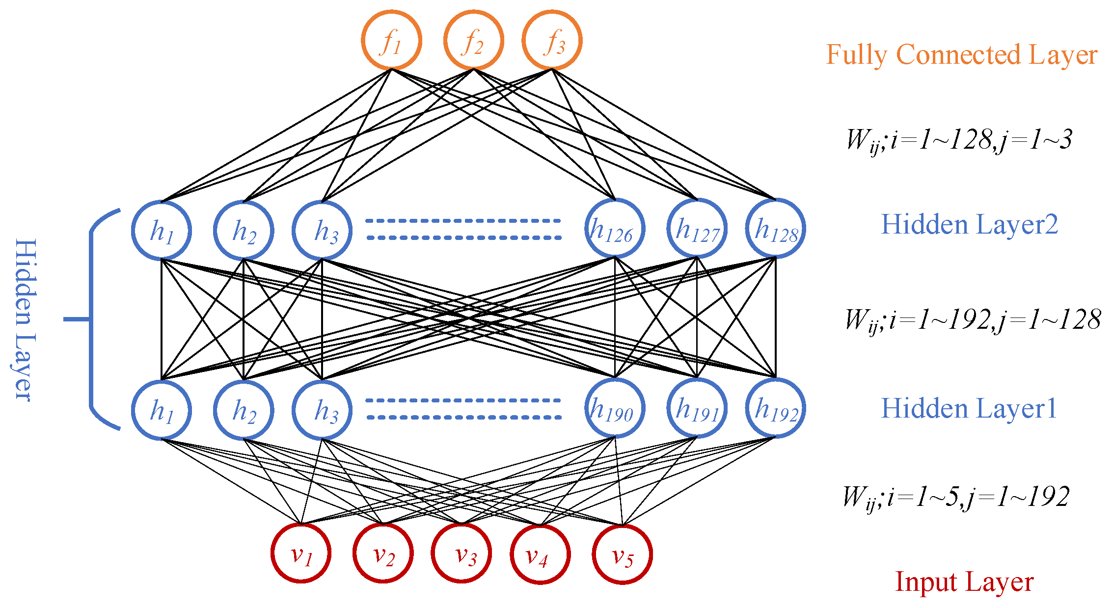
DBN model

DBN model stacks several RBMs with a fully connected layer serving as an output layer, as illustrated in Figure 4. Unlike the conventional feedforward network probabilistic model that predicts the probability $p\left(h\right|v)$ only, DBN is treated as a probabilistic generative graph model that infers the probabilities $p\left(v\right|h)$ and $p\left(h\right|v)$ simultaneously.

The training process of DBN involves two stages: layer-wise pretraining and fine-tuning. In the layer-wise pretraining stage: a. the first RBM processes the input (Fre-GraRMSC1 damage indicators), b. visible units accept continuous values (non-binary inputs permitted), c. updated via contrastive divergence (CD-k) algorithm, d. hidden layer outputs become visible inputs for the next RBM, e., the process repeats greedily for the subsequent RBMs. In the fine-tuning stage, information is propagated bottom-up to the last FCN-output layer, and all the parameters are further updated through supervised learning using a gradient descent algorithm.

The overall workflow of the proposed method is summarized as follows:

(1)

Data acquisition

(1.1)

Simulation/monitoring.

(1.2)

symmetry-based augmentation.

(2)

Pre-process

(2.1)

Temporal segmentation.

(2.2)

Feature extraction: Fre-GraRMSC1.

(3)

DBN model training

(3.1)

Pretrain the RBM via CD-k algorithm.

(3.2)

Fine-tune via BP algorithm.

(3.3)

K-fold cross-validation.

(4)

Damage Identification

Outputs damage location and severity level using the trained DBN model.

3. Case Studies

3.1. The Simulation Dataset

As data augmentation is the most highlighted step in the proposed approach, four cases are designed to validate the effectiveness and robustness when considering augmentation under the same damage indicator and DBN model. Case I considers the condition of perfect symmetry without data augmentations in the training dataset, i.e., 11 element damage simulations are used to form the training dataset. Case II considers the perfect symmetry case with data augmentations in the training dataset, i.e., the training dataset consists of 11 calculated damage simulations and 10 augmented simulations. Case III and IV consider the im-perfect symmetry case with augmentations in the training dataset. The imperfect symmetry in Case III and IV are simulated by the introduced random noises in the stiffness of each element with the amplitude of 3% and 5%, respectively. Nowadays sensors, such as accelerometers and especially CV-based measurements [37], 5% is an acceptable noise level in real application. The imperfect symmetry in Case III and IV are simulated by the introduced random noises in the stiffness of each element with the amplitude of 3% and 5%. Therefore, the comparative analysis between Case I and II shows the effectiveness of the physical-based augmentation, and the comparative analysis between Case II, III, and IV illustrates the robustness under the imperfect symmetry assumption.

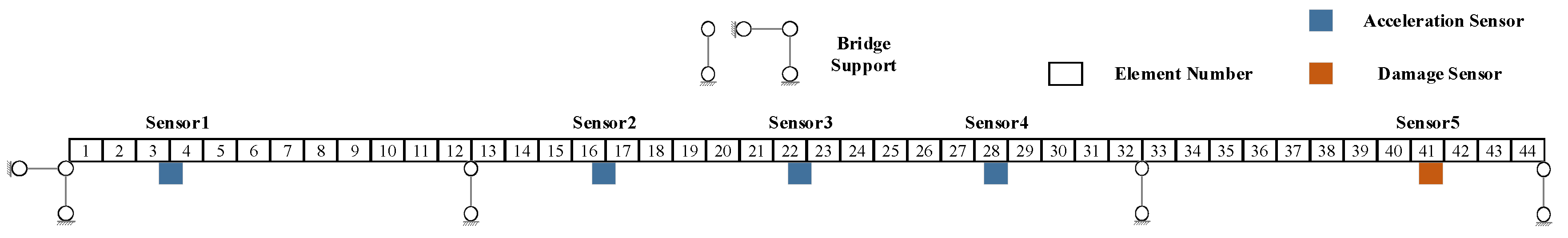
All simulation cases are based on the three-span continuous beam bridge model released on Project 3 of the IC-SHM 2022, as illustrated in Figure 5. The bridge is divided into 44 elements, and the length of each element is 0.5 m. Accelerometers A1-A5 are arranged on the bridge from left to right to obtain the vertical acceleration under random vehicle excitation developed and used in [38,39,40]. Elements No. 7, 22, and 38 are set to be the elements with potential damage, and the damage is simulated by the decrease in stiffness of the target elements. Three Percent level noises are also added to the simulation accelerations to verify the robustness of the proposed method. The simulation dataset is illustrated in

Table 1. Simulation dataset for all Cases.

Serial Number		First Frequency (Hz)				Damage Condition
		Case I	Case II	Case III	Case IV	Ele 7	Ele 22	Ele 38
No damage	1	9.4367	9.4367	9.4252	9.8599	0%	0%	0%
Training dataset: Damaged	2	9.3613	9.3613	9.3542	9.7811	0%	20%	0%
	3	9.3093	9.3093	9.3050	9.7268	0%	30%	0%
	4	9.2421	9.2421	9.2415	9.6565	0%	40%	0%
	5	9.4251	9.4251	9.4138	9.8477	10%	0%	0%
	6	9.3924	9.3924	9.3814	9.8135	30%	0%	0%
	7	9.3345	9.3345	9.3243	9.7530	50%	0%	0%
	8	9.3356	9.3356	9.3288	9.7542	20%	20%	0%
	9	9.2167	9.2167	9.2164	9.6300	20%	40%	0%
	10	9.2933	9.2933	9.2870	9.7100	40%	20%	0%
	11	9.1751	9.1751	9.1752	9.5864	40%	40%	0%
Test dataset Damaged	12	9.4028	9.4028	9.3933	9.8245	0%	10%	0%
	13	9.1520	9.1520	9.1561	9.5624	0%	50%	0%
	14	9.4107	9.4107	9.3996	9.8327	20%	0%	0%
	15	9.3680	9.3680	9.3575	9.7881	40%	0%	0%
	16	9.3101	9.3101	9.3035	9.7276	20%	20%	20%
	17	9.1099	9.1099	9.1106	9.5184	40%	40%	40%

Note: Case I—perfect symmetry, no augmentation; Case II—perfect symmetry, augmentation; Case III—3% uncertainty in all elements’ stiffness, augmentation; Case IV—5% uncertainty in all elements’ stiffness, augmentation.

. Simulations No. 2–11 are used in the training dataset, and 12–17 are used in the test dataset. It is noted that in order to investigate the generalization ability to the unseen new data, damage in Element No. 38 is not included in the training dataset for all these cases while it is contained in the test dataset. Simulations No. 12 and 13 are designed to investigate the extrapolation ability of the proposed approach.

3.2. Data Pre-Processing

Three steps are contained in the data pre-processing procedure: data augmentation, time series segmentation, and feature extraction. The simulated dataset for Case II is employed as the demonstration example in the following section.

(1)

Symmetry-based Data Augmentation

Physical law can usually help a lot with the generalization ability of a data-driven model by posing prior knowledge and constraints. For the three-span continuous bridge structure, a simple physical law is the symmetry properties as mentioned above:

• Structural symmetry: The bridge structure has 44 elements, and the placement of constraints and the division of mass and stiffness are all symmetric. Therefore, it is a bridge structure with a perfectly symmetrical architectural design.
• Sensor symmetry: Sensors A1-A5 are symmetrically allocated on the investigated bridge.
• Damage symmetry: Elements No. 7 and 38 are symmetrical about No. 22 and the symmetry axis, i.e., three potentially damaged elements are symmetric.

Based on the above symmetry properties and the loading condition, combined the data augmentation method proposed earlier, damage elements on No. 7 or 38 can be extrapolated to No. 38 or 7, which is symmetrically situated along the bridge’s axis. The structural response for damage at No. 7 or 38 can be considered equivalent to that when equally severe damage occurs at its symmetric position: No. 38 or 7. Therefore, the sensor serial number of each training set can be flipped symmetrically (i.e., the original A1-A5 sensor becomes A5-A1 sensor), and the damage conditions is flipped symmetrically (the original damage of No. 7, 22, and 38 becomes damage of No. 38, 22, and 7) in the same way. Thus, the additional training sets 18–27 can be obtained based on the flipped training sets 1–11 and form a total of 20 damage cases, as shown in

Table 2. The augmented training dataset for Cases I, II, and III.

Serial Number		First Frequency (Hz)				Damages
		Case I	Case II	Case III	Case IV	Ele 7	Ele 22	Ele 38
No damage	1	9.4367	9.4367	9.4252	9.8599	0%	0%	0%
Original	2	9.3613	9.3613	9.3542	9.7811	0%	20%	0%
	3	9.3093	9.3093	9.3050	9.7268	0%	30%	0%
	4	9.2421	9.2421	9.2415	9.6565	0%	40%	0%
	5	9.4251	9.4251	9.4138	9.8477	10%	0%	0%
	6	9.3924	9.3924	9.3814	9.8135	30%	0%	0%
	7	9.3345	9.3345	9.3243	9.7530	50%	0%	0%
	8	9.3356	9.3356	9.3288	9.7542	20%	20%	0%
	9	9.2167	9.2167	9.2164	9.6300	20%	40%	0%
	10	9.2933	9.2933	9.2870	9.7100	40%	20%	0%
	11	9.1751	9.1751	9.1752	9.5864	40%	40%	0%
Augmented	18		9.3613	9.3542	9.7811	0%	20%	0%
	19		9.3093	9.3050	9.7268	0%	30%	0%
	20		9.2421	9.2415	9.6565	0%	40%	0%
	21		9.4251	9.4138	9.8477	0%	0%	10%
	22		9.3924	9.3814	9.8135	0%	0%	30%
	23		9.3345	9.3243	9.7530	0%	0%	50%
	24		9.3356	9.3288	9.7542	0%	20%	20%
	25		9.2167	9.2164	9.6300	0%	40%	20%
	26		9.2933	9.2870	9.7100	0%	20%	40%
	27		9.1751	9.1752	9.5864	0%	40%	40%

Notes: blue labeled is the original dataset without data augmentation, and the red labeled is the dataset with augmentation. No augmentations are employed in Case I.

. Together with the undamaged case, we finally obtain 21 damage cases in the training dataset (except for Case I, without any augmentations) and 6 cases in the test dataset.

(2)

Time series segmentation

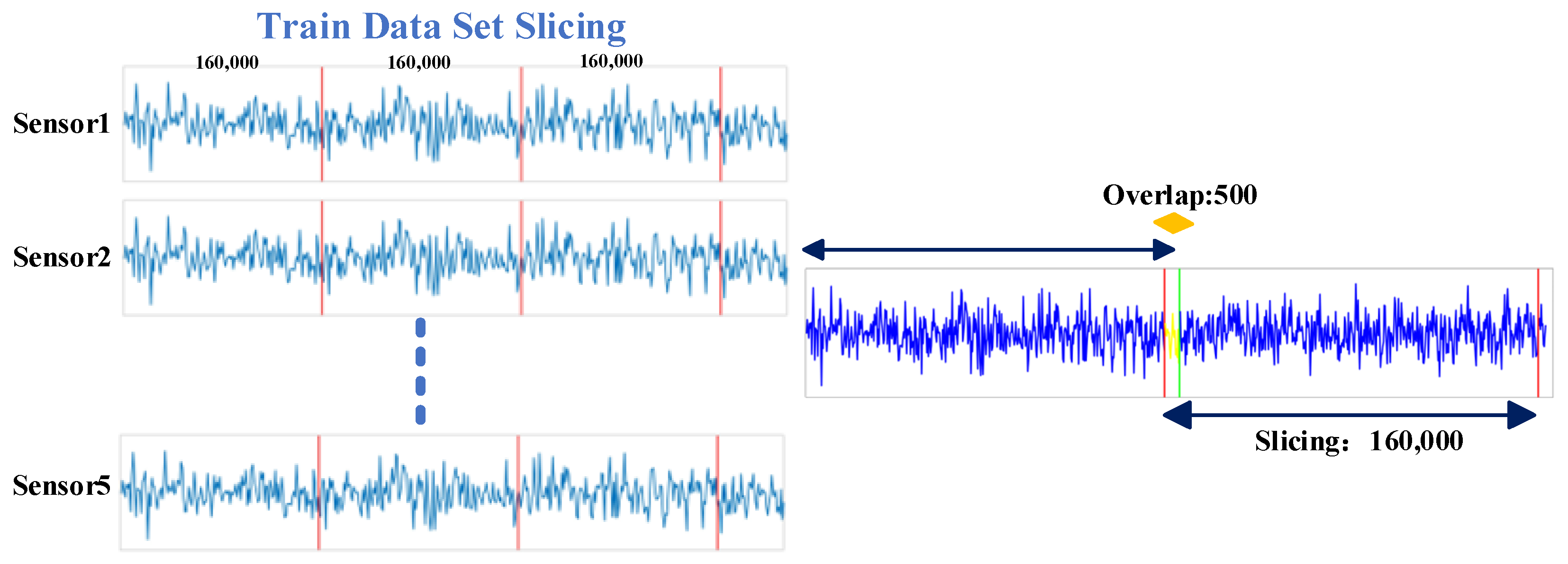
Data segmentation of the monitoring data $\mathit{X}={\left\{{\mathit{x}}_1,{\cdots ,\mathit{x}}_i, \cdots ,{\mathit{x}}_n\right\}}^T$ is then conducted. Where X denotes the augmented dataset of the monitoring accelerations, ${\mathit{x}}_i={[x_{i1},{\cdots ,x}_{it},{\cdots ,x}_{iT}]}^T$ denotes the monitored time series of the i-th accelerometer, n = 5 denotes the total number of accelerometers, and T is the total length of the time series. Therefore, the shape of the monitoring acceleration obtained from the five accelerometers in one damage condition is 5 × 200,000, which refers to the depth (number of accelerometers) and length of the data, respectively. The shape of the whole dataset is 21 × 5 × 200,000, where 21 corresponds to the number of damaged cases in Table 2 and the undamaged case. Small segmentations of the whole dataset are sliced for efficient training. The dataset is sliced into pieces with a length of 160,000 and 500 overlapping between two adjacent pieces, as illustrated in Figure 6. The train dataset of 1620 × 5 × 160,000 is finally obtained.

(3)

Feature Extraction

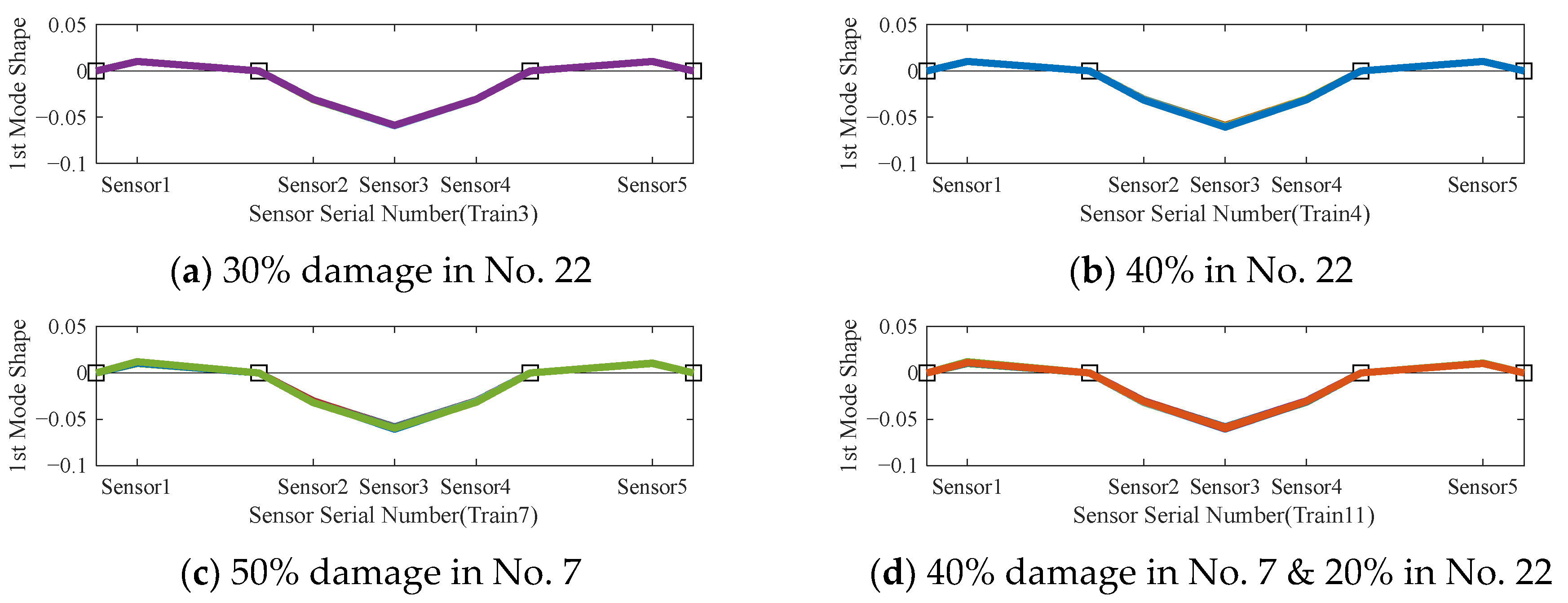
The 1st-order mode shape and 1st-order frequency of the bridge structure are initially identified with the NExT-ERA method, as illustrated in Figure 7. Figure 7a–d depicts the identified mode shapes based on monitoring data under four different damage cases, which correspond to damages in training sets. Different colors in each figure represent different samples of the pieces the results identified through different data slices. The mode shapes shown in Figure 7a–d under different damage cases are similar, indicating insufficient sensitivity to the occurrence of damage.

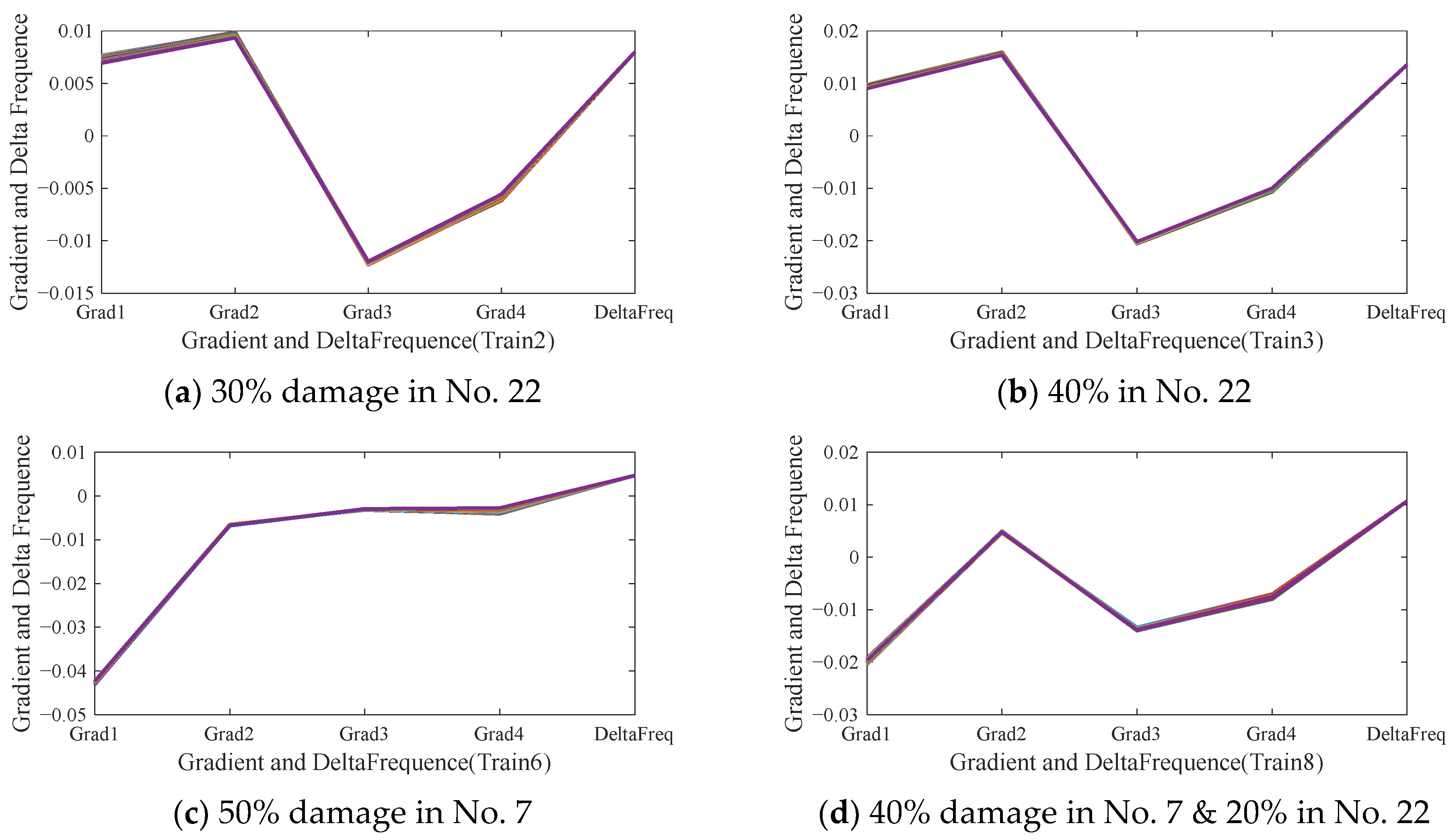
RMSC1 obtained of the same samples from training set 2, 3, 6, and 8 in Table 1 are shown in Figure 8a–d. The RMSC1 curves in Figure 8a,b exhibit noticeable differences between the two damage cases with 20% and 30% damage degree in the same element NO.22. Furthermore, Figure 8b,c differentiate the damage locations from train 2 and train 6 with the same damage degree of 30%, the corresponding damage locations are element No. 7 and 22 respectively. Therefore, RMSC1 is a better feature than the mode shape for the damage identification (damage degrees and locations). However, the variation of different sample pieces under the same damage case is unneglectable, which may induce a high variance result. This is mainly due to the gradient operation enlarge the effect of random noises in different samples of the mode shapes that are calculated by the approximate method (NExT-ERA method).

The corresponding Fre-GraRMSC1 indicators that concats GraRMSC1 with the change value of the 1st-order frequency ∆ω are shown in Figure 9. The shape of the input feature Fre-GraRMSC1 is of 5 × 1620, where the first four rows are the GraRMSC1 and the last raw is ∆ω, and the columns are the total number of the sliced pieces. Compared to Figure 8, the indicator in Figure 9 reduces the variance of different samples under the same damage cases, and keeps the sensitivity to the damage locations at the meantime. The shape and amplitude of the Fre-GraRMSC1 vary dramatically with damage degrees as depicted in Figure 9a,b, and exhibit extremely significant differences with different damage locations as depicted in Figure 9b,c.

3.3. Implementation Details

The proposed DBN model contains 2 RBM modules and 1 output layer for all four cases, as illustrated in Figure 4. The activation function for the output layer is ReLU. And the model is built on a desktop with a Nvidia RTX 4090 GPU, an i9-13900K CPU and a 32 GB memory. The number of units for the input layer, the RBM modules and the output layer are 5, 192, 128, and 3, respectively. Hyper-parameter k = 1. And the three units in the output layer refers to the damage degree (stiffness reduction) of the three potential damaged units (NO. 7, 22, 38).

K-fold validation and weight decay are employed in the training procedure for all four cases to prevent overfitting. The partition of the training set and the test set are 70% and 30% respectively, and the weight decay is 1 × 10⁻⁵. 10 simulations without augmentation are used in Case I, and a total of 20 simulations including the augmentations in Table 2 are used in Case II and III. Features extracted in Section 3.2 are used as the inputs of the DBN model, 10 simulations in Case I form 810 samples with 5-dimension input features in total, and 20 simulations in Case II and III form 1620 samples with 5-dimension input features in total. The mean squared error (MSE) is employed as the loss function to measure the prediction accuracy of the proposed network.4000 steps are employed for the pretraining and fine-tuning procedure for all four cases, while the total steps for the fine-tuning procedure are different in each case. Model with the lowest loss on the validation set is viewed as the best model used for the test set.

3.4. Results

(1)

The training loss

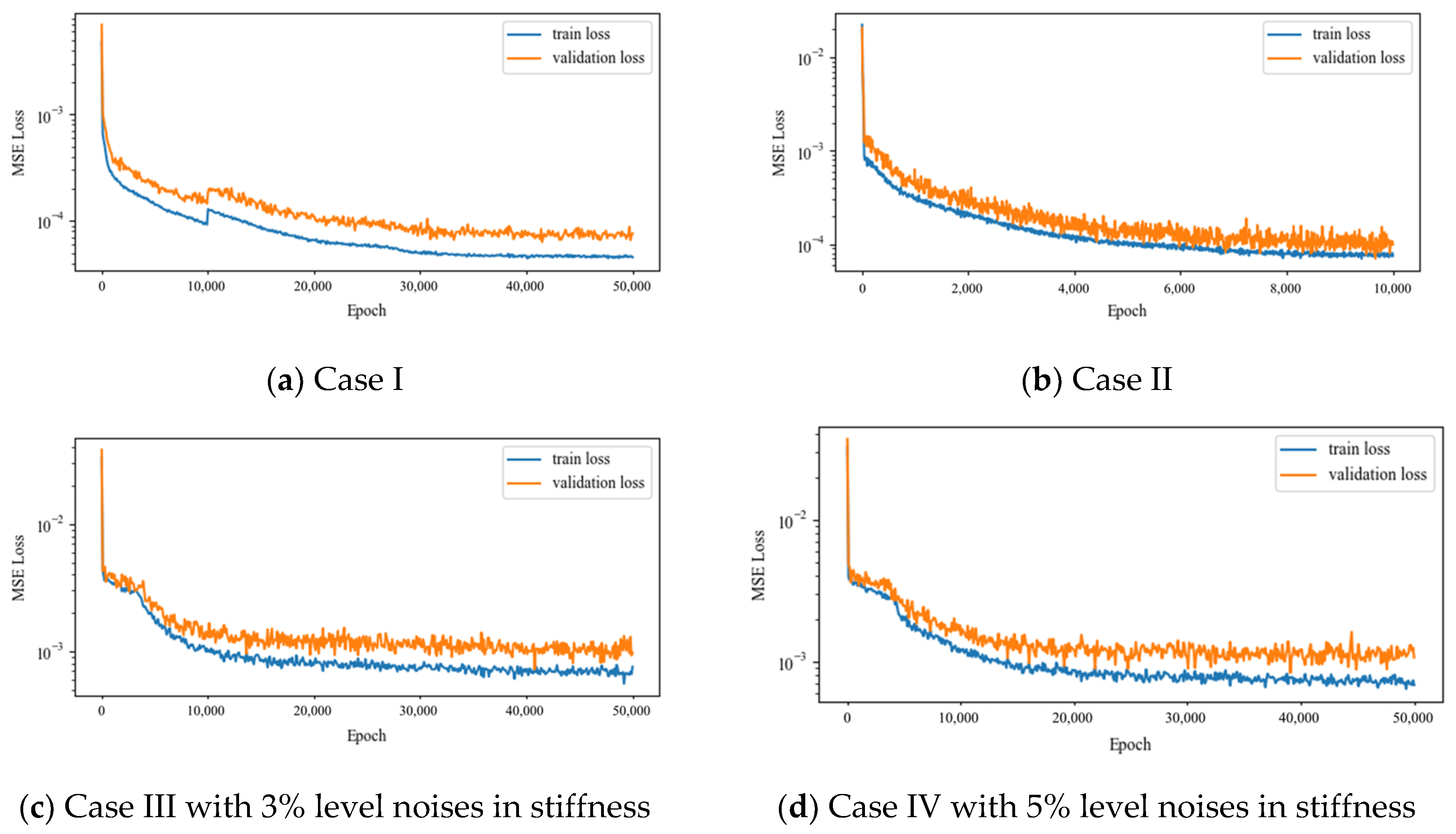
The training and validation loss during training for all cases are shown in Figure 10, all reach the acceptable level. As illustrated in the figure, Case II with the perfect symmetry and data augmentations converges fast within 10K training steps, Case III with 3% and 5% noise level converges secondly, and Case I with no augmentations converges the last within 50K steps. This reveals that the convergence speed of the same DBN model is related to dataset quality, both the incompleteness and noises in the dataset could harm the convergence: compared with Case II with the perfect symmetry and data augmentations, the incompleteness dataset without augmentations in Case I may introduce imbalance in the dataset that harm the convergence speed, and the imperfect symmetry in Case III and IV may introduce noises and complexity in the dataset that harm the convergence speed.

Meanwhile, the minimum training and validation loss for all cases is 1.5 × 10⁻⁵ and 2.6 × 10⁻⁵, 2.4 × 10⁻⁵ and 3.9 × 10⁻⁵, 1.1 × 10⁻⁴ and 2.1 × 10⁻⁴, 1.3 × 10⁻⁴ and 2.2 × 10⁻⁴ respectively. The training and validation losses for Case I are the least in all cases, which is due to the reduced data complexity with no augmentations, and the DBN model with the same capacity is able to model the dataset with a higher accuracy. The training and validation losses for Case IV are the highest in all cases, which is due to the increased data complexity of the imperfect symmetry. The minimum training and validation losses for Case III are lower than Case IV, indicating that the noises level in the stiffness and the higher asymmetry could harm the model accuracy.

(2)

Results on validation set

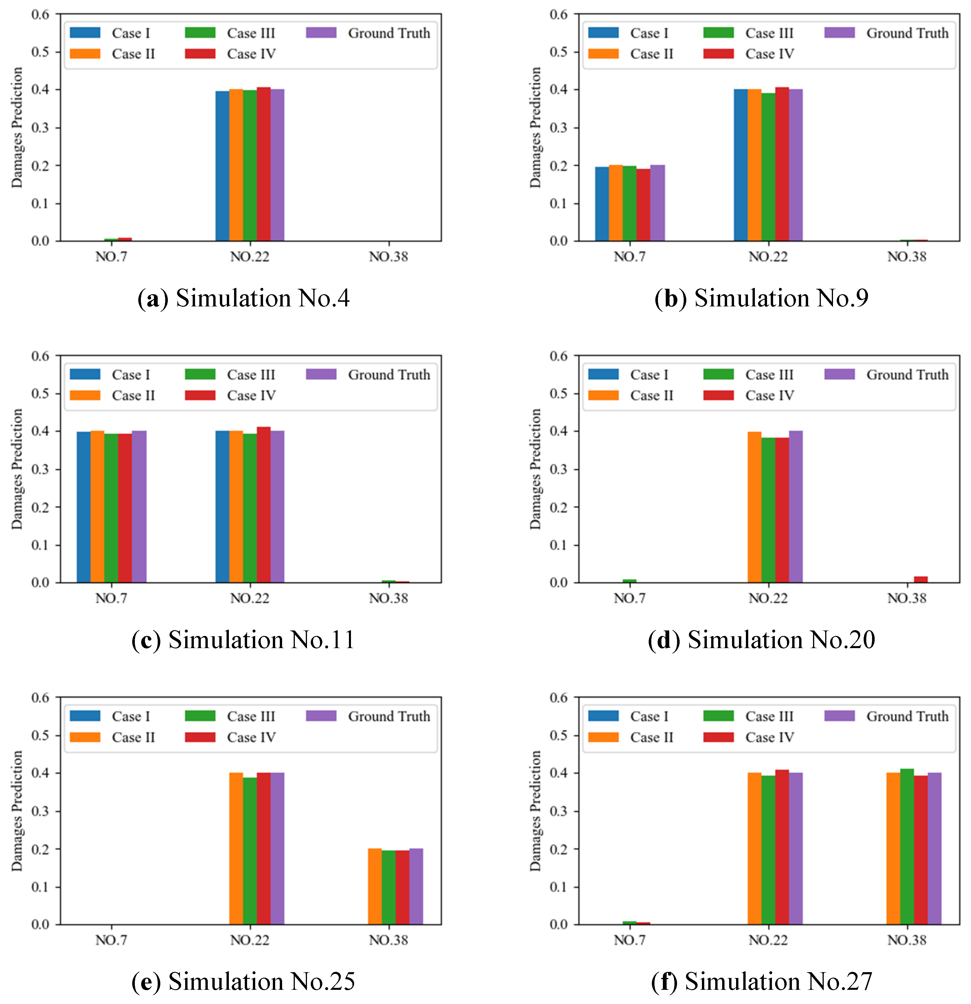
Results on the selected validation dataset (No. 4/9/11/20/25/27 in Table 2) for all four cases are shown in Figure 11 and

Table 3. Damage identification results for the validation set.

No.	Case I			Case II			Ground Truth
	7	22	38	7	22	38	7	22	38
12	0	0.396	0	0	0.399	0	0	0.4	0
13	0.195	0.400	0	0.201	0.400	0	0.2	0.4	0
14	0.397	0.399	0	0.400	0.401	0	0.4	0.4	0
15	-	-	-	0	0.399	0	0	0.4	0
16	-	-	-	0	0.401	0.199	0	0.4	0.2
17	-	-	-	0	0.399	0.399	0	0.4	0.4
No.	Case III			Case IV			Ground Truth
	7	22	38	7	22	38	7	22	38
12	0.004	0.398	0	0.008	0.406	0	0	0.4	0
13	0.198	0.390	0.003	0.190	0.406	0.004	0.2	0.4	0
14	0.392	0.393	0.004	0.394	0.410	0.004	0.4	0.4	0
15	0.009	0.381	0	0	0.381	0.017	0	0.4	0
16	0	0.387	0.194	0	0.400	0.194	0	0.4	0.2
17	0.007	0.392	0.401	0.005	0.408	0.393	0	0.4	0.4

. Note that damages on element No. 38 are not included in the original dataset, subfigures (e,f) validate the performance of the DBN model on the unseen data. And simulations no. 20, 25 and 27 are not included in the training set of Case I, thus subfigures (d–f) have no prediction results of Case I.

Results demonstrate that all models are well-trained on the given training dataset, and the prediction error is low on the randomly selected validation set. For Cases II, III, and IV with the data augmentation in the training set, the generalization to the unseen damage on element No. 38 is reliable. Meanwhile, results of Case III and Case IV have some false positive predictions in simulations 4, 9, 11, 20, and 27, where the target elements are not damaged but predicted to have minor damages. And the accuracy for the imperfect symmetric Cases III and IV also decrease compared to the perfect symmetric Cases I and II.

(3)

Results on test set

Results on the selected validation dataset and the test dataset for all four cases are shown in Figure 12 and

Table 4. Damage identification results on test set.

No.	Case I: Loss = 1.2 × 10−2			Case II: Loss = 1.5 × 10−4			Ground Truth
	7	22	38	7	22	38	7	22	38
12	0.006	0.102	0	0.006	0.102	0	0	0.1	0
13	0	0.501	0	0	0.501	0	0	0.5	0
14	0.216	0.003	0	0.216	0.003	0	0.2	0	0
15	0.416	0	0	0.417	0	0	0.4	0	0
16	0.169	0.136	0	0.189	0.212	0.205	0.2	0.2	0.2
17	0.362	0.271	0	0.401	0.399	0.410	0.4	0.4	0.4
No.	Case III: Loss = 2.6 × 10−4			Case IV: Loss = 3.4 × 10−4			Ground Truth
	7	22	38	7	22	38	7	22	38
12	0.002	0.103	0	0.002	0.108	0.010	0	0.1	0
13	0.001	0.494	0	0.005	0.480	0	0	0.5	0
14	0.196	0.032	0.011	0.195	0.017	0.015	0.2	0	0
15	0.387	0.010	0.001	0.401	0	0.030	0.4	0	0
16	0.186	0.184	0.217	0.173	0.187	0.211	0.2	0.2	0.2
17	0.362	0.382	0.373	0.38	0.364	0.363	0.4	0.4	0.4

. Note that the damaged level in simulation No.12 and 13 are 10% and 50% on element No. 22, forms the extrapolation tasks for the proposed DBN model. Results in Figure 12a,b show a good performance of the DBN model in all four cases, indicating that the proposed DBN model is capable of dealing with this kind of extrapolation tasks in damage amplitude. However, performance of Case III and IV slightly decreases compared to Case I and II, revealing the influence of the imperfect symmetry. False positive predictions are also found in simulation No. 14 and 15, as can be seen in Figure 12c,d.

It’s apparent that the well-trained DBN model in Case I failed to generalize to the unseen damages in Element No. 38 when the training dataset does not contain the augmented damage simulations. Meanwhile, other cases (Cases II, III and IV) generalize well to these unseen data, as shown in Figure 12e,f, indicating that the proposed DBN model is able to generalize the unseen damage cases when augmented properly.

Though in Case III and IV, the simulation dataset is based on the imperfect symmetric FE model with random noises on the stiffness of each element, the prediction results show robustness to this imperfect symmetry with data augmentation, the prediction MSE losses reach 2.6 × 10⁻⁴ and 2.6 × 10⁻⁴ respectively. In real-world applications, perfect symmetry is always not guaranteed, and imperfect symmetry is usually presented as the random noises in stiffness, mass and length of the ideal structure model. While it is still hard to theoretically prove the effectiveness of the symmetry-based data augmentation facing real-world imperfect symmetry, a possible explanation is that this type of imperfect symmetry is randomly distributed on the whole structure. These random noises in stiffness leads to an unbiased dataset with high variance, but the degraded stiffness in the damaged node is essentially an introductive bias to the structure. This alleviates the influence of the nonideal assumption and leads a plausible and practicable model for real-world applications.

4. Conclusions

This study discusses the generalization issue in data-driven methods for damage identification under limited data in the SHM field, we demonstrate and verify three possible approaches to alleviate this issue, corresponding to three key steps in the data-driven SHM methods. Following conclusions are obtained.

(1)

Physics-based data augmentation: Employing physics-based data augmentation in the data collection step proves beneficial in enhancing the diversity of the training dataset. This augmentation, utilizing the symmetry property of the structure, is verified as effective in expanding the dataset and diversifying the dataset distribution. The result shows the generalization ability of the proposed model to previously unseen data.

(2)

Preference for Physics-Based Features: Physics-based features with physical explainability are preferred rather than the end-to-end learned features in the feature selection step for generalization for the data-driven DL method. In this study, damage indicator derived from mode parameters is illustrated to be effective to reflect the damage location and the damage level explicitly, thus enhancing the accuracy and generalization ability of damage identification on incomplete datasets.

(3)

Efficient Generative Model Selection: The damage identification can be naturally modeled as a probabilistic inference process, and the DBN-based method can robustly learn the underlying distribution of input data in an efficient way. The overfitting issue is not present in the conductions, and results show good performance and generalization ability to the unseen new damage.