
Soil Condition Classification Based on Natural Water Content Using Computer Vision Technique


Abstract
1. Introduction
2. Experiment for Obtaining the Dataset
2.1. Problem Statement
2.2. Construction Site Information
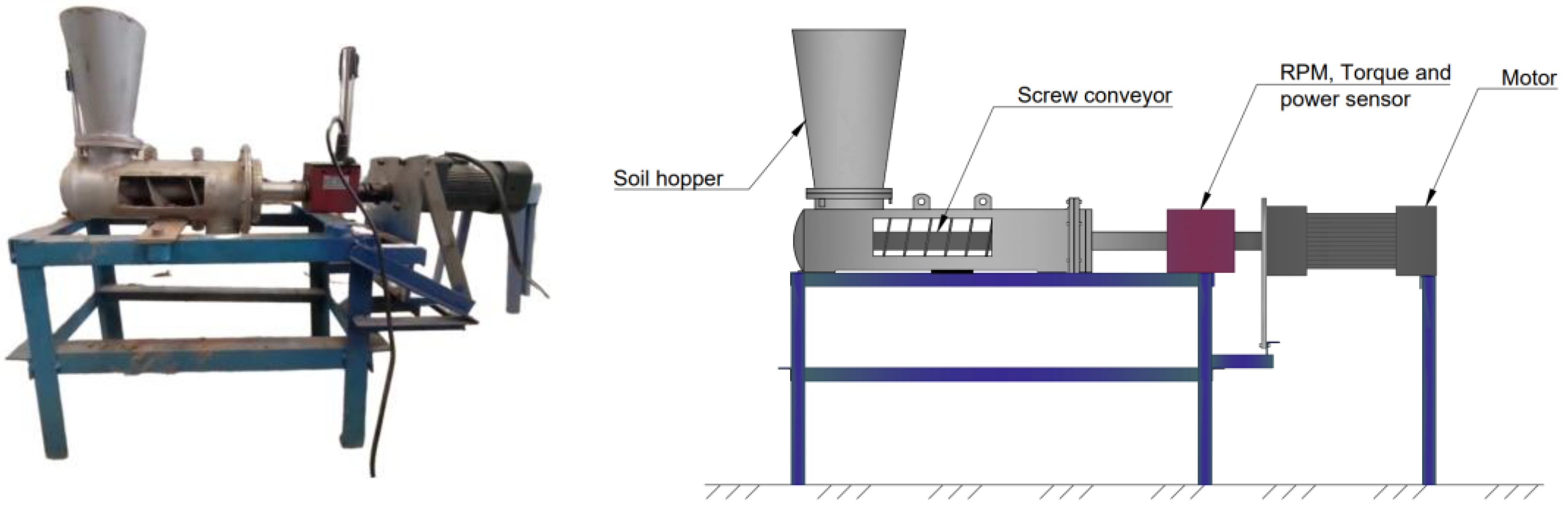
2.3. Experiment
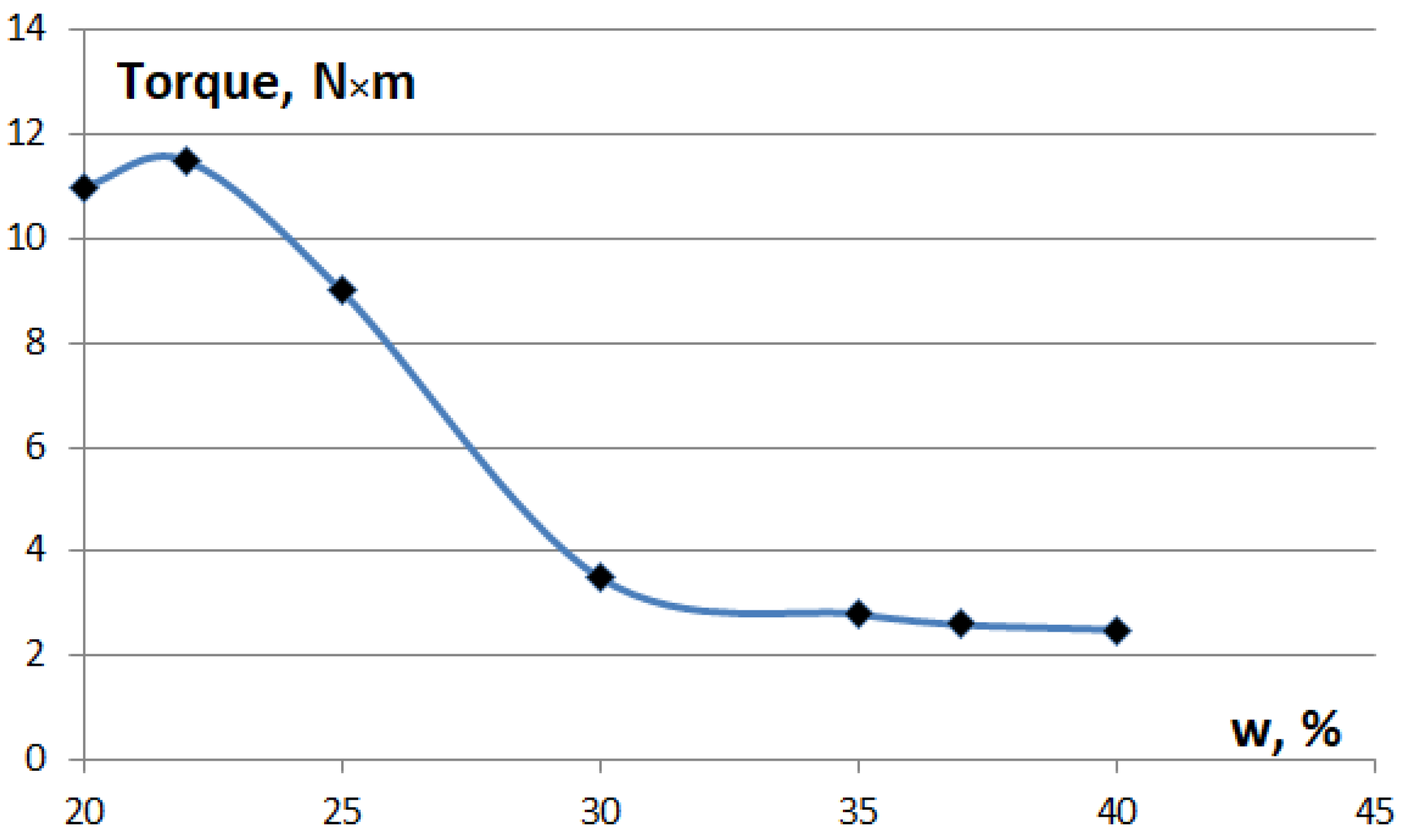
2.4. Interpretation of Intermediate Results
3. Deep Learning with CNN for Solving Computer Vision Problem of Classification
3.1. Main Concepts
3.2. Transfer Learning
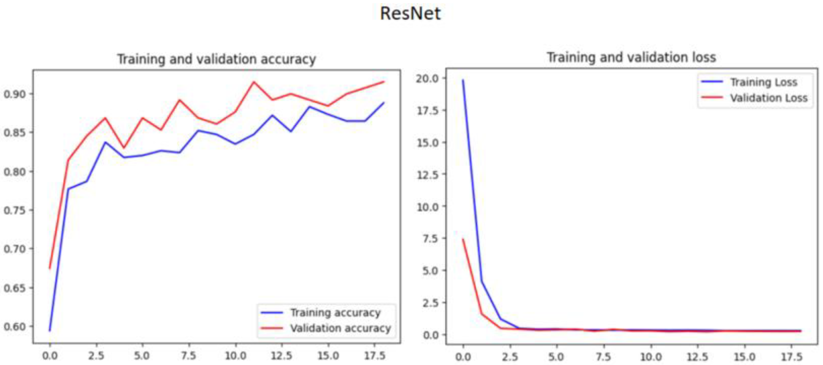
3.2.1. ResNet
3.2.2. MobileNet
3.2.3. Xception
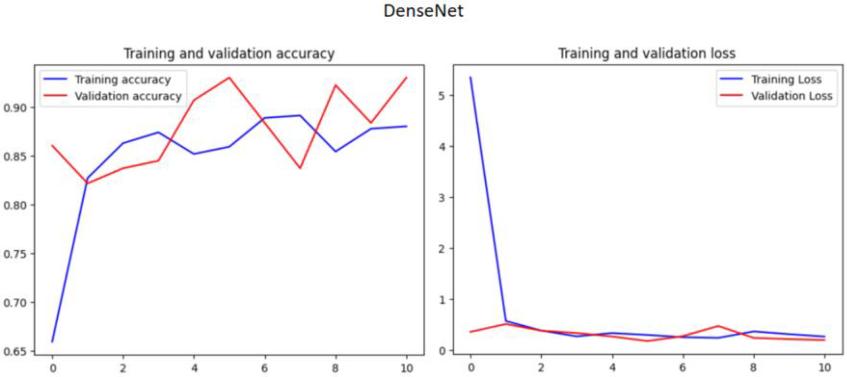
3.2.4. DenseNet
3.2.5. NasNet
3.2.6. EfficientNet
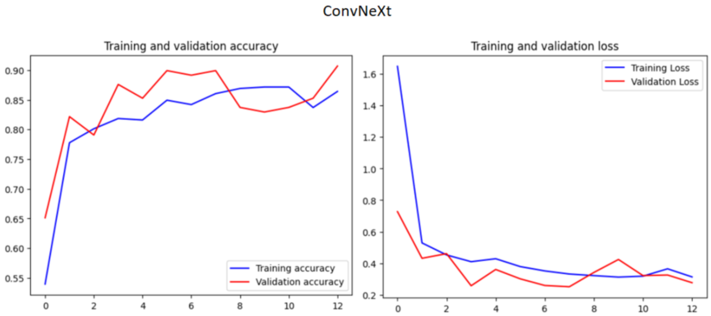
3.2.7. ConvNeXt [55]
3.3. Estimation and Optimization of the Models
3.4. Dataset
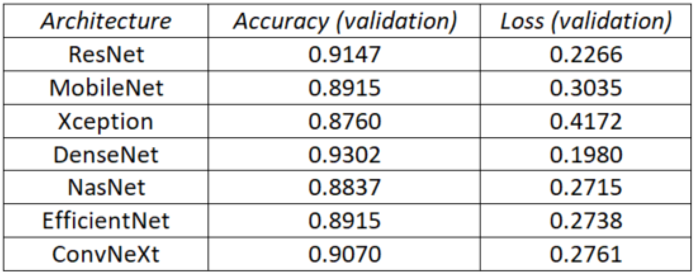
3.5. Results and Discussion
4. Conclusions
Author Contributions
Funding
Data Availability Statement
Conflicts of Interest
Appendix A


References
- Yagiz, S.; Gokceoglu, C.; Sezer, E.; Iplikci, S. Application of two non-linear prediction tools to the estimation of tunnel boring machine performance. Eng. Appl. Artif. Intell. 2009, 22, 808–814. [Google Scholar] [CrossRef]
- Yagiz, S.; Karahan, H. Prediction of hard rock TBM penetration rate using particle swarm optimization. Int. J. Rock Mech. Min. Sci. Géoméch. Abstr. 2011, 48, 427–433. [Google Scholar] [CrossRef]
- Armaghani, D.J.; Faradonbeh, R.S.; Momeni, E.; Fahimifar, A.; Tahir, M.M. Performance prediction of tunnel boring machine through developing a gene expression programming equation. Eng. Comput. 2017, 34, 129–141. [Google Scholar] [CrossRef]
- Kilic, K.; Narihiro, O.; Ikeda, H.; Adachi, T.; Kawamura, Y. Soft Ground Micro TBM Jack Speed and Torque Prediction Using Machine Learning Models Through Operator Data and Micro TBM-log Data Synchronization. Sci. Rep. 2024, 14, 9728. [Google Scholar] [CrossRef]
- Fu, X.; Gong, Q.; Wu, Y.; Zhao, Y.; Li, H. Prediction of EPB Shield Tunneling Advance Rate in Mixed Ground Condition Using Optimized BPNN Model. Appl. Sci. 2022, 12, 5485. [Google Scholar] [CrossRef]
- Shan, F.; He, X.; Armaghani, D.J.; Zhang, P.; Sheng, D. Success and challenges in predicting TBM penetration rate using recurrent neural networks. Tunn. Undergr. Space Technol. 2022, 130, 104728. [Google Scholar] [CrossRef]
- Shang, W.; Li, Y.; Wei, H.; Qiu, Y.; Chen, C.; Gao, X. Prediction method of longitudinal surface settlement caused by double shield tunnelling based on deep learning. Sci. Rep. 2024, 14, 908. [Google Scholar] [CrossRef]
- Alzubaidi, F.; Mostaghimi, P.; Si, G.; Swietojanski, P.; Armstrong, R.T. Automated Rock Quality Designation Using Convolutional Neural Networks. Rock Mech. Rock Eng. 2022, 55, 3719–3734. [Google Scholar] [CrossRef]
- Cui, R.; Cao, D.; Liu, Q.; Zhu, Z.; Jia, Y. VP and VS prediction from digital rock images using a combination of U-Net and convolutional neural networks. Geophysics 2021, 86, MR27–MR37. [Google Scholar] [CrossRef]
- Chen, L.; Liu, Z.; Su, H.; Lin, F.; Mao, W. Automated rock mass condition assessment during TBM tunnel excavation using deep learning. Sci. Rep. 2022, 12, 1722. [Google Scholar] [CrossRef]
- Liu, Y.; Wang, D.; Hu, J.; Zhu, G. Classifying Rock Fragments Produced by Tunnel Boring Machine Using Optimized Convolutional Neural Network. Rock Mech. Rock Eng. 2023, 57, 1765–1780. [Google Scholar] [CrossRef]
- Xue, Z.; Chen, L.; Liu, Z.; Lin, F.; Mao, W. Rock segmentation visual system for assisting driving in TBM construction. Mach. Vis. Appl. 2021, 32, 77. [Google Scholar] [CrossRef]
- Chen, J.; Yang, T.; Zhang, D.; Huang, H.; Tian, Y. Deep learning based classification of rock structure of tunnel face. Geosci. Front. 2021, 12, 395–404. [Google Scholar] [CrossRef]
- Bao, H.; Liu, C.; Liang, N.; Lan, H.; Yan, C.; Xu, X. Analysis of large deformation of deep-buried brittle rock tunnel in strong tectonic active area based on macro and microcrack evolution. Eng. Fail. Anal. 2022, 138, 106351. [Google Scholar] [CrossRef]
- Fang, Y.; Yao, Y.; Song, T.; Wei, L.; Liu, P.; Zhuo, B. Study on disintegrating characteristics and mechanism of cutterhead mud-caking in cohesive strata. Bull. Eng. Geol. Environ. 2022, 81, 510. [Google Scholar] [CrossRef]
- Teixeira, J.; Correia dos Santos, R. Exploring the Applicability of Low-Cost Capacitive and Resistive Water Content Sensors onCompacted Soils. Geotech. Geol. Eng. 2021, 39, 2969–2983. [Google Scholar] [CrossRef]
- Nikolov, G.T.; Ganev, B.T.; Marinov, M.B.; Galabov, V.T. Comparative Analysis of Sensors for Soil Moisture Measurement. In Proceedings of the 2021 XXX International Scientific Conference Electronics (ET), Sozopol, Bulgaria, 15–17 September 2021; IEEE: New York, NY, USA, 2021; pp. 1–5. [Google Scholar]
- Gao, Z.; Zhu, Y.; Liu, C.; Qian, H.; Cao, W.; Ni, J. Design and Test of a Soil Profile Moisture Sensor Based on Sensitive Soil Layers. Sensors 2018, 18, 1648. [Google Scholar] [CrossRef]
- Robinson, D.A.; Campbell, C.S.; Hopmans, J.W.; Hornbuckle, B.K.; Jones, S.B.; Knight, R.; Ogden, F.; Selker, J.; Wendroth, O. Soil Moisture Measurement for Ecological and Hydrological Watershed-Scale Observatories: A Review. Vadose Zone J. 2008, 7, 358–389. [Google Scholar] [CrossRef]
- Russell, M.B.; Davis, F.E.; Bair, R.A. The Use of Tensio-Meters for Following Soil Moisture Conditions under Corn. J. Am. Soc. Agron. 1940, 32, 922–930. [Google Scholar] [CrossRef]
- Fleischhauer-Binz, E. Die Messung von Bodensaugkräften mit Tensiometern. Planta 1949, 37, 565–594. [Google Scholar] [CrossRef]
- Jayawardane, N.; Meyer, W.; Barrs, H. Moisture Measurement in a Swelling Clay Soil Using Neutron Moisture Meters. Soil Res. 1984, 22, 109–117. [Google Scholar] [CrossRef]
- Knadel, M.; Masís-Meléndez, F.; de Jonge, L.W.; Moldrup, P.; Arthur, E.; Greve, M.H. Assessing Soil Water Repellency of a Sandy Field with Visible near Infrared Spectroscopy. J. Near Infrared Spectrosc. 2016, 24, 215–224. [Google Scholar] [CrossRef]
- Katuwal, S.; Knadel, M.; Moldrup, P.; Norgaard, T.; Greve, M.H.; de Jonge, L.W. Visible–Near-Infrared Spectroscopy Can PredictMass Transport of Dissolved Chemicals through Intact Soil. Sci. Rep. 2018, 8, 11188. [Google Scholar] [CrossRef]
- Qin, A.; Ning, D.; Liu, Z.; Duan, A. Analysis of the Accuracy of an FDR Sensor in Soil Moisture Measurement under Laboratory and Field Conditions. J. Sensors 2021, 2021, 6665829. [Google Scholar] [CrossRef]
- Yiming, W.; Yandong, Z. Study on the Measurement of Soil Water Content Based on the Principle of Standing Wave Ratio. In Proceedings of the Beijing International Conference on Agriculture Engineering, Beijing, China, 14–17 December 1999. [Google Scholar]
- Xu, Y.; Yang, W.; Li, Z. Soil Water Sensor Based on Standing Wave Ratio Method of Design and Development. In Proceedings of the International Conference on Computer and Computing Technologies in Agriculture, Beijing, China, 16–19 September 2014; Springer: Berlin/Heidelberg, Germany, 2014; pp. 720–730. [Google Scholar]
- Tian, H.; Gao, C.; Zhang, X.; Yu, C.; Xie, T. Smart Soil Water Sensor with Soil Impedance Detected via Edge Electromagnetic Field Induction. Micromachines 2022, 13, 1427. [Google Scholar] [CrossRef]
- Tsai, P.-H.; Huang, Y.; Tai, J.-H. Estimating soil water content from thermal images with an artificial neural network. CATENA 2024, 241, 108029. [Google Scholar] [CrossRef]
- Usta, A. Prediction of soil water contents and erodibility indices based on artificial neural networks: Using topography and remote sensing. Environ. Monit. Assess. 2022, 194, 794. [Google Scholar] [CrossRef]
- Kim, D.; Kim, T.; Jeon, J.; Son, Y. Soil-Surface-Image-Feature-Based Rapid Prediction of Soil Water Content and Bulk Density Using a Deep Neural Network. Appl. Sci. 2023, 13, 4430. [Google Scholar] [CrossRef]
- Armetti, G.; Migliazza, M.R.; Ferrari, F.; Berti, A.; Padovese, P. Geological and mechanical rock mass conditions for TBM performance prediction. The case of “La Maddalena” exploratory tunnel, Chiomonte (Italy). Tunn. Undergr. Space Technol. 2018, 77, 115–126. [Google Scholar] [CrossRef]
- Fatemi, S.A.; Ahmadi, M.; Rostami, J. Evaluation of TBM performance prediction models and sensitivity analysis of input parameters. Bull. Eng. Geol. Environ. 2016, 77, 501–513. [Google Scholar] [CrossRef]
- Yagiz, S.; Karahan, H. Application of various optimization techniques and comparison of their performances for predicting TBM penetration rate in rock mass. Int. J. Rock Mech. Min. Sci. Géoméch. Abstr. 2015, 80, 308–315. [Google Scholar] [CrossRef]
- Xia, Y.; Yang, M.; Mei, Y.; Ji, Z. Influence of Geological Properties and Operational Parameters on TBM Muck Removal Performance for Yinsong Tunnel. Geotech. Geol. Eng. 2021, 40, 2291–2306. [Google Scholar] [CrossRef]
- Barla, G.; Pelizza, S. TBM tunnelling in difficult ground conditions. In Proceedings of the ISRM International Symposium, Melbourne, Australia, 19–24 November 2000. [Google Scholar]
- Broere, W. Tunnel Face Stability & New CPT Applications. Ph.D. Thesis, Technische Universiteit Delft, Delft, The Netherlands, 2001. [Google Scholar]
- Shirlaw, N. Setting operating pressures for TBM tunnelling. In Proceedings of the 32nd geotechnical division’s annual seminar, Hong Kong Institution of Engineers (HKIE), Hong Kong, 25 May 2012. [Google Scholar]
- Sitarenios, P.; Litsas, D.; Papadakos, A.; Kavvadas, M. Effect of Hydraulic Conditions in controlling the Face in EPB Excavated Tunnels. In Proceedings of the 2015 World Tunnel Congress, Dubrovnik, Croatia, 22–28 May 2015. [Google Scholar]
- Bouri, D.; Krim, A.; Brahim, A.; Arab, A. Shear strength of compacted Chlef sand: Effect of water content, fines content and others parameters. Stud. Geotech. Mech. 2020, 42, 18–35. [Google Scholar] [CrossRef]
- Dafalla, M.A. Effects of Clay and Moisture Content on Direct Shear Tests for Clay-Sand Mixtures. Adv. Mater. Sci. Eng. 2013, 2013, 562726. [Google Scholar] [CrossRef]
- Gusman, M.; Nazki, A.; Putra, R.R. The modelling influence of water content to mechanical parameter of soil in analysis of slope stability. J. Phys. 2018, 1008, 012022. [Google Scholar] [CrossRef]
- Stracke, F.; Jung, J.G.; Korf, E.P.; Consoli, N.C. The Influence of Moisture Content on Tensile and Compressive Strength of Artificially Cemented Sand. Soils Rocks 2012, 35, 303–308. [Google Scholar] [CrossRef]
- Bao, H.; Song, Z.; Lan, H.; Ma, Y.; Yan, C.; Liu, S. Analysis of the mechanical effects and influencing factors of cut-fill interface within loess subgrade. Eng. Fail. Anal. 2024, 163, 108488. [Google Scholar] [CrossRef]
- Ye, C.; Guo, Z.; Cai, C.; Wang, J.; Deng, J. Effect of water content, bulk density, and aggregate size on mechanical characteristics of Aquults soil blocks and aggregates from subtropical China. J. Soils Sediments 2016, 17, 210–219. [Google Scholar] [CrossRef]
- Liu, S.; Wen, C.; Cheng, P.; Zhang, Z.; Wu, Z. Experimental Study on Strength Characteristics of Soil-Rock Mixture Under Different Water Contents; IOS Press: Amsterdam, The Netherlands, 2023. [Google Scholar] [CrossRef]
- Mohamad, E.; Alshameri, B.; Kassim, K.; Saad, R. Shear Strength Behaviour for Older Alluvium Under Different Moisture Content. Electron. J. Geotech. Eng. 2011, 16, 605–617. [Google Scholar]
- Zhou, F.-Y.; Jin, L.; Dong, J. Review of Convolutional Neural Network. Jisuanji Xuebao/Chin. J. Comput. 2017, 40, 1229–1251. [Google Scholar]
- He, K.; Zhang, X.; Ren, S.; Sun, J. Deep Residual Learning for Image Recognition. In Proceedings of the 2016 IEEE Conference on Computer Vision and Pattern Recognition (CVPR), Las Vegas, NV, USA, 26 June–1 July 2016; pp. 770–778. [Google Scholar] [CrossRef]
- Andrew, H.; Menglong, Z.; Bo, C.; Dmitry, K.; Weijun, W.; Tobias, W.; Marco, A.; Hartwig, A. MobileNets: Efficient Convolutional Neural Networks for Mobile Vision Applications. arXiv 2017, arXiv:1704.04861. [Google Scholar]
- Chollet, F. Xception: Deep Learning with Depthwise Separable Convolutions. In Proceedings of the 30th IEEE Conference on Computer Vision and Pattern Recognition (CVPR), Honolulu, HI, USA, 21–26 July 2017; pp. 1800–1807. [Google Scholar]
- Huang, G.; Liu, Z.; Van Der Maaten, L.; Weinberger, K.Q. Densely Connected Convolutional Networks. In Proceedings of the 2017 IEEE Conference on Computer Vision and Pattern Recognition, Honolulu, HI, USA, 21–26 July 2017; pp. 2261–2269. [Google Scholar] [CrossRef]
- Zoph, B.; Vasudevan, V.; Shlens, J.; Le, Q.V. Learning Transferable Architectures for Scalable Image Recognition. In Proceedings of the 2018 IEEE/CVF Conference on Computer Vision and Pattern Recognition, Salt Lake City, UT, USA, 18–23 June 2018; pp. 8697–8710. [Google Scholar] [CrossRef]
- Tan, M.; Le, Q. EfficientNet: Rethinking Model Scaling for Convolutional Neural Networks. arXiv 2019, arXiv:1905.11946. [Google Scholar] [CrossRef]
- Liu, Z.; Mao, H.; Wu, C.-Y.; Feichtenhofer, C.; Darrell, T.; Xie, S. A ConvNet for the 2020s. arXiv 2022, arXiv:2201.03545. [Google Scholar] [CrossRef]
- Russakovsky, O.; Deng, J.; Su, H.; Krause, J.; Satheesh, S.; Ma, S.; Huang, Z.; Karpathy, A.; Khosla, A.; Bernstein, M.; et al. ImageNet Large Scale Visual Recognition Challenge. Int. J. Comput. Vis. 2015, 115, 211–252. [Google Scholar] [CrossRef]


| Confusion Matrix | |||
|---|---|---|---|
| Class I | 22 | 1 | 1 |
| Class II | 3 | 22 | 1 |
| Class II | 3 | 3 | 75 |
| Class I | Class II | Class III | |
Disclaimer/Publisher’s Note: The statements, opinions and data contained in all publications are solely those of the individual author(s) and contributor(s) and not of MDPI and/or the editor(s). MDPI and/or the editor(s) disclaim responsibility for any injury to people or property resulting from any ideas, methods, instructions or products referred to in the content. |
© 2025 by the authors. Licensee MDPI, Basel, Switzerland. This article is an open access article distributed under the terms and conditions of the Creative Commons Attribution (CC BY) license (https://creativecommons.org/licenses/by/4.0/).
Share and Cite
Miller, M.; Fang, Y.; Wang, Y.; Kharitonov, S.; Akulich, V. Soil Condition Classification Based on Natural Water Content Using Computer Vision Technique. Infrastructures 2025, 10, 138. https://doi.org/10.3390/infrastructures10060138
Miller M, Fang Y, Wang Y, Kharitonov S, Akulich V. Soil Condition Classification Based on Natural Water Content Using Computer Vision Technique. Infrastructures. 2025; 10(6):138. https://doi.org/10.3390/infrastructures10060138
Chicago/Turabian StyleMiller, Mark, Yong Fang, Yubo Wang, Sergey Kharitonov, and Vladimir Akulich. 2025. "Soil Condition Classification Based on Natural Water Content Using Computer Vision Technique" Infrastructures 10, no. 6: 138. https://doi.org/10.3390/infrastructures10060138
APA StyleMiller, M., Fang, Y., Wang, Y., Kharitonov, S., & Akulich, V. (2025). Soil Condition Classification Based on Natural Water Content Using Computer Vision Technique. Infrastructures, 10(6), 138. https://doi.org/10.3390/infrastructures10060138