Seismic Reliability Analysis of Highway Pile–Plate Structures Considering Dual Stochasticity of Parameters and Excitation via Probability Density Evolution

Abstract

The paper innovatively studies the impact of dual randomness of structural parameters and seismic excitation on the seismic reliability of highway pile–slab structures using the probability density evolution method. A nonlinear stochastic dynamic model was established through the platform, integrating, for the first time, the randomness of concrete material properties and seismic motion variability. The main findings include the following: Under deterministic seismic input, the displacement angle fluctuation range caused by structural parameter randomness is ±3%, and reliability decreases from 100% to 65.26%. For seismic excitation randomness, compared to structural parameter randomness, reliability at the 3.3% threshold decreases by 7.99%, reaching 92.01%. Dual randomness amplifies the variability of structural response, reducing reliability to 86.38% and 62%, with a maximum difference of 20.5% compared to single-factor scenarios. Compared to the Monte Carlo method, probability density evolution shows significant advantages in computational accuracy and efficiency for large-scale systems, revealing enhanced discreteness and irregularity under combined randomness. This study emphasizes the necessity of addressing dual randomness in seismic design, advancing probabilistic seismic assessment methods for complex engineering systems, thereby aiding the design phase in enhancing facility safety and providing scientific basis for improved design specifications.

1. Introduction

At present, the supply of land resources in highway construction is becoming increasingly tight, and the prominent contradiction of having no land to occupy and no soil to rely on has been observed. A pile–plate structure, which is a frame structure system composed of a factory prefabricated plate girder and pipe pile, exhibits several advantages such as resource saving, cost reduction, and high industrialization. As opposed to the traditional fill roadbed, it features large stiffness and small settlement after construction, effectively addressing issues related to difficult land acquisition and large quantities of fill. Nevertheless, many pile–plate structures pass through regions with high seismic intensity, thereby exposing them to the risk of major engineering safety problems resulting from seismic hazards. In seismic disasters, the severe damage to bridge engineering not only causes enormous economic losses and social impacts but also severs the transportation lifelines in the affected areas. For instance, the 1989 Loma Prieta earthquake resulted in hundreds of casualties, economic losses of USD 7 billion, and the collapse of the Cypress Freeway overpass. The 1995 Great Hanshin (Kobe) earthquake in Japan caused nearly 6300 fatalities, economic losses of a record USD 100 billion, severed transportation networks, and required nearly USD 100 billion and 2 years for post-disaster recovery and reconstruction [1]. Thus, there is an urgent practical need for carrying out in-depth seismic analysis and reliability research of pile–plate structures.

Currently, the seismic analysis of pile–slab structures has not adequately considered the influence of randomness on their structural behavior. In fact, both the physical parameters of such structures and seismic excitations possess stochastic characteristics. Concrete, as a multiphase composite material, exhibits stochastic mechanical properties primarily due to the coupling effects of construction environments, construction sequences, and the random spatial distribution of aggregates. The random distribution of aggregates is a key factor causing stochastic variations in concrete materials, affecting the formation of initial microcracks, the propagation of damage, and subsequent changes in mechanical properties [2,3,4,5]. According to research studies by Feng et al., the randomness of concrete results in significant fluctuations in the nonlinear response of reinforced concrete frames [6]. During strong earthquakes, this unpredictability of concrete materials leads to various collapse modes, significantly influencing seismic design [7,8]. To address this issue, Zeng et al. [9] proposed a stochastic prediction model for the crack extension process of concrete that investigates the effect of concrete inhomogeneity on crack opening displacement, fracture process, and crack extension trajectory. Additionally, Feng et al. [10] developed a multi-scale stochastic damage model for concrete and applied it to the stochastic response analysis of reinforced concrete shear wall structures, reflecting the effect of stochasticity from the material level to the structural level. On the other hand, seismic excitation is inherently stochastic due to variations in its source, propagation path, and site environment [11,12,13]. An earthquake can be considered a highly intricate stochastic process with non-stationary time and frequency features. The limited artificially selected ground-shaking simulations fail to cover the stochastic behavior of naturally occurring earthquakes. Currently, most of the analyses on seismic performance of structures rely on a particular natural seismic wave and use the finite element method to solve the problem [14,15,16], which poses challenges in objectively and comprehensively characterizing such performance as well as the dynamic damage mechanisms of presiding structures [17,18,19]. In a previous study conducted by Li J et al. [20], a method was proposed to generate ground-shaking samples based on a random function model with probabilistic description of the generated ground-shaking samples using “source–propagation path–local site” mechanism that considers the variability of the used source parameters. Based on this, the stochastic seismic response and reliability of structures were evaluated using a non-stationary ground-shaking stochastic process orthogonal expansion model and probability density evolution theory [21,22].

To ensure the disaster-resistance safety of engineering structures, it is necessary to conduct nonlinear response and reliability analyses of engineering structures with stochastic parameters under stochastic dynamic excitations. Specifically, classical stochastic simulation methods and their improvement techniques have gained attention from scholars both at home and abroad [23,24]. Progress has been made in the examination of stochastic reactions of linear and nonlinear multi-degree-of-freedom structural systems, computing dynamic and system dependability and reliability-based regulation [25,26,27]. Although these studies have indeed improved the computational efficiency of the Monte Carlo method, there are still unresolved difficulties in the analysis of non-stationary responses of general nonlinear dynamic systems. The theory of stochastic structural analysis has generally formed three types of stochastic structural analysis methods: stochastic perturbation theory, stochastic simulation methods, and orthogonal expansion theory [28]. All these methods reflect the probabilistic characteristics of structural responses by grasping the numerical features of structural response quantities, but they fail to comprehensively reflect the probabilistic information of structural response quantities and encounter difficulties in dealing with the coupling of nonlinearity and stochasticity, thus being unable to effectively solve the problem of nonlinear stochastic dynamic response analysis of structures. Based on the fundamental concept of physical stochastic systems, the probability density evolution theory holds promise for solving a series of problems in the analysis and control of nonlinear stochastic dynamic systems. Li and Chen [29,30,31,32,33] have made noteworthy contributions to probability density development of stochastic systems by deriving a generalized probability density evolution equation based on the principle of probability conservation. Furthermore, they proposed a numerical solution method to calculate structural dynamic reliability through the imposition of boundary conditions. This method presents a brand-new avenue for the resolution of the stochastic vibration problem, boasting high accuracy and efficiency. Consequently, it can significantly improve the computational efficiency of structural dynamic reliability analysis of large complex projects while efficiently resolving many problems in the analysis and control of current nonlinear stochastic dynamic systems [34,35,36,37].

In the design of pile–slab structures, the existing literature is mostly limited to single-factor analysis and lacks quantitative assessments of the coupling effects of composite stochasticity. Research on the dual stochasticity of highway pile–slab structures remains a void, yet fully considering the stochasticity of concrete materials and seismic excitations is significant for the seismic analysis of pile–slab structures. To address this, this paper, for the first time, implements the nonlinear dynamic response and reliability analysis of pile–slab structures under dual stochasticity using the probability density evolution method and elucidates the mechanism by which the superposition of stochasticity leads to a significant decrease in reliability, thereby aiding in enhancing facility safety at the design stage and providing a scientific basis for improving design specifications.

2. Methodology

Li J and Chen J B have proposed a probability density evolution theory based on the study of physical stochastic systems, employing the generalized probability density evolution equation as the core [38,39]. This approach unifies randomness arising from internal and external parameters in physical stochastic dynamical systems, yielding more accurate descriptions of the propagation law of randomness in engineering systems. Additionally, this theory provides a perspective for tackling reliability problems that arise due to stochastic factors in complex engineering structures. Compared with specific deterministic analysis, this method can accurately predict the response of pile–plate structures to seismic forces, reduce the possibility of structural failure during earthquakes, and prevent or minimize damage caused by earthquakes.

2.1. Probability Density Evolution Equation

Considering the influence of internal and external stochastic factors, the motion equation of a multi-degree-of-freedom nonlinear dynamic system can be expressed as shown in Equation (1):

$$M\left(\mathsf{\Phi }\right)\ddot{U}\left(t\right)+C\left(\mathsf{\Phi }\right)\dot{U}\left(t\right)+f\left(\mathsf{\Phi },U(t)\right)=F(\mathsf{\Phi },\mathrm{t})$$

(1)

In this formula, $M$ is the mass matrix, $C$ is the damping matrix, $f\left(\mathsf{\Phi },U\right)$ is the restoring force vector, and $F(\mathsf{\Phi },\mathrm{t})$ is the external load vector. $\ddot{U}\left(t\right),\dot{ U}\left(t\right)$ and $U\left(t\right)$ are the acceleration, velocity, and displacement vectors of the system reaction, respectively, $\mathsf{\Phi }=({\mathsf{\Phi }}_1,{\mathsf{\Phi }}_2,\cdots ,{\mathsf{\Phi }}_n)$ denotes the vector of random parameters in the system, $X={(X_1,X_2,\cdots ,X_m)}^{\mathrm{T}}$ denotes the physical response of the system to be found, $(X,\mathsf{\Phi })$ denotes the vector of incremental states in the system, and its joint probability density function satisfies the following equation [40,41]:

$${\displaystyle \frac{\partial p_{X\Phi }(x,\phi ,t)}{\partial t}}+\sum _{i=1}^m{\dot{X}}_i(\phi ,t){\displaystyle \frac{\partial p_{X\Phi }(x,\phi ,t)}{\partial x_i}}=0$$

(2)

The initial condition of Equation (2) is:

$${p_{X\Phi }(x,\phi ,t)|}_{t=0}=\delta (x-x_0)p_{\Phi }(\phi )$$

(3)

In this formula, $p_{X\Phi }$ is the transition probability density function, ${\displaystyle \frac{\partial }{\partial t}}$ is the derivative, and $x_0$ is a deterministic initial value.

This is solved to obtain Equation (4):

$$p_X(x,t)={\int }_{{\Omega }_0}{p}_{X\Phi }(x,\phi ,t)d\phi$$

(4)

where ${\Omega }_{\Phi }$ denotes the probability space of $\mathsf{\Phi }$.

Equation (1) can be simplified to a one-element partial differential equation when only a random physical quantity is considered:

$${\displaystyle \frac{\partial {\rho }_{X\Phi }\left(x,\phi ,t\right)}{\partial t}}+\dot{X}\left(\phi ,t\right){\displaystyle \frac{\partial {\rho }_{X\Phi }\left(x,\phi ,t\right)}{\partial x}}=0$$

(5)

By employing the probability density evolution equation, it is possible to relate the stochastic factors inside and outside the structure with deterministic parameters. On this basis, solving the probability density evolution equation for structural reliability analysis can be achieved.

2.2. Solution of the Evolution Equation of Probability Density

Generally, by combining the physical Equation (1) with the probability density evolution Equation (2) and solving them, the probability density function of the structural response during a certain period of time can be obtained. The specific solution process includes the following steps:

Firstly, the probability interval of the basic random variable $\mathsf{\Phi }$ is partitioned to obtain the subdomain ${\Omega }_{{\phi }_q}$ of the probability space. In the subdomain ${\Omega }_{{\phi }_q}$, discrete representative points ${\phi }_q=\left({\phi }_{1,q},{\phi }_{2,q},\cdots ,{\phi }_{s,q}\right),$ q = 1, 2, $\cdots$, $n_{sel}$, are selected. Here, $n_{sel}$ is the number of chosen discrete representative points, and this step can be used to ensure the uniformity of the selected representative point set. The assigned probability of each representative point can be determined by $P_q={\int }_{V_q}{p}_{\Phi }\left(\phi \right)d\phi$, where $V_q$ is the representative volume.

Then, the deterministic dynamical system is solved for the given $\Phi ={\phi }_q$ and the time inverse of the corresponding physical quantity ${\dot{X}}_i\left({\phi }_q,t\right)$, $i$ = 1, 2, $\cdots$, m, is obtained. After determining the selected discrete representative points and the corresponding assigned probabilities for each point, Equation (2) becomes:

$${\displaystyle \frac{\partial p_{X\Phi }\left(x,{\phi }_q,t\right)}{\partial t}}+\sum _{i=1}^m{\dot{X}}_i\left({\phi }_q,t\right){\displaystyle \frac{\partial p_{X\Phi }\left(x,{\phi }_q,t\right)}{\partial x_i}}=0$$

(6)

The corresponding initial condition (3) becomes:

$$p_{X\Phi }{\left.\left(x,{\phi }_q,t\right)\right|}_{t=t_0}=\delta \left(x-x_0\right)p_q$$

(7)

The joint probability density function $p_{X\Phi }\left(x,{\phi }_q,t\right)$ of $\left(X,\Phi \right)$ is obtained by substituting the time inverse of the relevant physical quantities ${\dot{X}}_i\left({\phi }_q,t\right)$ obtained previously into Equation (6) and solving it using the TVD finite difference method.

Finally, all $p_{X\Phi }\left(x,{\phi }_q,t\right),q=1, 2, \cdots , n_{sel}$ obtained in the previous step are summed cumulatively to obtain the numerical solution of the joint density function $p_X\left(x,t\right)$ of $X\left(t\right)$ as follows:

$$p_X\left(x,t\right)=\sum _{q=1}^{n_{sel}}{p}_{X\Phi }\left(x,{\phi }_q,t\right)$$

(8)

The process described above is the point evolution method for solving the generalized probability density evolution equation. This method reveals the mechanism by which the evolution of the probability density depends on the evolution of the physical state, i.e., the physical mechanism is the driving force of the stochastic propagation.

2.3. Structural Seismic Reliability Analysis Methods

Structural dynamic reliability refers to the probability that a structure can meet the expected response under specific time intervals, specific conditions, and the effects of random dynamic loads. The first-order reliability method is an important and effective criterion used to determine the structural dynamic reliability under different conditions. In the first-order reliability method, structural failure is defined as a random event, and the definition of structural dynamic reliability is the probability that the physical quantities (such as shear force, displacement, stress–strain, etc.) that cause structural failure within a specific time period do not exceed the safety threshold.

$$R(t)=\mathrm{P}\mathrm{r}\{X(\tau )\in {\Omega }_S,0\le \tau \le t\}$$

(9)

Here, $X(\tau )$ is the physical quantity causing the structural failure; ${\Omega }_S$ is the safety region, and it is assumed that the safety domain boundary $\partial {\Omega }_S$ does not change with time.

For the first time, the destructive criterion is exceeded: after crossing the failure boundary, the probability carried by the structural response irreversibly flows from the safe domain to the failure domain. At this point, the dynamic reliability of the structure is determined by the probability of random events staying within the safe domain. To assess this, the probability density evolution equation is solved using the absorption boundary conditions, resulting in the probability density function of the structure within the safe domain. Through integration, the dynamic reliability of the structure can be calculated.

According to the above definition, in a stochastic dynamic system $\left(X,\mathsf{\Phi }\right)$, when the structural dynamic response $X\left(t\right)$ exceeds its allowable value $\left[X\right]$ for the first time, the probability of the system undergoing dissipation will occur. In calculating the structural reliability using different failure criteria, the probability density evolution equation of the probabilistic dissipation system below can be used:

$${\displaystyle \frac{\partial p_{X\Phi }\left(x,\phi ,t\right)}{\partial t}}+\sum _{i=1}^m{\dot{X}}_i\left(\phi ,t\right){\displaystyle \frac{\partial p_{X\Phi }\left(x,\phi ,t\right)}{\partial X_i}}=-H\left[X\left(t\right)\right]\cdot p_{X\Phi }\left(x,\phi ,t\right)$$

(10)

where $H\left(·\right)$ is the sieve operator and represents the probability dissipation factor:

$$H\left[X\left(t\right)\right]=\left\{\begin{array}{c}0 X\left(t\right)\in {\Omega }_S\\ 1 X\left(t\right)\in {\Omega }_D\end{array}\right\}$$

(11)

where ${\Omega }_S$ is the structural safety domain, i.e., the region bounded by the allowed value $\left[X\right]$ of $X\left(t\right)$; and ${\Omega }_D$ is the structural failure domain, i.e., the probability dissipation domain; the probability density function of the system after probability dissipation occurs as:

$$p_X\left(x,t\right)={\int }_{{\Omega }_{\Phi }}{p}_{X\Phi }\left(X,\phi ,t\right)d\phi$$

(12)

Integrating the density function yields the probability that the system retains after dissipating energy at time t, which represents the dynamic reliability of the structure.

$$R\left(t\right)={\int }_{-\mathrm{\infty }}^{+\mathrm{\infty }}{p}_X\left(x,t\right)dx$$

(13)

The probabilistic structural reliability analysis based on the Probability Dissipation System is a universal method. As long as effective structure failure criteria are introduced as the physical mechanism driving the probability dissipation, the dynamic reliability of any structural system can be obtained. By combining the first exceedance failure criterion with the probability density evolution theory, the reliability of pile–plate structures can be calculated.

3. Seismic Reliability Analysis of Pile–Slab Structure Considering Randomness of Concrete

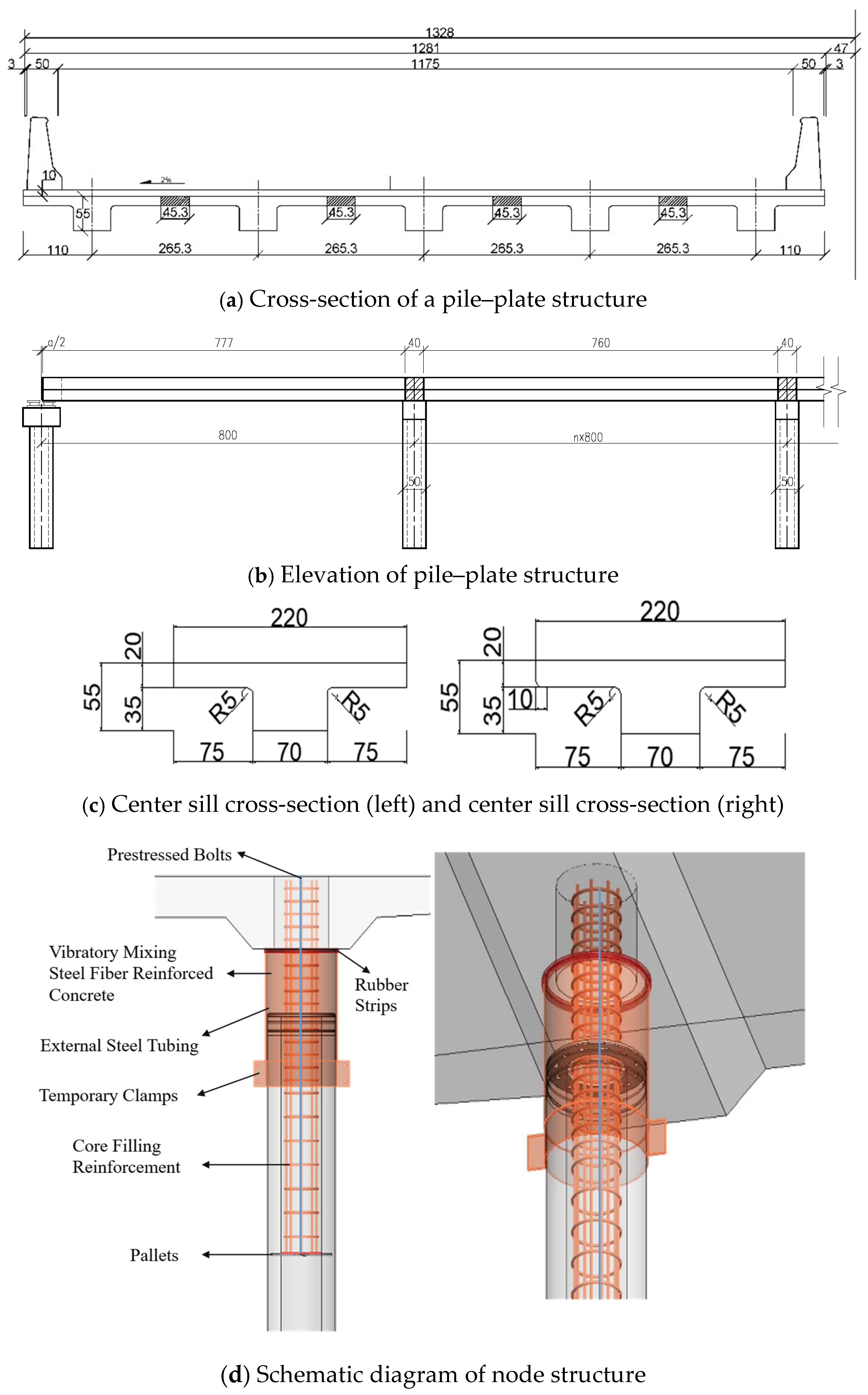
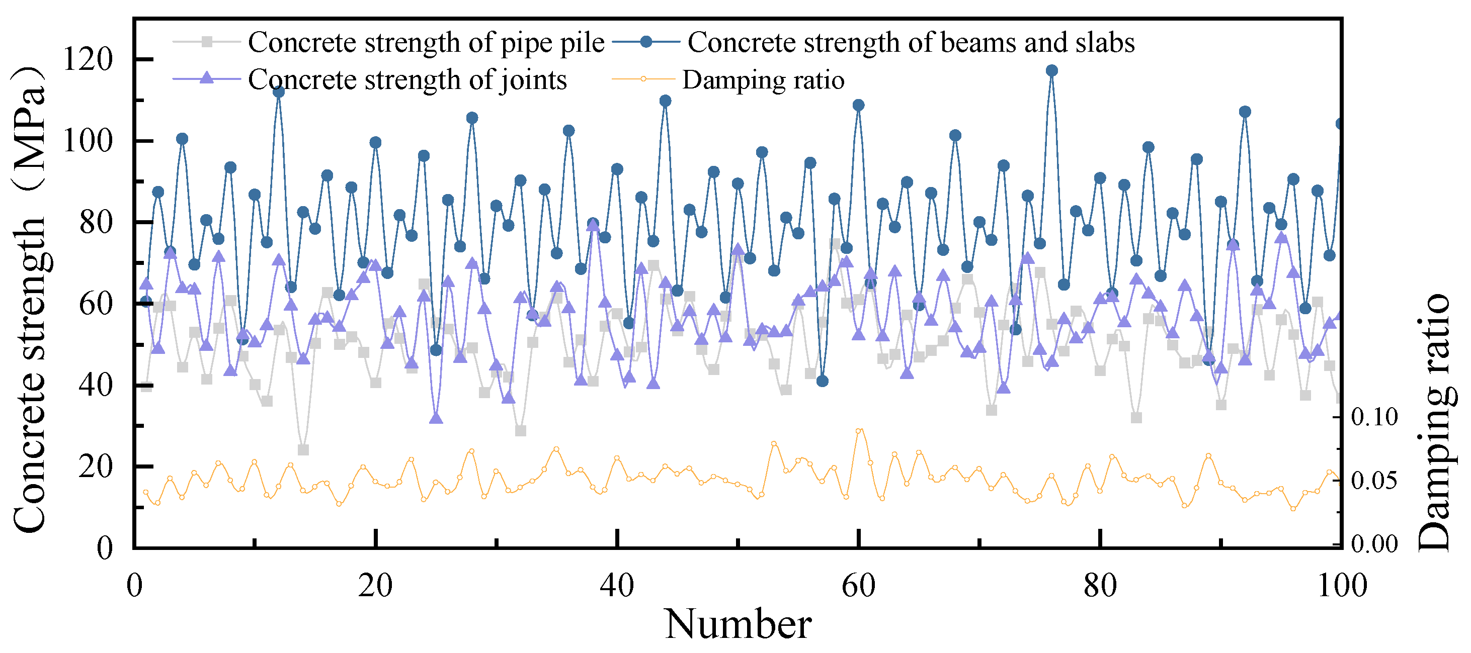
3.1. Random Structure Analysis Model of Pile–Plate Structure

The standard longitudinal length of the pile–plate structure for this highway is 8 × 8 m per unit, with a total length of 64 m. It adopts a double-sided, two-lane form, with a single lane full width of 13.82 m. It is composed of six precast T-beams made of reinforced concrete and five longitudinally cast wet joints with a width of 0.453 m. The lower pile is rigidly connected to the upper structure, with self-restoring nodes providing intermediate connections, which together with the core-filling concrete inside the pile form a load-bearing structure. The structural diagrams are shown in (a), (b), and (c) in Figure 1, while (d) shows the form of the self-restoring node structure. In the self-restoring node structure of the pile–plate structure, the steel pipe-filled fixed pile is connected to the upper beam–plate, and a prestressed threaded steel bar is designed at the center of the node to enhance its energy consumption capacity. The steel pipe sleeve, as well as the steel hoop that connects it to the lower core-filled concrete, functions to restrain the concrete, improving the strength and reliability of the connection between the pile and beam–plate nodes.

This significantly improves its bearing capacity. Figure 1d shows the detailed structure composition of the node, including beam plates, rubber strips, core-filling concrete materials, outer steel pipes, pile sleeve hoops, corner welds, temporary steel clamps, piles, core-filled concrete support plates, and prestressed threaded steel bars.

To investigate the dynamic response law of random pile–plate structure under strong earthquake action and taking into account the calculation accuracy and speed, the structural finite element model was established by using the fiber beam element of the OpenSees finite element platform. When modeling, considering the complex, nonlinear mechanical behavior of concrete under the action of force, the ConcreteD concrete stochastic constitutive model in the OpenSees material library is selected. Considering the Bauschinger effect and material hardening, the steel 02 steel constitutive model is selected. According to the site type of the pile–plate structure, an El-Centro seismic wave is selected as the input seismic wave, the acceleration amplitude is modulated by 0.4 g, and the input is consistent along the longitudinal bridge direction.

Our team successively employed ANSYS and OpenSees to conduct simulations on the pile–slab structure designed in this study and performed comparative analysis by applying cyclic loading in the form of horizontal displacement, as shown in Figure 2. Simulated vertical loads from the superstructure were applied to the beam ends of the pile–slab structure, and horizontal displacement loads were imposed on control points for regulation. The displacement levels were set at 1/800, 1/500, and 1/250, with six cycles at each level; at 1/150, four cycles; and at 1/100 and 1/80, with two cycles per level. As shown in Figure 1, the shapes and trends of the hysteresis curves from the two simulations are consistent, with the maximum difference in hysteresis loop area being 0.55%, all less than 1%. The results indicate that the curve fitting between the two is highly accurate, thus validating the reliability of the nonlinear analysis model for pile–slab structures based on OpenSees.

The pile–slab structure was modeled in ANSYS, with the initial model established using Space Claim. The core concrete at the pile–slab node connections uses vibration-mixed steel fiber-reinforced concrete, with a matrix strength of CF40 and a steel fiber volume fraction of 2%, while the remaining parts use C50 concrete. The pile–slab structure employs a separated assembly of pipe piles and precast beams and slabs, with all solid contacts being face-to-face bonded contacts of type conta174, defining that no relative separation or sliding occurs between faces. Reinforcing bars and concrete are connected via coupled nodes, with the specific implementation achieved through the pinball radius in the bonded contact and without considering relative sliding between the reinforcing bar and concrete elements. Steel sleeves are used to protect the nodal concrete, with the sleeve modeled as shell elements and a thickness of 0.05 m. The upper part of the pipe pile is connected to the core concrete, while the lower part is a hollow pipe pile, and during load application, the bottom of the pipe pile is supported by a fixed support. The pile–slab structure was modeled in OpenSees using fiber beam elements. During modeling, the complex, nonlinear mechanical behavior of concrete under load was considered, with the concrete material modeled using Concrete01 based on the Kent–Park modified model, as well as the Mander constitutive model considering the confinement effect of stirrups on the core concrete. The reinforcing bars consider the Bauschinger effect and material hardening issues, using the constitutive model Steel02 that accounts for fatigue effects. The main body of the model uses fiber beam elements, divided into precast beams, nodes, core concrete, steel sleeves, prestressed threaded rebar, rebar cages, and the underlying pipe piles, with the rendered image of the node model shown below. Zero-length elements are used to simulate the self-centering nodes. A rigid element is placed inside the precast beam and slab holes, with its length set to the height of the self-centering node. The nodes at both ends of the element are connected to the nodes at the corresponding positions on the foundation through zero-length elements. Nonlinear properties are then reflected by assigning material attributes.

Utilizing the Pushover analysis method, a maximum lateral linear displacement of 5 cm was applied to the pile–slab structure within 10 s. The resulting equivalent stress contour and plastic strain diagrams are shown in the Figure 3. The relative displacement was obtained by calculating the difference in displacements between the top and bottom surfaces of the nodes. A Pushover curve for the nodes was plotted with relative displacement (m) on the x-axis and shear force (kN) under lateral pushing on the y-axis, as shown in the figure below. Referring to the Code for Seismic Design of Buildings (GB50011-2010) [42], which specifies a limit of 1/30 for the elasto-plastic inter-story drift angle of reinforced concrete frame structures to determine whether the structure has reached a critical state of failure under seismic action, this study sets the top displacement angle of the pier beam, R_μ, as the damage indicator. The damage states of the pile–slab bridge structure under different pier top displacement angle thresholds were determined to provide clear quantitative standards for seismic design and reliability assessment of the structure. I. No-damage state: When the pier top displacement angle is less than 1.0%, the nodes and pipe piles of the pile–slab structure remain in the elastic stage, with no visible cracks in the concrete. The prestressed steel bars and steel fiber-reinforced concrete work well together, and the overall stiffness does not significantly degrade, indicating that the structure remains functional and does not require repair under rare earthquakes. II. When the displacement angle reaches 2.0%, the steel fiber-reinforced concrete in the nodes locally enters the plastic stage due to vibration, with microcracks appearing. However, the outer steel casing and prestressed steel bars still provide effective restraint, and the residual deformation can self-recover. The structural function is essentially intact, and the damage can be restored through local repair. III. Moderate-damage state: After the displacement angle exceeds 3.3%, the core concrete in the nodes cracks and extends, the steel casing undergoes local buckling, and part of the prestressed steel bars yield, with the hysteresis curve showing a significant pinching effect. IV. Severe-damage initiation state: When the displacement angle reaches 4.0%, the plastic hinges in the pile–slab connection nodes are fully formed, the steel fiber-reinforced concrete is crushed and spalls off, the outer steel casing deforms significantly, the structural stiffness drops sharply, and the repair cost is high and technically complex. V. Collapse-warning state: After the displacement angle exceeds 7.0%, the pile–slab structure as a whole forms a mechanism, with the bottom of the pipe piles breaking, the prestressed steel bars breaking, and the core concrete completely failing, resulting in the loss of load-bearing capacity.

3.2. Calculation of Seismic Reliability of Random Structure of Pile–Plate Structure

In order to investigate the dynamic response characteristics of pile–plate random structures under strong earthquake loads while considering both the accuracy and speed of calculations, a finite element model of the structure was established using fiber beam elements in the OpenSees finite element platform. During modeling, the complex, nonlinear mechanical behavior of concrete under stress was considered, and the Concrete01 concrete stochastic constitutive model in the OpenSees material library was selected. The Steel02 steel constitutive model was used to consider Bauschinger effect and material hardening issues for steel bars under stress. Four structural parameters, including the compressive strength of pipe-pile concrete, beam–plate concrete, and joint concrete and the damping ratio ζ of the structure, were selected as basic random variables, and their mean values and coefficients of variation were determined. The node-filled core concrete was made of vibratory-mixed steel fiber concrete with a matrix strength of CF40 and a steel fiber volume rate of 2%. Based on the test data and statistical analysis data, the mean value of its cubic compressive standard strength was determined to be 56.5 MPa, and this random variable conformed to a normal distribution with a coefficient of variation of 0.15. The statistical information and distribution types of the above random variables are shown in

Table 1. Structural random variables.

	Random Variables	Mean	Coefficient of Variation	Distribution Type
Concrete strength of pipe pile	fr,v1 (C60)	60 MPa	$0.17$	Normal distribution
Concrete strength of beams and slabs	fr,v2 (C50)	50 MPa	$0.17$	Normal distribution
Concrete strength of joints	fr,v3 (CF40)	56.5 MPa	$0.15$	Normal distribution
Damping ratio	ζ	$0.05$	$0.2$	Lognormal distribution

and Figure 4, and all variables were assumed to be statistically independent.

The main process of seismic reliability analysis of pile–plate random structures using the probability density evolution method is as follows: first, the basic random variables of the structure are determined. Based on the GF deviation point selection method [43], 100 sets of discrete representative points for the structural random parameters are generated, and the assigned probability for each group of point sets is determined to generate a sample set of pile–plate random structures. The point selection method can ensure the uniformity and accuracy of the selected point set, thereby effectively reflecting the distribution characteristics of random variables. Then, the selected earthquake waves are input to obtain the seismic response results of the pile–plate random structure samples, and the Newmark-$\beta$ is used in the implicit algorithm to solve the motion equation of the structure under deterministic earthquake excitation. After that, the TVD difference algorithm is used to solve the probability density evolution equation, which can obtain the probability density evolution information of the structural response in the solving time interval. Finally, based on the first surpassing failure criterion, the seismic reliability of the pile–plate random structure is calculated by absorbing boundary conditions with different threshold values. The specific solution process is shown in Figure 5.

In order to obtain the complete probability density evolution information of pile–plate structures under seismic action, the response of the pile–plate structure under strong earthquake action was analyzed, and the improvement of the seismic reliability of the pile–plate structure by self-resetting nodes was explored. After generating all pile–plate structure samples using the GF bias method, El-Centro earthquake waves with the same type II site as the pile–plate structure were used, and the acceleration modulation value was increased to 0.4 g, inputting them simultaneously along the transverse and longitudinal directions of the pile–plate structure. The acceleration time history of earthquake motion and the corresponding response spectrum are shown in Figure 6.

Starting from the perspective of deformation angles, the displacement angles of edge-span beams and columns of pile–plate structures are selected to analyze the stochastic evolution process of the structure. Considering these factors, such as the study’s objectives, available computational resources, and the desired level of result confidence, 100 seismic response analyses were performed on the generated random structural samples, and the time history curve of R_μ, which represents the displacement angle of the top of edge-span beams and columns of pile–plate structures, as shown in Figure 7. According to Figure 7, due to the stochasticity of structural parameters, under the same seismic action, the structural responses of pile–plate structures also exhibit randomness, manifested as fluctuations within the limit range of −3% to 3% for R_μ. The obtained structural response information was combined with given probabilities to calculate the statistical mean and standard deviation of structural R_μ responses, as shown in Figure 8. It can be seen that due to the influence of the stochasticity of structural parameters, the seismic response of the structure has variability, further illustrating the importance of considering the stochasticity of structural parameters in seismic response analysis of pile–plate structures.

By using the TVD differencing algorithm, joint Equations (1) and (2) were used to solve the probability density evolution equation of R_μ for the pile–plate structure. Based on the results obtained from the probability density evolution equation, surface plots, contour plots, and probability density function curves of R_μ for typical time periods were drawn, as shown in Figure 9. The undulations of the surface plot in Figure 9a reflect the evolution of the probability density function of the displacement angle of the pile–plate structure with time, while the range of displacement angle also evolves with the loading process of earthquake. The probability density contour map of R_μ, i.e., the contour plot of probability density in Figure 9b, provides a more intuitive representation of the random fluctuations of R_μ over time. By analyzing the probabilistic information on the structural response under seismic action, we can better understand and grasp the variation rule of the displacement angle at the top of the pier over time, which lays the foundation for the reliability analysis of the pile–plate structure. At t = 8.2 s, 11.1 s, and 14.1 s in Figure 9c, the probability density function curves of R_μ are selected, and the differences among the three curves indicate that the range and probability density function of R_μ have also been constantly changing over time under the same seismic action.

All these results indicate that the randomness of material parameters of the pile–plate structure leads to complex random evolution processes in its seismic response. Therefore, when conducting seismic response analysis and seismic reliability research on pile–plate structures, the randomness of structural parameters should be fully considered to make the research results closer to engineering reality. Furthermore, through the probabilistic density evolution method, rich probabilistic information on structural response can be obtained, providing a foundation for studying the nonlinear seismic response rules of pile–plate structures and then carrying out seismic reliability evaluation.

After obtaining the probability density information of R_μ of pile–plate random structure under seismic action, based on the first-exceeding failure criterion and by absorbing boundary conditions of different failure thresholds, the seismic reliability of a pile–plate random structure is calculated, as shown in

Table 2. Seismic reliability of pile–plate structures under different failure thresholds.

Rμ/%	Reliability
3.3	100.00%
2.1	98.05%
2.0	90.17%
1.0	65.26%

. The variation curves of earthquake-proof reliability of pile–plate structure with different thresholds over time are shown in Figure 10.

As shown in Figure 10, the seismic reliability curve of pile–plate structures undergoes a step change over time and eventually stabilizes. Under different failure thresholds, there are significant differences in the seismic reliability of pile–plate structures. When the failure threshold is 1.0%, the seismic reliability of the pile–plate structure is only 65.26%. However, when the failure threshold is set to 3.3%, the seismic reliability of the pile–plate structure reaches 100%, with a difference of 34.74%. Concurrently, this 100% numerical performance also serves as the rationale for conducting a multi-point value analysis of the failure threshold below 3.3% rather than continuing to take values upward.

The failure threshold determined through reliability analysis refers to a single-layer reinforced concrete frame column of steel-reinforced concrete racks, which has the closest structural form to the pile–plate structure specified in the “Code for Seismic Design of Buildings” (GB50011-2010)[42]. The limit value of the inter-story drift angle of ductility-based design, 1/30, for steel-reinforced concrete frame structures is taken as the limit for the beam displacement angle of the edge span of the pile–plate structure when determining its seismic performance under an earthquake with a PGA of 0.4 g, resulting in an earthquake resistance reliability of 100% for this random pile–plate structure. Although there are differences between steel-reinforced concrete frame structures and pile–plate structures, it should be noted that there are some errors in using this failure limit value to assess the reliability of pile–plate structures, and this method provides a new idea for studying the reliability of pile–plate structures.

4. Reliability Analysis of Structures Under Random Earthquake Excitations

According to earthquake disaster statistics, the main reason for building damage and destruction in seismic disasters is the lack of understanding of the seismic performance and dynamic damage mechanism of structures [44,45]. Due to the randomness of earthquake excitation, pile–plate structures will suffer structural damage or collapse under strong seismic action. The location of the damage is uncertain. It is greatly limited to use determinate natural earthquake waves or artificially synthesized earthquake waves for seismic reliability analysis of pile–plate structures, as this cannot fully reflect the structural seismic performance [46]. Therefore, accurately assessing the reliability of pile–plate structures under random seismic action is of great significance for improving their ability to defend against seismic disasters. Based on the established fiber beam element model of pile–plate structures and combining it with a physical model of random ground motion, nonlinear dynamic analysis and seismic reliability analysis of pile–plate structures under random seismic action were carried out using the probability density evolution method in this section.

4.1. Physical Stochastic Function Model of Engineering Ground Shaking

Due to the unpredictability of the time, location, and intensity of earthquakes, it is difficult to describe the randomness of earthquake motion in a specific way. The modeling method of using random earthquake motion based on the viewpoint of physical random systems determines the relevant physical earthquake motion model parameters by statistically analyzing the physical elements that affect the randomness of earthquake motion (propagation path, source characteristics, and site conditions where buildings are located) in order to describe the randomness of earthquake motion, being an effective method for establishing engineering random earthquake motion physical models [47].

The classical power spectrum model describes the second-order statistical characteristics of earthquake motion based on the assumptions of stationarity and ergodicity, but this earthquake motion modeling method has certain limitations. Li J et al. [48] proposed an engineering random earthquake motion physical model but did not conduct in-depth research on the impact of source characteristics, propagation paths, and site conditions where buildings are located on earthquake motion. Ding et al. [49,50,51,52,53] analyzed recorded earthquake motions through the K-means algorithm to obtain the probability density function of basic parameters that affect earthquake motion in the physical modeling of engineering random earthquake motion, further improving the physical modeling of engineering random earthquake motion.

The time course of ground-shaking acceleration can be expressed as follows:

$$a_R\left(t\right)=-{\displaystyle \frac{1}{2\pi }}{\int }_{-\infty }^{+\infty }{A}_R\left({\Theta }_{\alpha },\omega \right)\times \mathit{cos}\left[\omega t+{\Phi }_R\left({\Theta }_{\alpha },\omega \right)\right]d\omega$$

(14)

where $A_R\left({\Theta }_{\alpha },\omega \right)$ is the Fourier amplitude spectrum (see Equation (15)); ${\Phi }_R\left({\Theta }_{\alpha },\omega \right)$ is the Fourier phase spectrum (see Equation (16)); and ${\Theta }_{\alpha }$ is the random parameter vector of ground shaking (see Equation (17)).

$$A_R\left({\Theta }_{\alpha },\omega \right)={\displaystyle \frac{A_0\omega e^{-K\omega R}}{\sqrt{{\omega }^2+{\left(1/\tau \right)}^2}}}\times \sqrt{{\displaystyle \frac{1+4{\xi }_g{\left(\omega /{\omega }_g\right)}^2}{{\left[1-{\left(\omega /{\omega }_g\right)}^2\right]}^2+4{\xi }_g{\left(\omega /{\omega }_g\right)}^2}}}$$

(15)

$${\Phi }_R\left({\Theta }_{\alpha },\omega \right)=\mathit{arctan}\left({\displaystyle \frac{1}{\tau \omega }}\right)-R\cdot \mathit{ln}\left[a\omega +1000b+0.1323\mathit{sin}\left(3.78\omega +c\mathit{cos}\left(d\omega \right)\right)\right]$$

(16)

$${\Theta }_{\alpha }=\left(A_0,\tau ,{\xi }_g,R,a,b,c,d\right)$$

(17)

Here, $A$ is the amplitude factor; $\tau$ is the seismic source coefficient; ${\xi }_g$ is the site equivalent damping; and ${\omega }_g$ is the remarkable periodic circle frequency.

The research results indicate that the statistical analysis of the above four basic physical random variables can quantify the unpredictability of seismic ground motions. The propagation coefficient K and the distance from the epicenter $R$ are deterministic variables, generally selected based on actual engineering conditions. The empirical stochastic parameters $a, b, c \mathrm{a}\mathrm{n}\mathrm{d} d$ describe the propagation path and can be identified through parameter recognition. ${\omega }_g \mathrm{a}\mathrm{n}\mathrm{d} {\xi }_g$ determine the probability distribution based on field testing, thus reducing the variability of random ground motion. This stochastic ground motion physical engineering model can describe the random ground motion sample through probabilistic source parameters. $A$ and $\tau$ both approximately conform to the basic characteristics of the lognormal distribution, and ${\xi }_g$ and ${\omega }_g$ approximately conform to the basic characteristics of the gamma distribution. Based on this physical ground motion model and parameter identification of existing ground motion records, the distribution types and statistical parameters of the four basic random variables of the physical stochastic ground motion model are given in

Table 3. Parameters for physical stochastic ground-shaking model, with values [52].

Physical Random Parameters	Distribution Type	Probability Density Function Parameter Value
$A_0$	Lognormal	Venue type	$\mu$	$\sigma$	$\alpha$
		I	−1.4306	0.9763	0.05
		II	−1.2712	0.8267	0.05
		III	−1.1047	0.7388	0.15
		IV	−0.9280	0.6380	0.25
$\tau$	Lognormal	Venue type	$\mu$	$\sigma$	$\alpha$
		I	−1.3447	1.4724	0.10
		II	−1.2403	1.3436	0.05
		III	−1.1574	1.1341	0.10
		IV	−0.9712	1.0553	0.20
${\xi }_{\mathrm{g}}$	Gamma distribution	Venue type	$k$	$1/\theta$	$\alpha$
		I	3.9368	0.1061	0.05
		II	5.1326	0.0800	0.05
		III	6.1838	0.0689	0.05
		IV	6.4089	0.0658	0.25
${\omega }_{\mathrm{g}}$	Gamma distribution	Venue type	$k$	$1/\theta$	$\alpha$
		I	2.0994	9.9279	0.10
		II	2.2415	7.4136	0.05
		III	2.0866	5.6598	0.25
		IV	1.9401	5.5265	0.20

.

Accordingly, the parameters of the physical stochastic ground-shaking model are used to generate stochastic ground-shaking samples for the stochastic seismic response analysis of pile–plate structures based on the probability density evolution method.

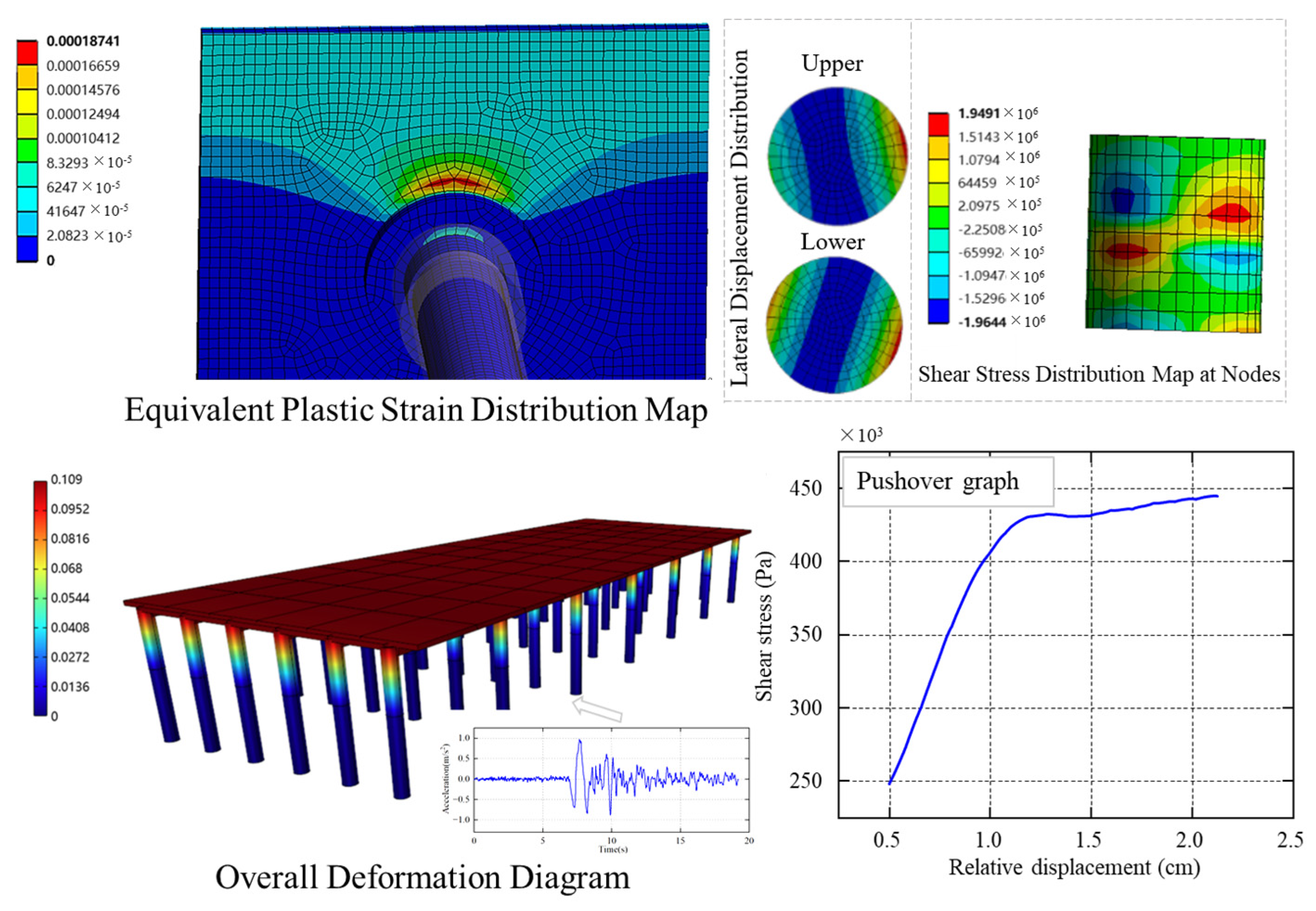
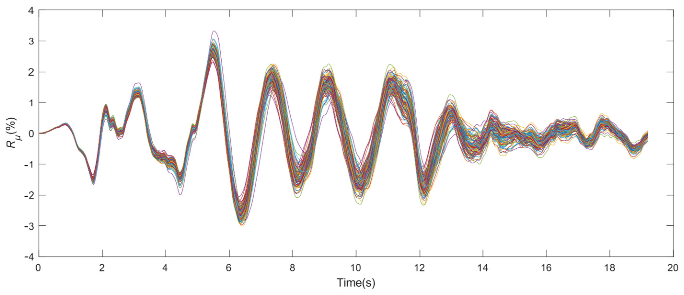
4.2. Stochastic Seismic Response Analysis and Seismic Reliability Assessment of Pile–Plate Structures

Earthquake excitations possess a high level of randomness and uncertainty, making it difficult for the existing scientific technological level to accurately predict seismic motions, which complicates the reliability analysis of pile–plate structures. Therefore, accurately assessing the seismic reliability of pile–plate structures under strong earthquakes is of great significance to improve structural safety. Based on this, nonlinear dynamic analyses of pile–plate structures with either self-centering or conventional rigid connections are carried out under stochastic earthquake excitations to describe the stochastic dynamic response characteristics of pile–plate structures, obtain probability density evolution information of pile–plate structures under stochastic earthquake excitations, and calculate structural dynamic reliability under different failure thresholds.

The process of seismic reliability analysis of pile–plate structures under stochastic earthquakes is shown in Figure 11. A point-set method using GF deviation is used to select representative points with discretization, generating seismic motion samples with assigned probabilities to analyze the seismic responses of pile–plate structures. The implicit Newmark-β method is used to solve the motion equations, calculating the displacement responses of pile–plate structures, followed by solving the probability density evolution equation, obtaining the probability density information of pile–plate structures under stochastic earthquake effects. Overall seismic reliability analyses of pile–plate structures are then conducted by absorbing boundary conditions with different thresholds.

Using the GF bias point selection method and based on the values of the four random seismic physical model parameters for type II sites in Table 3, earthquake motion samples with assigned probabilities were generated by selecting a discrete representative point set of these four random parameters. Figure 12 shows the four typical earthquake acceleration time–history curve samples generated, named a, b, c and d, respectively, all with an amplitude of 0.4 g. Figure 13 shows the corresponding response spectra for these four earthquake acceleration time–history curve samples when the damping coefficient is set to 5%.

By inputting the obtained engineering physics random seismic samples into the pile–plate structure analysis model, the displacement angle time history curve shown in Figure 14 is obtained. It can be seen that due to the coupling amplification effect caused by the nonlinearity of the concrete material and the randomness of the seismic excitation, the displacement response of the pile–plate structure is more stochastic.

By combining the structural response information with assigned probabilities, statistical mean and standard deviation curves of the displacement angle are obtained, as shown in Figure 15. By comparing the statistical mean and standard deviation, it is known that the randomness of earthquake excitation results in more than a five-fold increase in the variability of the displacement angle response [35].

The probability density evolution method is used to analyze the nonlinear dynamic response of pile–plate structures under random seismic action and obtain complete probability information about the structural response over a certain time period. This information is used to describe the overall performance of the structure over a period of time and to apply it to the reliability assessment of the pile–plate structures. By absorbing the boundary conditions of different failure thresholds, the dynamic reliability of the pile–plate structure is calculated.

The finite difference method (TVD) is used to solve the probability density evolution equation, and the relevant probability information of the displacement and angle response is obtained, as shown in Figure 16. It can be seen that the probability density evolution information is similar to the R_μ probability density evolution surface of the pile–plate random structure. Under the random seismic action, the probability density surface and contour map of the pier top displacement and angle also show significant stochastic fluctuations with time extension. However, by comparing the relevant probability information of R_μ under the pile–plate random structure (Figure 9) and the relevant probability information of R_μ under random seismic action on the pile–plate structure (Figure 16), it can be concluded that the stochastic fluctuation effect of seismic response caused by seismic randomness is more significant than that caused by structural parameter randomness, and the distribution of the probability density function is more dispersed.

By incorporating the probability density information of the dynamic response of pile–plate structures and adding absorbing boundary conditions that correspond to failure thresholds, the seismic reliability of the pile–plate structures was calculated, as shown in

Table 4. Seismic reliability of pile-slab structures under stochastic seismic excitation with different failure thresholds.

Rμ/%	Reliability
7.0	98.49%
4.0	96.38%
3.3	92.01%
2.0	83.74%
1.0	56.82%

. The seismic reliability curves under different thresholds are shown in Figure 17.

The seismic dynamic reliability of structures using displacement angles as a limit threshold changes significantly with the modification of failure threshold, and as the displacement angle threshold increases, the seismic dynamic reliability gradually improves over time and ultimately stabilizes. Similarly, an interlayer displacement angle of 1/30 is selected as the limit threshold for the displacement angle failure of the pile–plate structure. The seismic reliability of the pile–plate structure with self- resetting nodes under random seismic excitation with a PGA of 0.4 g is 92.01%, which is 7.99% lower than that of a random structure. Compared to the 100% reliability of the random pile–plate structure, the structure is no longer entirely reliable under the action of random seismic movements. This indicates that the randomness of seismic excitations has a greater impact on the seismic response of the pile–plate structure compared to the randomness of structural parameters.

4.3. Seismic Reliability Analysis of Pile–Plate Structure Considering Parameter–Excitation Composite Randomness

In the previous study, random nonlinear dynamic response analysis and seismic reliability research of pile–plate structures were conducted by separately considering the randomness of structural parameters and seismic excitation. However, in practical situations, both randomness factors often coexist, and when the pile–plate structure enters the nonlinear dynamic response stage under seismic action, the randomness factor often combines with the nonlinear factor, thereby amplifying the dynamic response of the structure. Based on this, considering the above two types of random factors, nonlinear dynamic analysis and seismic reliability research of the pile–plate structure under composite random factors are carried out.

4.3.1. Analysis and Evaluation Method for Composite Random Seismic Response of Pile–Plate Structure

The stochastic seismic response and seismic reliability of pile–plate structures under composite stochastic action are studied and analyzed using the probability density evolution method, and the stochasticity of the structural parameters is noted as:

$$M\ddot{X}\left({\Theta }_1,t\right)+C\dot{X}\left({\Theta }_1,t\right)+KX\left({\Theta }_1,t\right)=\mathrm{I}\mathsf{\Gamma }\left({\Theta }_2,t\right)$$

(18)

or written in the form of the following equation of state:

$$\dot{\mathsf{{\rm Y}}}(\Theta ,t)=\mathrm{A}(\mathsf{{\rm Y}}(\Theta ),t)$$

(19)

The randomness of the excitation is characterized by a specific decomposition algorithm. We consider a real zero-mean process $\{X\left(t\right),0\le t\le T\}$ by introducing the standard set of orthogonal functions:

$${\phi }_j\left(t\right),j=1, 2, \cdots \mathrm{s}.\mathrm{t}. <{\phi }_i,{\phi }_j>={\int }_0^T{\phi }_i(t){\phi }_j(t)dt={\delta }_{ij}$$

(20)

On the interval [0, T], $X\left(t\right)$ can be expanded as:

$$X(\xi ,t)=\sum _{h=1}^{\mathrm{\infty }}{\xi }_h{\phi }_h(t)$$

(21)

${\xi }_h$ can be calculated from Equation (20):

$${\xi }_h={\int }_0^{T}X(\xi ,t){\phi }_k(t)\mathrm{d}t,k=1, 2, \cdots$$

(22)

Equation (21) is usually a finite truncation order, if taken as:

$$X(\xi ,t)=\sum _{h=1}^N{\xi }_h{\phi }_h(t)$$

(23)

Then, the random orthogonal coefficients are defined as $\xi =\{{\xi }_h,h=1, \cdots , N\}$, given its covariance matrix as:

$$C=\left[\begin{array}{cccc}{c}_{11}& c_{12}& \cdots & c_{1N}\\ c_{21}& c_{22}& \cdots & c_{2N}\\ ⋮& ⋮& \ddots & ⋮\\ c_{N1}& c_{N2}& \cdots & c_{NN}\end{array}\right]$$

(24)

where each matrix element satisfies:

$$X{c}_{ij}=\mathbb{E}\left[{\xi }_i{\xi }_j\right]$$

(25)

A decomposition of the random vector yields

$$\xi =\sum _{j=1}^N{\zeta }_j\sqrt{{\lambda }_j}{\psi }_j$$

(26)

where ${\lambda }_j$ is the eigenvalue of the covariance matrix; ${\psi }_j$ is the eigenvector corresponding to the covariance matrix; and ${\zeta }_j$ is the standard random variable.

Substituting Equation (26) into Equation (23) yields:

$$\begin{array}{c}X(\xi ,t)\doteq {\displaystyle \sum _{h=1}^N}{\displaystyle \sum _{j=1}^N}{\zeta }_j\sqrt{{\lambda }_j}{\psi }_{jh}{\phi }_h(t)={\displaystyle \sum _{j=1}^N}{\zeta }_j\sqrt{{\lambda }_j}{f}_j(t)\\ f_j(t)={\displaystyle \sum _{h=1}^N}{\psi }_{jh}{\phi }_h(t)\end{array}$$

(27)

When $N\to \infty$, the above equation is equivalent to the K-L decomposition.

Equation (27) can be modified for a non-zero mean stochastic process as:

$$X(\zeta ,t)=X_0(t)+\sum _{j=1}^{\mathrm{\infty }}{\zeta }_j\sqrt{{\lambda }_j}{f}_j(t)$$

(28)

Therefore, the stochastic process can be represented by a finite random variable $\Theta$. Since the sources of randomness are different, i.e., the source of random variable ${\Theta }_1$ is the random parameters of the structure, which is caused by the properties of concrete materials and their inherent material mechanics characteristics, while the source of random variable ${\Theta }_2$ is the random characteristics of earthquake excitation, generated by complex physical mechanisms. Let $\Theta$ denote the union of ${\Theta }_1$ and ${\Theta }_2$ to expand the probability space; then, partition the extended probability space ${\Omega }_{\theta }$ to solve the above problem.

4.3.2. Composite Random Seismic Reliability Analysis of Pile–Plate Structure

To conduct comparative analysis, the fiber beam element model of the pile–plate structure described in the previous section was adopted, and the analysis was conducted under consistent working conditions. In this study, 100 random samples were selected for analysis, but the basic random variables of the structure became eight-dimensional, including four structural random parameters: the compressive strength of concrete for the pile, beam, and slab, the compressive strength of concrete for nodes, and the structural damping ratio; the other four were random seismic physical model parameters. By using the GF bias sampling method, the pile–plate structure was obtained under the compound effect of random structural parameters and random seismic excitation. The seismic motion amplitude obtained was adjusted to 0.4 g. Deterministic dynamic response analysis was performed on 100 samples, and the R_μ time history curve obtained is shown in Figure 18. It can be seen that under the case of considering the compound effect of parameters and excitation randomness, the structural response still exhibits a high degree of randomness under earthquake excitation, and as time progresses, some samples produce irrecoverable residual deformation, and the structural response exceeds the displacement response under a single random factor. This indicates that when considering the compound effect of multiple random factors, the original randomness is amplified, the seismic response of the pile–plate structure is significantly enhanced, and substantial randomness accompanies it.

The probability density information of R_μ obtained using the probability density evolution method is shown in Figure 16. Comparing the probability information related to R_μ under the compound random effect and the single random effect (Figure 9, Figure 15 and Figure 19), it can be seen that under the compound random effect, the iso-density lines of R_μ are more irregular, and the probability density information is also more abundant. The differences in the probability density functions obtained under the three random factor conditions indicate the huge variability of the seismic response of the pile–plate structure under a compound random effect. This is due to the fact that when considering the compound effect of parameters and excitation randomness, the multi-mode and multi-modal features of the structure amplify the combined effect of structural randomness, seismic excitation randomness, and material nonlinearity, which enhances the stochastic evolution effect of the seismic response of the pile–plate structure.

The reliability of the seismic resistance of the pile–plate structure under different thresholds is solved using the same solution ideas as before in

Table 5. Seismic reliability of pile–plate structures under different failure threshold conditions.

Rμ/%	Reliability
7.0	98.18%
4.0	93.24%
3.3	86.38%
2.0	71.65%
1.0	36.62%

, and the reliability curves are shown in Figure 20.

It can be seen that under the compound random effect, the range of seismic reliability variation of the pile–plate structure with self-recoverable nodes is between 36.62% and 98.18% at different failure thresholds, which is greater than the seismic reliability of the structure considering a single random factor. This indicates that under the compound random effect, the variability of the seismic response of the structure is stronger.

4.4. Comparative Study of Seismic Reliability of Pile–Plate Structure

The comparison of the seismic reliability of the pile–plate structure under compound randomness and single randomness is shown in Figure 21. The point-line chart shows the differences in reliability between single stochasticity and compound stochasticity at different thresholds. The seismic reliability of pile–slab structures shows significant differences under the influence of various stochastic factors. When the failure threshold is 3.3%, the seismic reliability considering only the stochasticity of structural parameters is 100%, while considering only the stochasticity of seismic excitation reduces it to 92.01%, and under combined stochasticity, it further decreases to 86.38%. This indicates that the influence of material parameter stochasticity on the seismic reliability of pile–slab bridge structures is less than that of seismic excitation stochasticity. Further comparison between the effects of combined stochasticity and single seismic excitation stochasticity shows that when the failure threshold is relatively high (7.0%), the seismic reliability values are 98.18% and 98.49%, respectively, with a difference of only 0.31%. As the threshold decreases, the difference gradually increases, reaching 3.14% at a 4.0% threshold and 5.63% at a 3.3% threshold. When the threshold is reduced to 2.0% and 1.0%, the differences are 12.09% and 20.2%, respectively.

It is evident that in the nonlinear dynamic analysis of structures, the impact of combined stochasticity on structural response is significantly greater than that of a single stochastic factor. Particularly at lower thresholds, the effect of combined stochasticity on reducing reliability is more pronounced. Therefore, in seismic design, it is crucial to attach great importance to the issue of combined stochasticity and fully consider the combined effects of multiple stochastic factors to ensure the safety and reliability of structures.

5. Conclusions

This paper addresses the seismic reliability of highway pile–slab structures by constructing a nonlinear stochastic dynamic model based on the probability density evolution theory, systematically revealing the impact of combined stochasticity on structural dynamic response and reliability. It provides a new method for the seismic optimization design and reliability analysis of highway pile–slab structures, with the main research achievements as follows:

(1) A nonlinear numerical analysis model for pile–slab structures was established. Multi-scale modeling and analysis of pile–slab structures were conducted, including Pushover and cyclic loading analyses, to determine the damage indicators and five stages of damage development for pile–slab bridges, and the top displacement angle of the pier beam at the edge span was proposed as the core damage indicator. Based on the first-passage failure criterion, the sensitivity of reliability to failure thresholds of 7%, 4%, 3.3%, 2%, and 1% was quantified.

(2) The independent effects of structural parameter stochasticity and seismic excitation stochasticity on pile–slab bridge structures were separately analyzed. By establishing a four-dimensional parameter stochastic model, it was found that in the elasto-plastic stage, the coupling of material nonlinearity and parameter stochasticity causes the reliability curve to exhibit a steep drop followed by a gradual stabilization. When the threshold decreases from 3.3% to 1.0%, the reliability drops by 34.74%, highlighting the critical role of construction quality control in nonlinear response. Through 100 sets of four-dimensional, non-stationary seismic motion models, it was found that at a 3.3% threshold, the seismic reliability is 92.01%, which is 7.99% lower than when considering the stochasticity of structural parameters. This indicates that the stochasticity of seismic motion is more significant than that of structural parameters in causing seismic response in pile–slab structures. It was also demonstrated that traditional single-wave analysis underestimates the risk of non-stationarity in seismic motions.

(3) An eight-dimensional combined stochastic space model was developed to achieve efficient coupled solution and seismic reliability analysis of the pile–slab bridge structural system. The generalized probability density evolution equation-driven efficient reliability analysis framework was applied to the fiber beam element model of pile–slab bridges, overcoming the computational bottleneck of the traditional Monte Carlo method in high-dimensional stochastic spaces. When the threshold decreases from 3.3% to 1.0%, the reliability drop under combined stochasticity reaches 35.64%, significantly higher than that of a single factor. This result indicates that under low-threshold conditions, the weakening effect of combined stochasticity on reliability is more pronounced, revealing the necessity of setting dynamic threshold correction factors for rare extreme events in seismic design.

References

1. Stewart, E.A. The 1999 Jl-Jl Earthquake Tiwan—The Investigation into the Damage to Civil Engineering Structures; Japan Society of Civil Engineering: Tokyo, Japan, 1999; Volume 12. [Google Scholar]
2. Wang, X.; Yang, Z.; Yates, J.; Jivkov, A.; Zhang, C. Monte carlo simulations of mesoscale fracture modelling of concrete with random aggregates and pores. Constr. Build. Mater. 2015, 75, 35–45. [Google Scholar] [CrossRef]
3. Unger, J.F.; Eckardt, S. Multiscale modeling of concrete from mesoscale to macroscale. Arch. Comput. Methods Eng. 2011, 18, 341–393. [Google Scholar] [CrossRef]
4. Guan, J.; Yuan, P.; Hu, X.; Qing, L.; Yao, X. Statistical analysis of concrete fracture using normal distribution pertinent to maximum aggregate size. Theor. Appl. Fract. Mech. 2019, 101, 236–253. [Google Scholar] [CrossRef]
5. Ren, Q.W.; Yin, Y.J.; Shen, L. Fractal study of random distribution of concrete aggregates and its effect on damage characteristics. J. Water Resour. 2020, 51, 1267–1277. [Google Scholar]
6. Husek, M.; Kala, J. Material structure generation of concrete and its further usage in numerical simulations. Struct. Eng. Mech. 2018, 68, 335–344. [Google Scholar]
7. Feng, D.C.; Li, J. Stochastic nonlinear behavior of reinforced concrete frames. Ii: Numerical simulation. J. Struct. Eng. 2016, 142, 4015163. [Google Scholar] [CrossRef]
8. Zhang, J.C. Simulation of Concrete Damage Process Considering the Effect of Material Non-Homogeneity; Southeast University: Nanjing, China, 2015. [Google Scholar]
9. Liu, Z.J.; Zheng, L.H.; Ruan, X.X. Reduced-dimensional simulation of ground vibration considering randomness and correlation of site soil parameters. Vib. Shock. 2021, 40, 165–172. [Google Scholar]
10. Zeng, M.H.; Wu, Z.M.; Wang, Y.J. A stochastic model considering heterogeneity and crack propagation in concrete. Constr. Build. Mater. 2020, 254, 119289. [Google Scholar] [CrossRef]
11. Feng, D.C.; Yang, C.D.; Ren, X.D. Multi-scale stochastic damage model for concrete and its application to rc shear wall structure. Eng. Comput. 2018, 35, 2287–2307. [Google Scholar] [CrossRef]
12. Liang, R.J.; Wang, H.; Shen, H.J. Dynamic response analysis of continuous girder bridge with seismic isolation curve considering randomness of ground vibration. J. Vib. Eng. 2020, 33, 834–841. [Google Scholar]
13. Xu, B.; Pang, R.; Zhou, Y. Verification of stochastic seismic analysis method and seismic performance evaluation based on multi-indices for high cfrds. Eng. Geol. 2020, 264, 105412. [Google Scholar] [CrossRef]
14. Kavitha, P.E.; Beena, K.S.; Narayanan, K.P. A review on soil–structure interaction analysis of laterally loaded piles. Innov. Infrastruct. Solut. 2016, 1, 14. [Google Scholar] [CrossRef]
15. Islam, R.; Das Turja, S.; Van Nguyen, D.; Forcellini, D.; Kim, D. Seismic soil-structure interaction in nuclear power plants: An extensive review. Results Eng. 2024, 23, 110783. [Google Scholar] [CrossRef]
16. Liu, J.; Jin, Q.; Dong, Y.; Tian, L.; Wu, Z. Resilience-based seismic safety evaluation of pile-supported overhead transmission lines under depth-varying spatial ground motions. Reliab. Eng. Syst. Saf. 2025, 256, 110783. [Google Scholar] [CrossRef]
17. Pang, R.; Xu, B.; Zhou, Y.; Song, L. Seismic time-history response and system reliability analysis of slopes considering uncertainty of multi-parameters and earthquake excitations. Comput. Geotech. 2021, 136, 104241–104245. [Google Scholar] [CrossRef]
18. Wu, Y.; Mo, H.H.; Yang, C. Study on dynamic performance of a three-dimensional high frame supported u-shaped aqueduct. Eng. Struct. 2006, 28, 372–380. [Google Scholar] [CrossRef]
19. Liang, J.Y.; Wang, H.; Xu, X.Y. Analysis of seismic dynamic properties of ferry structure based on viscoelastic boundary. People’s Yellow River 2020, 42, 81–84, 102. [Google Scholar]
20. Li, J.; Chen, J.B. Probability density evolution equation in stochastic dynamical systems and its research progress. Adv. Mech. 2010, 40, 170–188. [Google Scholar]
21. Liu, Z.J.; Chen, J.B.; Li, J. Probabilistic density evolution method for nonlinear stochastic seismic response of structures. J. Solid Mech. 2009, 30, 489–495. [Google Scholar]
22. Chen, J.B.; Li, J. The extreme value distribution and dynamic reliability analysis of nonlinear structures with uncertain parameters. Struct. Saf. 2007, 29, 77–93. [Google Scholar] [CrossRef]
23. Goller, B.; Pradlwarter, H.J.; Schueller, G.I. Reliability assessment in structural dynamics. J. Sound Vib. 2013, 332, 2488–2499. [Google Scholar] [CrossRef]
24. Su, C.; Xu, R. Time domain solution for dynamic reliability of structural systems under non-stationary random excitation. J. Mech. 2010, 42, 512–520. [Google Scholar]
25. Liu, Z.J.; Li, J. Dynamic Reliability Assessment of Non-Linear Structures Under Earthquake Loads; Science Press: Beijing, China, 2007. [Google Scholar]
26. Chen, J.B.; Li, J. Dynamic reliability analysis of composite random vibration systems. Eng. Mech. 2005, 22, 52–57. [Google Scholar]
27. Li, J.; Chen, J.B. The dimension-reduction strategy via mapping for probability density evolution analysis of nonlinear stochastic systems. Probabilistic Eng. Mech. 2006, 21, 442–453. [Google Scholar] [CrossRef]
28. Li, J. Stochastic Structural Systems—Analysis and Modeling; Science Press: Beijing, China, 1996. [Google Scholar]
29. Li, J.; Chen, J.B. A probabilistic density evolution method for the analysis of dynamic response of stochastic structures. J. Mech. 2003, 35, 437–442. [Google Scholar]
30. Li, J.; Chen, J.B. The probability density evolution method for dynamic response analysis of non-linear stochastic structures. Int. J. Numer. Methods Eng. 2006, 65, 882–903. [Google Scholar] [CrossRef]
31. Li, J.; Chen, J.B. Probabilistic density evolution method for dynamic reliability analysis of stochastic structures. J. Vib. Eng. 2004, 17, 121–125. [Google Scholar]
32. Chen, J.B.; Li, J. Density evolution method for dynamic reliability of nonlinear stochastic structures. J. Mech. 2004, 36, 196–201. [Google Scholar]
33. Chen, J.B.; Li, J. Probability density evolution method for composite random vibration analysis of random structures. Eng. Mech. 2004, 21, 90–95. [Google Scholar]
34. Li, J.; Chen, J.B. The principle of preservation of probability and the generalized density evolution equation. Struct. Saf. 2008, 30, 65–77. [Google Scholar] [CrossRef]
35. Li, J. Progress of research on overall reliability analysis of engineering structures. J. Civ. Eng. 2018, 51, 1–10. [Google Scholar]
36. Li, J.; Chen, J.B.; Fan, W.L. The equivalent extreme-value event and evaluation of the structural system reliability. Struct. Saf. 2007, 29, 112–131. [Google Scholar] [CrossRef]
37. Li, J.; Yan, Q.; Chen, J.B. Stochastic modeling of engineering dynamic excitations for stochastic dynamics of structures. Probabilistic Eng. Mech. 2012, 27, 19–28. [Google Scholar] [CrossRef]
38. Chen, J.B.; Li, J. Development-process-of-nonlinearity-based reliability evaluation of structures. Probabilistic Eng. Mech. 2007, 22, 267–275. [Google Scholar] [CrossRef]
39. Chen, J.B.; Jie, L. A note on the principle of preservation of probability and probability density evolution equation. Probabilistic Eng. Mech. 2009, 24, 51–59. [Google Scholar] [CrossRef]
40. Chen, J.B.; Li, J. Dynamic response and reliability analysis of non-linear stochastic structures. Probabilistic Eng. Mech. 2005, 20, 33–44. [Google Scholar] [CrossRef]
41. Huang, H.; Li, Y.; Li, W. Dynamic reliability analysis of stochastic structures under non-stationary random excitations based on an explicit time-domain method. Struct. Saf. 2023, 101, 102313. [Google Scholar] [CrossRef]
42. Ministry of Housing and Urban-Rural Development of the People’s Republic of China, General Administration of Quality Supervision, Inspection and Quarantine of the People’s Republic of China. Code for Seismic Design of Buildings (GB 50011-2010); China Construction Industry Press: Beijing, China, 2010. [Google Scholar]
43. Chen, J.B.; Yang, J.Y.; Li, J. A GF-discrepancy for point selection in stochastic seismic response analysis of structures with uncertain parameters. Struct. Saf. 2016, 59, 20–31. [Google Scholar] [CrossRef]
44. Villaverde, R. Methods to assess the seismic collapse capacity of building structures: State of the art. J. Struct. Eng. 2007, 133, 57–66. [Google Scholar] [CrossRef]
45. Li, J.L.J.; Zhou, H.Z.H.; Ding, Y.D.Y. Stochastic seismic collapse and reliability assessment of high-rise reinforced concrete structures. Struct. Des. Tall Spéc. Build. 2017, 27, e1417. [Google Scholar] [CrossRef]
46. Zhang, W.; Wang, B.; Xu, J.G.; Huang, L. Reliability analysis of water transfer function of large ferry structure under earthquake. J. Civ. Environ. Eng. 2020, 42, 144–152. [Google Scholar]
47. Chen, J.B.; Li, J. New Advances in Stochastic Vibration Theory and Applications; Tongji University Press: Shanghai, China, 2009. [Google Scholar]
48. Li, J.; Ai, X.Q. Research on physics-based stochastic ground vibration model. Earthq. Eng. Eng. Vibration 2006, 26, 21–26. [Google Scholar]
49. Ding, Y.Q.; Peng, Y.B.; Li, J. A stochastic semi-physical model of seismic ground motions in time domain. J. Earthq. Tsunami 2018, 12, 1012–1033. [Google Scholar] [CrossRef]
50. Ding, Y.Q.; Peng, Y.B.; Li, J. Cluster analysis of earthquake ground-motion records and characteristic period of seismic response spectrum. J. Earthq. Eng. 2020, 24, 1012–1033. [Google Scholar] [CrossRef]
51. Ding, Y.Q.; Li, J. Parameter identification and statistical modeling of physical models of engineering stochastic ground shaking. Chin. Sci. Tech. Sci. 2018, 48, 1422–1432. [Google Scholar]
52. Li, J.; Wang, D. Parameter statistics and testing of physical models of engineering stochastic ground shaking. Earthq. Eng. Eng. Vib. 2013, 33, 81–88. [Google Scholar]
53. Chen, J.B.; Li, J. Stochastic seismic response analysis of structures exhibiting high nonlinearity. Comput. Struct. 2010, 88, 395–412. [Google Scholar] [CrossRef]
Figure 1. Structure diagram.
Infrastructures 10 00131 g001
Figure 2. Multi-scale model and fiber beam element model.
Infrastructures 10 00131 g002
Figure 3. Pushover testing of pile–plate–node model.
Infrastructures 10 00131 g003
Figure 4. Four-dimensional random variables of the structure.
Infrastructures 10 00131 g004
Figure 5. Seismic functional reliability analysis process for pile–plate random structures.
Infrastructures 10 00131 g005
Figure 6. Earthquake acceleration time interval and acceleration response spectrum.
Infrastructures 10 00131 g006
Figure 7. Time course curve of the displacement angle of the top of the pier of the structure under the action of earthquake.
Infrastructures 10 00131 g007
Figure 8. Statistical mean and standard deviation of structural displacement angle.
Infrastructures 10 00131 g008
Figure 9. Information on the probability of seismic action Rμ for pile–plate random structures.
Infrastructures 10 00131 g009
Figure 10. Random structural seismic reliability curve.
Infrastructures 10 00131 g010
Figure 11. Seismic reliability analysis process of pile–plate structure with random seismic excitation.
Infrastructures 10 00131 g011
Figure 12. Typical ground-shaking acceleration time scale (0.4 g).
Infrastructures 10 00131 g012
Figure 13. Typical ground vibration acceleration response spectrum (0.4 g).
Infrastructures 10 00131 g013
Figure 14. Time course curve of displacement angle at the top of pier under 0.4 g random earthquake.
Infrastructures 10 00131 g014
Figure 15. Statistical mean and standard deviation of pier top displacement angle under 0.4 g random earthquake.
Infrastructures 10 00131 g015
Figure 16. Probabilistic information of Rμ under random seismic action of pile–plate structures.
Infrastructures 10 00131 g016
Figure 17. Seismic reliability of pile–plate structures.
Infrastructures 10 00131 g017
Figure 18. Time course curve of displacement angle of pier top of pile–plate structure under compound random action.
Infrastructures 10 00131 g018
Figure 19. Probabilistic information of pile–plate structure Rμ under composite random action.
Infrastructures 10 00131 g019
Figure 20. Seismic reliability curve of pile–plate structure.
Infrastructures 10 00131 g020
Figure 21. Comparison of seismic reliability of pile–plate structures.
Infrastructures 10 00131 g021