Cellular Automata for Optimization of Traffic Emission and Flow Dynamics in Two-Route Systems Using Feedback Information

Abstract

Managing emissions and congestion in urban transportation systems is a growing challenge, particularly when traffic dynamics are influenced by real-time conditions and infrastructure constraints. This study addresses this issue by proposing a cellular automata-based model to analyze traffic emissions and flow dynamics in two-route traffic systems under one-directional flow conditions, incorporating various real-time information feedback strategies. Unlike previous studies, the proposed model integrates key components of urban infrastructure, such as lane-changing dynamics, traffic signalization, and vehicle-type heterogeneity, along with operational factors including entry rates, exit probabilities, and the number of waiting vehicles. The model aims to fill a gap in existing emission studies by capturing the dynamics of heterogeneous, multi-lane systems with integrated feedback mechanisms. These considerations provide valuable insights into traffic management and emission mitigation strategies. The analysis reveals that prioritizing information feedback from the system entrance, rather than relying on feedback from the entire system, more effectively reduces traffic emissions. Additionally, the Vehicle Number Feedback Strategy (VNFS) proved to be the most effective, reducing the number of waiting vehicles and consequently lowering CO₂ emissions. Furthermore, simulation results indicate that for entry rate values below approximately 0.4, asymmetrical lane-changing generates higher emissions, whereas symmetrical lane-changing yields elevated emissions when entry rate surpasses this threshold. Overall, this research contributes to advancing the understanding of traffic management strategies and offers actionable insights for emissions mitigation in two-route systems, with potential applications in intelligent transportation infrastructure.

1. Introduction

In recent decades, the societal impact of vehicular traffic has become increasingly evident, marked by congestion, accidents, and air pollution [1]. According to the National Research Council, vehicular emissions are the primary source of greenhouse gases, comprising 45% of US air pollutants [2]. These emissions, including carbon dioxide (CO₂), particulate matter (PM), volatile organic compounds (VOCs), nitrogen oxides (NOx), carbon monoxide (CO), and hydrocarbons (HC), pose environmental and health risks. Hoek et al. [3] found that living near a major road increases cardiopulmonary mortality rates due to particle pollution. Other studies show that high CO₂ exposure harms health, affecting inflammation and cognitive abilities such as problem-solving and decision-making [4,5,6]. Moreover, vehicle emissions also contribute to global warming, smog, and acid rain [7]. Due to these concerns, the EU targets an 80–90% reduction in emissions by 2050, aligning with global efforts [8,9]. These challenges demand integrated strategies that consider not only vehicle behavior but also the design and management of urban infrastructure [10].

Vehicular emissions are closely linked to traffic congestion, especially in urban areas, where interruptions such as traffic lights and speed bumps disrupt traffic flow [11,12]. Thus, driver behavior significantly affects emissions by influencing the acceleration patterns. Studies have shown a correlation between driving behavior and emissions [13]. For instance, De Vlieger et al. [14,15] found that aggressive driving increases fuel consumption by 40% and emissions by 8 times, along with higher levels of VOCs and NO. In response to these challenges, technologies like Intelligent Transportation Systems (ITS) have been proposed to improve traffic management, enhancing efficiency, eco-friendliness, and safety [16,17,18]. As these systems expand, studies show that automation affects traffic dynamics, highlighting the need to address both vehicle behavior and infrastructure design [19,20].

Since the 1990s, Cellular Automata (CA) has been recognized as a key dynamic model for simulating complex systems, valued for its simplicity and efficacy. Researchers from diverse fields, including physics and mathematics, have developed numerous models to tackle the challenges linked to vehicular traffic. Specifically in traffic research, CA models discretize space, time, and vehicle speeds, updating the state of each road cell according to predefined rules. This dynamic process facilitates the exploration of various traffic issues [21,22,23,24,25,26,27]. Several models have been developed to characterize real-world traffic emissions [28,29]. Macroscopic models, which are based on average speed, have been utilized for many years to investigate vehicle emissions [30]. Nevertheless, these models often neglect instantaneous speed fluctuations, which significantly impact real traffic emissions. Consequently, significant efforts have been dedicated to addressing this issue, considering speed fluctuations to calculate emissions in real-time [31,32,33].

Within the CA framework, Yang et al. [34] investigated vehicle emissions and fuel consumption using three different models. They found that these models’ efficiency strongly depends on the traffic density.

Using the Kerner–Klenov–Wolf three-phase cellular automaton traffic model, Xue et al. analyzed fuel consumption for vehicles on one-way lanes under open boundary conditions [35]. The simulation results show that the maximum current (MC) and congested phase have the highest fuel consumption. Synchronized flow (SF) consumes more fuel than free flow but less than MC and congested phase.

Pan et al. [36] studied the effects of various parameters’ effects on fuel consumption and PM emissions in a single lane under open and periodic boundary conditions, including speed limit, entry, and extraction rates. They found that the extraction rate had a more significant overall impact than the entry rate on all the traffic characteristics. Xue et al. [37] analyzed the emissions of CO₂, PM, NOx, and VOC under mixed traffic conditions. Their findings indicated that increasing the mixing ratio leads to higher traffic emissions. In addition, emissions are significantly affected by the maximum speed of shorter vehicles; as the maximum speed of these vehicles increases, so does the magnitude of emissions.

Urban traffic emissions have also been a subject of study. Marzoug et al. [38] analyzed traffic emissions at a signalized intersection, with the study proposing two strategies to reduce vehicle emissions based on traffic density. These strategies have the potential to improve mean speed across all traffic states. Lakouari et al. [39] investigated traffic emissions at a roundabout. They found that CO₂ emissions can be significantly affected even with a few vehicles disregarding the entrance rules to the circulating lane of the roundabout. Additionally, it is observed that variations in the number of traffic signals and cycle times both play crucial roles in influencing CO₂ emissions. Pérez et al. [12] analyzed the vehicle–pedestrian interactions at two kinds of crosswalk systems, namely, raised and zebra, and their impact on CO₂ emissions. They found that raised crosswalks have a milder impact on CO₂ emissions and energy dissipation as they promote traffic calming.

Information is crucial in socio-economic systems, including ITS. Thus, real-time feedback on traffic conditions notably impacts traffic dynamics by reducing travel time and preventing incidents. In this sense, Wahle et al. [40] analyzed traffic flow in route choice, while Dong et al. [41] studied prediction feedback on multi-route traffic flow. Recent studies even have proposed feedback strategies for two-route scenarios [42,43,44,45,46,47].

Studies focusing on a two-route scenario with two exits show that the Mean Velocity Feedback Strategy (MVFS) outperforms the Travel Time Feedback Strategy [46]. Wang et al. [47] demonstrated that Congestion Coefficient Feedback Strategy (CCFS) is more effective than Mean Velocity Feedback Strategy (MVFS) due to the braking probability of the Nagel–Schreckenberg (NaSch) model [48], which results in a fragile speed stability. In a previous study, we introduced a new strategy called the Accident Coefficient Feedback Strategy to reduce accidents and improve the traffic flow [49]. Wu et al. [50] proposed the Ant Pheromone Route Guidance Strategy, where vehicles are analogized to ants, and their traffic information is compared to ant pheromones.

While extensive research has been conducted on the traffic flow characteristics in two-route choice scenarios utilizing feedback strategies, limited investigation has been conducted into their impact on traffic emissions.

Cui et al. [51] studied the impact of different route guidance strategies on traffic emissions. They found that MVFS and CCFS were the best strategies to reduce traffic emissions and enhance traffic flow efficiency. Alam et al. [52] showed that route selection based on air pollution dose correlates with travel time duration, traffic congestion levels, and various other factors that influence emissions dispersion without necessarily affecting the emission rate or total quantity. Furthermore, the effect of real-time information in a two-route scenario on energy consumption was analyzed by Chen et al. [53]. Their findings indicated that feedback strategies have the potential to enhance traffic efficiency and lower energy consumption. As well as acquiring real-time information, it is important to understand how traffic parameters, such as traffic lights, density, heterogeneity, lane-changing processes, driver behavior, etc., influence traffic dynamics.

As single-lane roads become increasingly rare in real traffic scenarios, with most roads being multi-lane, the study of the lane-changing process becomes imperative. Within this framework, Rickert et al. [54] introduced a series of rules to characterize lane-changing. Subsequently, using CA, Chowdhury et al. [55] developed a symmetric/asymmetric two-lane model to examine lane-changing effects. This model has been extensively applied in the analysis of various traffic scenarios [56,57,58,59]. Lane-changing significantly influences traffic characteristics [60] and is considered a critical factor in causing highway congestion [61,62] and reducing road safety [11,63,64]. Furthermore, it is essential to recognize that heterogeneity plays a pivotal role in understanding complex systems [65]. Its importance is particularly observed in vehicular traffic [38,66,67], where heterogeneity encompasses diverse driver behaviors, vehicle types, and road conditions. These factors can lead to intricate and sometimes unpredictable interactions, making it crucial for effective traffic management and modeling.

Despite its importance, traffic emissions in a two-route scenario with information feedback strategies have been largely overlooked. A literature review indicates that only one study [51] has explored this impact. Nevertheless, owing to its novelty, both this study and much of the existing research exhibit significant limitations. For instance, single-lane roads were prioritized over multi-lane roads, as the latter involves lane-changing, which substantially influences traffic dynamics. Traffic was treated as homogeneous, considering only one vehicle type, resulting in a uniform emission rate that diverges from reality. Furthermore, each iteration involved a vehicle attempting to enter the system with an entry rate of 1, overlooking intermediate and low densities, despite traffic demand varying significantly depending on factors such as time of day and day of the week. Additionally, the extraction rate was assumed to be 1, neglecting the dependency of this probability on the traffic state of other connected roads. Moreover, the exclusion of vehicles unable to enter the system at the entrance occludes the real-world scenario where such vehicles are queued, resulting in unaccounted emissions. Finally, the two-route scenario is often modeled without considering traffic lights, despite their common presence in urban areas and crucial role in traffic control.

Overall, there is a significant gap in traffic emission modeling within a two-route scenario that incorporate information feedback strategies, particularly regarding heterogeneous, multi-lane configurations. This paper addresses these limitations, through a cellular automata model that, by isolating key traffic dynamics in a one-directional system as a controlled baseline, integrates multiple realistic features such as lane-changing, vehicle-type heterogeneity, and signal control. The one-directional assumption, while simplified, serves as a foundational case for isolating traffic control effects before extending to bidirectional or networked contexts. Moreover, the broader implications of this study extend to autonomous and connected vehicle systems, fostering communication among vehicles and enabling informed lane-changing decisions based on traffic conditions. Ultimately, this study provides insights for the design of intelligent traffic infrastructure and contributes to advancing sustainable transportation solutions. The insights gained can guide the design and planning of traffic infrastructure under emission-aware smart city policies.

2. Materials and Methods

The model in this paper considers three main aspects: the method for vehicle entrance, which includes heterogeneity of traffic and feedback strategies; vehicle movement, encompassing both longitudinal and horizontal movement (lane-changing); and traffic emissions.

2.1. Heterogeneity of Traffic and Feedback Strategies

In this study, the traffic is heterogenous, comprising two vehicle kinds characterized by their maximum velocities: slow ($v_{smax}$) and fast ($v_{fmax}$); and their proportions are represented by $F_S$ and $F_F$, respectively ($F_S=1-F_F$).

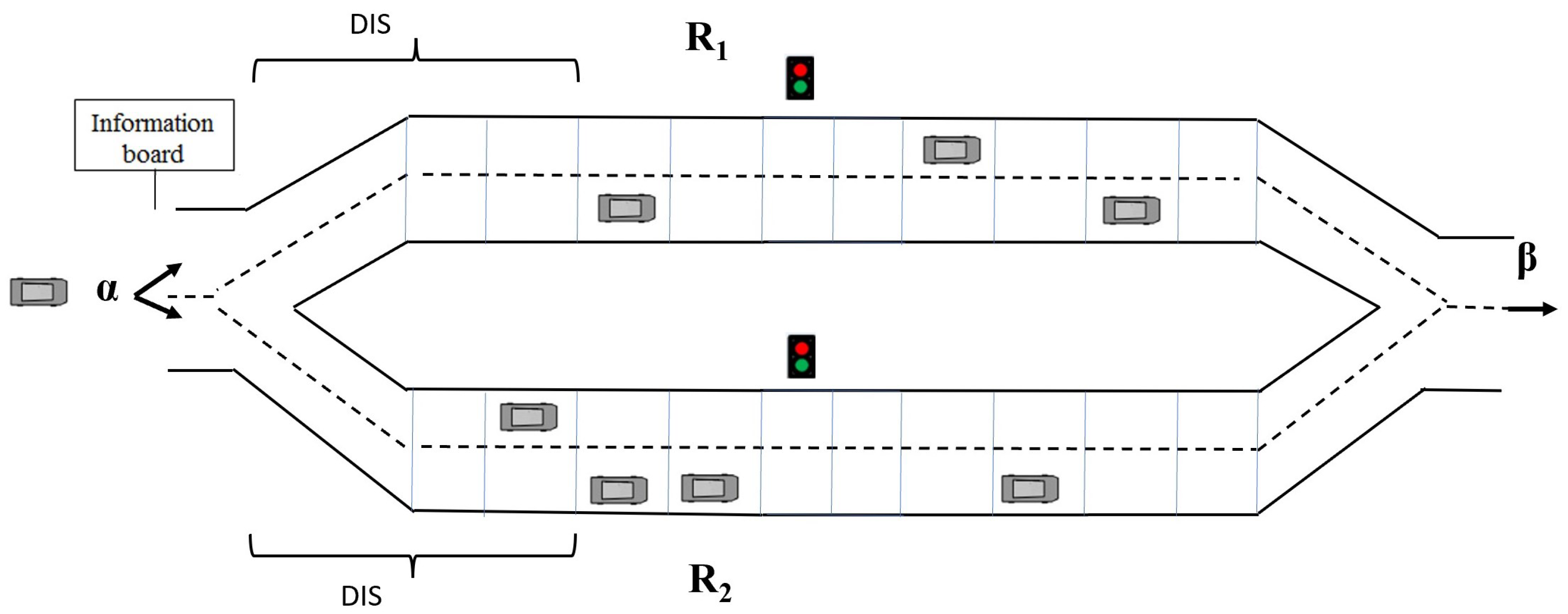
We consider a two-route scenario with one entrance, as shown in Figure 1. Vehicles enter the traffic system (road $R_1$ or road $R_2$) with an entry rate $\alpha$ and exit it with an extraction rate $\beta$. At the entrance, vehicles exhibit a preference. Fast vehicles prioritize the first site of the left lane. If it is occupied, they choose the first site of the right lane. Conversely, slow vehicles prioritize the first site of the right lane. If it is occupied, they choose the first site of the left lane. If the target site is occupied, the vehicle waits for the next iteration before entering the system.

At the entrance, a traffic control center guides drivers to select a route ($R_1$ or $R_2$) based on the utilized information feedback strategy, and then they choose the left or right lane, as explained above. In this context, there are two kinds of drivers: dynamic and static. Dynamic drivers use the information feedback for decision-making, whereas static ones randomly select a route without considering the information feedback. The fractions of dynamic and static drivers are designated as $S_{dyn}$ and 1-$S_{dyn}$, respectively.

Initially, both routes are empty, and the feedback strategy is identical. In the following, we describe the three feedback strategies used in this paper:

• Mean Velocity Feedback Strategy (MVFS): At each iteration, the traffic control center receives the vehicles’ velocity. Subsequently, it calculates and displays the mean velocity within a distance $DIS$ from the entrance (see Figure 1) in each route on the board. At the entrance, arriving drivers select the route with the highest mean velocity. MVFS is considered as one of the most studied strategies [46,50,51].
• Vehicle Number Feedback Strategy (VNFS): This strategy displays the total number of vehicles within a distance $DIS$ from the entrance on each route at every time step. The traffic control center collects and presents this data on the information board. Then, arriving drivers at the entrance choose the route with the fewest vehicles.
• Congestion Coefficient Feedback Strategy (CCFS): It indicates traffic congestion on each route. Each vehicle sends its position to the traffic control center in this scenario. Subsequently, the center calculates and displays the congestion coefficient (CC) within a distance $DIS$ from the entrance in each route, guiding dynamic drivers at the entrance to select the route with the lowest CC. It is calculated using the following formula [47]:

  $$CC=\sum _{i=1}^m{n}_i^w,$$

  (1)

where $CC$ is the congestion coefficient; $n_i$ represents the vehicle number within the ith congestion cluster, where vehicles are closely spaced with no gap between any two of them; w is the weight of each cluster ($w=2$); and m denotes the number of clusters on the route. Numerous other strategies for creating indicators to depict congestion rely on this approach [43,44,45].

2.2. Longitudinal and Horizontal Movement

The system is a two-route scenario, where each route consists of two lanes, and each lane is divided into cells of identical size, each measuring 7.5 m. These cells can either be empty or occupied by a single vehicle (Figure 1). The speed of vehicles can only take integer values: $0,1,\dots ,v_{max}$, where $v_{max}$ is the maximum speed. Furthermore, $v_{max}=v_{fmax}$ for fast vehicles and $v_{max}=v_{smax}$ for slow vehicles ($v_{fmax}>v_{smax}$).

After entering the system, vehicles will adhere to the rules of the NaSch model, and the vehicle’s position is updated at discrete time steps based on the following rules applied in parallel (see [48]):

• Acceleration: $v_i(t+1)=min(v_i\left(t\right)+1,v_{max})$;
• Deceleration: $v_i(t+1)=min(d_i,v_i(t+1))$;
• Randomization: $v_i(t+1)=max(v_i(t+1)-1,0)$, with a probability $P_b$ (braking probability);
• Movement: $x_i(t+1)=x_i\left(t\right)+v_i(t+1)$,

where $d_i$ is the number of empty cells ahead of the vehicle i-th (headway), $v_i$ is the instantaneous speed, and $x_i$ is the vehicle position.

At the end of the system, the two routes intersect, and priority is given equally, with a 0.5 probability for each route. The vehicle without priority decelerates, and its speed becomes $v_i(t+1)=L-x_i\left(t\right)$, where L is the route length. Additionally, if the vehicle’s updated position exceeds the road’s length, the vehicle exits the system with a rate of $\beta$. Otherwise, the vehicle decelerates to maintain its position within the system.

In addition, heterogeneous traffic patterns include a lack of lane discipline and frequent lane changes. In such situations, drivers often switch lanes to maintain high speeds or avoid road incidents.

The rules for lane change can be symmetric or asymmetric, considering either the vehicles or the lanes. In symmetric rules, all vehicles and both lanes are considered equally. However, in asymmetric rules, the lane-changing process depends on the type of vehicle and lane (left or right).

In this paper, lane-changing is allowed if the following conditions are satisfied [55].

Symmetric lane-changing rules:

• $ga{p}_f^c<v_i$;
• $ga{p}_f^o>ga{p}_f^c$;
• The neighboring site in the other lane is empty;
• $v_{i-1}^o<ga{p}_b^o$,

where $ga{p}_f^c$ and $ga{p}_f^o$ are the gaps in front of the vehicle in the current lane and the other lane, respectively; $ga{p}_b^o$ represents the gap between the vehicle in the current lane and the nearest vehicle behind it in the other lane; and $v_{i-1}^o$ is the maximum speed of the vehicle behind the other line.

Asymmetric lane-changing rules:

• Changing from the right to the left:
  Lane-changing rules for slow vehicles remain the same as those of the symmetric model. Nevertheless, for fast vehicles, alongside the symmetric rules, they can switch to the left lane if a slow vehicle is detected within a distance of $v_{fmax}$.
• Changing from the left lane to the right lane:
  In addition to the symmetric rules, a slow vehicle can shift to the right lane if the front gap on the right lane exceeds its current speed. Fast vehicles adopt the same rules as those of slow vehicles, but they do not shift to the right lane if a slow vehicle is detected within a distance of $v_{fmax}$ in the right lane.

Therefore, vehicles can change lanes with a probability $P_{chg}$ if the above rules are met.

2.3. Traffic Emissions

In the existing literature, several traffic emissions models have been proposed. Some rely solely on vehicle power and speed for emission calculation [68,69], while others need numerous vehicle parameters such as the coefficient of drag, engine speed, frontal surface area, and engine displacement [70,71].

In this paper, we used the model proposed by Panis et al. [32] for several reasons. First, this model’s data account for the traffic heterogeneity, including cars, buses, and trucks. Indeed, it enables the calculation of each vehicle’s emissions at each iteration based on both its instantaneous speed and acceleration. Through empirical measurements and non-linear regression techniques, the subsequent general emission function was proposed:

$$E_i\left(t\right)=\max [0,f_1+f_2{v}_i\left(t\right)+f_3{v}_i{\left(t\right)}^2+f_4{a}_i\left(t\right)+f_5{a}_i{\left(t\right)}^2+f_6{v}_i\left(t\right)a_i\left(t\right)],$$

(2)

where $E_i\left(t\right)$, $v_i\left(t\right)$, and $a_i\left(t\right)$ represent the instantaneous CO₂ emission (g/s), the instantaneous speed (m/s), and the instantaneous acceleration (m/s²) of i-th vehicle, respectively. The constants $f_1$ to $f_6$ are determined through regression analysis as detailed in

Table 1. Constants derived from regression analysis for the emission function. [32].

Vehicle Type	${\mathit{f}}_1$	${\mathit{f}}_2$	${\mathit{f}}_3$	${\mathit{f}}_4$	${\mathit{f}}_5$	${\mathit{f}}_6$
Petrol car	$5.53\times {10}^{-1}$	$1.61\times {10}^{-1}$	$-2.89\times {10}^{-3}$	$2.66\times {10}^{-1}$	$5.11\times {10}^{-1}$	$1.83\times {10}^{-1}$
HDV	1.52	1.88	$-6.95\times {10}^{-2}$	4.71	5.88	2.09

. To simplify, we assume that slow vehicles are heavy-duty cars (HDVs, diesel) and fast vehicles are petrol cars.

2.4. Traffic Lights Modeling

Traffic lights are used on both roads $R_1$ and $R_2$ in the middle (Figure 1). This deployment aims to control the incoming flux. The traffic lights can be either symmetric or asymmetric. Symmetric traffic lights have the same period and switch simultaneously on both routes; whereas, in asymmetric traffic lights, when one route has green light, the other route has red light, and vice versa. Here, vehicles approaching the traffic light position in $R_1$ ($R_2$) have priority during a period $T_{g1}$, while the traffic light on $R_2$ ($R_1$) is in the red period $T_r$, and vehicles do not have priority. Afterwards, the light turns red on $R_1$ ($R_2$) and green on $R_2$ ($R_1$) for a period $T_{g2}$.

3. Results

We evaluated the performance of the system under a two-route traffic scenario consisting of two interconnected lanes: a fast lane for priority vehicles and a slow lane for general traffic. The maximum velocities were set to $v_{fmax}=3$ and $v_{smax}=2$, corresponding approximately to 22.5 m/s (81 km/h) and 15 m/s (54 km/h), respectively. The road segment length is $L=1000$ cells, approximating a 7.5 km corridor. This length allows for the observation of large-scale traffic dynamics such as congestion waves and multi-phase flow transitions.

Traffic light cycles were set to $T_{g1}=T_{g2}=T_g=T_r=30$ time-steps, ensuring balanced green and red phases across all intersections. The lane-changing probability is fixed at $P_{\mathrm{chg}}=0.8$, simulating aggressive driver behavior commonly observed under congested urban conditions. Vehicle heterogeneity is modeled through a proportion of fast vehicles $F_f=0.8$, while a braking probability of $P_b=0.1$ introduces stochastic deceleration, capturing driver variability. For all strategies involving feedback-based adaptation (VNFS, MVFS, and CCFS), the dynamic score parameter is set to $S_{\mathrm{dyn}}=1$.

Each simulation was executed for 100,000 time-steps. To ensure the system reaches steady conditions, we compute all reported performance indicators, such as average CO₂ emissions, flow, and delay, based on the last 10,000 time-steps. This procedure is executed across 30 independent simulations, with the aggregated results used to derive mean values, thereby enhancing the statistical confidence of the reported findings.

3.1. Impact of the Feedback Strategy Range on Traffic Emissions

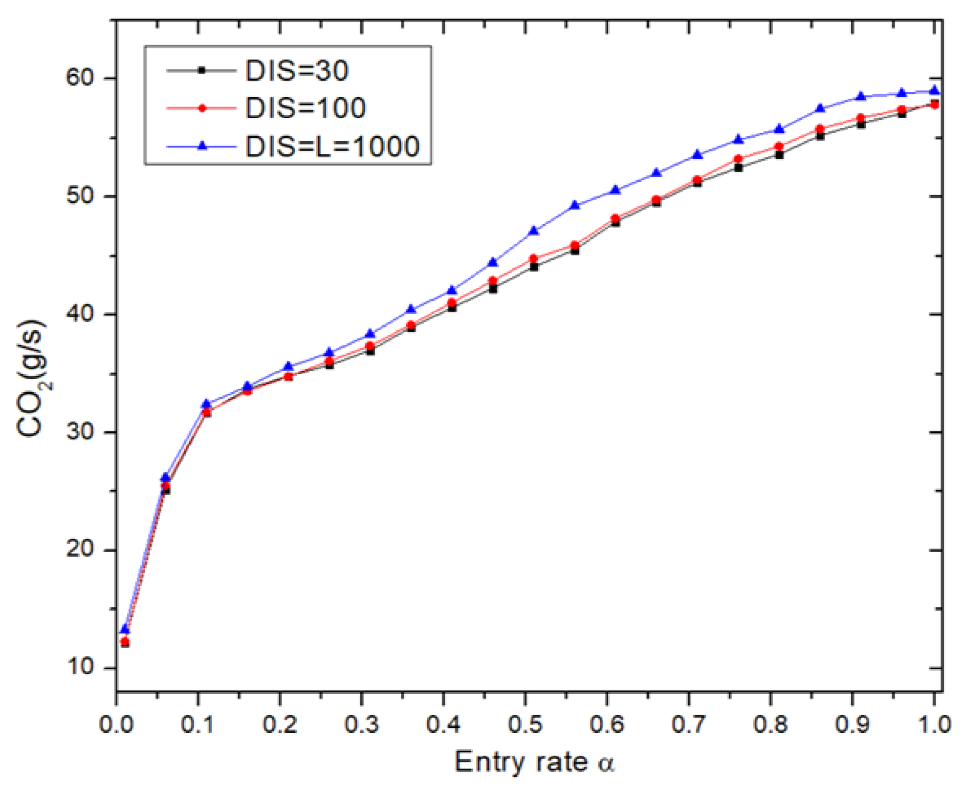
To study the influence of the feedback strategy’s range on traffic emissions, Figure 2 depicts CO₂ emission using VNFS within different distances from the entrance ($DIS$). Across all scenarios, CO₂ emissions exhibit the same qualitative behavior. At low $\alpha$ values, there is no discernible distinction among the various distances. However, as $\alpha$ increases, particularly at higher values, the impact of $DIS$ becomes more evident. Specifically, using a distance of $DIS=30$ results in a reduction of approximately 8% in CO₂ emissions compared to larger feedback ranges. Notably, as $DIS$ decreases, CO₂ emissions also decrease. Thus, the more distant a vehicle is from the entrance, the less its information affects traffic capability. To decrease CO₂ emissions and enhance traffic capacity, the focus should be on providing feedback regarding the condition of the entrance. For the analysis of CO₂ emissions throughout the rest of the paper, $DIS=30$ will be adopted.

3.2. Impact of Traffic Lights on CO₂ Emissions

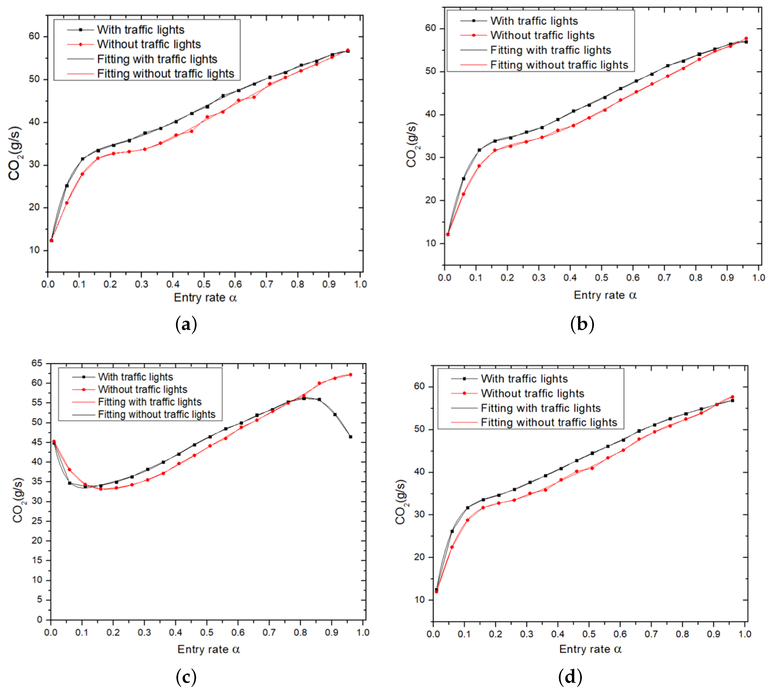
Figure 3 illustrates the variation of CO₂ with respect to $\alpha$, comparing scenarios with symmetric traffic lights and without traffic lights across the four strategies. In the VNFS, CCFS, and $S_{dyn}=0$ (random case), CO₂ emissions increase with increasing $\alpha$. At low $\alpha$ values, CO₂ emissions show a substantial rise until $\alpha =0.16$. Beyond this value, while CO₂ emissions continue to increase, the slope becomes less steep and reaches its maximum at $\alpha$ = 1. In the case with traffic lights, CO₂ emissions exhibit similar qualitative behavior as in the case without traffic lights. However, the inflection point between the two slopes occurs at $\alpha =0.1$; the system without traffic lights shows lower emissions than the system with traffic lights due to the accelerations and decelerations processes at traffic lights.

In the MVFS scenario, CO₂ emissions show a different pattern compared to the three aforementioned strategies. Initially, emissions decrease until $\alpha$ reaches 0.16. Beyond this point, any further increase in $\alpha$ leads to higher emissions. When traffic lights are present, CO₂ emissions follow a similar quantitative behavior and reach the minimum at $\alpha =0.11$. They then increase until $\alpha =0.81$ before decreasing. Notably, the system with traffic lights shows lower emissions at both low and high entry rates. Nevertheless, at intermediate $\alpha$ values, the system without traffic lights exhibits lower emissions.

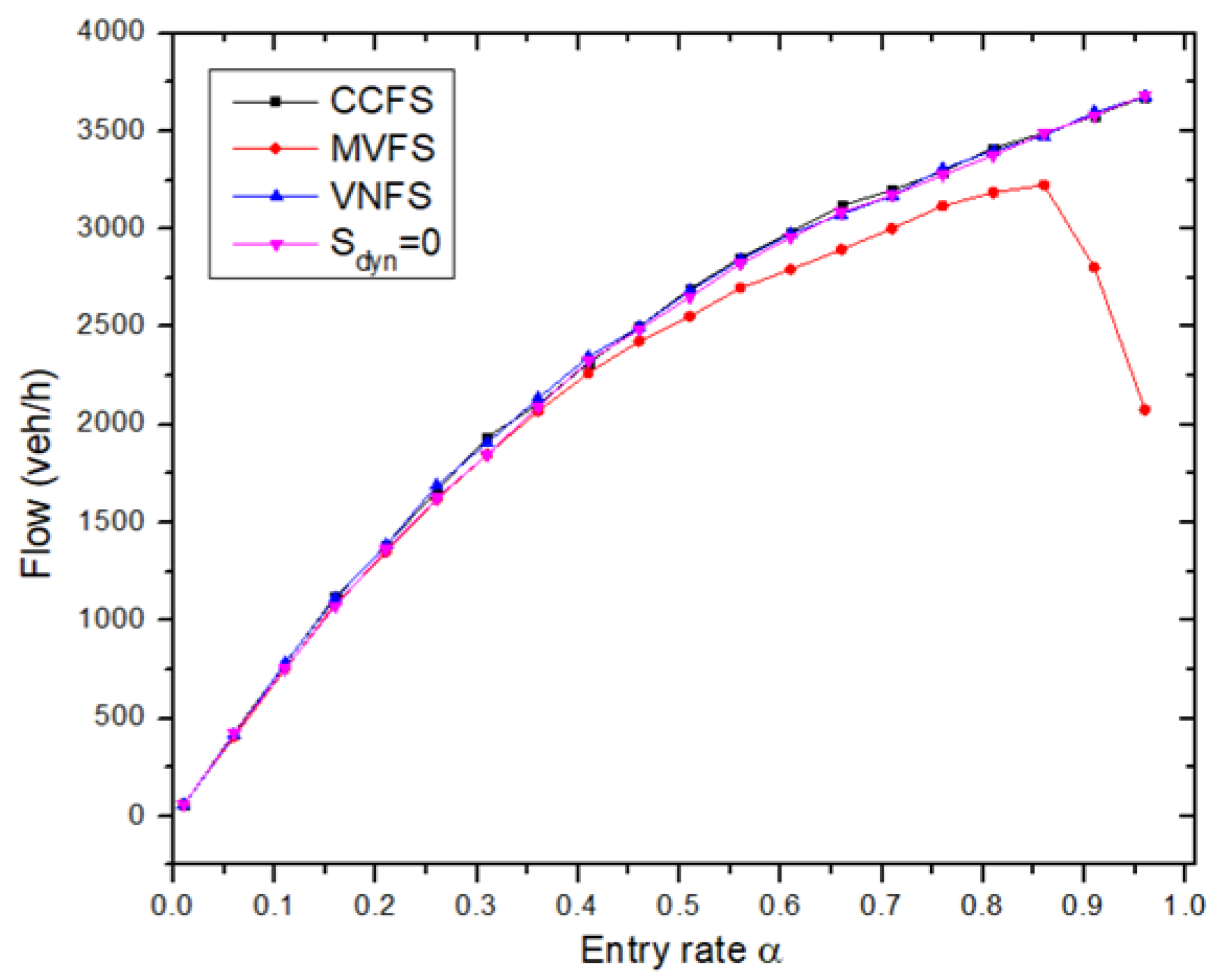
Among the four scenarios, the system with MVFS exhibits higher emissions at low and intermediate entry rates. In contrast, it shows lower emissions at high entry rates. This reduction in emissions is due to the decrease in the traffic flow, as shown in Figure 4. It is worth noting that in all cases, the CO₂ emissions can be expressed as a polynomial of degree 9 in terms of $\alpha$ with the coefficients $a_0,a_1,\dots ,a_9$ (see

Table 2. Coefficients values of the polynomial ($a_0,a_1,\dots ,a_9$).

	VNFS	CCFS	MVFS	${\mathit{S}}_{\mathit{d}\mathit{y}\mathit{n}}=0$
$a_0$	8.341	8.605	48.944	8.082
$a_1$	$4.356\times {10}^2$	$3.{82810}^2$	$-4.{53710}^2$	$4.8\times {10}^2$
$a_2$	$-31.736\times {10}^2$	$-18.131\times {10}^2$	$51.85\times {10}^2$	$-37.607\times {10}^2$
$a_3$	$12.9875\times {10}^3$	$-3.249\times {10}^2$	$-30.509\times {10}^3$	$15.564\times {10}^3$
$a_4$	$-31.483\times {10}^3$	$34.520\times {10}^3$	$10.496\times {10}^4$	$-33.975\times {10}^3$
$a_5$	$47.235\times {10}^3$	$-13.8765\times {10}^4$	$-21.6532\times {10}^4$	$34.643\times {10}^3$
$a_6$	$-42.794\times {10}^3$	$26.806\times {10}^3$	$26.779\times {10}^3$	$6.563\times {10}^2$
$a_7$	$20.674\times {10}^3$	$-28.4347\times {10}^4$	$-19.0872\times {10}^4$	$-36.876\times {10}^3$
$a_8$	$-32.164\times {10}^2$	$15.9103\times {10}^4$	$70.125\times {10}^3$	$32.653\times {10}^3$
$a_9$	$-6.1796\times {10}^4$	$-36.775\times {10}^3$	$-97.007\times {10}^2$	$-93.367\times {10}^2$

). The equation is as follows: $E_{C{O}_2}=a_0+a_1\alpha +a_2{\alpha }^2+\dots +a_9{\alpha }^9$, with an $R^2>0.99$.

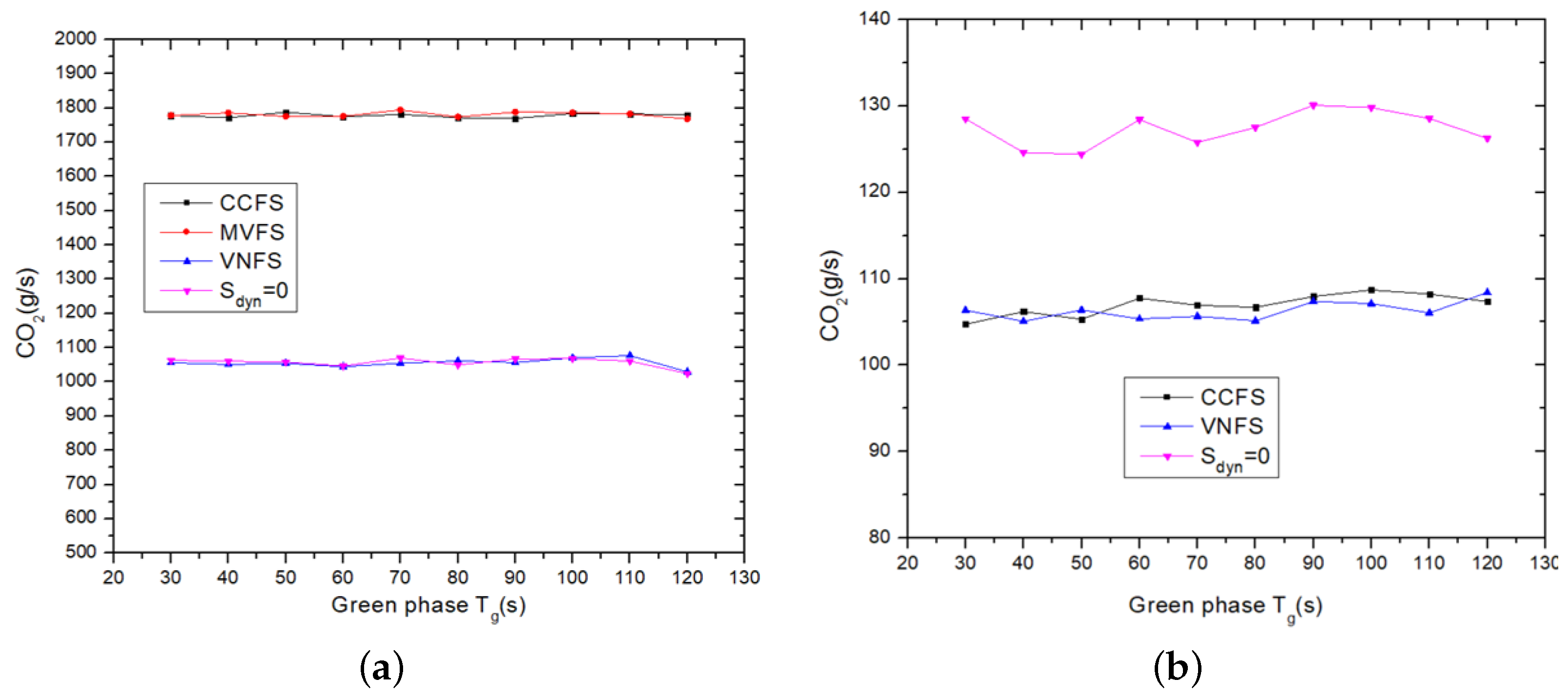
In addition, the impact of the green light period on CO₂ is depicted in Figure 5. This figure shows the CO₂ emissions as a function of $T_g$ at low ($\beta =0.2$) and high ($\beta =0.9$) extraction rates $\beta$ for the three strategies and for the case $S_{dyn}=0$. In both cases, i.e., $\beta =0.2$ and $\beta =0.9$, the duration of $T_g$ has no impact on CO₂ emissions, as they remain almost constant for all strategies. In the case of $\beta =0.2$ (Figure 5a), $S_{dyn}=0$ and VNFS exhibit lower emissions compared to CCFS and MVFS. Specifically, VNFS shows a reduction of approximately 40% in CO₂ emissions at low extraction rates compared to the other strategies. Nevertheless, for $\beta$ = 0.9, VNFS and CCFS display lower emissions compared to $S_{dyn}=0$ and MVFS (this difference is not depicted in Figure 5b due to the higher values where the difference between other strategies becomes less clear). At high extraction rates, VNFS achieves a reduction of about 16% in emissions relative to the others. Hence, the VNFS strategy demonstrates lower emissions at both low and high extraction rates.

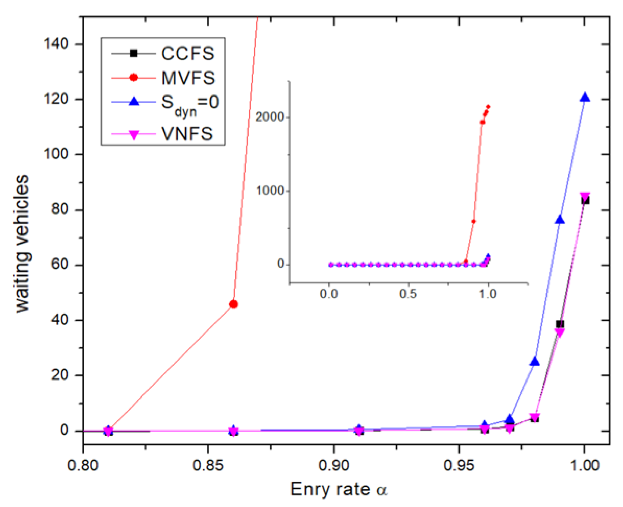
3.3. Influence of Waiting Vehicles on CO₂ Emissions

As mentioned earlier, all the previous works did not consider the waiting queue formed because vehicles cannot enter the system. Figure 6 depicts the waiting queue length using the three strategies and the random case $S_{dyn}=0$.

The waiting queue length is almost negligible at low and intermediate entry rates. Nonetheless, the increase in the waiting queue is noticeable when $\alpha >0.95$ for VNFS, CCFS, and a random case and when $\alpha >0.85$ for MVFS. Within these intervals, MVFS exhibits the highest queue length. Moreover, VNFS and CCFS display lower lengths compared to $S_{dyn}=0$ and MVFS. Thus, a significant number of vehicles are waiting to enter the system, contributing to CO₂ emissions, an important consideration in the analysis.

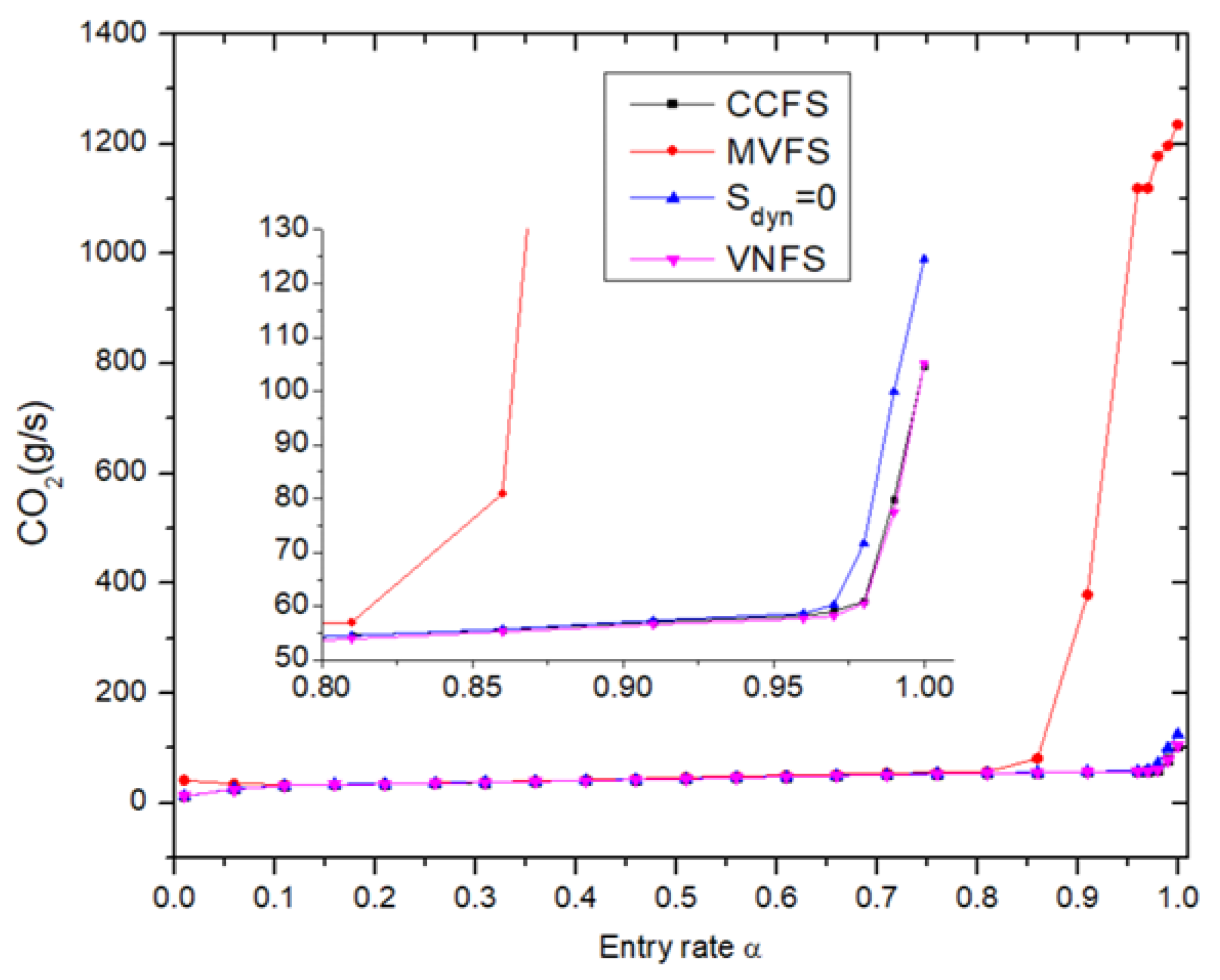
Considering the waiting queue at the entrance changes the behavior of CO₂ emissions, as shown in Figure 7. For $\alpha <0.95$, VNFS, CCFS and $S_{dyn}=0$ exhibit identical CO₂ emissions. When $\alpha <0.16$, MVFS presents higher CO₂ emissions; afterward, it shows the same emissions as VNFS, CCFS, and $S_{dyn}=0$. At high $\alpha$ values, CO₂ emissions augment significantly using MVFS, whereas VNFS and CCFS exhibit lower CO₂ emissions compared to the random case ($S_{dyn}=0$).

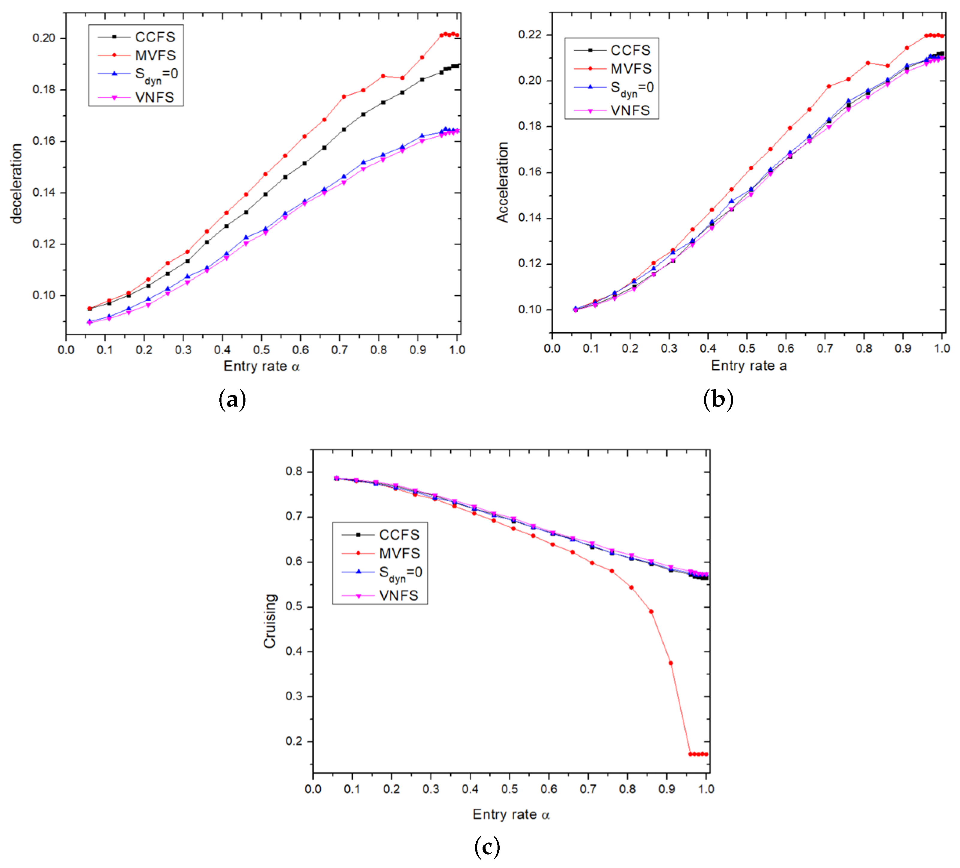
For a more detailed analysis, we plotted the cruising, acceleration, and deceleration rates using the three strategies and the random case (Figure 8). In all scenarios, acceleration and deceleration rates rise as the entry rate increases. As more vehicles enter the system, the headway between them diminishes, fostering increased interactions and, consequently, higher acceleration and deceleration processes, coupled with a decline in the cruising rate (constant speed).

On the other hand, VNFS demonstrates the lowest rates of acceleration/deceleration and the highest cruising rate compared to the other strategies. Meanwhile, MVFS exhibits the highest acceleration/deceleration processes and the lowest cruising rate. This explains why the system exhibited the lowest emissions when adopting VNFS.

3.4. Impact of Extraction Rate on CO₂ Emissions

Another limitation of previous studies is that they only utilized one value of $\beta$ ($\beta =1$), representing the deterministic case. In the following section, we will analyze the impact of the extraction rate on CO₂ emissions and flow.

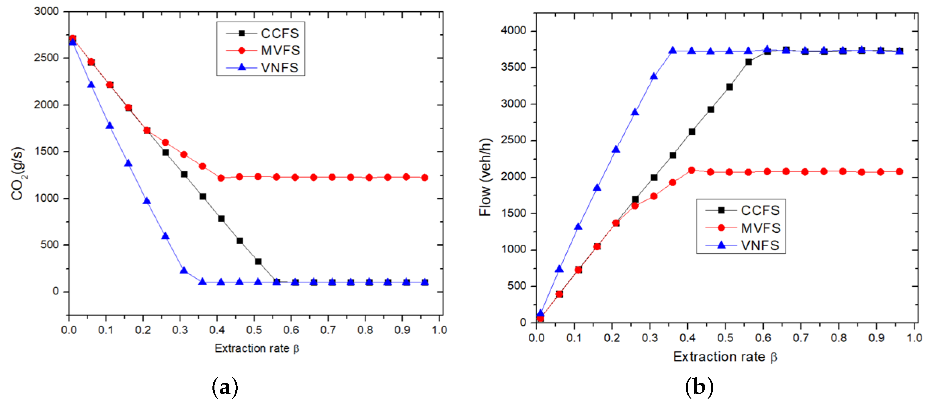
As shown in Figure 9, in both VNFS and CCFS, CO₂ emissions display two distinct phases; still, for MVFS, there are three phases. Initially, at low $\beta$ values, the traffic is in the congestion phase, which is characterized by slow vehicle movement and high acceleration and deceleration processes, leading to high CO₂ emissions (Figure 9a). As $\beta$ augments, emissions decline while the flow grows (Figure 9b) linearly. For MVFS, during its initial two phases, identified by their respective slopes, CO₂ emissions follow a similar pattern of decreasing until reaching a critical $\beta$ value (the same as the first phase for VNFS and CCFS). Beyond this critical threshold, CO₂ emissions and flow stabilize, even with a further increase in $\beta$, representing the second phase for VNFS and CCFS and the third phase for MVFS. This critical value marks the transition from the congestion phase to the free flow phase.

Moreover, for $\beta \le 0.2$, emissions using CCFS and MVFS are identical. However, CO₂ emissions become higher by opting for the MVFS. Furthermore, VNFS consistently exhibits the lowest CO₂ emissions compared to MVFS and CCFS. Yet, when $\beta >0.55$, VNFS and CCFS display identical emissions. Hence, VNFS demonstrates lower CO₂ emissions and better flow as a function of $\beta$.

3.5. Influence of Lane-Changing on CO₂ Emissions

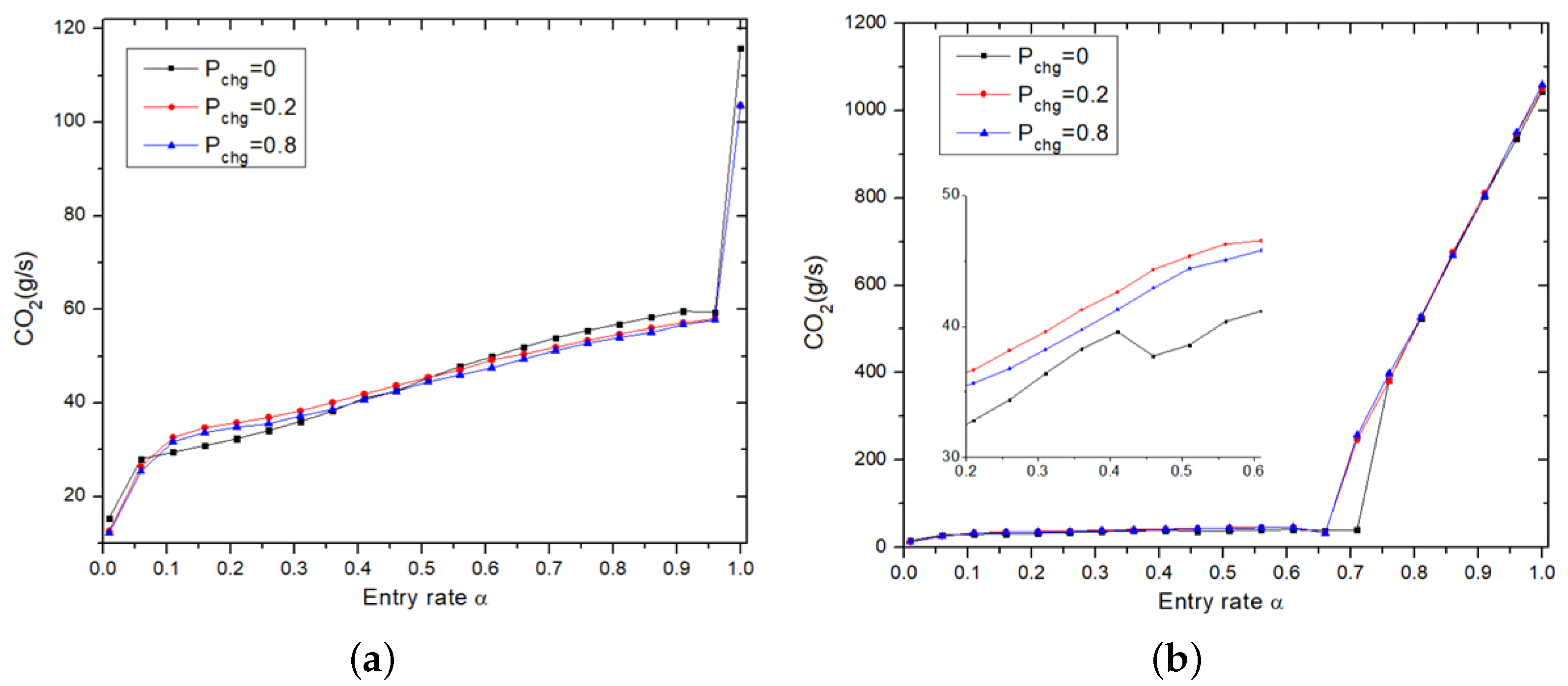
Figure 10 displays the impact of lane-changing probability by considering two different rates for beta ($\beta =0.2$ and $\beta =0.9$ ). For high $\beta$ values ($\beta =0.9$), the effect of $P_{chg}$ strongly depends on the entry rate $\alpha$. A critical $\alpha$ value exists, specifically $\alpha =0.5$, below which lane-changes increase CO₂ emissions. In this scenario, there is ample space between vehicles, rendering lane changes unnecessary and increasing CO₂ emissions without benefiting traffic flow. However, when $\alpha$ exceeds 0.5, lane changes improve traffic flow and decrease emissions. The high $\beta$ value allows most vehicles to exit the system without waiting, enabling fast vehicles to overtake slower ones and avoid congestion (Figure 10a).

At low $\beta$ values ($\beta =0.2$), within the $\alpha$ range of 0.11 and 0.7, the absence of lane changes correlates with a reduction in CO₂ emissions. In contrast, at very high $\alpha$ values, lane changes do not affect CO₂ emissions. This represents the jamming phase, characterized by a high influx of vehicles into the system and a low rate of exit (Figure 10b).

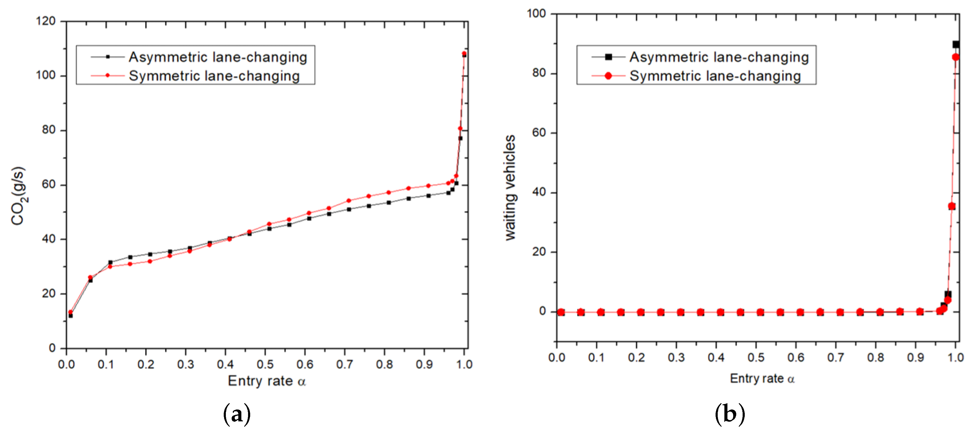
In addition, as explained above, lane-changing rules can be symmetric or asymmetric. Figure 11a illustrates CO₂ emissions using both lane-changing rules. At very low $\alpha$ values, CO₂ emissions are identical in both modes. Additionally, there is a critical $\alpha$ value ($\alpha \approx 0.41$) below which emissions are high when employing asymmetric lane-changing by approximately 6%; whereas, above it, emissions are elevated when adopting symmetric lane-changing. This behavior translates to a variation of about 6% in CO₂ emissions depending on the selected lane-changing mode.

To better understand this difference, and because both modes have almost the same number of waiting vehicles (Figure 11b), we calculated the congestion coefficient in both cases, i.e., symmetric and asymmetric lane-changing rules, using Equation (1). The results are shown in

Table 3. Values of congestion coefficient using symmetric and asymmetric rules.

	$\mathit{\alpha }=0.2$		$\mathit{\alpha }=0.8$
	Asymmetric Rules	Symmetric Rules	Asymmetric Rules	Symmetric Rules
Left lane	4	20	61	84
Right lane	29	11	85	78
Total	33	31	146	161

.

The congestion coefficient is slightly higher under asymmetric lane-changing rules for low $\alpha$ values ($\alpha =0.2$). Conversely, this coefficient increases using symmetric lane-changing rules at high $\alpha$ values ($\alpha =0.8$). Consequently, CO₂ emissions are lower during the free flow phase with symmetric rules; whereas in the congestion phase, emissions are minimized by adopting asymmetric rules.

3.6. Impact of Traffic Light Symmetry

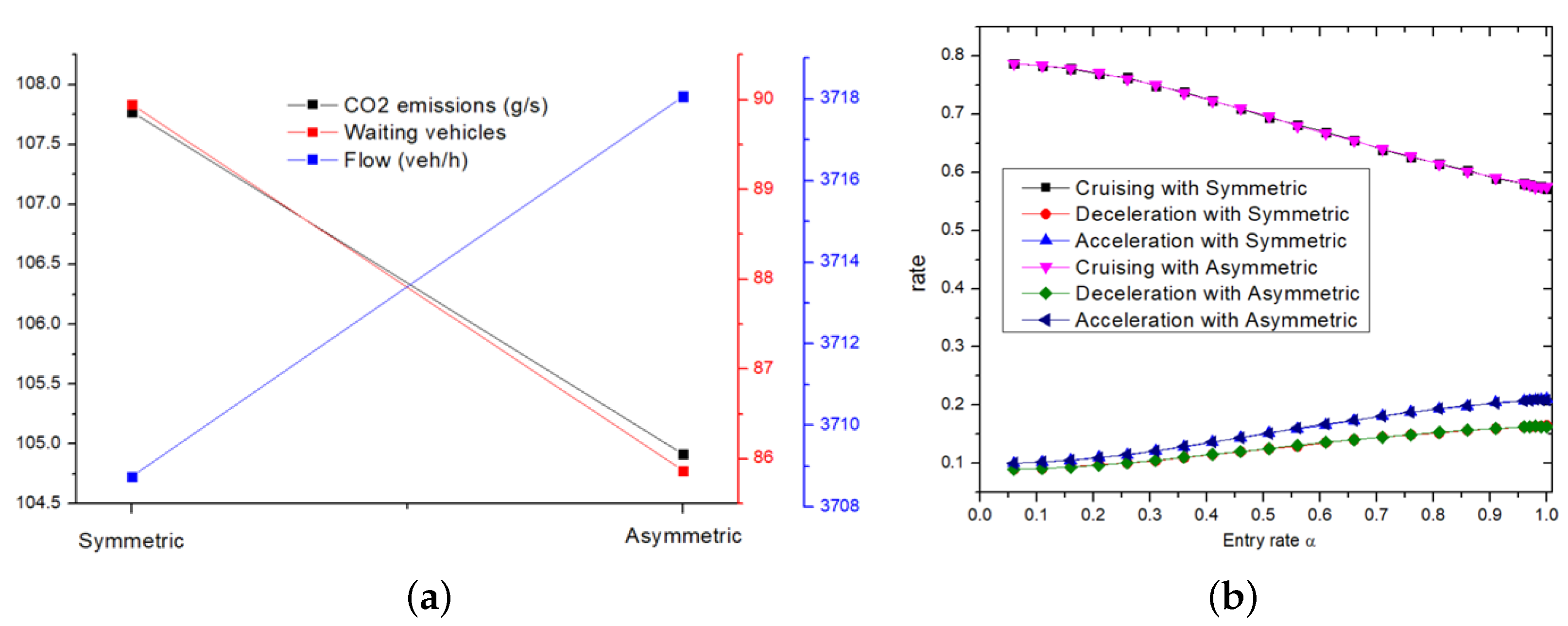
Another parameter impacting traffic emissions is the symmetry of traffic lights on both roads. As illustrated in Figure 12a, CO₂ emissions rise when symmetric traffic signals are utilized. Despite equal cruising, acceleration, and deceleration rates under both symmetric and asymmetric signalization schemes (Figure 12b), the divergence in CO₂ emissions stems principally from differences in the number of waiting vehicles. Notably, asymmetric traffic lights enable smoother ingress of vehicles, leading to decreased CO₂ emissions and enhanced flow. Notably, this result pertains to the case when $\alpha$ equals 1. Yet, when $\alpha$ is less than 1, emissions remain unchanged in both symmetric and asymmetric scenarios.

The findings of this study have clear implications for real-world traffic management and smart city deployment. The VNFS strategy, which relies on real-time vehicle count feedback near the system entrance, could be implemented using existing Intelligent Transportation Systems (ITS) infrastructure, such as connected vehicle networks, loop detectors, or smart cameras. By integrating VNFS into traffic control centers or vehicle-to-infrastructure (V2I) systems, urban planners can provide adaptive route recommendations that reduce vehicle queuing and CO emissions. In addition, given that feedback from the entire system does not provide any significant advantage over entrance-focused data, cities can minimize data collection complexity and cost while still achieving efficient traffic flow and environmental benefits. This makes the VNFS approach particularly suitable for gradual integration into existing smart mobility frameworks.

4. Discussion

Several limitations can be identified in previous works in the context of feedback strategy in two-route systems. These include a lack of consideration for waiting vehicles at the system entrance, as well as a focus on single-lane roads without accounting for lane-changing maneuvers. Additionally, previous studies have been limited to using deterministic cases for entry and extraction rates ($\alpha$ = 1 and $\beta$ = 1), without exploring the impact of variations in these parameters. Furthermore, the impact of traffic lights has not been thoroughly examined. Another notable limitation is the lack of modeling traffic emission in a two-route scenario using information feedback strategy, with only one work identified on this topic [51]. One of the most influential factors in emission dynamics is the number of vehicles waiting at the system entrance. Regarding vehicle entry methods in our two-route system, feedback strategies serve as representations, exerting influence not only on vehicles within the system but also on those waiting at the entrance, directly impacting traffic emissions. One crucial parameter affecting emissions is the number of waiting vehicles, which can be minimized through appropriate strategies, leading to reduced emissions. In this context, the impact of four strategies (VNFS, CCFS, MVFS, and random case) on CO₂ emissions and flow was analyzed and compared.

The extent of information feedback and communication influences the decision-making of incoming vehicles and consequently affects traffic emissions. The use of data from all vehicles within the system does not significantly improve traffic characteristics. The farther away the information (vehicle data) is from the entrance, the less impact it has on traffic capability (see Figure 2). Small DIS values can results in a reduction of approximately 8% in CO₂ emissions compared to larger feedback ranges. Therefore, it is sufficient to only consider the information feedback from the system entrance.

The effectiveness of various feedback strategies also significantly shapes emission and flow behavior, particularly at different traffic densities. In addition, the impact of feedback strategies is particularly significant at high densities ($\alpha >0.85$), where emissions can decrease and flow can increase compared to the random case. The best strategies for low values of $\beta$, representing the jamming phase, are VNFS and $S_{dyn}=0$ (see Figure 9). $S_{dyn}=0$ refers to a random route choice model, where vehicles select routes without feedback-based optimization. However, at high $\beta$ values, the most effective strategies are VNFS and CCFS. In [51], the best strategies were MVFS and CCFS; yet, in our case, MVFS is the least effective strategy due to higher CO₂ emissions, while CCFS can be effective only at higher values of $\beta$. Considering the aforementioned limitations, our results reveal different findings. This difference in results is attributed to the use of single-lane roads, homogeneous traffic, and neglecting the influence of density in previous works.

Using the VNFS strategy provides stability to the traffic system, thereby increasing vehicle influx to a peak of 3735 veh/h, reducing vehicle queuing and consequently reducing traffic-related emissions, reaching a minimum of approximately 100 g/s in comparison to the 1200 g/s of MVFS. Moreover, the effect of the extraction rate $\beta$ ceases at the transition point from the congestion phase to the free flow phase; as shown in Figure 9, further increases in $\beta$ during free flow do not have any effect on CO₂ emissions. This suggests that in such a scenario, priority can be given to other roads connected to the studied system, where the probability of vehicle exit does not necessarily need to be very high. For instance, in the case of VNFS, a $\beta$ value of 0.4 or greater is sufficient to significantly improve the efficiency of the traffic network.

Beyond the impact of feedback strategies, lane-changing dynamics play a critical role in shaping emissions patterns, particularly under varying traffic densities. Additionally, the impact of lane-changing on CO₂ emissions was examined through an analysis of the influence of $P_{chg}$ and lane-changing modes.

When $\beta$ is high, and $\alpha$ is low, changing lanes does not improve CO₂ emissions and increases them. In such cases, changing lanes is unnecessary due to the wide gaps between vehicles. Nevertheless, the dynamics shift when $\alpha$ is high. In this scenario, changing lanes enables faster vehicles to overtake slower ones, thereby reducing CO₂ emissions (see Figure 10a). Conversely, at lower $\beta$ values, abstaining from lane changes decreases CO₂ emissions at intermediate $\alpha$ values, with approximately 6%; while CO₂ emissions remain consistent for other $\alpha$ values across all $P_{chg}$ values (see Figure 10b).

Lane-changing impacts are deeply intertwined with traffic density levels, leading to contrasting outcomes depending on $\alpha$ and $\beta$ values. Furthermore, the mode of lane-changing impacts CO₂ emissions differently depending on the traffic density level. For $\alpha$ values below approximately 0.4, asymmetric lane-changing generates higher emissions, whereas symmetric lane-changing yields elevated emissions when $\alpha$ surpasses this threshold as shown in Figure 11a. This difference in CO₂ emissions is not attributed to variations in the number of waiting vehicles as both scenarios exhibit comparable numbers of waiting vehicles. Instead, it is due to the degree of congestion generated by each type of lane-changing. Asymmetric rules generate a low congestion coefficient (141 in comparison with 161 of symmetric rules), when $\alpha <0.41$; however, this coefficient is low when using symmetric rules (31 in comparison with 33 of asymmetric rules) when $\alpha \le 0.41$ (see Figure 12 and Table 3).

The effect of lane-changing rules on traffic emissions varies based on the road’s geometry and features. Simulation results at intersections indicate that the system displays lower traffic emissions when utilizing symmetric lane-changing rules instead of asymmetric rules [11]. In our specific two-route scenario, each lane-changing mode can decrease CO₂ emissions within a specific range of entry rates.

At times, it may not be recommended to rely solely on a single mode of control to optimize traffic characteristics for all traffic states. Traffic control strategies should be adaptable based on traffic-related parameters.

Scholars have also shown interest in exploring traffic dynamics with autonomous vehicles, considering them a promising solution to traffic-related challenges, including emissions [72,73].

The result presented in this study holds applicability in autonomous and connected vehicle systems, enabling vehicles to communicate and make lane-changing decisions based on traffic conditions to minimize CO₂ emissions in a two-route system.

Moreover, when $\alpha =1$, CO₂ emissions increase by deploying symmetric traffic lights. While cruising, acceleration, and deceleration rates remain consistent between symmetric and asymmetric traffic light systems, variations in CO₂ emissions primarily arise from differences in waiting vehicle numbers. Asymmetric traffic lights promote smoother vehicle entrance, reducing CO₂ emissions and improving flow efficiency. Otherwise, emissions remain constant regardless of whether traffic signals are symmetric or asymmetric when $\alpha$ < 1.

A slight adjustment in traffic parameters, such as a further increase in $\alpha$ or $\beta$ (e.g., from $\alpha =0.99$ to $\alpha =1$), can significantly modify the system’s behavior across different scenarios, including symmetric/asymmetric lights, different feedback strategies, and lane-changing rules. This illustrates the complexity of traffic dynamics, wherein even minor parameter changes can have substantial effects. This highlights how traffic flow characteristics can vary in response to different traffic parameters.

When homogeneous systems are examined regarding their symmetries, heterogeneity represents a form of symmetry breaking. At times, the system’s symmetry is disrupted to maintain state symmetry [74]. This concept can be utilized to control and enhance complex systems’ stability by incorporating heterogeneity [65,75]. This finding is applicable to the current system under study, where breaking the symmetry of lane-changing rules can improve system stability and reduce CO₂ emissions when $\alpha$ is greater than 0.4. Likewise, breaking the symmetry of traffic lights can help minimize emissions when $\alpha$ equals 1. Future studies should explore the real-world feasibility of implementing VNFS and asymmetric traffic light systems, considering aspects such as driver compliance, infrastructure costs, and the availability of real-time traffic data.

In terms of real-world applicability, the implementation of strategies such as asymmetric traffic lights and the VNFS approach would require careful consideration of infrastructure feasibility, driver compliance, and data communication systems. Deploying asymmetric lights may involve changes to signal programming and coordination, while VNFS depends on reliable vehicle-to-infrastructure (V2I) communication to inform route decisions in real time. Furthermore, driver behavior and acceptance of such automated guidance must be evaluated to ensure effectiveness. These factors highlight the importance of bridging simulation-based findings with practical deployment strategies in smart city environments.

5. Conclusions

This study investigates traffic emissions and flow dynamics optimization in a two-route scenario using various information feedback strategies: VNFS, CCFS, MVFS, and $S_{dyn}=0$ (random route selection). This research provides valuable insights by addressing previous limitations such as single-lane analysis, traffic homogeneity, and deterministic entry/extraction rates. Simulation results show that utilizing data from all vehicles within the system does not significantly improve traffic characteristics. Instead, focusing on information feedback from the system’s entrance is sufficient.

Moreover, traffic lights contribute to increased CO₂ emissions due to acceleration and deceleration processes at traffic lights, with a critical inflection point observed at $\alpha =0.11$ and $\alpha =0.16$, respectively, with and without traffic lights. Moreover, CO₂ emissions in all strategies can be expressed as a polynomial of the ninth degree in terms of $\alpha$.

Compared to other strategies, and in contrast to the previous works, VNFS exhibits reduced acceleration/deceleration processes and higher cruising rates, enhancing system stability and lowering CO₂ emissions. These findings are especially relevant for urban transportation infrastructure design and optimization.

Furthermore, a critical threshold exists for $\beta$ ($\beta \approx 0.55$), beyond which CO₂ emissions and flow stabilize. VNFS consistently outperforms MVFS and CCFS. Notably, VNFS demonstrates lower emissions and improved flow as $\beta$ increases.

The study explored the impact of lane-changing on CO₂ emissions depending on lane-changing modes and $P_{chg}$ values. Results suggest that under high $\beta$ and low $\alpha$ conditions, lane changes increase the CO₂ emissions due to wide vehicle gaps. Conversely, at higher $\alpha$ values, lane changes enable faster vehicles to overtake slower ones, consequently decreasing CO₂ emissions.

At lower $\beta$ values, avoiding lane changes decreases emissions at specific $\alpha$ values, while emissions remain consistent across other $\alpha$ values for all $P_{chg}$ values. Additionally, there is a critical $\alpha$ value ($\alpha \approx 0.41$) below which emissions are high when employing asymmetric lane-changing; while above it, emissions are elevated when adopting symmetric lane-changing. Finally, asymmetric traffic lights reduce CO₂ emissions when $\alpha =1$, whereas no significant changes are observed for $\alpha <1$.

These conclusions support future efforts to integrate dynamic feedback and lane-changing strategies in intelligent infrastructure systems aimed at reducing urban emissions.