Empirical Investigation of the Effects of the Measurement-Data Size on the Bayesian Structural Model Updating of a High-Speed Railway Bridge

Abstract

Bayesian structural model updating (SMU) is among the most powerful methods for estimating the bending stiffness and modal damping of high-speed railway (HSR) bridges and predicting their bridge-response-based resonance responses. Although studies indicated that the convergence to the true value as the observed data increase favored Bayesian inference, the data-size effects on the estimation accuracy have not been sufficiently investigated. Here, the maximum bridge deck acceleration upon the passage of a train, which is used in European bridge designs, is explored, and the data-size effect on the Bayesian SMU is empirically investigated. For an HSR bridge spanning approximately 50 m, the parameters and maximum acceleration of a beam model on which the moving loads act are updated by the Markov chain Monte Carlo simulation method using the measured maximum acceleration. A comparison of the estimated values with different measurement data revealed that the estimated values converged for three samples, when the data included the resonance state of the test bridge. Overall, the results can be employed to establish a logical method for determining the necessary field measurement specifications for ensuring the accuracy of Bayesian SMU.

1. Introduction

It is well established that the resonance caused by trains traveling at high speeds constitutes a major factor that increases the resonance responses of high-speed railway (HSR) bridges [1,2]. Based on the results of extensive studies, many countries globally have stipulated bridge-response limits during resonance in design standards [3,4,5]. Resonance occurs in HSRs when the excitation frequency, which is determined by the regular axle arrangement of the running train, approaches the bridge (first bending mode) frequency $\mathit{f}$ [1,2]. The magnitudes of the increased displacements and accelerations during resonance mainly depend on the bridge length and modal damping ratio ($\mathit{\xi }$; and additional damping from the vehicle) [3,5]. Recent HSR bridge designs generally comprise measures to safely set the bridge frequencies and modal damping ratios, thus largely eliminating the issue of excessive vibration due to resonance at the initial speed of trains [6]. Similarly, the frequencies of some non-recent HSR bridges in some countries have been reduced by aging and the progression of cracks in the concrete; resonance occurrences due to proximity to the excitation frequency of a running train have been reported [7,8]. Notably, the increases in the speeds of recent high-speed trains have induced resonance when the excitation frequencies of running trains approach $\mathit{f}$ [9].

Thus, investigating bridge frequencies (flexural stiffnesses) and $\mathit{\xi }$, which are related to the resonance, to properly manage the resonance and excessive vibration of such HSR bridges is crucial to the proper management of the resonance and excessive vibrations of such HSR bridges [10,11]. Additionally, the additional damping ratios and additional masses due to the dynamic interaction between the traveling vehicle and bridge during the passing of trains affect HSR bridges [12]. Thus, methodologies, such as identification methods for bridge frequencies and $\mathit{\xi }$s, as well as the Bayesian updating of bridge numerical models based on bridge responses during actual operation (during the train’s passing) [12,13], have been consistently proposed [14,15]. Notably, Bayesian structural model updating (SMU) represents an efficient methodology for updating the material parameters of a structural calculation model based on the general finite-element method to match the observed data [16]. Following Beck et al.’s [17] pioneering study, the Bayesian SMU methodology has developed rapidly in recent years [18]. Several Bayesian SMU methods similar to those reported in this paper have been reported for railway bridges during the traveling of trains [14,15]. In particular, Bayesian SMU has been recognized as a promising approach for addressing existing challenges in model updating by explicitly accounting for uncertainty. For instance, Ierimonti et al. [19], who applied a Bayesian learning model to the structural health monitoring (SHM) of historical structures, highlighted that one of the key advantages of Bayesian model updating lies in its ability to handle inherent ill-posedness and non-uniqueness in the model updating process. This advantage is significant not only within the context of SHM but also from the broader perspective of evaluating the resilience of systems against disasters [20]. Furthermore, in addition to conventional batch Bayesian SMU using collected datasets, sequential updating techniques—such as data assimilation and Bayesian filtering, which update the model each time new data are acquired—have also been proposed in recent years [21]. Bayesian SMU employs Bayes’ theorem to update the parameters of the structural model to ensure they match the observed values. Numerous studies emphasized two advantages of employing Bayes’ theorem. First, it facilitates the evaluation of the optimal values of the parameters and their uncertainties based on posterior distributions ($\mathrm{P}\left(\mathit{\theta }|\mathit{D}\right)$) [16,17]. Second, gradually increasing small amounts of observation data will cause the convergence of the $\mathrm{P}\left(\mathit{\theta }|\mathit{D}\right)$ to the population distribution, thereby improving the estimation accuracy [18,22]. The effectiveness of the first advantage has been demonstrated via uncertainty assessment and reliability designs [15,18]. However, although numerous scholars demonstrated the advantages of the influence of the number of observation data, only a few have demonstrated the effectiveness of these data sizes on the Bayesian SMU of HSR bridges. Moreover, the number of observation data required to obtain a highly accurate $\mathrm{P}\left(\mathit{\theta }|\mathit{D}\right)$ for existing HSR bridges using Bayesian SMU directly affects the required field-measurement period, and this is effort- and cost-intensive. Therefore, determining the number of observation data required for Bayesian SMU is important information that is directly linked to the effort and cost required for the state and response evaluations of existing HSR bridges.

Based on the foregoing, this study was aimed at investigating the effect of the on-site-measured acceleration data sizes on the $\mathrm{P}\left(\mathit{\theta }|\mathit{D}\right)$ obtained by Bayesian SMU of an actual HSR bridge. Additionally, the effects of sensor fusion and data quality on the estimation accuracy were discussed based on the estimation of $\mathrm{P}\left(\mathit{\theta }|\mathit{D}\right)$ of cases using accelerometers at multiple locations, as well as including observation data from the resonance region. Finally, the crucial findings were clarified regarding the sampled acceleration-data size required for the Bayesian SMU of the test HSR bridge. This study was not aimed at clarifying the HSR bridge phenomenon; rather, it was conducted to clarify the statistical properties that depend on the observation-data size. Thus, a theoretical solution of the elastic support beam, which is relatively simple as well as exhibiting few parameters, was utilized as a numerical model of the bridge [23]. Additionally, a moving-load model was deployed as the traveling train. Notably, the obtained parameters for $\mathit{f}$, $\mathit{\xi }$, and bearing capacity included dynamic interactions with the train system owing to these constraints on the numerical model. Further, the Markov chain Monte Carlo simulation (MCMC) method, a numerical solution method for Bayesian updating, was adopted as the methodology for updating the numerical model [8,12]. The remainder of this paper is structured as follows: Section 2 describes the test bridge, measurement method, numerical model, and Bayesian SMU method, and Section 3 presents the Bayesian updating results and discusses those results. Finally, Section 4 concludes the study.

2. Measurement and Model Updating Methods

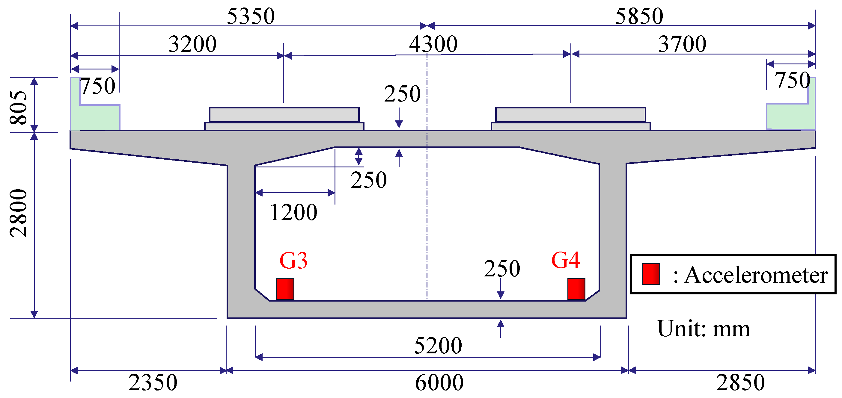
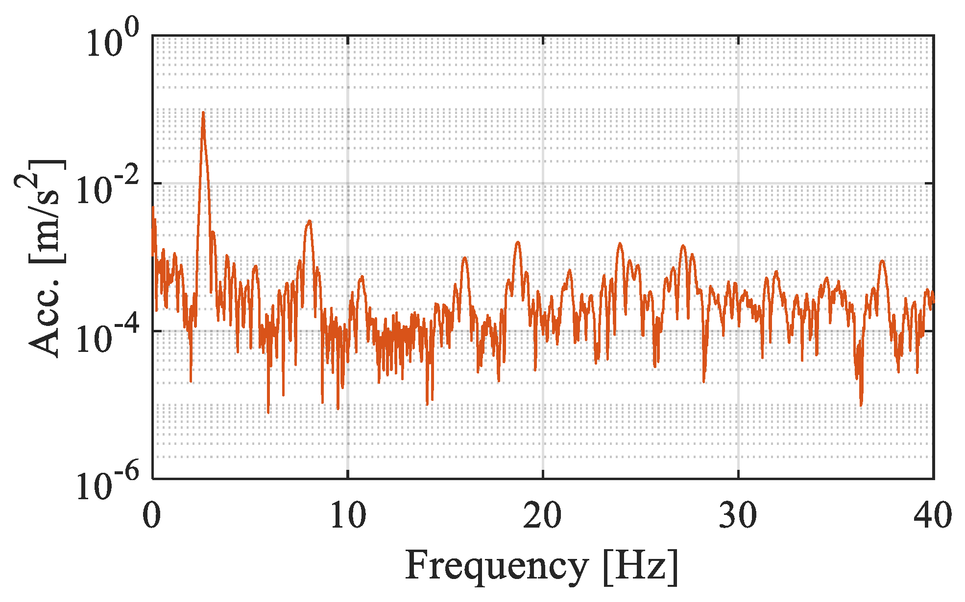
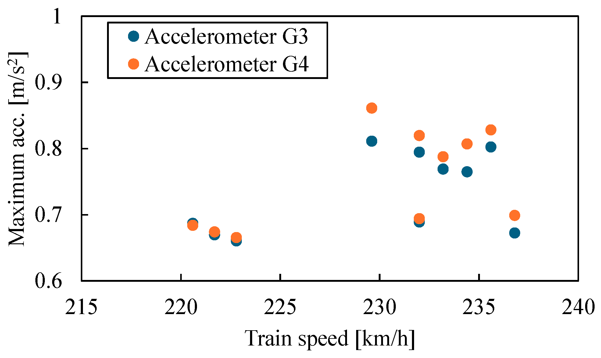
2.1. Test Bridge and Measurement Method

Figure 1 shows a cross-section of the test bridge. The test bridge is a 1-box PC box girder double-track bridge (length: 48.6 m), representing a standard operational HSR bridge. In this study, the slab track was adopted. This bridge comprises a rubber-type bearing to ensure the earthquake resistance of the piers; thus, the support stiffness $k_v$ was lower than that of the general bearings.

As shown in Figure 1, the acceleration responses when the train passed the bridge were measured using two accelerometers (G3 and G4) installed on both sides of the bridge midspan. Further,

Table 1. Specifications of the measurement equipment.

Devices	Specifications
Piezoelectric Accelerometers (PV-85; Rion Co., Ltd., Kokubunji, Japan)	Frequency range: 1–7000 Hz Sensitivity: 6.42 pC/(m/s2)
Preamplifier (NH-22; Rion Co., Ltd.)	Frequency range: 1–10,000 Hz
A/D Converter (Ni cDAQ-9172·Ni9233; National Instruments Japan Co., Ltd., Tokyo, Japan)	Sampling frequency: 2000–10,000 Hz
Control System (Labview)	Multipoint synchronization Sampling frequency: 2000 Hz
Laptop PC (CF-SV; Panasonic Co., Ltd., Kadoma, Japan)	CPU: i5 4.4 GHz Memory capacity: 16 GB

presents the specifications of the measurement equipment. The acceleration data were recorded on a laptop computer at 2 kHz. The acceleration responses as the train passed were processed using a 30 Hz low-pass filter (LPF), following the deck acceleration limit for European HSR bridges [5,9], and deployed for the Bayesian SMU described below. The speed of the trains crossing the test bridge was set to 220–236 km/h. Furthermore, the acceleration data of the crossing of 10 trains (8-car trains) were used.

Additionally, the test bridge was subjected to bridge modal identification by multipoint acceleration measurement; thus, the first bending mode was determined as approximately 2.6 Hz [24]. Figure 2 shows the measured acceleration spectrum obtained by G3 during the passing of a train (train speed: 235 km/h). The vibration component corresponding to $\mathit{f}$ of the first bending mode dominated when a train passed, and no other dominant components were observed up to 30 Hz. Therefore, the theoretical solution of an elastically supported beam [23] was adopted as the numerical model, as will be described in this paper.

Figure 3 shows the relationship between the maximum values of the 30 Hz-LPF acceleration response measured by G3 and G4, as well as the train speed (vehicle length: 25 m). Therefore, the resonant speed was 2.5 × 25 = 62.5 [m/s] = 234 [km/h] [24]. The acceleration was relatively large when the train traveled at 230 km/h. Notably, the peak train speed of the maximum acceleration in the measurement results was slightly lower than the theoretically calculated value. This might be due to the added mass effect, which accounts for a dynamic interaction with the vehicle. As elucidating the vibration phenomenon observed when trains cross HSR bridges is beyond the scope of this study, readers are referred to Reference [12] for the added mass effect.

Here, the maximum acceleration (Figure 3) was used as the observed data to investigate the effects of the number of samples on the Bayesian SMU. Specifically, the $\mathrm{P}\left(\mathit{\theta }|\mathit{D}\right)$s of the structural parameters using the Bayesian SMU described below were estimated for the following cases:

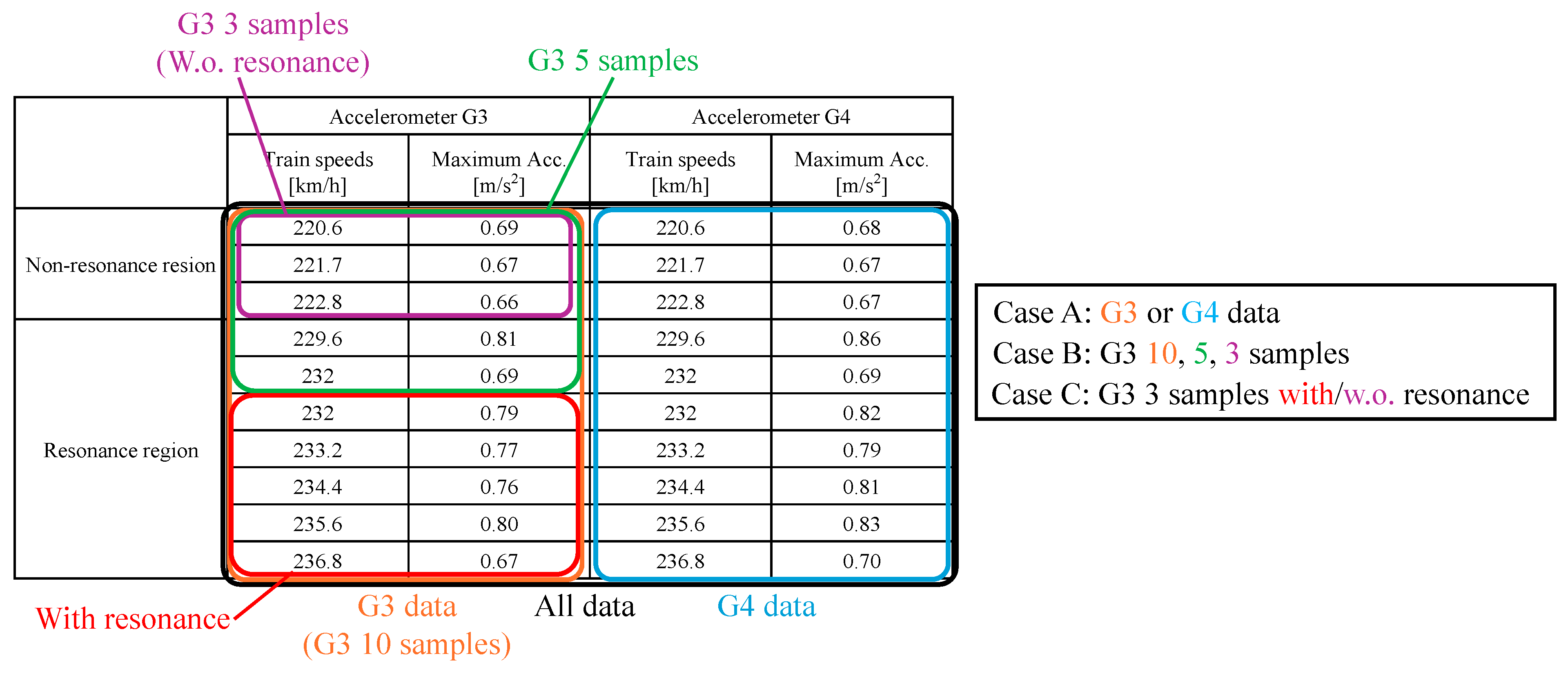
• All data (the all observation data from G3 and G4);
• Case A: G3 or G4 data;
• Case B: 10, 5, 3 samples from G3 data;
• Case C: with/without (w.o) resonance from G3 data.

The relationship between the data used in each case and the entire dataset is illustrated in Figure 4.

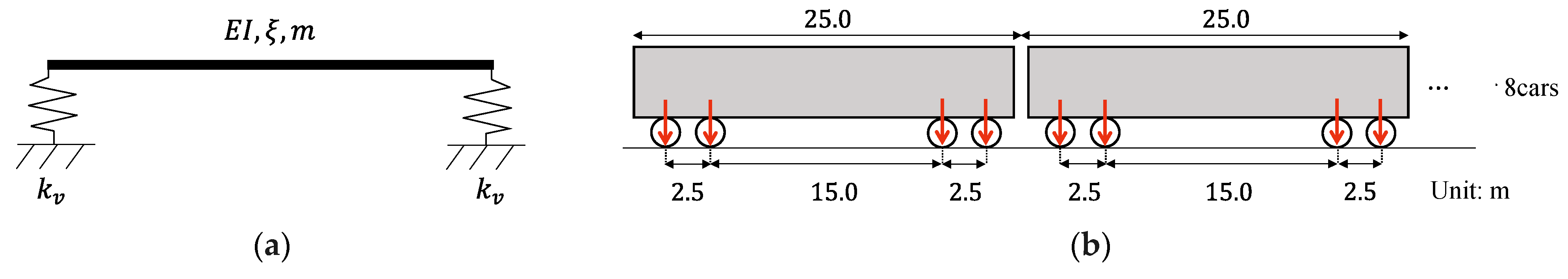
2.2. Structural Modeling

Figure 5 shows the elastic supported-beam model employed in this study. The rubber bearings were modeled as springs (bearing-spring constant $k_v$) based on their responses. The bridge exhibited a uniform cross-section; it was a Euler beam exhibiting the following parameters: bending stiffness $EI$, $\mathit{\xi }$, and unit-length mass $\mathit{m}$. The traveling train was modeled as a moving load exhibiting the same axle arrangement as the train. As aforementioned, this study was aimed at exploring a bridge in which the primary bending mode accounted for the main component during the passing of trains. Thus, this simple structural model adequately reproduced the response when the trains passed the bridge. However, this is limited to cases where there is no damage in the track or structure, and the mass of the bridge is sufficiently large compared to that of the vehicle. Specifically, this condition applies to medium to long-span concrete bridges with slab track systems, which are the focus of this study. The accurate reproduction of the response by this model was confirmed by comparing it with the measured response reported at the end of this section.

Similar to References [23,25], the bridge response during the passing of a train was calculated by superimposing the closed-form solution of the beam response under the action of a single moving load $\mathit{P}$ derived from the model in Figure 4, with a phase shift. Notably, the closed-form solution is derived, as follows:

Consider a situation where the left end of the beam was 0, while the horizontal distance $\mathit{x}$ was defined, and where a downward load $P$ moves on the beam from the left to right end at a constant speed $\mathit{v}$. Here, the displacement $\mathit{w}$ of the beam at position $\mathit{x}$ is expressed using the following equation based on the motion method of the beam:

$$\mathit{m}{\displaystyle \frac{{\partial }^{2}w}{\partial t^2}}+\mathit{E}\mathit{I}{\displaystyle \frac{{\partial }^{4}w}{\partial x^4}}=\mathit{P}\mathit{\delta }\left(x-vt\right),$$

(1)

$$\mathit{\delta }\left(u\right)=\left\{\begin{array}{c}1, u=0\\ 0, u\ne 0\end{array}\right..$$

(2)

The beam displacement was modally decomposed using Equations (3) and (4), as follows:

$$\mathit{w}\left(x,t\right)\approx {\varphi }^0\left(x\right)\mathit{q}\left(t\right),$$

(3)

where ${\varphi }^0\left(x\right)$ denotes the unnormalized first-order bending-mode shape. Thus, by setting $\mathit{q}\left(t\right)=\mathit{exp}\left(i\omega t\right)$, the equation of the motion of the free-vibration system without damping (Equation (1)) can be expressed, as follows:

$${\displaystyle \frac{{\partial }^4{\varphi }^0\left(x\right)}{\partial x^4}}-{\omega }^2{\displaystyle \frac{m}{EI}}{\varphi }^0\left(x\right)=0,$$

(4)

where $\mathit{\omega }$ is the natural circular frequency, and $\mathit{\omega }=2\mathit{\pi }\mathit{f}$ ($\mathit{f}$ is the bridge frequency).

To derive Equation (4), $\mathit{\beta }$ is denoted as it satisfies the following relation:

$${\beta }^4={\omega }^2{\displaystyle \frac{m}{EI}}.$$

(5)

Further, the general solution of ${\varphi }^0$ is expressed by the following equation:

$${\varphi }^0\left(x\right)=A^0\cos \left(\beta x\right)+B^0\sin \left(\beta x\right)+C^0\mathit{cosh}\left(\beta x\right)+D^0\mathit{sinh}\left(\beta x\right).$$

(6)

By considering $\xi =c/2m\omega$, the equation of motion in modal coordinates can be expressed, as follows:

$$\ddot{q}\left(t\right)+2\mathit{\omega }\mathit{\xi }\dot{q}\left(t\right)+{\omega }^2\mathit{q}\left(t\right)=\mathit{P}\mathit{\varphi }\left(vt\right),$$

(7)

$$\mathit{\varphi }\left(x\right)={\displaystyle \frac{{\varphi }^0\left(x\right)}{m{\int }_{x=0}^L{\varphi }^0{\left(x\right)}^{2}dx}},$$

(8)

where $\mathit{\varphi }\left(x\right)$ is in the mass-normalized mode form, which is calculated by the integral calculations of the denominator in Equation (8).

Equation (9) for the unknown variable β can be obtained based on the boundary conditions of the rotation and displacement at the beam ends.

$$\left|{\mathit{\Gamma }}_{\mathit{\beta }}\right|=0,$$

(9)

$${\mathit{\Gamma }}_{\mathit{\beta }}=\left[\begin{array}{c}{\mathit{\Gamma }}_{\mathbf{1}}\\ {\mathit{\Gamma }}_{\mathbf{2}}\end{array}\right],$$

(10)

$${\mathit{\Gamma }}_{\mathbf{1}}=\left[\begin{array}{cccc}-EI{\beta }^2& 0& EI{\beta }^2& 0\\ k_v& EI{\beta }^3& k_v& EI{\beta }^3\end{array}\right],$$

(11)

$${\mathit{\Gamma }}_{\mathbf{2}}={\left[\begin{array}{cc}-EI{\beta }^2\mathit{cos}\left(\beta L\right)& EI{\beta }^3\mathit{sin}\left(\beta L\right)+k_v\mathit{cos}\left(\beta L\right)\\ -EI{\beta }^2\mathit{sin}\left(\beta L\right)& -EI{\beta }^3\mathit{cos}\left(\beta L\right)+k_v\mathit{sin}\left(\beta L\right)\\ EI{\beta }^2\mathit{cosh}\left(\beta L\right)& EI{\beta }^3\mathit{sinh}\left(\beta L\right)+k_v\mathit{cosh}\left(\beta L\right)\\ EI{\beta }^2\mathit{sinh}\left(\beta L\right)& EI{\beta }^3\mathit{cosh}\left(\beta L\right)+k_v\mathit{sinh}\left(\beta L\right)\end{array}\right]}^T.$$

(12)

By solving Equation (9), Equation (5) can also be derived as a differential equation with respect to $\mathit{t}$, as $\mathit{\beta }$ becomes known. In this study, a closed-form solution derived using the Laplace transform [25], which is a reformulation of Reference [23], was employed.

The Laplace transform was performed for Equation (7), and $\mathit{q}\left(t\right), \dot{q}\left(t\right), \ddot{q}\left(t\right)$ were calculated by the inverse Laplace transform with the initial conditions $\mathit{q}\left(0\right)=0, \dot{q}\left(0\right)=0$. Particularly, the calculation results for $\ddot{q}\left(t\right)$ are presented below.

$$\ddot{q}\left(t\right)={\displaystyle \frac{AP}{V_1^2+V_3^2}}{\ddot{E}}_1+{\displaystyle \frac{BP\beta v}{V_1^2+V_3^2}}{\ddot{E}}_2+{\displaystyle \frac{CP}{V_2^2-V_3^2}}{\ddot{E}}_3+{\displaystyle \frac{DP\beta v}{V_2^2-V_3^2}}{\ddot{E}}_4,$$

(13)

$${\ddot{E}}_1={\omega }^2{H}_0\left[{\displaystyle \frac{\omega }{{\omega }_d}}\left\{{\omega }^2-{\left(\beta v\right)}^2\left(3-4{\xi }^2\right)\right\}+\left\{{\omega }^2-{\left(\beta v\right)}^2\left(1-4{\xi }^2\right)\right\}\right]-{\left(\beta v\right)}^2{H}_1,$$

(14a)

$${\ddot{E}}_2=\mathit{\omega }{H}_0\left[{\displaystyle \frac{\omega }{{\omega }_d}}\left\{{\omega }^2-{\left(\beta v\right)}^2\left(1-2{\xi }^2\right)\mathit{sin}\left({\omega }_{d}t\right)\right\}-2\xi {\left(\beta v\right)}^2\mathit{cos}\left({\omega }_{d}t\right)\right]+\mathit{\beta }\mathit{v}{H}_2,$$

(14b)

$${\ddot{E}}_3={\omega }^2{H}_0\left[{\displaystyle \frac{\omega }{{\omega }_d}}\left\{{\omega }^2+{\left(\beta v\right)}^2\left(3-4{\xi }^2\right)\right\}+\left\{{\omega }^2+{\left(\beta v\right)}^2\left(1-4{\xi }^2\right)\right\}\right]-{\left(\beta v\right)}^2{H}_3,$$

(14c)

$${\ddot{E}}_4=\mathit{\omega }{H}_0\left[{\displaystyle \frac{\omega }{{\omega }_d}}\left\{{\omega }^2+{\left(\beta v\right)}^2\left(1-2{\xi }^2\right)\mathit{sin}\left({\omega }_{d}t\right)\right\}+2\xi {\left(\beta v\right)}^2\mathit{cos}\left({\omega }_{d}t\right)\right]+\mathit{\beta }\mathit{v}{H}_4,$$

(14d)

$${\omega }_d=\mathit{\omega }\sqrt{1-\xi },$$

(14e)

$$V_1={\left(\beta v\right)}^2-{\omega }^2, V_2={\left(\beta v\right)}^2+{\omega }^2, V_3=2\mathit{\omega }\mathit{\xi }\mathit{\beta }\mathit{v}, V_4=2\mathit{\omega }\mathit{\xi },$$

(14f)

$$H_0=\mathit{exp}\left(-\omega \xi t\right), H_1=V_3\sin \left(\beta vt\right)-V_1\mathit{cos}\left(\beta vt\right),$$

(14g)

$$H_2=V_3\mathit{cos}\left(\beta vt\right)+V_1\sin \left(\beta vt\right), H_3=V_3\sinh \left(\beta vt\right)-V_1\cosh \left(\beta vt\right),$$

(14h)

$$H_4=V_3\cosh \left(\beta vt\right)-V_1\sinh \left(\beta vt\right).$$

(14i)

As only the first-order mode was considered in this study, the acceleration response $\mathit{\alpha }(\mathit{x},\mathit{t})$ due to the moving concentrated load $\mathit{P}$ was expressed by the following equation based on Equation (3).

$$\mathit{\alpha }\left(x,t\right)=\mathit{\varphi }\left(x\right)\ddot{q}\left(t\right).$$

(15)

By overlapping $\mathit{\alpha }\left(x,t\right)$ for all the axles, the acceleration response ${\alpha }_{ML}(\mathit{x},\mathit{t})$ at position $\mathit{x}$ and time $\mathit{t}$ due to the moving loads with a total number of axes $\mathit{K}$ can be expressed by the following equation:

$${\alpha }_{ML}\left(x,t\right)={\sum }_{k=1}^K\alpha \left(x,t-{\displaystyle \frac{x_k}{v}}\right) ,$$

(16)

where $x_k$ is the distance between the first and $\mathit{k}$th axle. As the bridge response at the midspan was explored in this study, the response $a_{num}$ was calculated, as follows:

$$a_{\mathit{num}}=\mathit{max}\left\{{\alpha }_{ML}\left({\displaystyle \frac{L}{2}},t\right)\right\}.$$

(17)

Figure 6 shows a comparison of the acceleration response calculated using the method based on the closed-form solution and the measured acceleration response. Further, $\mathit{E}\mathit{I}$, $k_v$,$\mathit{\xi }$,$\mathit{m}$, $\mathit{P}$, the number of vehicles, and train speed were 490 GNm², 10 GN/m, 0.025, 33,000 kg/m, 110 kN, 8, and 230 km/h, respectively. While these values are based on design values, some estimated results (bending stiffness and modal damping ratio) described below are also used. The measured acceleration response was processed using a 30 Hz LPF. By appropriately setting the structural parameters $\mathit{E}\mathit{I}$, $k_v$, and $\mathit{\xi }$, an acceleration response that was very close to the measured result was calculated. Therefore, the calculation method based on the above closed-form solution could be adopted as a basic structural model for Bayesian SMU to estimate the parameters of the structural model to match the measured maximum acceleration. Figure 6 presents a comparison of waveforms; however, in the Bayesian SMU described below, the peak acceleration was used as the observed variable. This choice is justified by the fact that time synchronization is not required and that peak acceleration serves as the final evaluation metric. Another important consideration is that this model can only be applied to medium to long-span bridges where the first bending mode is dominant. It is not suitable for cases in which local modes of the deck structure prevail. Therefore, as shown in Figure 2, it is essential to confirm that the peak corresponding to the first mode is dominant within the frequency range up to 30 Hz before applying the model.

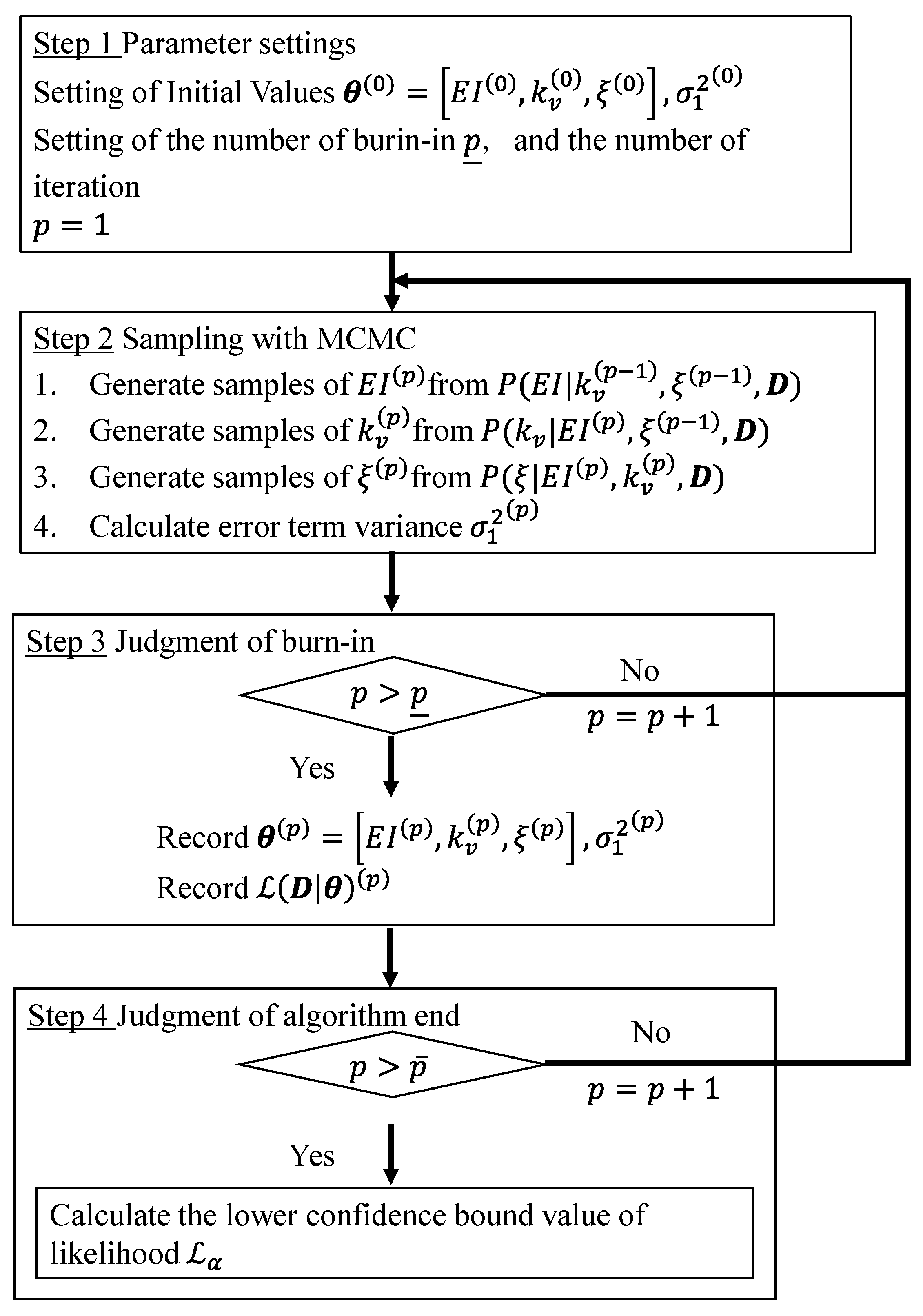
2.3. Structural Model Updating Method

Bayesian estimation is a methodology for estimating an occurrence model of an event from observed data. The development of numerical estimation methods, such as MCMC, has promoted the utilization of Bayesian estimation in SMU in recent years (Reference [17] reports a detailed theoretical background of the method). In formulating the Bayesian SMU, the maximum acceleration calculated by Equation (17) is expressed as the following function:

$$a_{\mathit{num}}\left(EI, k_v,\xi ,v\right).$$

(18)

Regarding the structural model $a_{\mathit{num}}\left(EI, k_v,\xi ,v\right)$ that has been converted into a function, the unknown parameter vector is expressed as $\mathit{\theta }=\left[\mathit{E}\mathit{I},{\mathit{k}}_{\mathit{v}},\mathit{\xi }\right]$. As $\mathit{m}$ can be used as a design value, it is assumed to be a known parameter in this study. Additionally, the measurement dataset of the maximum acceleration during the passing of trains, which are observed events, is defined as $\mathit{D}=\left({\tilde{y}}_1,{\tilde{y}}_2,\cdots ,{\tilde{y}}_{Sn}\right)$, and the corresponding measurement dataset of the train speed is defined as $\mathit{V}=\left({\tilde{v}}_1,{\tilde{v}}_2,\cdots ,{\tilde{v}}_{Sn}\right)$. Notably, $\mathit{V}$ is an explanatory variable. In this case, Bayes’ theorem holds that the occurrence probability of the parameter vector $\mathit{\theta }$ given the measurement dataset $\mathit{D}$ is given by Equation (19).

$$\mathrm{P}\left(\mathit{\theta }|\mathit{D}\right)\propto \mathcal{L}\left(\mathit{D}|\mathit{\theta }\right)\mathrm{P}\left(\mathit{\theta }\right),$$

(19)

where $\mathcal{L}\left(\mathit{D}|\mathit{\theta }\right)$ is the likelihood function, $\mathrm{P}\left(\mathit{\theta }\right)$ is the prior distribution, $\mathrm{P}\left(\mathit{\theta }|\mathit{D}\right)$ is the posterior distribution, and $\propto$ represents a proportional relationship. Here, $\mathrm{P}\left(\mathit{\theta }|\mathit{D}\right)$ is the parameter distribution to be estimated. Therefore, by setting $\mathcal{L}\left(\mathit{D}|\mathit{\theta }\right)$ and $\mathrm{P}\left(\mathit{\theta }\right)$, $\mathrm{P}\left(\mathit{\theta }|\mathit{D}\right)$ can be estimated.

The likelihood $\mathcal{L}\left(\mathit{D}|\mathit{\theta }\right)$ is the probability of the simultaneous occurrence of data $\mathit{D}$ when the parameter $\mathit{\theta }$ is given. It is assumed that the error between the output (maximum acceleration) of the model with the parameter θ that best matches the data and the observed maximum acceleration follows a normal distribution. In this case, $\mathcal{L}\left(\mathit{D}|\mathit{\theta }\right)$ can be defined using Equation (20), assuming that the expectation and variance of the distribution of the measured maximum acceleration $\mathit{D}$ are expressed by the maximum acceleration $a_{num}\left(\mathit{\theta },V\right)$ calculated by a structural model with appropriate parameter values, as well as the observation error ${\sigma }^2$. $\mathit{N}\left(Exp,Var\right)$ is a normal distribution with the expectation $\mathrm{E}\mathrm{x}\mathrm{p}$ and variance $\mathrm{V}\mathrm{a}\mathrm{r}$.

$$\mathcal{L}\left(\mathit{D}|\mathit{\theta }\right)={\prod }_{\mathit{s}\mathit{n}=1}^{\mathit{S}\mathit{n}}\mathit{N}\left({\tilde{y}}_{sn}-a_{num}\left(\mathit{\theta },{\tilde{\mathit{v}}}_{\mathit{s}\mathit{n}}\right),{\sigma }^2\right).$$

(20)

Assuming an unconditional $\mathrm{P}\left(\mathit{\theta }\right)$ was set for $\mathrm{P}\left(\mathit{\theta }\right)$, an estimated value $\widehat{\mathit{\theta }}$ that is determined entirely from the data can be obtained. In this study, relatively loose constraints were introduced only to the $\mathrm{P}\left(\mathit{\theta }\right)$ of $k_v$ ($\mathrm{P}\left(k_v\right)$) to investigate the effect of the number of samples $Sn$, setting the expected value to the design value (5 GN/m) and the standard deviation to half the design value (2.5 GN/m); moreover, the other $\mathrm{P}\left(\mathit{\theta }\right)$ values ($\mathrm{P}\left(\mathit{E}\mathit{I}\right)$ and $\mathrm{P}\left(\mathit{\xi }\right)$) of $\mathit{E}\mathit{I}$ and $\mathit{\xi }$ were set to uniform distributions with a domain from 0 to infinity. Wide prior distributions are used to accurately assess the effect of sample size on the posterior distribution. MCMC is used to numerically approximate Equation (21), which is obtained by substituting the above likelihood and prior distribution into Equation (19).

$$\mathrm{P}\left(\mathit{\theta }|\mathit{D}\right)\propto \mathrm{P}\left(k_v\right)\mathrm{P}\left(\mathit{E}\mathit{I}\right)\mathrm{P}\left(\mathit{\xi }\right){\prod }_{\mathit{s}\mathit{n}=1}^{\mathit{S}\mathit{n}}\mathit{N}\left({\tilde{y}}_{sn}-F\left(\mathit{\theta },{\tilde{\mathit{v}}}_{\mathit{s}\mathit{n}}\right),{\sigma }^2\right).$$

(21)

When the influence of the prior distribution is disregarded, the effect of sample size reduces to the problem of evaluating how $\mathit{S}\mathit{n}$ influences $\prod _{\mathit{s}\mathit{n}=1}^{\mathit{S}\mathit{n}}\mathit{N}\left({\tilde{y}}_{sn}-F\left(\mathit{\theta },{\tilde{\mathit{v}}}_{\mathit{s}\mathit{n}}\right),{\sigma }^2\right)$. More specifically, it can be characterized by the relationship between $\mathit{S}\mathit{n}$ and ${\sigma }^2$. Given that ${\sigma }^2=\mathit{E}\left\{{\left({\tilde{y}}_{sn}-F\right)}^2\right\}=\prod _{\mathit{s}\mathit{n}=1}^{\mathit{S}\mathit{n}}{\left({\tilde{y}}_{sn}-F\right)}^2/S_n$, if the squared error ${\left({\tilde{y}}_{sn}-F\right)}^2$ of each sample is identical across all samples—which is approximately the case when the model $\mathit{F}$ accurately represents the observed data—then the spread of the posterior distribution decreases as $S_n$ increases, due to the resulting increase in the aggregate distribution. However, if the number of samples is insufficient to adequately estimate the parameters of $\mathit{F}$, the squared errors ${\left({\tilde{y}}_{sn}-F\right)}^2$ associated with individual samples tend to exhibit significant bias. In such cases, the relationship between the number of samples and the variability in the posterior distribution becomes more complex. The aim of this study is to empirically investigate this issue using actual measurement data.

Figure 7 shows the estimation flow of $\mathrm{P}\left(\mathit{\theta }|\mathit{D}\right)$ using MCMC. In this study, $\mathrm{P}\left(\mathit{\theta }|\mathit{D}\right)$ was first divided, as $\mathrm{P}\left(\mathit{\theta }=\left[\mathit{E}\mathit{I},{\mathit{k}}_{\mathit{v}},\mathit{\xi }\right]|\mathit{D}\right)$, which cannot be directly generated (sampled), into a fully conditional $\mathrm{P}\left(\mathit{\theta }|\mathit{D}\right)$ ($\mathrm{P}\left(\mathit{E}\mathit{I}|k_v,\mathit{\xi },\mathit{D}\right)$, $\mathrm{P}\left(k_v|\mathit{E}\mathit{I},\mathit{\xi },\mathit{D}\right)$, and $\mathrm{P}\left(\mathit{\xi }|\mathit{E}\mathit{I},k_v,\mathit{D}\right)$) for each unknown parameter. Thereafter, $\mathrm{P}\left(\mathit{\theta }|\mathit{D}\right)$ was obtained using the Gibbs sampling approach, which replaces the sampling from each fully conditional $\mathrm{P}\left(\mathit{\theta }|\mathit{D}\right)$. However, as each fully conditional $\mathrm{P}\left(\mathit{\theta }|\mathit{D}\right)$ cannot be directly generated as random numbers, the random-walk Metropolis–Hastings (RW-MH) algorithm was used to sample from each fully conditional $\mathrm{P}\left(\mathit{\theta }|\mathit{D}\right)$. The RW-MH algorithm gradually converges to the fully conditional $\mathrm{P}\left(\mathit{\theta }|\mathit{D}\right)$ by sampling via an acceptance and rejection process; the convergence process is called burn-in. In the RW-MH algorithm, random numbers are first generated from a normal distribution with a mean 0 and variance ${\mathit{\nu }}^2$ based on the sample taken in the previous ($\mathit{p}-1$)th sample to obtain the $\mathit{p}$th sample. Further, the ratio of the likelihoods for the ($\mathit{p}-1$)th and $\mathit{p}$th samples determines whether the generated random numbers follow the full conditional $\mathrm{P}\left(\mathit{\theta }|\mathit{D}\right)$. Here, for the $\mathit{p}$th sampling, the $\mathit{E}\mathit{I}$ sample $\mathit{E}{I}^{\left(p\right)}$ was sampled from $\mathrm{P}\left(\mathit{E}\mathit{I}|k_v^{\left(p-1\right)},{\xi }^{(p-1)},\mathit{D}\right)$, $k_v^{\left(p\right)}$ of the bearing stiffness was sampled from $\mathrm{P}\left(k_v|\mathit{E}{I}^{\left(p\right)},{\xi }^{(p-1)},\mathit{D}\right)$, and $\mathit{\xi }$ (${\xi }^{\left(p\right)}$) was sampled from $\mathrm{P}\left(\mathit{\xi }|\mathit{E}{I}^{\left(p\right)},k_v^{\left(p\right)},\mathit{D}\right)$ in sequence using the RW-MH method. This calculation was repeated, and the samples after sampling number $\overline{p}$, which was sufficiently larger than the burn-in, were recorded as samples from $\mathrm{P}\left(\mathit{\theta }|\mathit{D}\right)$. The sampling continued after sampling number $\overline{p}$, and the calculation ended with the sampling of number $\underset{\_}{p}$ from the burn-in. The recorded samples ${\mathit{\theta }}^{\overline{\mathit{p}}:\underset{\_}{\mathit{p}}}=[{\mathit{\theta }}^{\left(\overline{\mathit{p}}+1\right)},\dots ,{\mathit{\theta }}^{\left(\underset{\_}{\mathit{p}}\right)}]$ from $\overline{p}+1$ to $\underset{\_}{p}$ were considered samples from $\mathrm{P}\left(\mathit{\theta }|\mathit{D}\right)$; thus, the estimated values and uncertainties were obtained by calculating their statistics (the expected value and confidence interval (CI)).

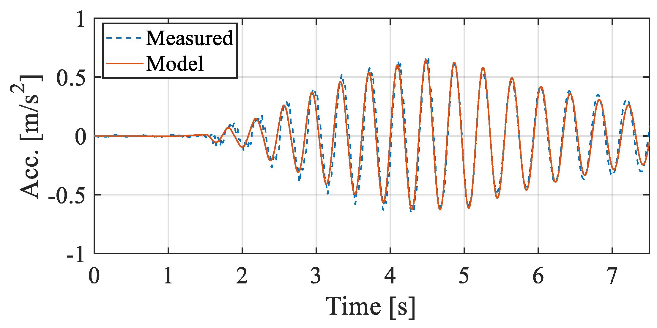
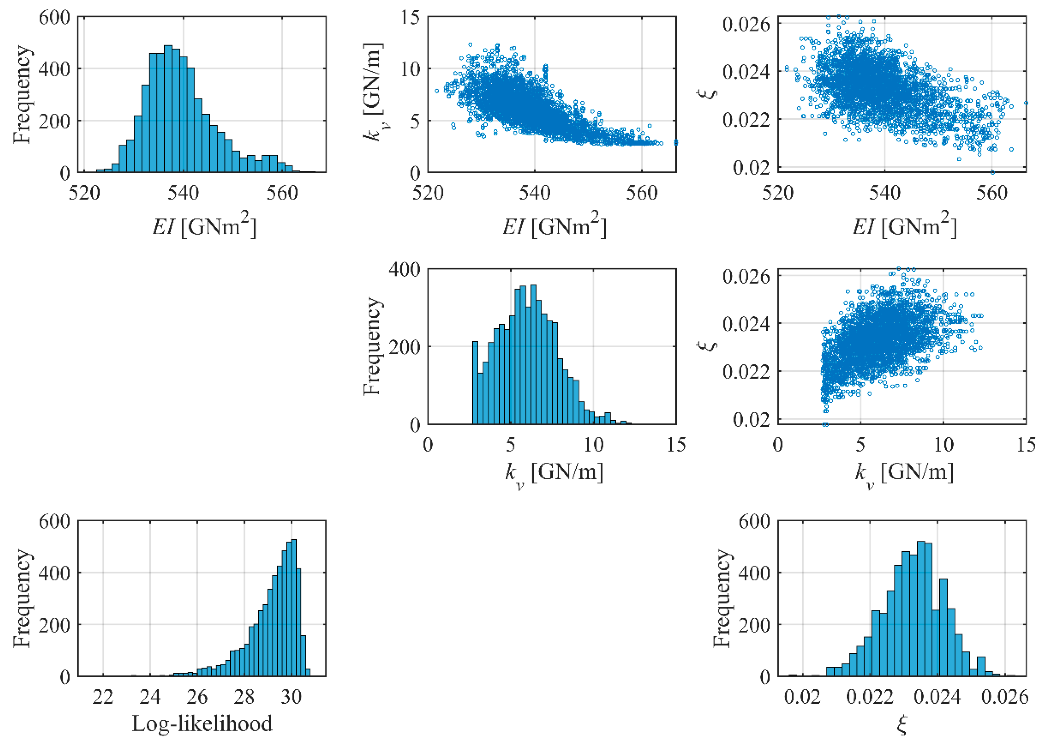
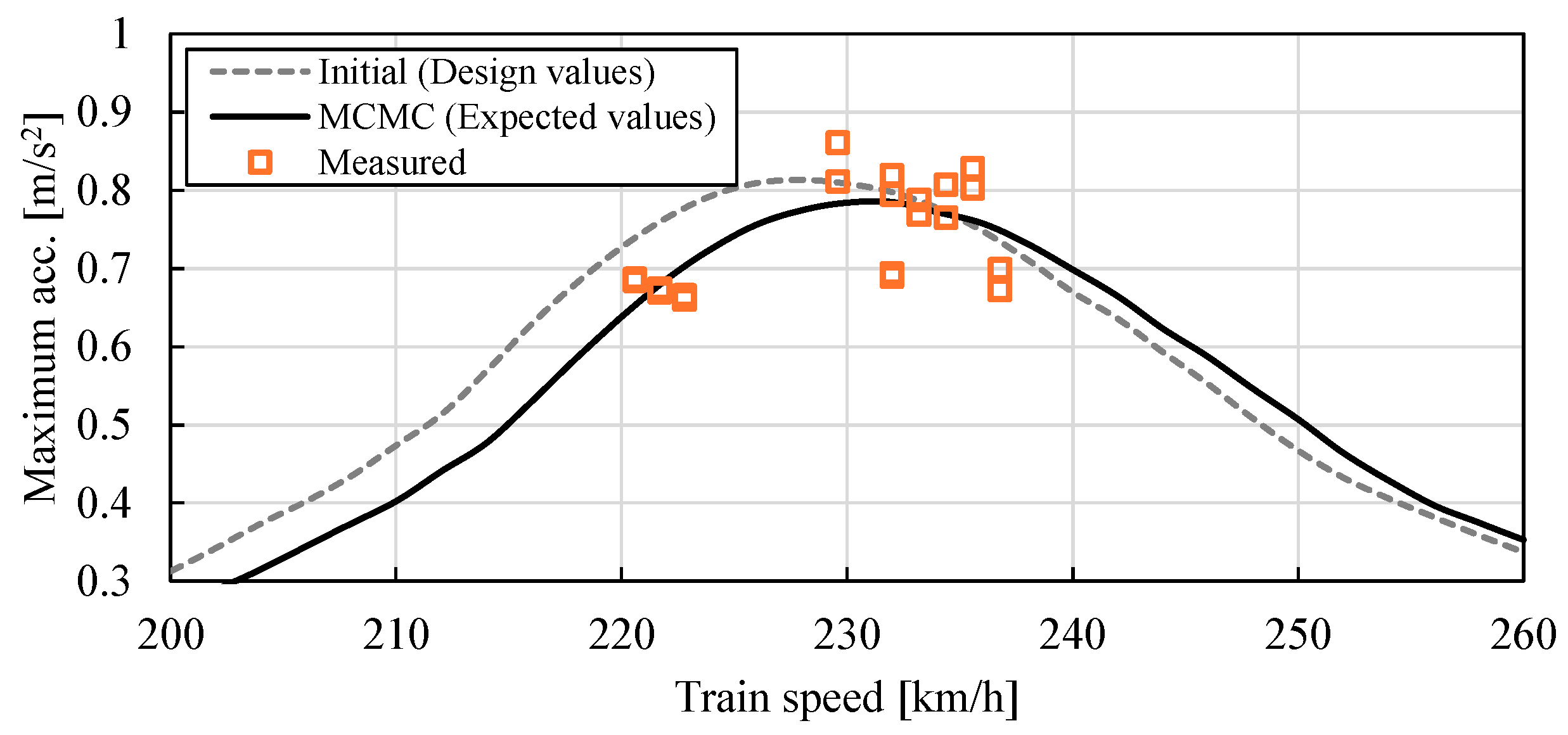
3. Estimation Results for All the Data

Figure 8 shows $\mathrm{P}\left(\mathit{\theta }|\mathit{D}\right)$ and the log-likelihood distribution of the unknown parameters estimated using the method described in Section 2.3 based on the maximum acceleration (total 20 samples) measured by G3 and G4 during the passing of the trains. In the MCMC method, the total number of samplings was 7000, the burn-in was 2000, and samples 2001–7000 were taken as the samples from $\mathrm{P}\left(\mathit{\theta }|\mathit{D}\right)$. Employing the maximum acceleration of the 20 samples, a unimodal $\mathrm{P}\left(\mathit{\theta }|\mathit{D}\right)$ was estimated for each parameter. The expected value (6.5 GN/m) and 95% CI (3.5–9.9 GN/m) of $k_v$ were almost the same, and there was a relatively large variance. Conversely, the 95% CI of $\mathit{E}\mathit{I}$ was less than 5% of the expected value (expected value: 540 GNm², 95% CI 530–552 GNm²); it could be estimated with high accuracy and slight uncertainty. The 95% CI for $\mathit{\xi }$ was approximately 10% of the expected value (expected value: 0.022, 95% CI 0.021–0.024), which was not a low accuracy level.

Figure 9 shows a comparison between the maximum acceleration calculated using the expected values of $\mathrm{P}\left(\mathit{\theta }|\mathit{D}\right)$ of each estimated parameter and the measured maximum acceleration. The Bayesian SMU-estimated results accurately expressed the trends in the measured results compared to those calculated using design-based initial values. From the foregoing, at least for the test bridge, although a large uncertainty existed in $k_v$, $\mathit{E}\mathit{I}$ and $\mathit{\xi }$ could be accurately estimated by updating the structural model using the 20 maximum-acceleration samples, making it possible to obtain a structural model that accurately expresses the maximum acceleration of the actual bridge. It should be noted that the upper bound of the maximum acceleration might appear to be obtainable by using the lower bounds of the posterior distributions for each parameter. However, as shown in Figure 8, correlations exist within the joint posterior distribution of the parameters. Consequently, the probability that, for example, both the damping ratio and the flexural stiffness simultaneously attain their respective 5% lower bounds does not correspond to the 5% lower bound of the peak acceleration. This issue is discussed in detail in [26], and interested readers are referred to that reference for further information. These results were the prerequisite for the sensitivity investigation of the sample size below.

4. Discussion About Sample Size

4.1. Effect of the Number of Accelerometers

Figure 10 shows $\mathrm{P}\left(\mathit{\theta }|\mathit{D}\right)$s estimated using the maximum-acceleration data (10 samples each) obtained from only G3 or G4, along with the results for all the samples. The expected value for EI did not change significantly, although the tail of $\mathrm{P}\left(\mathit{\theta }|\mathit{D}\right)s$ estimated using only G4 spread upward. When one accelerometer was not used, the tail of the $\mathit{\xi }$ distribution spread, and the expected value shifted by approximately 15%. As shown in Figure 3, the slightly higher peak acceleration of sensor G4 at 230 km/h is considered to have resulted in a decrease in the modal damping ratio. On the other hand, since the peak accelerations of the two sensors are nearly identical around 220 km/h, it is inferred that the broader distribution of the damping ratio estimated using only sensor G4 serves to compensate for this discrepancy. Additionally, the $k_v$ of the support exhibited characteristics, such as a shift in the expected $\mathrm{P}\left(\mathit{\theta }|\mathit{D}\right)$ or the appearance of another small peak, all of which were the effects of the decrease in the number of observation samples obtained using only the data from one accelerometer. Conversely, the accuracy of the estimation results might be improved by increasing the number of samples even if the accelerometers differed. However, the conditions under which combining the data from different accelerometers effectively improved the accuracy were unclear. Although it was effective for the test bridge in this study, future studies should explore detailed investigations on other bridges and effective locations.

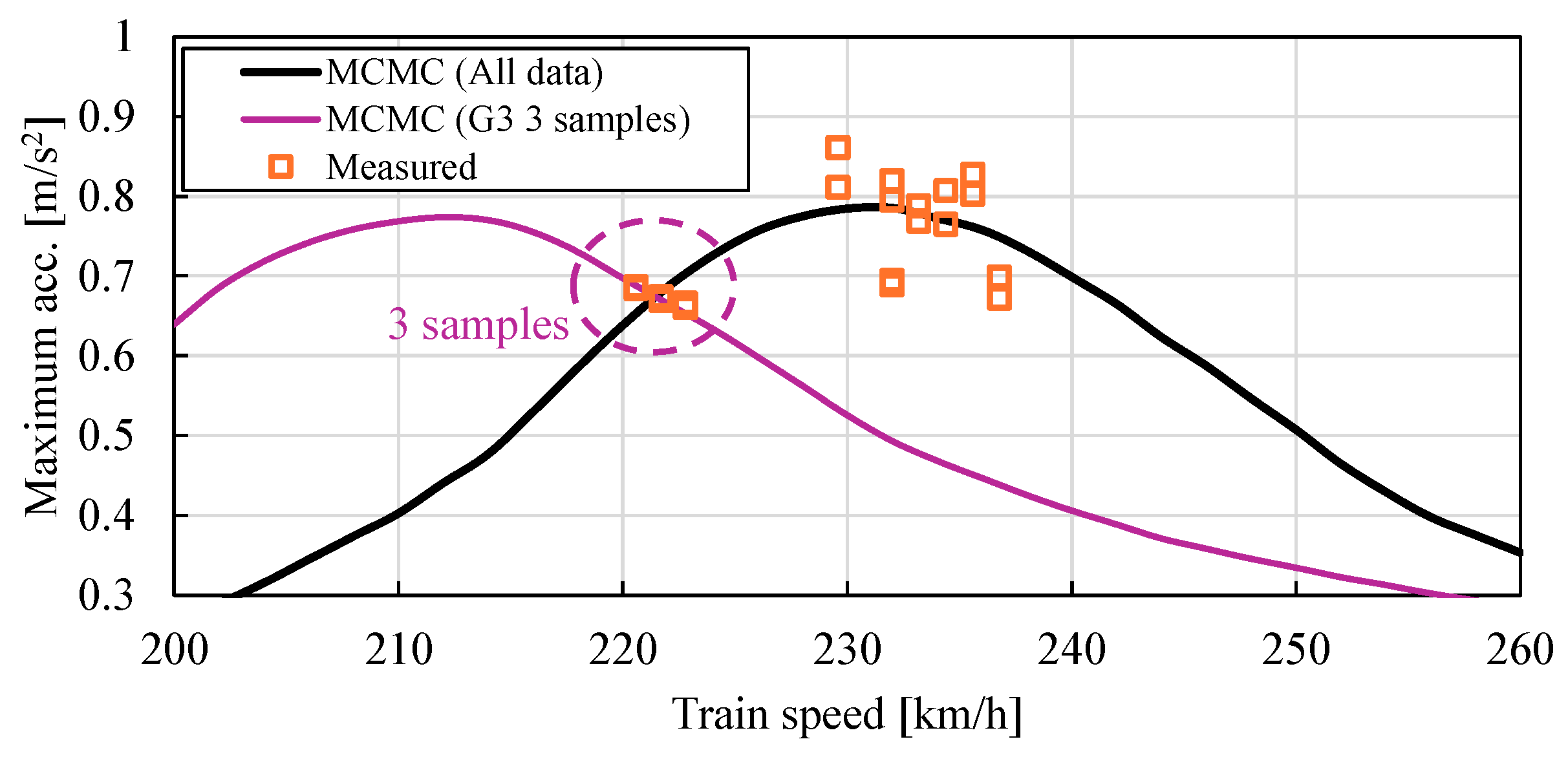
4.2. Effect of the Observation-Sample Number

Figure 11 shows the results of $\mathrm{P}\left(\mathit{\theta }|\mathit{D}\right)s$ estimated using G3 with several maximum-acceleration sample numbers. The results for all the data and 10 samples are the same as in Figure 8. The cases with sample numbers of three and five were selected from the low-speed side of Figure 3. Further, the tails of $\mathrm{P}\left(\mathit{\theta }|\mathit{D}\right)s$ of $\mathit{E}\mathit{I}$ and $\mathit{\xi }$ widened significantly as the number of samples was reduced to five. Additionally, the local solutions around 1 GN/m dominated the $k_v$ of the bearing. Furthermore, as the number of samples reduced to three, the tails of $\mathrm{P}\left(\mathit{\theta }|\mathit{D}\right)s$ of all the parameters did not widen; they converged to values different from the estimation results when all the samples were used (this is the result of being heavily influenced by local solutions). This result does not necessarily correlate with the understanding of the behavior of $\mathrm{P}\left(\mathit{\theta }|\mathit{D}\right)$ as the number of samples increased in the existing Bayesian SMU. It is established that the variance in $\mathrm{P}\left(\mathit{\theta }|\mathit{D}\right)$ decreases and the accuracy improves as the number of samples increases in Bayesian updating [19]. Conversely, an extremely small number of samples (three in this study) does not significantly change the width of the tail of $\mathrm{P}\left(\mathit{\theta }|\mathit{D}\right)s$ from when all the samples were used because the distribution converges to a local solution. Figure 12 shows the maximum-acceleration calculated using the expected values of $\mathrm{P}\left(\mathit{\theta }|\mathit{D}\right)$ of each estimated parameter in the case of the three samples. The figure indicates that the three samples’ results clearly converge to a local solution. Although the accuracy indeed improves with the increasing number of samples, the tail width of $\mathrm{P}\left(\mathit{\theta }|\mathit{D}\right)s$ does not necessarily decrease with the increasing number of samples. When a local solution was obtained, there were cases where the tail width increased once as the number of samples increased, after which it decreased as the distribution converged to the optimal solution. This tendency might depend on the number of samples and data quality. Therefore, the case in which the number of samples was three, and the data from the resonance range (230–235 km/h) was used instead of the non-resonance range (train speed: 220–225 km/h), employed in this study was examined in Section 4.3.

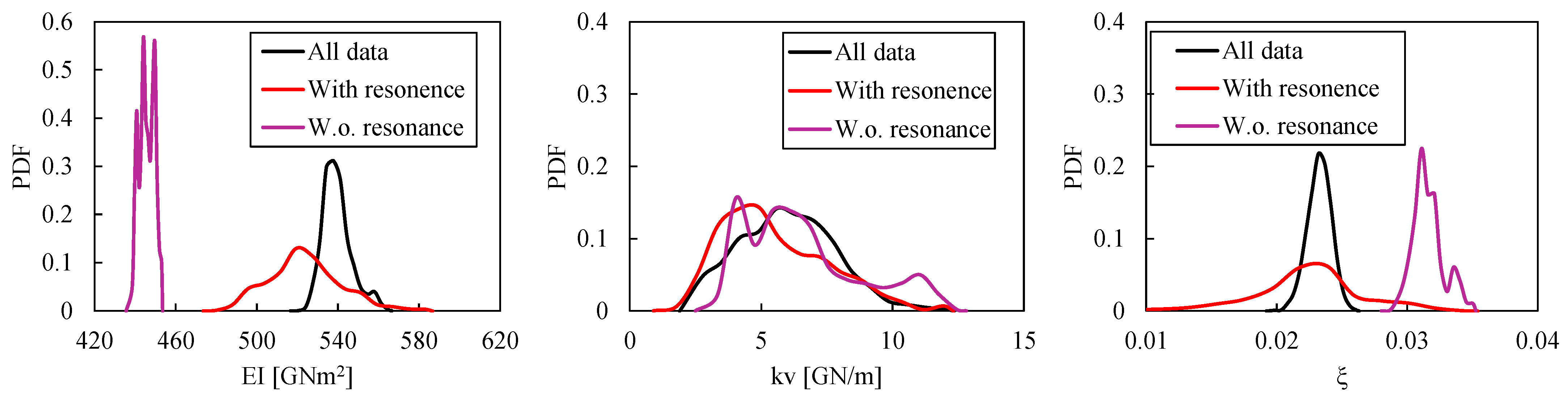
4.3. Effect of the Observation Samples of the Resonant Region

Figure 13 shows a comparison of the results for G3 when the three maximum-acceleration samples used for the estimation included and did not include the data from the resonance region. The results of $\mathrm{P}\left(\mathit{\theta }|\mathit{D}\right)$ estimated by the number of samples are shown. The estimation results obtained with all the data in Figure 8 are also shown for comparison. When the three maximum-acceleration samples included data from the resonance region (230–235 km/h), the convergence to a local solution differed significantly from the expected value for all the data, especially for EI and $\mathit{\xi }$, which disappeared. Rather, as is well known, the tail of $\mathrm{P}\left(\mathit{\theta }|\mathit{D}\right)s$ tended to widen much more than in the case of all the data. This result indicated that the samples from the resonance region containing many dynamic responses were necessary for the accurate estimation of the Bayesian SMU of HSR bridges. The observation data from the resonance region might be high-quality data for the Bayesian SMU of HSR bridges. This is due to the fact that data within the resonance region contain a greater influence of the amplified dynamic response of the bridge. In particular, the effect of the modal damping ratio $\mathit{\xi }$ becomes more pronounced under conditions where dynamic responses occur. Conversely, quasi-static bridge responses outside the resonance region are minimally affected by the modal damping ratio, which likely explains the reduced accuracy of the SMU when data excluding the resonance region are used. For this test bridge, assuming high-quality samples from the resonance region could be obtained, $\mathit{E}\mathit{I}$ and $\mathit{\xi }$ could be updated with the same accuracy as the case of five samples that do not include the resonance region (Figure 10), even with only three samples.

4.4. Perspectives on Practical Application

The results of this study clarified that the observation data in the resonance region of the HSR bridge were high-quality data for the Bayesian SMU. Assuming the data in the resonance region could be observed, a higher-accuracy result would be obtained with fewer samples than when other observation data are used. Thus, the time and effort of on-site measurements could be reduced. Conversely, determining whether the test bridge resonated before measuring the acceleration at the site is practically challenging. However, methodologies for determining the resonance state of the bridge from data, such as vehicle acceleration or track geometry obtained on the running train, have been developed in recent years [27,28]. By exploring such information, it is possible to predict whether each bridge resonates and estimate the resonance speed when resonance occurs before field measurements. In resonant bridges, the bridge dynamic response gradually increases as the train passes over it. As a result, the dynamic response excited during the passage of the trailing car is significantly greater than that during the passage of the leading car. These methods detect resonant bridges by quantifying this characteristic behavior as differences in track geometry or car body acceleration measured at the positions of the leading and trailing cars. This facilitates the temporary measurement of the response during the traveling of the train at the predicted speed. The test bridge in this study is the same one that was detected as a resonant bridge by the drive-by method proposed in Reference [27]. A structural model is required to determine the need for repairs, select a repair method, and predict the repair effect. The SMU in this study responds precisely to such practical requirements in practice. Moreover, the findings and discussions presented in this study offer an academic contribution in terms of achieving a high-accuracy Bayesian SMU with a smaller number of samples by emphasizing the importance of data quality. Specifically, the results demonstrate that samples obtained within the resonance region constitute high-quality data and are particularly valuable for the estimation of the key parameters of high-speed railway bridges, such as bending stiffness and modal damping ratio. The findings from this study have academic and practical implications; they can help reduce the burden of the on-site measurements required to obtain structural models with the required accuracy.

5. Conclusions

In this study, the effect of the number of samples of the maximum-acceleration data measured on-site on $\mathrm{P}\left(\mathit{\theta }|\mathit{D}\right)s$ obtained by the Bayesian SMU was investigated using an actual HSR bridge. A PC box girder bridge spanning approximately 50 m on a Japanese HSR was the focus of the study, and $\mathit{E}\mathit{I}$, $k_v$, and $\mathit{\xi }$ were estimated using Bayesian SMU from the maximum acceleration when multiple trains traveled on the bridge. Additionally, the effects of the number of acceleration samples employed for SMU, as well as the effects of the quality of the samples, such as whether they included the resonance region, were empirically validated. The findings revealed that when converging to a local solution in the test bridge, the tail of $\mathrm{P}\left(\mathit{\theta }|\mathit{D}\right)s$ may become narrow, even though the number of samples is small. As the number of samples increases, the tail of $\mathrm{P}\left(\mathit{\theta }|\mathit{D}\right)s$ may widen significantly once, after which it will converge to the global optimum value. When samples from the resonance region were included, the convergence to a local solution was avoidable even with three samples, and the estimation accuracy was equivalent to that obtained with five samples from the non-resonance region.

The main limitations of this study are as follows: First, although the findings are based on valuable results obtained from an actual bridge, only one bridge was considered. The results from studies of other bridge types and span lengths can be combined to generalize the number of samples required and develop a framework and methodology for quantitatively evaluating the data quality. Additionally, maximum bridge acceleration was employed as the observed data, although bridge displacements and acceleration waveforms might also suffice. Therefore, investigating the effects of the type and format of the observed data used to update the Bayesian structural model would be valuable [29]. When using the full waveform directly, it may be possible to avoid the influence of local optima observed in this study. However, this approach requires a precise time synchronization between the simulated and measured waveforms, which must be addressed in the future.

References

1. Frýba, L. Vibration of Solids and Structures Under Moving Loads; Springer Nature: Dordrecht, The Netherlands, 2013; Volume 1. [Google Scholar] [CrossRef]
2. Ju, S.H.; Lin, H.T. Resonance characteristics of high-speed trains passing simply supported bridges. J. Sound Vib. 2003, 267, 1127–1141. [Google Scholar] [CrossRef]
3. Sogabe, M.; Matsumoto, N.; Kanamori, M.; Sato, T.; Wakui, H. Impact factors of concrete girders coping with train speed-up. Q. Rep. RTRI 2005, 46, 46–52. [Google Scholar] [CrossRef]
4. He, X.; Wu, T.; Zou, Y.; Chen, Y.F.; Guo, H.; Yu, Z. Recent developments of high-speed railway bridges in China. Struct. Infrastruct. Eng. 2017, 13, 1584–1595. [Google Scholar] [CrossRef]
5. Ferreira, G.; Montenegro, P.; Andersson, A.; Henriques, A.A.; Karoumi, R.; Calçada, R. Critical analysis of the current Eurocode deck acceleration limit for evaluating running safety in ballastless railway bridges. Eng. Struct. 2024, 312, 118127. [Google Scholar] [CrossRef]
6. Sogabe, M.; Furukawa, A.; Shimomura, T.; Iida, T.; Matsumoto, N.; Wakui, H. Deflection limits of structures for train speed-up. Q. Rep. RTRI 2005, 46, 130–136. [Google Scholar] [CrossRef]
7. Frýba, L. A rough assessment of railway bridges for high speed trains. Eng. Struct. 2001, 23, 548–556. [Google Scholar] [CrossRef]
8. Matsuoka, K.; Tokunaga, M.; Kaito, K. Bayesian estimation of instantaneous frequency reduction on cracked concrete railway bridges under high-speed train passage. Mech. Syst. Signal Process. 2021, 161, 107944. [Google Scholar] [CrossRef]
9. Matsuoka, K.; Collina, A.; Somaschini, C.; Sogabe, M. Influence of local deck vibrations on the evaluation of the maximum acceleration of a steel-concrete composite bridge for a high-speed railway. Eng. Struct. 2019, 200, 109736. [Google Scholar] [CrossRef]
10. Ülker-Kaustell, M.; Karoumi, R. Influence of non-linear stiffness and damping on the train-bridge resonance of a simply supported railway bridge. Eng. Struct. 2012, 41, 350–355. [Google Scholar] [CrossRef]
11. Li, J.; Su, M. The resonant vibration for a simply supported girder bridge under high-speed trains. J. Sound Vib. 1999, 224, 897–915. [Google Scholar] [CrossRef]
12. Matsuoka, K.; Kaito, K.; Sogabe, M. Bayesian time–frequency analysis of the vehicle–bridge dynamic interaction effect on simple-supported resonant railway bridges. Mech. Syst. Signal Process. 2020, 135, 106373. [Google Scholar] [CrossRef]
13. Ubertini, F.; Gentile, C.; Materazzi, A.L. Automated modal identification in operational conditions and its application to bridges. Eng. Struct. 2013, 46, 264–278. [Google Scholar] [CrossRef]
14. Ribeiro, D.; Calçada, R.; Delgado, R.; Brehm, M.; Zabel, V. Finite element model updating of a bowstring-arch railway bridge based on experimental modal parameters. Eng. Struct. 2012, 40, 413–435. [Google Scholar] [CrossRef]
15. Matsuoka, K.; Shinozaki, S.; Kaito, K. Structural model update considering uncertainty and reliability assessment of strengthening effect: Application to additional supporting strengthening of a high-speed railway bridge. J. Jpn. Soc. Civ. Eng. Ser. A1 2020, 76, 560–579. [Google Scholar] [CrossRef]
16. Mottershead, J.E.; Friswell, M.I. Model updating in structural dynamics: A survey. J. Sound Vib. 1993, 167, 347–375. [Google Scholar] [CrossRef]
17. Beck, J.L.; Katafygiotis, L.S. Updating models and their uncertainties. I: Bayesian statistical framework. J. Eng. Mech. 1998, 124, 455–461. [Google Scholar] [CrossRef]
18. Simoen, E.; De Roeck, G.; Lombaert, G. Dealing with uncertainty in model updating for damage assessment: A review. Mech. Syst. Signal Process. 2015, 56, 123–149. [Google Scholar] [CrossRef]
19. Ierimonti, L.; Cavalagli, N.; Venanzi, I.; García-Macías, E.; Ubertini, F. A transfer Bayesian learning methodology for structural health monitoring of monumental structures. Eng. Struct. 2021, 247, 113089. [Google Scholar] [CrossRef]
20. Yu, X.; Li, X.; Bai, Y. Evaluating maximum inter-story drift ratios of building structures using time-varying models and Bayesian filters. Soil. Dyn. Earthq. Eng. 2022, 162, 107496. [Google Scholar] [CrossRef]
21. Kammouh, O.; Gardoni, P.; Cimellaro, G.P. Probabilistic framework to evaluate the resilience of engineering systems using Bayesian and dynamic Bayesian networks. Reliab. Eng. Syst. Saf. 2020, 198, 106813. [Google Scholar] [CrossRef]
22. Vanik, M.W.; Beck, J.L.; Au, S.K. Bayesian probabilistic approach to structural health monitoring. J. Eng. Mech. 2000, 126, 738–745. [Google Scholar] [CrossRef]
23. Johansson, C.; Pacoste, C.; Karoumi, R. Closed-form solution for the mode superposition analysis of the vibration in multi-span beam bridges caused by concentrated moving loads. Comput. Struct. 2013, 119, 85–94. [Google Scholar] [CrossRef]
24. Mao, L.; Lu, Y. Critical speed and resonance criteria of railway bridge response to moving trains. J. Bridge Eng. 2013, 18, 131–141. [Google Scholar] [CrossRef]
25. Nakada, M.; Matsuoka, K. Closed form solution of multipoint support beam under moving load for simple calculation of dynamic response of railway continuous bridges. Trans. Jpn. Soc. Civ. Eng. 2023, 79, 22-15052. [Google Scholar] [CrossRef]
26. Yotsui, H.; Matsuoka, K.; Kaito, K. Dual sampling method for evaluating uncertainty when updating a Bayesian estimation model of a high-speed railway bridge. Reliab. Eng. Syst. Saf. 2025, 259, 110901. [Google Scholar] [CrossRef]
27. Matsuoka, K.; Tanaka, H.; Kawasaki, K.; Somaschini, C.; Collina, A. Drive-by methodology to identify resonant bridges using track irregularity measured by high-speed trains. Mech. Syst. Signal Process. 2021, 158, 107667. [Google Scholar] [CrossRef]
28. Matsuoka, K.; Tanaka, H. Drive-by deflection estimation method for simple support bridges based on track irregularities measured on a traveling train. Mech. Syst. Signal Process. 2023, 182, 109549. [Google Scholar] [CrossRef]
29. Ereiz, S.; Duvnjak, I.; Jiménez-Alonso, J.F. Review of finite element model updating methods for structural applications. Structures 2022, 41, 684–723. [Google Scholar] [CrossRef]
Figure 1. Cross-section of the test bridge.
Infrastructures 10 00108 g001
Figure 2. Acceleration spectrum of G3 during the passing of a train (235 km/h).
Infrastructures 10 00108 g002
Figure 3. Relationship between the maximum acceleration and the train speed (30 Hz LPF).
Infrastructures 10 00108 g003
Figure 4. Data used in each case for all data.
Infrastructures 10 00108 g004
Figure 5. Modeling of the bridge and traveling train as (a) an elastic-supported beam and (b) moving loads.
Infrastructures 10 00108 g005
Figure 6. Comparison of the calculated and measured acceleration responses (30 Hz LPF).
Infrastructures 10 00108 g006
Figure 7. Parameter-estimation algorithm using the MCMC method.
Infrastructures 10 00108 g007
Figure 8. P θ D s obtained by sampling using the MCMC method (all data: 20 samples).
Infrastructures 10 00108 g008
Figure 9. Comparison between the calculated and measured maximum acceleration.
Infrastructures 10 00108 g009
Figure 10. Comparison of P θ D s estimated using only the G3 or G4 samples.
Infrastructures 10 00108 g010
Figure 11. Comparison of P θ D s estimated using various sample numbers.
Infrastructures 10 00108 g011
Figure 12. Comparison between the maximum accelerations calculated using 3 and all samples.
Infrastructures 10 00108 g012
Figure 13. Effect of the presence or absence of resonance-region samples on the estimation results of P θ D (sample number: 3).
Infrastructures 10 00108 g013