1. Introduction
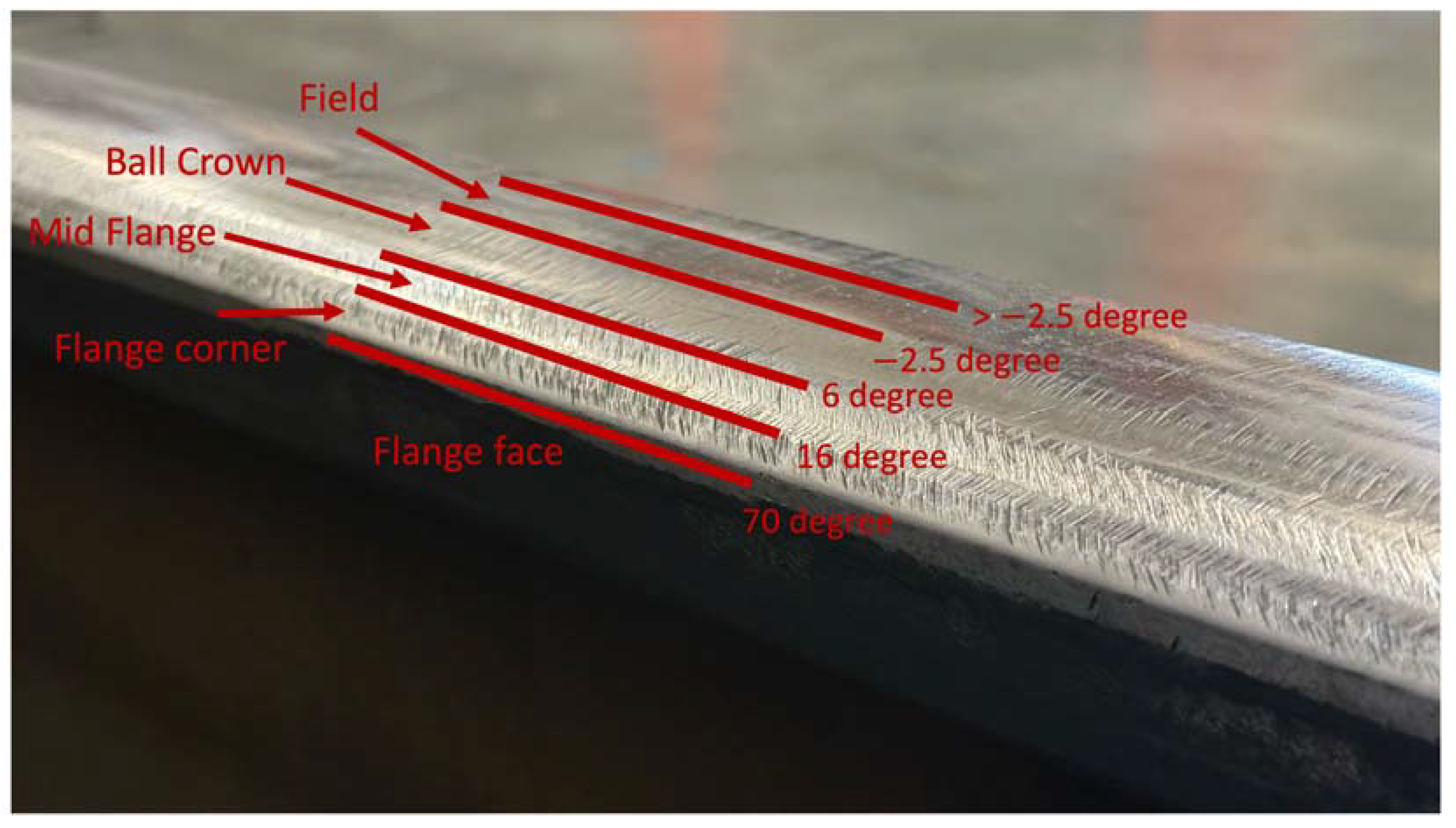
Proper lubrication of rail surfaces in curved tracks is necessary in the railway industry to minimize rail wear while ensuring safe and efficient operations. Specifically, flange-face lubrication is vital for reducing wear between the wheel and the rail’s flange face and corner in curves [
1,
2] (
Figure 1). Flange lubrication is particularly critical in tight curves, where significant lateral forces exist between the wheel and rail. Furthermore, it also contributes to reducing the risk of wheel-climb derailments [
1,
3,
4]. When trains navigate a curve, the outer rail to the curve, commonly called the “high rail”, experiences more wear due to the lateral forces and wheel flange contact. Proper flange-face lubrication on the high rail significantly reduces wear, contributing to longer wheel and rail life and lower maintenance costs [
5]. It also reduces rolling contact fatigue at the rail head [
6], decreases wheel squeal [
7], and reduces fuel consumption [
8,
9]. While the inner rail, or “low rail”, also experiences significant wear, it is primarily due to friction from wheel tread contact rather than flange contact. This wear is caused by creep forces, friction, and the redistribution of load as the train negotiates the curve [
10].
Grease is applied to the flange-face profile in curves with the help of wayside applicators [
11]. The grease is squirted on the rail as a train approaches and then carried along the track by the rotating train wheels. The grease applicators are placed strategically before curves with attendant high-wear configurations to reduce friction at the wheel flange and rail-side contact. At times, applicators’ malfunctioning, such as a failed pump or empty grease reservoir, can remain undetected until significant wear is observed in the curve. A study by the Australian railways [
12] found that approximately 25% of the grease applicators in the territory that was used for the study were malfunctioning.
There are limited approaches for measuring flange-face lubricity conditions. The most common method includes visually inspecting for the presence or absence of the grease. While simple, visual inspections are prone to error, lack accuracy, and are time-consuming. Further, they provide limited discrimination between greases that may be old and caked (having lost their fluid “carrier”, mobility, and friction-reducing properties) relative to fresh, uncompromised grease lubricants. Tribometers can provide quantitative rail friction measurements but can only be used at walking speeds over limited track sections and can interrupt train traffic. Moreover, they cannot give a quantitative measurement of grease thickness critical to estimating the “reservoir” of grease available to the local rail surfaces for continuously refreshing the grease coating.
As an alternative, the Railway Technologies Laboratory (RTL) has developed an optical sensing system for detecting rail greases that can be mounted easily on Hyrail trucks or other track vehicles frequently used by track engineering personnel and maintenance crews [
13]. This sensing system uses a “laser-induced fluorescence optical method (LFOM)” to detect the presence of flange-face greases and their relative thicknesses. The measurement of grease thickness gives a more detailed assessment of the lubrication condition, which is critical for maintenance operations and improving lubrication practices. Measuring the grease thickness is essential to maintaining a balance between over-lubrication and under-lubrication, both of which can significantly impact rail performance and safety. In over-lubricated conditions, excessive grease can migrate to the running surface of the rail, leading to reduced traction, increased slippage, and compromised braking efficiency, all of which pose safety hazards. Unnecessary lubrication can also contribute to increased environmental contamination. On the other hand, under-lubrication results in increased friction between the wheel flange and rail, accelerating wear on both components and generating excessive noise and energy (i.e., fuel) consumption [
14].
The advancements in LFOM sensing, combined with machine learning (ML) interpretative techniques, pave the way for a new era of smart railway maintenance. ML models are increasingly being employed to monitor and predict rail track conditions. Techniques like clustering and dimensionality reduction are used to assign health scores to railcar fleets [
15] and to optimize decision-making for fleet management [
16]. Advanced systems leveraging computer vision and ML algorithms improve safety at railroad grade crossings by using object detection and semantic segmentation to monitor and manage crossing areas, thereby preventing accidents [
17,
18]. Furthermore, condition monitoring systems, such as convolutional neural networks (CNNs) with accelerometer signals, help detect damage in train components like driveshafts, ensuring timely repairs and improved reliability [
19,
20,
21].
In the current study, a machine-learning-based calibration model is developed to process the measurements from the RTL LFOM sensing system and calculate the thickness index of the flange-face grease. This approach not only determines the presence or absence of grease but also relates the LFOM measurements to the complex factors affecting grease thickness and spatial distribution. Automating the grease presence and thickness evaluation improves the current rail practices significantly and provides timely detection of even dried grease conditions that can cause costly maintenance issues.
2. Overview of RTL’s Laser-Based Sensing System
Industrial rail greases are commonly formulated using hydrocarbon base stock, which imparts them with low viscosity properties for on-rail distribution. These engineered greases often have fluorescent properties that, when exposed to a light source of the proper wavelength, can be measured by a fluorescence sensor using the fluorescent emission of the grease compounds. This phenomenon arises from their fundamental hydrocarbon chemistry and the liquid “carrier” compounds present in flange greases used in North America and potentially globally. Even non-hydrocarbon greases will possess fluorescent capabilities based on their organic chemistry.
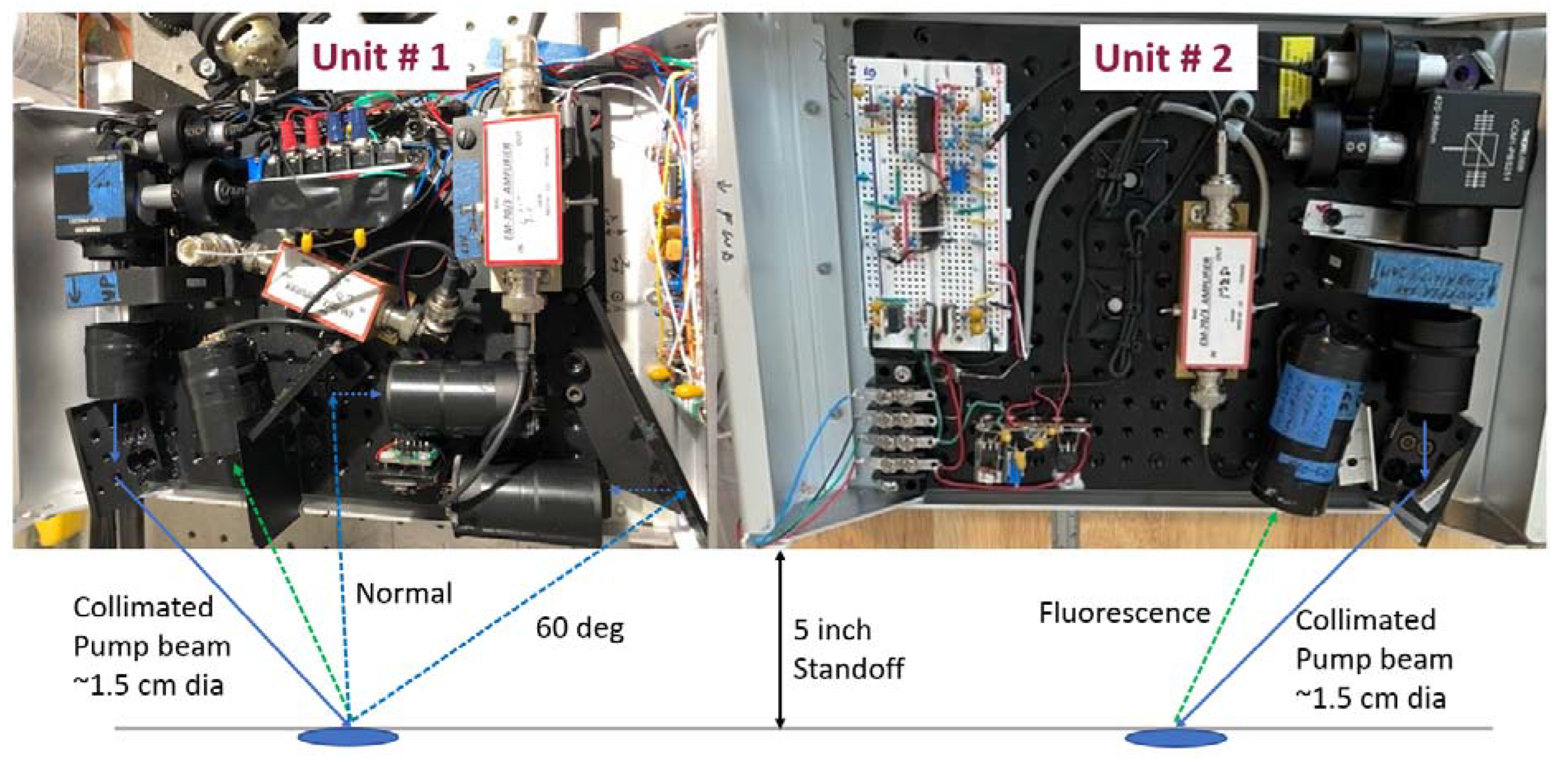
Based on the chemical properties of the grease fluorescence, an optical sensing system was developed by RTL to measure a grease’s emitted fluorescent intensity on the flange face, thereby determining its presence on the rail. This system comprises two 405 nm lasers, a fluorescence band-pass filter, and a fluorescence optical detector. The two linearly polarized lasers are arranged in a cross-polarized setup to minimize laser optical speckle. Since the lasers operate independently, their wavelengths are nearly identical for detecting rail grease fluorescence. Slight wavelength differences between the two lasers are used to eliminate effects like speckle modulation when they are used to illuminate the same grease volume. The lasers generate an incident coherent beam onto the flange face of the rail to create an illumination volume in the grease. The volume is bounded by the thickness of the grease and the laser beam’s illumination spot on the rail surface. An optical detector, oriented near 60 degrees to the longitudinal rail surface, measures the grease’s emitted fluorescence intensity. This angular configuration was determined to provide the best signal-to-noise ratio (SNR) through a series of tests that evaluated various beam configurations. The detailed working mechanism of the RTL system can be found in [
13].
Two lubricity detection devices, referred to as “Unit 1” and “Unit 2”, were fabricated to monitor the lubrication conditions on the left and right rails, as shown in
Figure 2. Both units are equipped with identical laser emitters and filters. Both devices are aligned and angled toward the rail surface using identical geometric configurations, with the sole distinction that one unit mirrors the other one in down-track beam orientation. This setup ensures that each rail is evaluated at an identical interception angle relative to the cart’s movement along the rail. The two units were initially mounted to a controlled robotic cart, shown in
Figure 3, which will be detailed later.
3. Rail-Cart-Mounted RTL System
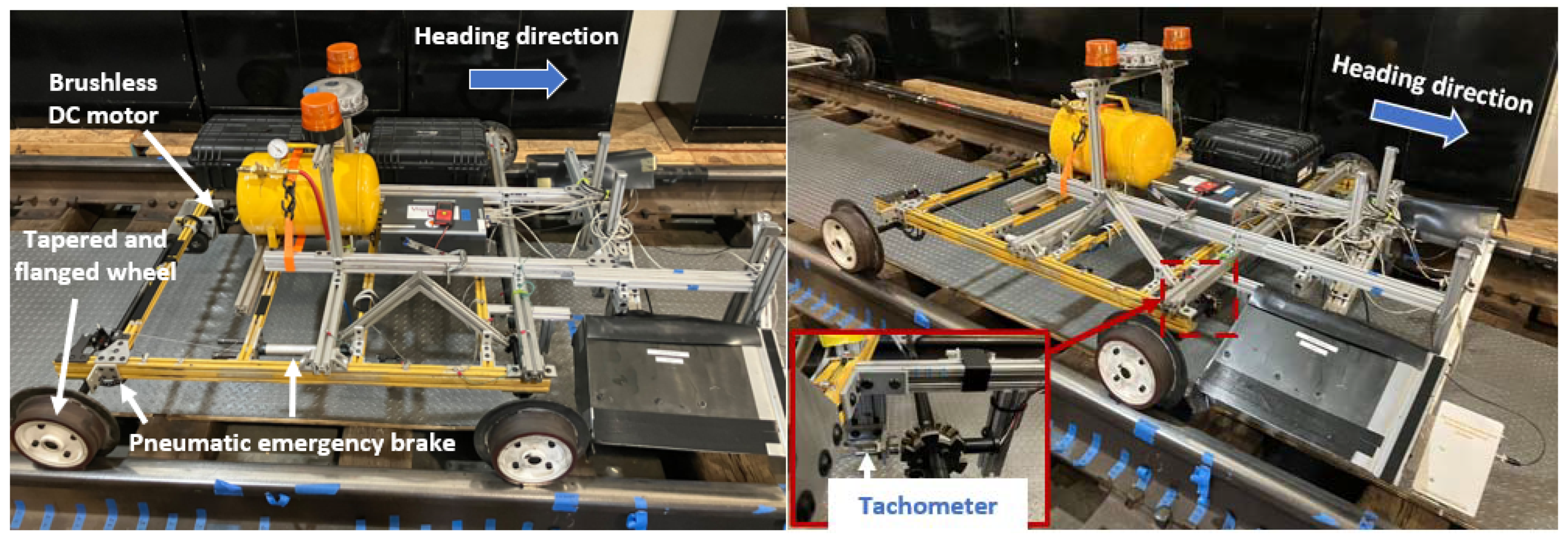
The remotely controlled rail cart used for testing includes an electric propulsion and braking system to ensure safe operation on active service tracks [
22]. The cart can operate up to 10 mph (16 km/h.). A tachometer is mounted on the front axle to measure and record wheel rotations, providing data to calculate the cart’s speed and distance traveled. The tachometer data are recorded at a frequency of 125 Hz, providing accurate measurements of the distance traveled. As illustrated in
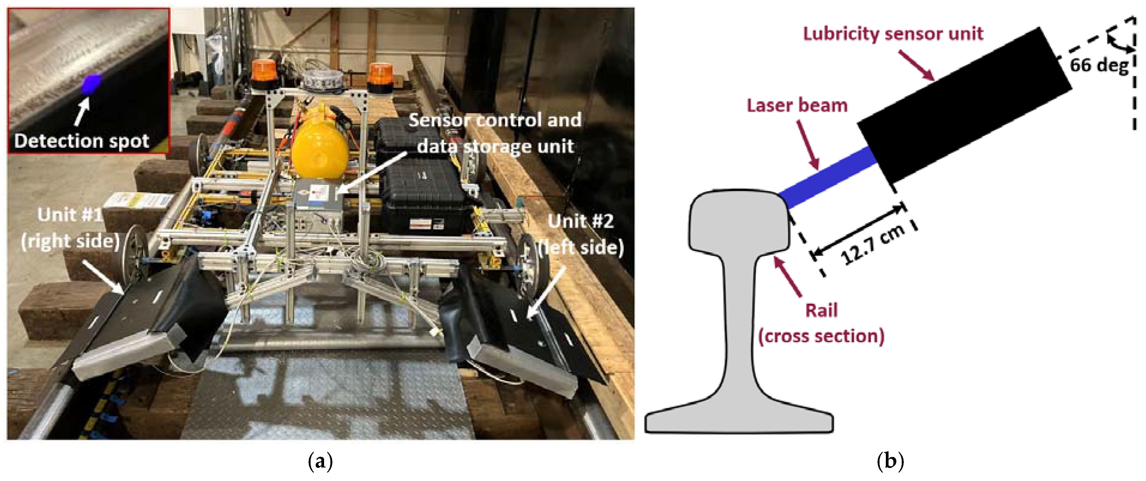
Figure 3a, the two units are positioned ahead of the cart’s leading wheels, with Unit 1 on the right and Unit 2 on the left, allowing measurements before the cart’s wheels and flanges disturb the grease. As shown in
Figure 3b, each unit is positioned at a 66-degree angle relative to the vertical axis at a standoff distance of 5 inches (12.7 cm). This configuration ensures that the laser beam targets specific spots on the side of the railhead, where flange-face grease is typically applied, as shown in
Figure 3a.
4. Effect of Thickness on Fluorescence Properties
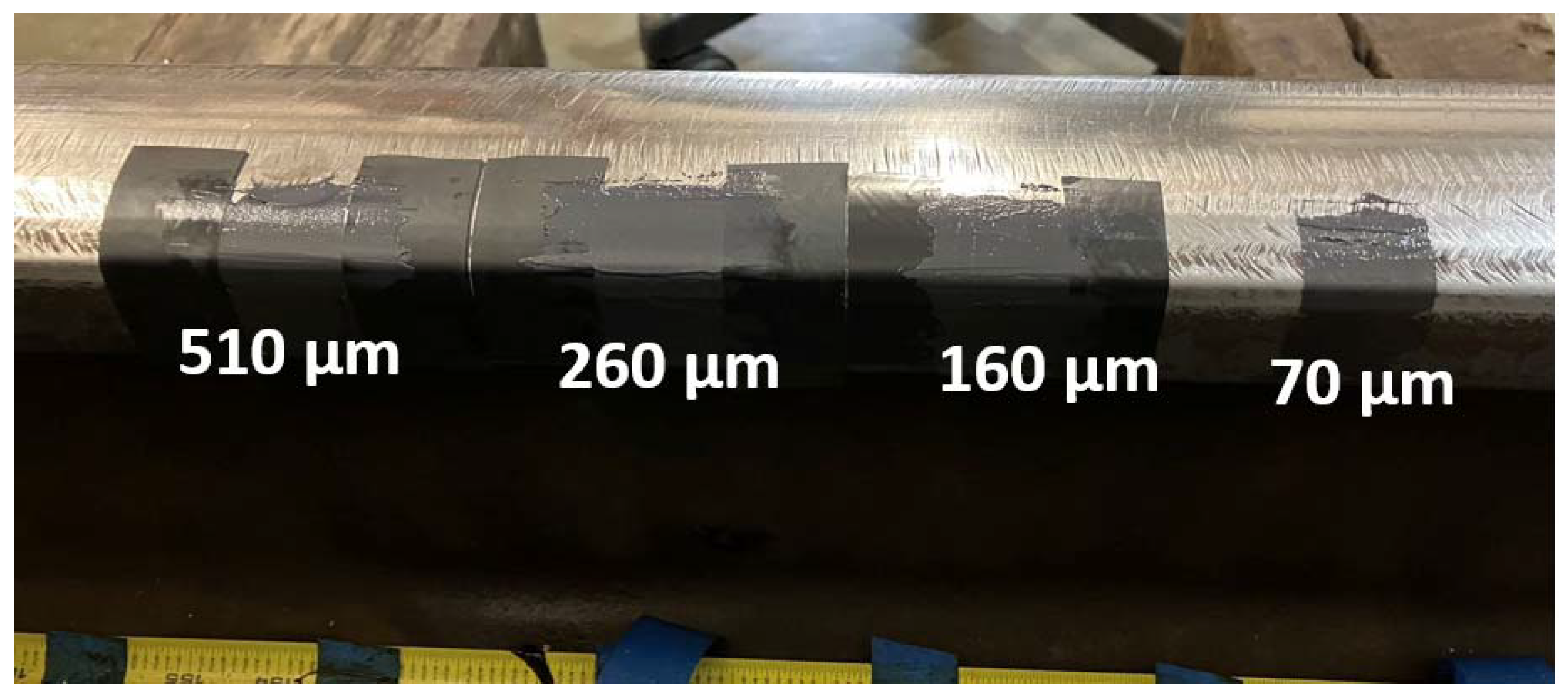
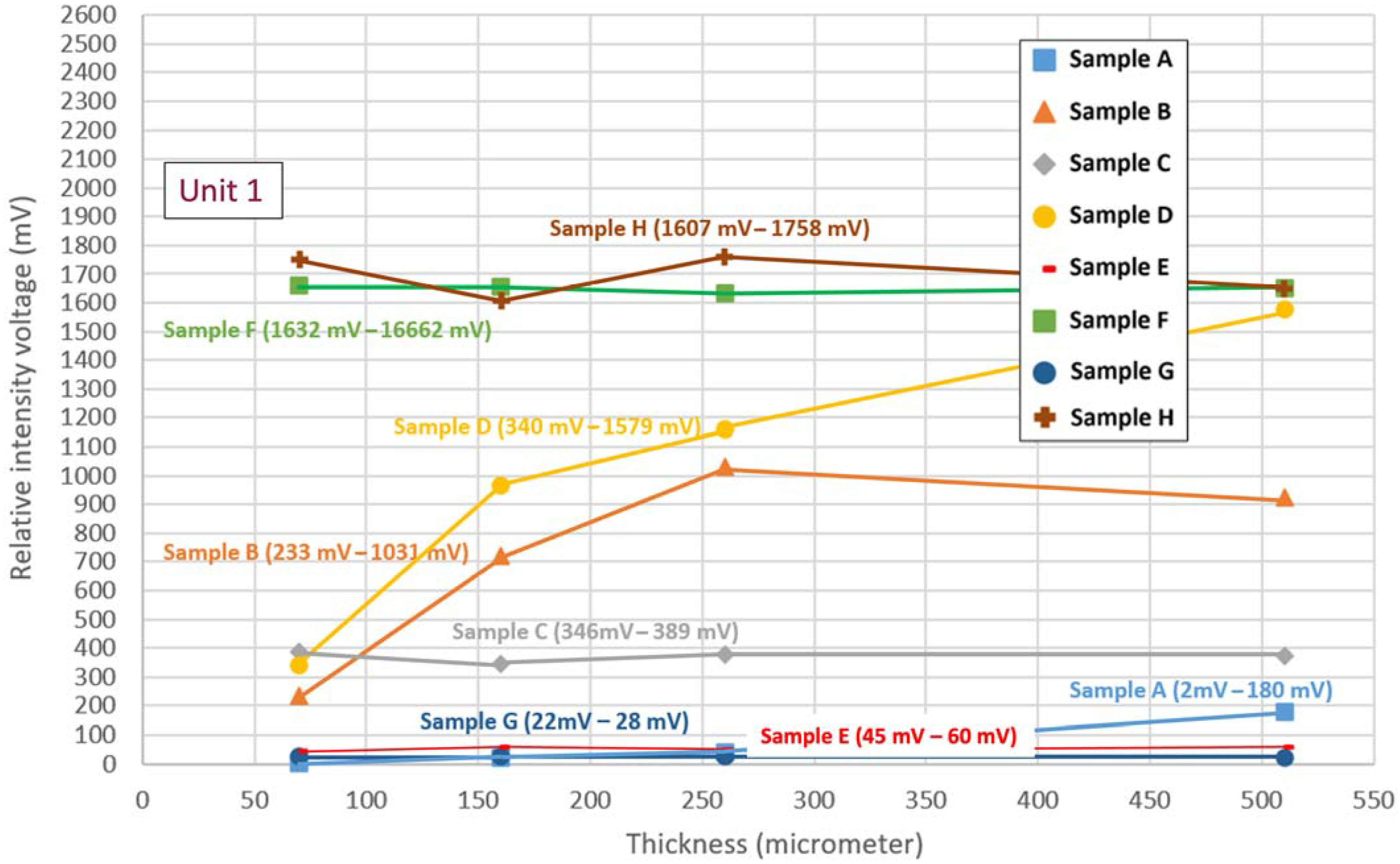
Laboratory tests were performed on a 40 ft track panel at the RTL facility to study the change in fluorescence intensity with grease thickness. Eight grease samples (Sample A to Sample H) were evenly distributed on the flange corner and flange face at varying thicknesses, ranging from 70 to 510 µm.
Figure 4 shows one of the eight samples (Sample A) applied on the inner rail head corner. As the rail cart moves forward on the track, the two units measure the fluorescence intensity emitted by the grease, which is directly related to the presence and thickness of the grease, as mentioned earlier.
Figure 5 displays the results for Unit 1 showing the variation in fluorescence at different thicknesses for the eight different grease samples applied. The samples were acquired from the major manufacturers that supply grease to the U.S. railroads. Since the results for Unit 2 were similar to those of Unit 1, only the results for Unit 1 are presented for brevity. The results indicate a nonlinear correlation between the sensor output voltage and grease thickness for thicknesses below the extinction depth. The extinction depth marks the depth at which the light passing through the grease drops to less than 10% of its original intensity at the surface. This depth varies for each grease sample and depends on the specific composition and materials used in the grease. The extinction depths for the tested samples were between 25 µm and 150 µm. When the grease thickness exceeds the extinction depth, the fluorescence emission intensity remains constant, irrespective of the thickness. This observation applies to all tested greases, except for Samples A and D, which have extinction depths beyond the considered thickness range. Therefore, its intensity voltage always increases with thickness within the considered range of rail application. The grease samples with higher relative intensity voltage even at lower thicknesses, like Sample F and Sample H, are more detectable.
5. Effect of Lateral Movement on Fluorescence Signals
The LFOM sensors shown in
Figure 2 were principally designed to operate at a fixed standoff distance from the rail surface of 5 inches to maximize the strength of the fluorescence signal and reduce interference from scattered laser light. However, this optical arrangement can cause the fluorescent signal to vary due to unwanted variances in the sensor-to-rail standoff distance. The variance is not a problem for mounting on Hyrail vehicles, but the magnitude of the lateral variance in the RTL robotic cart requires compensation of the fluorescent signal in order to accurately assess the thickness of the grease (microns) in the presence of the much larger cart lateral dynamics (inches). When the cart goes around a curve, the centrifugal forces push it outward, pushing the wheel flange toward the side of the railhead. This lateral movement allowed by the running “looseness” in the RTL cartwheel flange/gage separation slightly shifts the intercept position of the laser detection spot on the rail, as illustrated in
Figure 6, which impacts the intensity calibration of the fluorescent measurements and, in turn, affects any assessment of grease thickness.
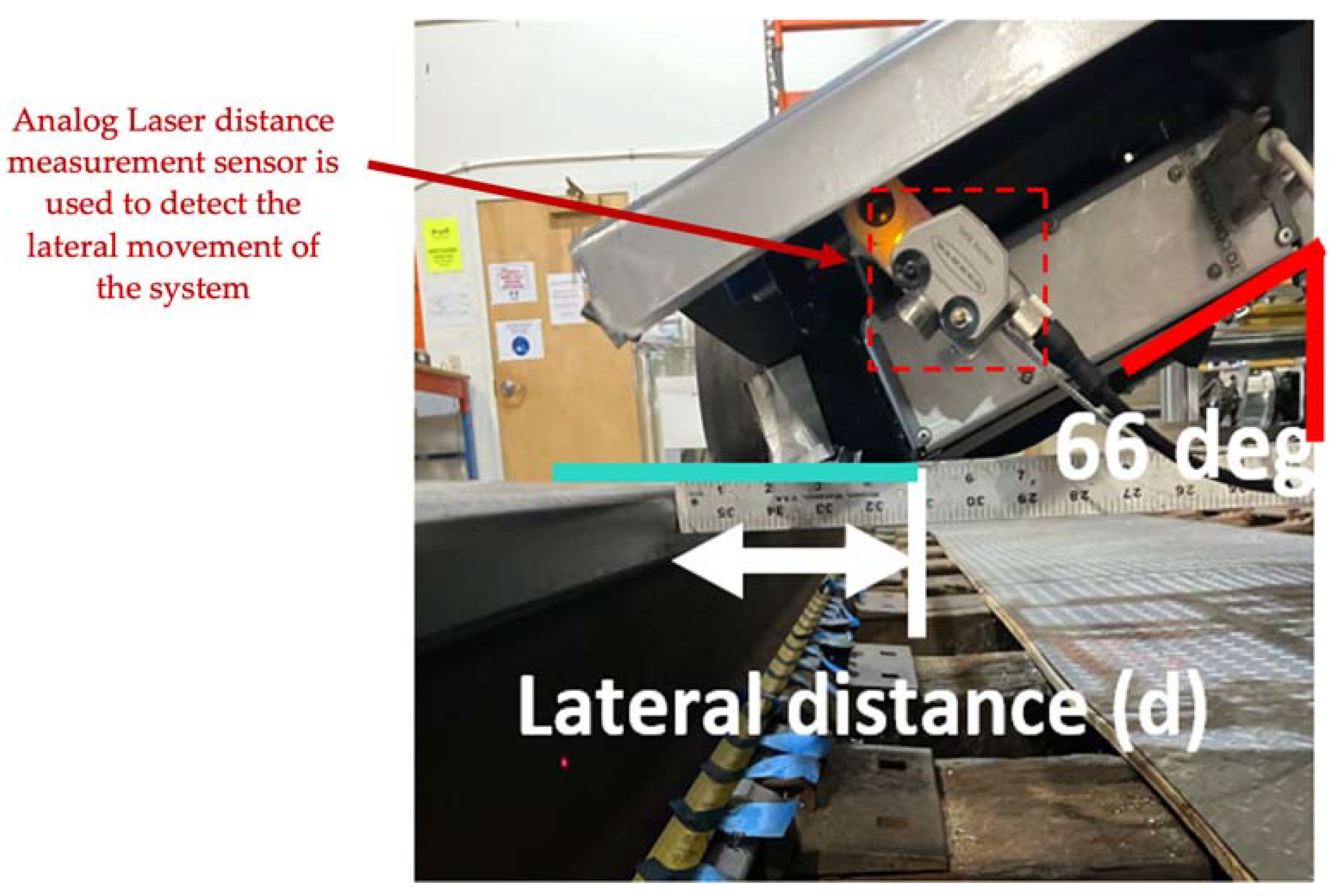
To support compensation of this effect, a Q4X300, 25–300 mm Analog Laser
® distance measurement sensor manufactured by Banner Engineering Inc. in Aberdeen and Huron, South Dakota, USA, is used to detect the lateral standoff distance to the railhead as a proxy for the lateral movement of the cart, as shown in
Figure 7. Calibrations were conducted in the lab to evaluate the effect of cart movement on the LiDAR measurements. Each grease sample was again applied to the rail with an identical thickness of 510 µm, and measurements were made for varying lateral displacement. The calibration results were subsequently used to adjust laboratory and field measurements appropriately from the mounted RTL sensors.
The cart was initially positioned with the right wheel flange in contact with the rail. It was then gradually shifted laterally to the left until the left wheel flange contacts the rail. As the lateral distance (d) increases, the standoff between the laser and the rail increases, and the laser beam spreads, resulting in a larger illumination spot. The beam’s spread reduces the beam’s intensity per unit area, leading to lower magnitudes in fluorescence measurements. Conversely, a shorter standoff distance focuses the beam on a smaller spot, increasing its intensity and generating a stronger fluorescence signal. The readings recorded for Unit 1, as shown in
Figure 8, demonstrate that the fluorescence intensity decreases by as much as 13% as the lateral distance, ‘d’, in
Figure 7 increases.
A calibration curve was fitted to the known data points to obtain ‘d’ from the Analog Laser distance measurement sensor, which included the Analog Laser distance measurements vs. the corresponding actual lateral distance. The calibration curve is shown in
Figure 9, which is used to reflect the effect of laser lateral movement caused by the cart movement in the fluorescence measurements. In knowing the lateral displacement of the LFOM sensors relative to the rail and the variance of the LFOM signal with that displacement, we should, in principle, be able to sufficiently compensate the LFOM sensor fluorescent signal to allow the accurate assessment of grease thickness from the compensated fluorescent signal intensity. However, the accuracy achieved is highly model-dependent. In the next section, we describe a compensation model that is machine learning-dependent.
6. Machine Learning-Based Thickness Prediction Model
Without properly compensating for the platform movement, one cannot use the LFOM measurements to reach an accurate conclusion on the lubricity condition of the inner rail head corner using this particular robotic cart. Traditional correlation-based compensation methods, such as polynomial regression, curve fitting, and rule-based thresholding [
23,
24], often rely on predefined mathematical relationships to model the impact of lateral displacement (‘d’) and laser measurements on grease thickness. Such methods follow a fixed mathematical pattern to link the variables that work well in controlled settings but often fail in field conditions with far more variation. For example, polynomial regression assumes that a smooth mathematical curve can adequately describe the relationship between intensity voltage and lateral displacement. In practice, however, this relationship is affected by additional factors like sensor noise, track irregularities, environmental lighting, and changes in grease composition.
To improve on such a simple approach, machine learning methods were developed for improving the estimation accuracy. The ML models mainly account for the measurement errors caused by cart or platform movements. Machine learning methods provide a more flexible and adaptive approach by learning directly from data rather than relying on rigid assumptions using a limited parameter set. Instead of manually defining the correction function, ML models can identify complex, nonlinear dependencies between the fluorescent intensity signal, displacement, and grease thickness by analyzing the experimental data. This methodology for compensating the lateral motion effects on fluorescent signal intensity described in the preceding section was pursued to assess field test data.
A custom dataset was prepared by performing a series of laboratory tests in controlled conditions. The details of these lab tests, including the experimental setup and procedure, will be discussed in the next subsection. This lab data was then used to train an ML model.
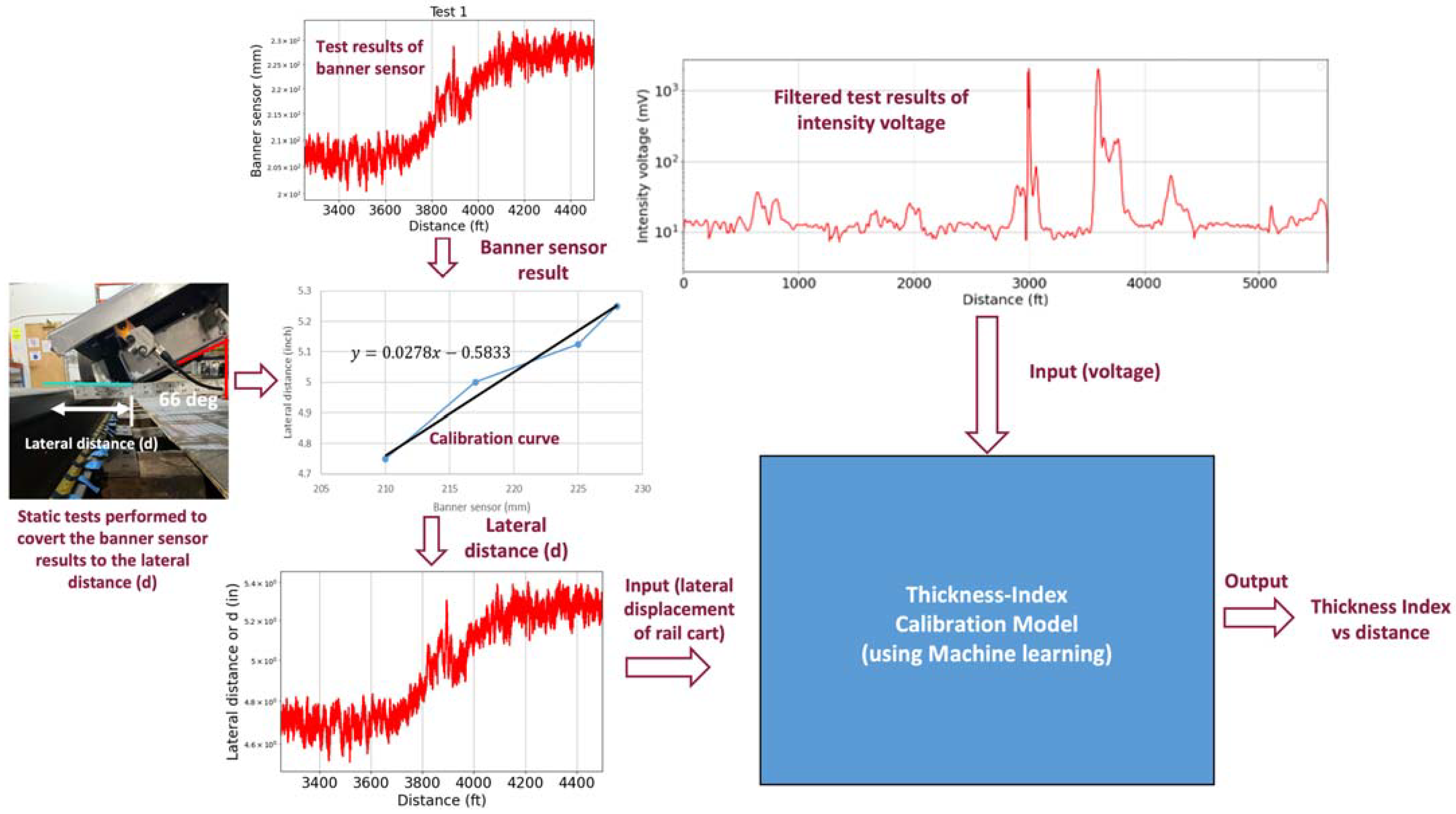
Figure 10 illustrates the framework of the proposed methodology used for the thickness prediction of the grease. The distance LiDAR sensor records the lateral movement of the cart that is plotted against the distance traveled by the cart. Since the measurements do not reflect the absolute value of ’d’, a series of static tests were performed to relate the sensor’s output with actual distances. These values act as one of the two inputs to an ML calibration model. The fluorescence intensity measurements recorded by the RTL system are post-processed and filtered to remove any noise from uncorrelated disturbances. This filtered data acts as the second input to the model. The model then establishes the relationships between the two inputs and predicts the thickness index of flange grease.
6.1. Dataset Preparation
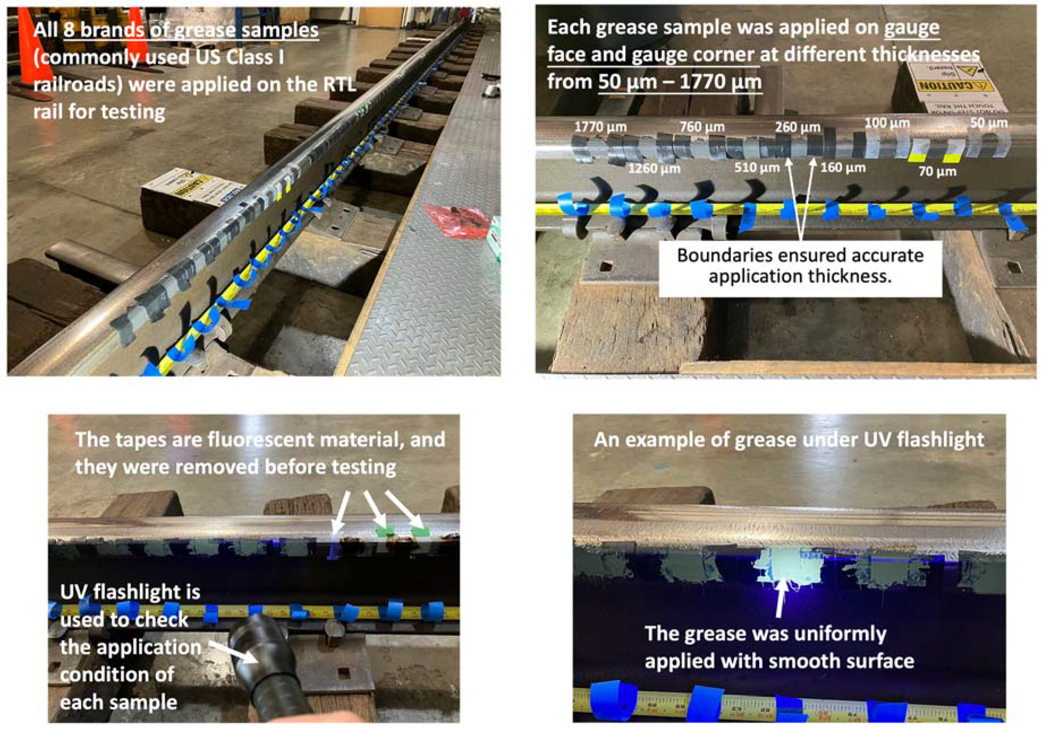
The custom dataset used to train the machine learning model was prepared by performing tests on a 40 ft track panel in the RTL laboratories. Nine grease samples with thicknesses of 50, 70, 100, 160, 260, 510, 760, 1260, and 1770 µm were applied to the flange face of the rail, as shown in
Figure 11. To ensure consistency in grease application, we applied each grease sample between adhesive strips with calibrated thickness.
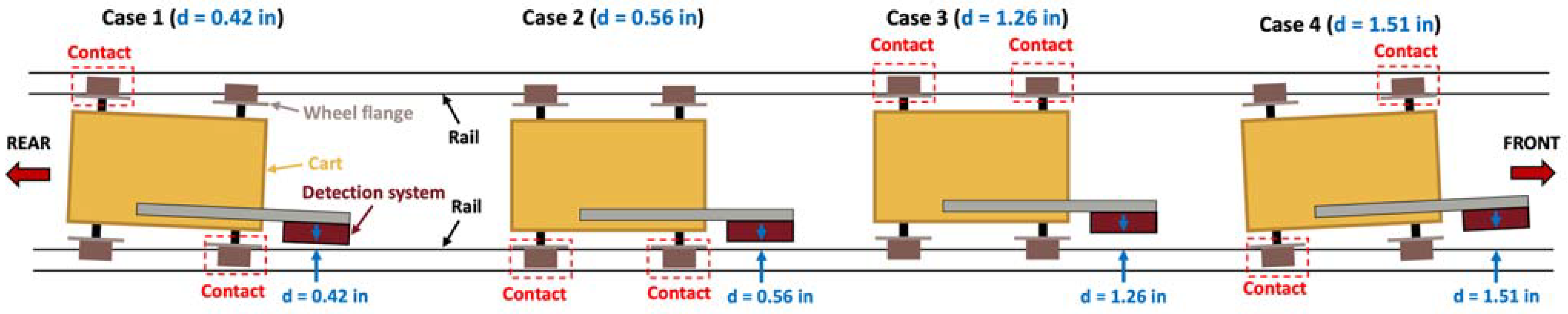
For each thickness, the intensity and displacement (‘d’) voltage measurements from the cart-mounted sensors were made at different lateral positions of the rail cart.
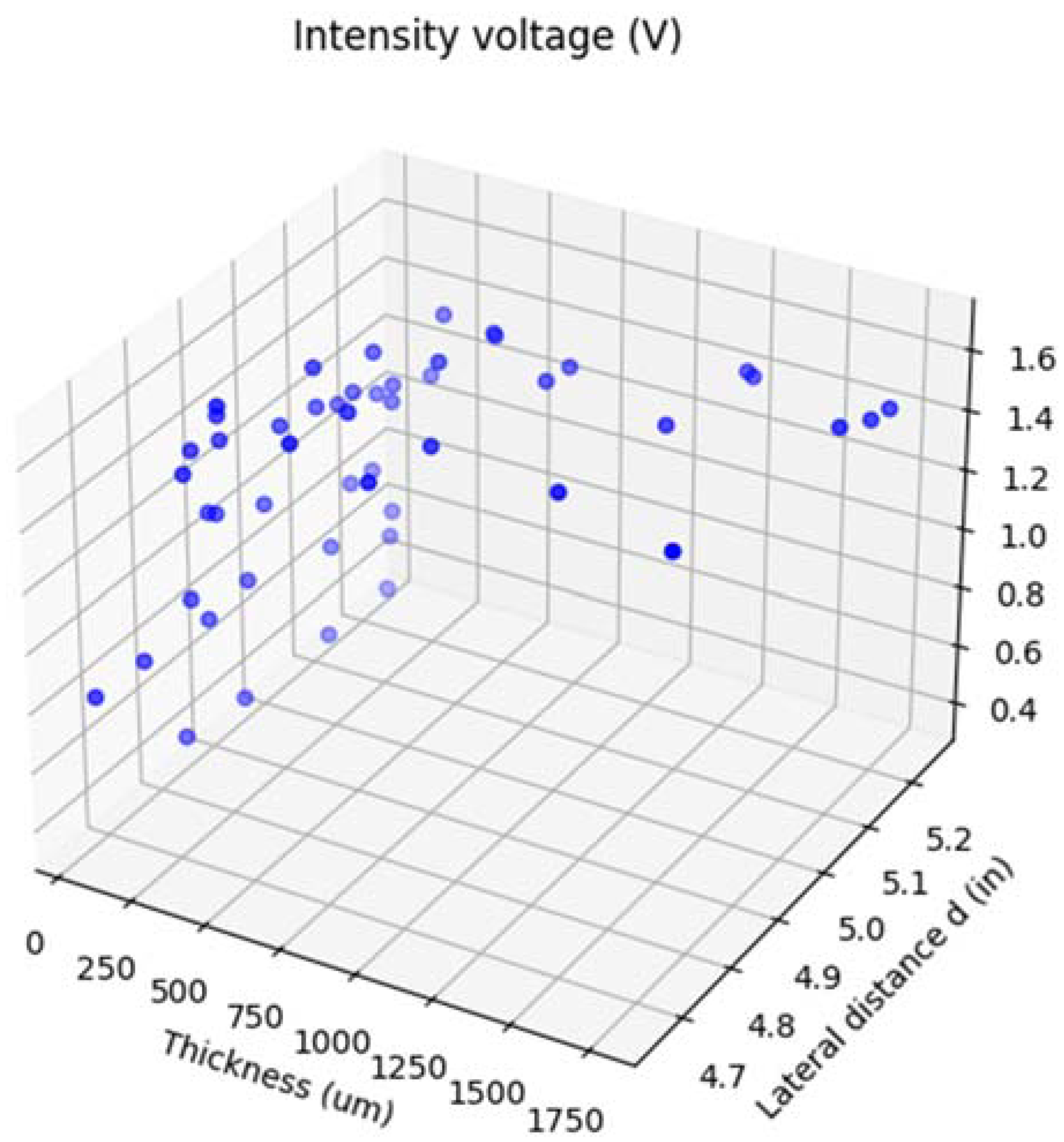
Figure 12 shows plane-view schematics of the rail cart for four cases of the different lateral positions for which the sensor measurements were recorded. A dataset containing 50 data points was assembled from the combination of different thicknesses and values of ‘d’, as shown in
Figure 13. This dataset was then preprocessed as described below before training the model.
6.2. Data Preprocessing
Before training the model, the raw data must be preprocessed to reduce any known artifacts and ensure that the data is in a suitable format to train the model accurately. This step plays a crucial role in reducing any noise or biases present and will further optimize the performance of the model. The dataset was divided into three classes based on the thickness of the grease:
Unlubricated: (thickness index = 0);
Class 0: less than 85 µm (thickness index = 1);
Class 1: 85–385 µm (thickness index = 2);
Class 2: more than 385 µm (thickness index = 3).
The raw intensity voltage signal collected from the RTL sensing system contains a small electronic offset associated with an unlubricated, cleaned section of the test rail, where no grease is present. This offset needs to be removed to represent the actual grease signal better so that the data associated with the unlubricated section would be at zero. After offset removal, the input features for this dataset, lateral displacement (‘d’) and the fluorescent intensity voltage (V), were further normalized to values between 0 and 1 to ensure that they were on the same numerical scale, as shown in
Table 1, a section of the dataset with normalized input features for different thicknesses. In machine learning, a feature refers to an input variable the model uses to learn patterns and make predictions. Mathematically, features are equivalent to variables or parameters, representing measurable properties that influence the model’s performance. Normalization prevents the features with larger dynamic ranges from dominating the model training process, thus ensuring that all features are prioritized proportionately.
The data was split into three subsets to facilitate model training and evaluation; 70% of the data was used for training, 20% for testing and evaluating the model’s performance on unseen data, and 10% for assessing the model’s predictive accuracy. The model’s training was determined to be complete when the model’s predictive quality reached the goal of 90% or better. Data splitting is performed to evaluate the model’s generalizability and prevent overfitting. The resulting “preprocessed” data was then used to train the machine learning model and classify the data into defined thickness indices.
6.3. Machine Learning Model Selection
Classification is a supervised machine learning (ML) technique that trains a model to categorize the input data into predefined classes. With the help of prelabeled training data, the model learns to identify the patterns or features that differentiate the classes and uses this knowledge to predict the class of new, unseen data. For this study, various classifiers like Decision Trees, Support Vector Classifier (SVC), Random Forests, Logistic Regression, and Neural Networks were explored and compared to predict the thickness index of the grease. Each classifier offers its own unique strengths in analyzing the data and the different types of complexities, making it essential to explore the individual characteristics and performance in predicting the thickness index for this application.
Decision Trees is a supervised learning algorithm often used for regression and classification of data. This algorithm is used to represent the data in the form of a tree-like structure where the branches represent the values of the features (input variables) which are recursively created until a decision is reached. This algorithm is mainly known for its high interpretability and simplicity [
25]. Random Forest is an ensemble learning algorithm used for classification and regression consisting of multiple Decision Trees. The decision made by Random Forest is based on the collective decision made by the number of Decision Trees [
17,
26]. Logistic Regression is a statistical model commonly used for classifying binary data with only two outputs (e.g., true/false or 0/1). This algorithm uses a sigmoid function to fit the data by mapping the input to 0 and 1 [
26]. Neural Networks are a subset of machine learning models which consist of interconnected layers of nodes. Each layer of nodes has an activation function that processes the input and passes the output to the subsequent layers. They are mainly used to classify complex and high-dimensional data. SVC is a specialized variant of Support Vector Machine (SVM) tailored for classification problems. After evaluating the performance of each model, the Support Vector Classifier (SVC) was chosen as the most optimal model for this application.
6.3.1. Support Vector Classifier (SVC)
The SVC algorithm operates by identifying a “hyperplane” that optimally separates the data into distinct classes with the maximum margin while minimizing classification errors. The mathematical formulation of SVC is centered around solving the following optimization problem [
27]:
subject to
where
w represents the weights associated with the features;
b is a bias term;
C is a regularization parameter;
εi are the slack variables allowing for misclassification;
yi are the class labels (TI = 0, 1, 2, 3);
xi are the feature vectors (‘d’ and ‘V’).
Since our dataset is not linearly separable, SVM maps input features into a higher-dimensional space using a kernel function [
28]
transforming the optimization problem into
where
αi are Lagrange multipliers obtained by solving this optimization;
K(xi,xj) is the kernel function which maps input data into a higher-dimensional space.
We used a Radial Basis Function (RBF) kernel, which is formulated as
where
controls the influence of each training sample
6.3.2. Hyperparameter Tuning
The generated dataset was used to train the Support Vector Classifier. The performance of an SVC model is highly dependent on hyperparameters, particularly C (regularization parameter) and gamma (
). ‘C’ controls the trade-off between margin maximization and classification error, while ‘
’ determines the influence of individual training samples on the decision boundary. Hyperparameter tuning is essential to ensure that the model achieves the best generalization ability while avoiding underfitting or overfitting. To optimize model performance, GridSearchCV, an exhaustive search-based hyperparameter tuning technique, was employed [
29]. GridSearchCV systematically evaluates all possible combinations of specified hyperparameter values using cross-validation, a technique that partitions the dataset into multiple training and validation subsets to assess model performance on unseen data. By iterating over different hyperparameter settings and averaging results across these subsets, cross-validation helps prevent overfitting to a specific portion of the data. The model is trained multiple times with different hyperparameter configurations, and the combination that yields the highest cross-validation accuracy is selected as the optimal set of parameters. In this study, GridSearchCV explored the hyperparameter space for C = {0.01, 0.1, 1, 10} and γ = {‘scale’, 0.0001, 0.001, 0.01, 0.1} for a cross-validation (CV) value of 5. The best parameters were found to be C = 1 and γ = ‘scale’. In SVC, the ‘scale’ option for γ is an automatic setting that adjusts γ based on the input features. When γ = ‘scale’, it is computed as [
30]
where
is the number of features and
is the variance of the dataset. This setting ensures that
is inversely proportional to the variance of the data, making it adaptive to the dataset’s spread instead of requiring a manually chosen value.
6.3.3. Convergence Curves
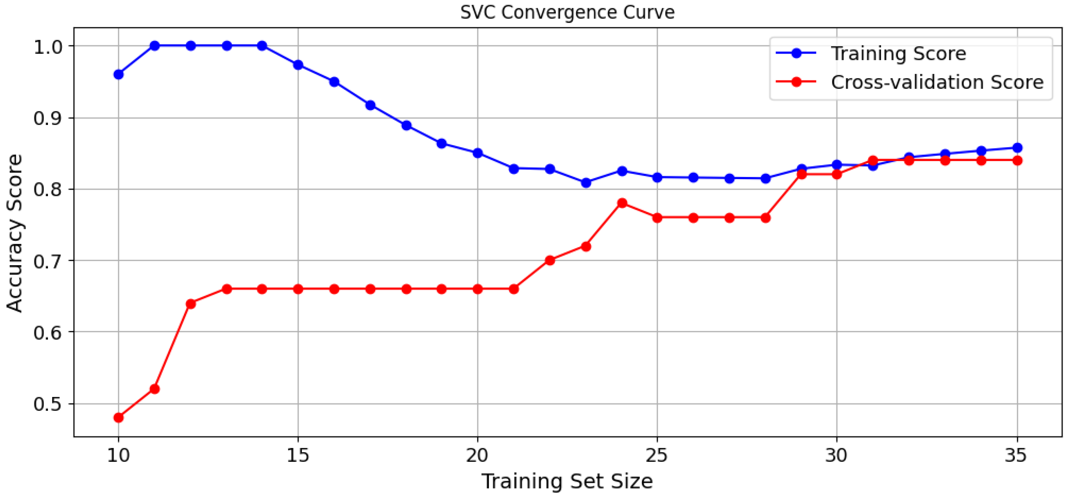
To further assess the model’s performance, we plotted the convergence curve illustrating the training scores and validation scores across different training sizes, as shown in
Figure 14. The curve provides insights on how the training and cross-validation accuracy evolve as the number of training samples increases. Out of the 50 samples in the dataset, 35 samples (70%) were used for training. The curve shows respective scores for training samples between 10 and 35 because a lower number of samples did not make a significant contribution to the cross-validation scores. The training score (blue curve) starts near 100% when very few samples are available, indicating overfitting to a small dataset. However, as the dataset grows, the training score gradually decreases and stabilizes around 89%, reflecting improved generalization. The cross-validation accuracy (red curve) starts much lower (~50%) due to limited data for generalization but steadily improves as more samples are added, eventually converging near 83–84%. The gap between training and validation accuracy narrows, confirming that the model is not overfitting. This convergence suggests that the selected hyperparameters (C = 1, γ = ‘scale’) effectively balance bias and variance, ensuring stable generalization.
In addition to analyzing the training and cross-validation accuracies, we also examined the loss function to understand the iterative learning process of the SVC algorithm.
Figure 15 shows the loss function curve over 100 iterations performed during the training process. The curve initially shows a steep decline indicating that the model rapidly adjusts its parameters to minimize classification errors. The oscillations observed in the first 20–30 iterations are due to learning rate adjustments, as the model optimizes its decision boundary. After approximately 30 iterations, the loss function curve stabilizes around 0.4, suggesting that the model has converged.
After tuning the model, the training and test accuracies were evaluated to assess the classifier’s performance and generalization. The training accuracy was 86%, and the test accuracy was 80%, indicating that the model generalizes well to unseen data. Since the model performs similarly on both training and testing sets, it is not overfitting and hence shows that the selected parameters provide a good trade-off between model bias and variance in the output and performance.
6.4. Model Validation Through Blind Tests
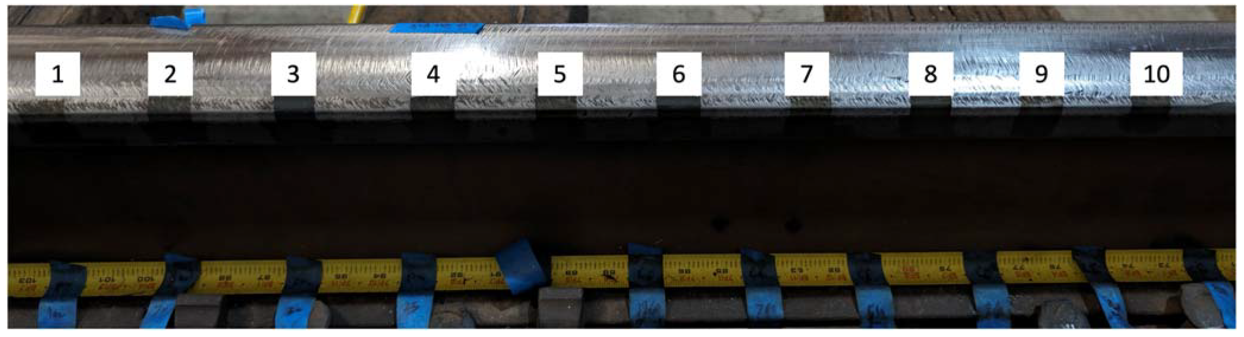
To evaluate the accuracy of the developed machine learning model, we conducted blind tests on the RTL track panel to assess its performance on completely unseen data. For these tests, 10 grease samples with controlled thicknesses were applied to the inner rail head corner, as shown in
Figure 16. The thickness values of each grease sample applied were known to the track engineer, while the Data Scientist was not provided with this information. After the tests were completed, the sensor readings for each sample were collected and provided to the Data Scientist. The ML model was employed to predict the thickness indices. The predicted results were then verified with the known thickness values, by the track engineer, for an unbiased evaluation of the model’s accuracy.
As summarized in
Table 2, only 1 out of the 10 samples was misclassified, resulting in 90% accuracy, successfully validating the effectiveness of the developed model. In the future, we intend to perform more tests to improve the detection accuracy of the model further.
6.5. Model Application: Low-Speed Field Tests and Analysis
The optical sensing system’s ability to detect grease and the machine learning model’s accuracy in predicting thickness under revenue service track conditions were evaluated through low-speed field tests on a curved section of a local Class 1 railroad track.
6.5.1. Test Setup
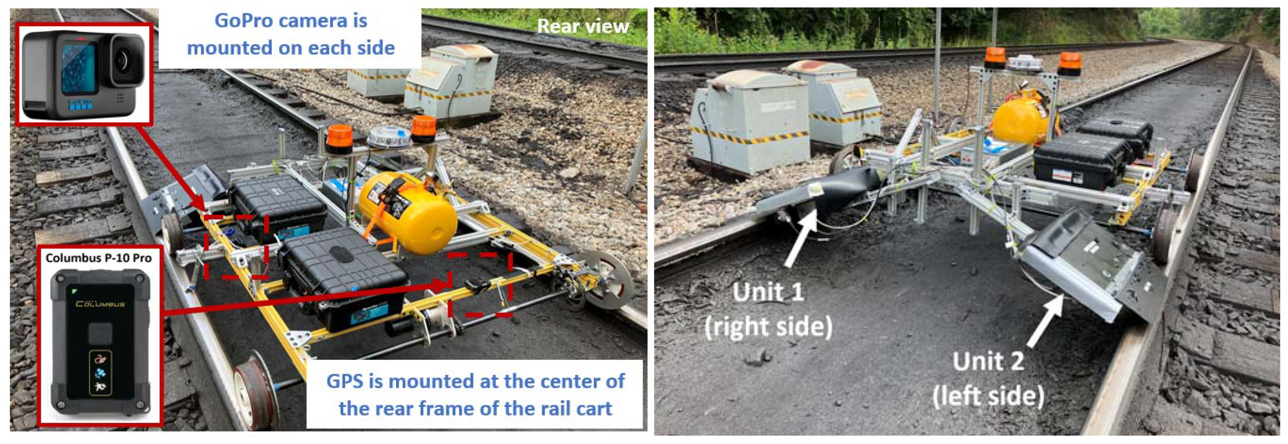
For the low-speed field tests, Unit 1 and Unit 2 were again mounted on the rail cart, one on each side, to simultaneously assess grease conditions on both rails, as shown in
Figure 17. The rail cart, designed for remote control, enabled lubricity detection tests to be conducted at up to 10 mph speeds. For “low-speed” testing, the cart was typically driven at 2 to 5 mph speeds. A Global Navigation Satellite System (GNSS) receiver was mounted on the rear of the cart frame to track the rail cart’s path and speed, as shown
Figure 17. A tachometer installed on the front axle of the cart was used to measure the rotation of the axle to measure the instantaneous vehicle speed and travel distance more precisely than what is available from the GNSS. Cameras by GoPro, Inc. manufactured in San Mateo, CA, USA, were also installed on the cart to visibly record the lubricity conditions of both the left and right rails.
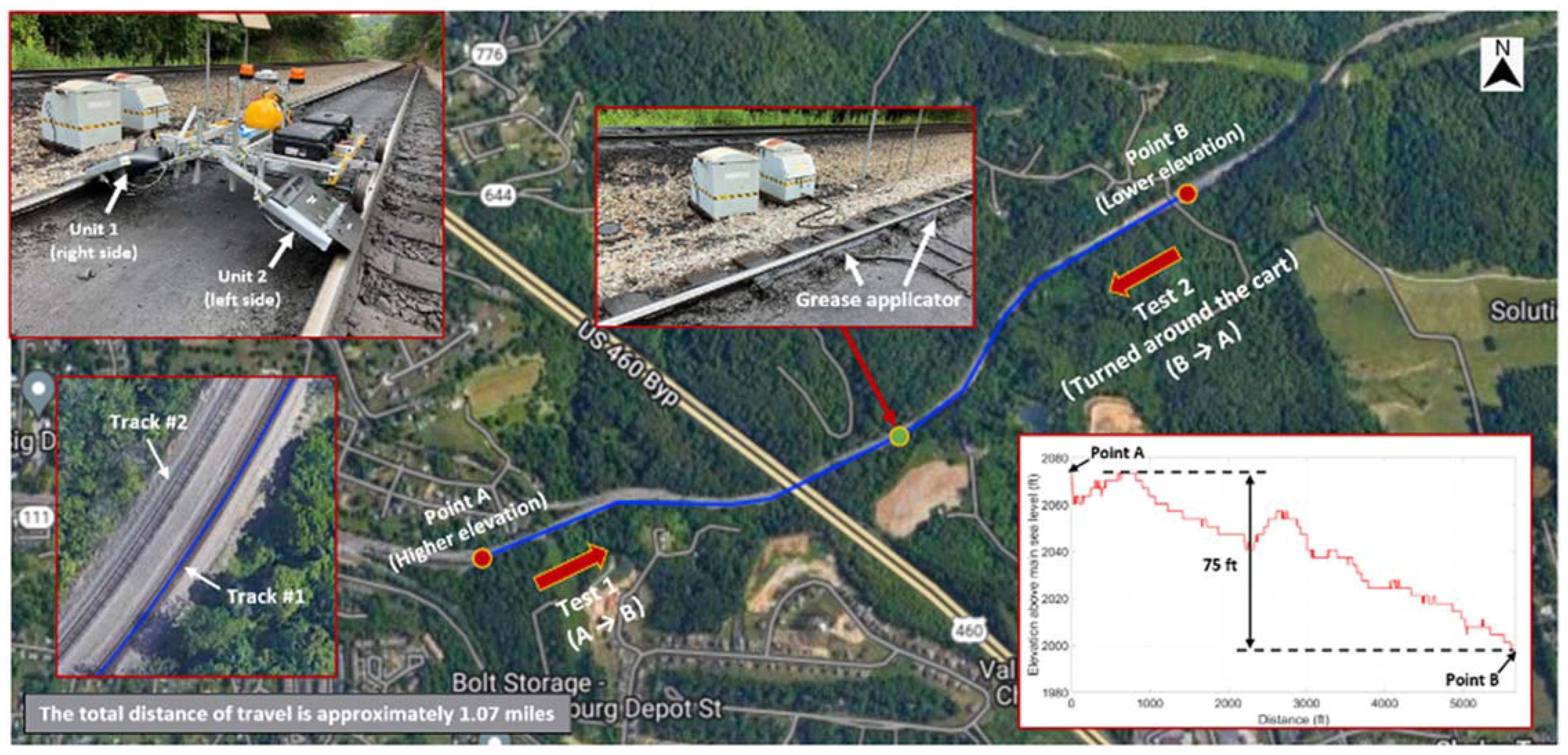
The low-speed field test was conducted on a revenue service track in Christiansburg, VA, with help from one of the Class 1 railroads. The test route, cart setup, and change in elevation are shown in
Figure 18. During the test, the rail cart was initially run from Point A to Point B in
Figure 18, covering a total distance of 1.07 miles and passing through a rail grease applicator, identified by the green dot. The cart was then turned around and operated from Point B to the starting point, Point A.
6.5.2. Field Data Preprocessing
The raw field data collected from the RTL sensing system measurements from the track tests was initially cleaned and processed using our standard analog and digital signal processing, filtering, and scaling techniques.
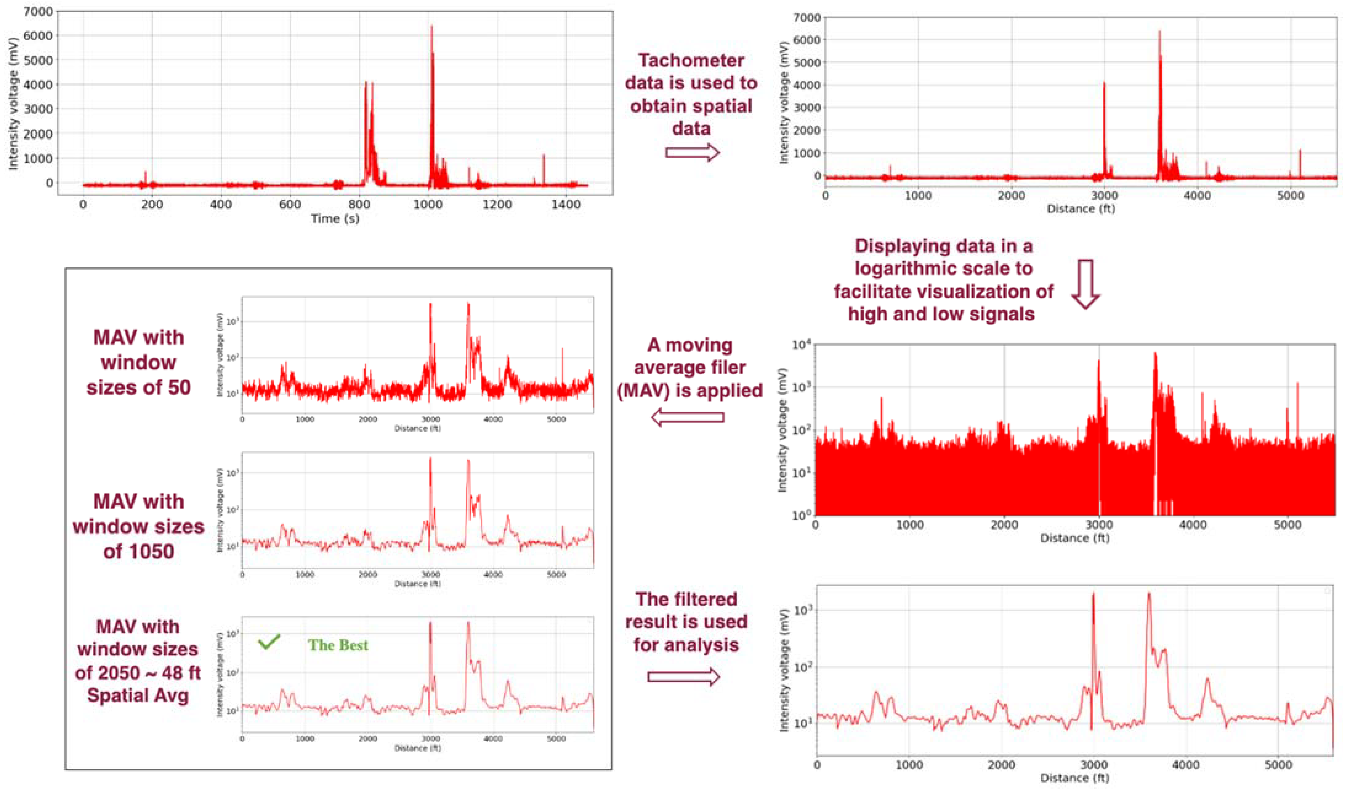
Figure 19 contains a flowchart illustrating the process of analyzing the raw fluorescence intensity measurements collected from the sensing system to assess the spatial lubrication condition of the rail’s flange face.
The tachometer measurements were used to convert the raw data from the time domain to the spatial domain. The data was divided into segments based on individual tachometer pulses that acted as spatial markers. Each 1.868 inch. (3.0145 cm) pulse was used to convert the temporal LiDAR data to spatial measurements that reflect the distance traveled on the track.
The fluorescence intensity varies significantly in amplitude due to the highly uneven grease distribution on the rails. The variation is attributed to the uneven transfer of grease along the track by the wheels passing the point of application (i.e., the applicator). Heavier lubrication yields larger measurement amplitudes, while lighter lubrication yields smaller amplitudes. Given the wide dynamic range in the fluorescent signal, the data is plotted on a semi-log scale in
Figure 19. The original data contains a lot of random noise and fluctuation, even after the averaging process that happens when converting time to displacement. Rail lubrication conditions depend on long-term trends in the data, so it is essential to average the data further to highlight the low-frequency content. A moving average filter was used to filter out high-frequency noise and further smooth the data in the spatial datasets. This type of filter reduces the high-frequency fluctuations by averaging a specified number of data points within a moving window, better revealing underlying trends or patterns in the data. No separate calibration for the vertical movement of the cart is required because the vertical movements due to any objects present on the track or any track irregularities are very sudden. They do not affect the fluorescence readings over the long term. The moving average filter acts as a low-pass filter, effectively filtering out any fluctuations in the data due to these vertical movements.
6.5.3. Down-Track, Spatial Distribution of the Thickness Index for Lubricity Visualization
The developed machine learning model was then used to calculate each point’s thickness index (TI) for both rails from the field data. A color-coded, graphical data visualization format was then developed to display the spatial distribution of the resulting “lubricity” data for use by railroad engineers and maintenance personnel. For brevity,
Figure 20 presents the results obtained from Unit 1 for just one rail. Considering the local direction of track curvature, we found that the spatial distributions of the rail grease on each rail were quite similar. The top plot represents the fluorescent intensity magnitude from the RTL system along the traveled distance, which directly correlates to the grease concentration on the rail. Zero feet in the plot corresponds to the position of the track/rail grease applicator, where an expected spike in fluorescence is observed due to the heavy amount of grease being present at the source. The observed grease distribution before and after the 0 ft position is a result of the grease being carried by train wheels as they pass over the applicator. Since the rail traffic operates in two directions, the grease is distributed in both directions relative to the location of the applicator. Beyond the applicator, spikes in fluorescence, such as those between the 0 ft and 1000 ft mark, occur due to heavy lubrication on curved sections of the track. This lubrication is crucial in reducing wear at the wheel–rail interface, as trains experience strong lateral forces while navigating curves. Based on the LFOM measurements and the Analog Laser distance sensor measurements, the trained ML model predicts the TI of the grease. The bottom graphic in
Figure 20 shows the color-coded TI as a function of distance from the applicator. Heavily lubricated sections with TI = 3 are represented with green color, medium lubrication zones (TI = 2) with yellow, lightly lubricated (TI = 1) with orange, and unlubricated sections (TI = 0) with red color. The chart represents grease thickness across different sections of the track, helping track engineers identify well-lubricated areas and pinpoint sections that require additional lubrication for optimal maintenance. The correlation of the tricolor chart with the RTL system measurements helps assess the model’s performance.
7. Discussions
This paper presents the development of a machine learning model to estimate the TI of flange-face grease using RTL’s optical sensing system. The model demonstrates 90% accuracy in classifying unseen TI data. The current accuracy level, while promising, may still pose challenges for maintenance decision-making, especially in critical rail sections requiring precise lubrication management. One contributing factor to this limitation is the dataset size, as the model was trained using data collected from controlled in-house lab tests with a limited number of data points. Expanding the dataset through extensive field testing under diverse operational conditions can significantly enhance the model’s performance, improving its predictive accuracy and overall robustness for practical deployment.
Additionally, the impact of external operating conditions such as train speed and environmental factors remains an area for further investigation. The field test presented in this paper was conducted at lower speeds of up to 10 mph. Higher speeds of up to 100 mph will have a significant effect on the spatial resolution of the data. Furthermore, extreme cold temperatures or snow accumulation on the rail surface could obstruct the laser from reaching the grease layer, preventing accurate fluorescence readings. Future work will include the assessment of rain on the fluorescence properties of the grease.
Beyond railway lubrication monitoring, the proposed methodology aligns with broader long-term monitoring applications across multiple engineering and industrial sectors. Similar machine learning-driven condition monitoring techniques have been successfully utilized in seismic event detection, where Bayesian fusion helps mitigate faulty data interference and enhances the accuracy of real-time monitoring [
31]. Seismic event detection systems often rely on multiple sensor networks, and Bayesian fusion helps integrate readings from different sources to distinguish genuine seismic activity from noise [
31]. This approach improves sensitivity while reducing false alarms, making it highly effective in automated earthquake early-warning systems.
Additionally, in rotating machinery diagnostics, such as planetary gearboxes, time–frequency representation techniques combined with deep reinforcement learning have improved fault detection and predictive maintenance capabilities. Time–frequency analysis allows for the decomposition of non-stationary vibration signals, enabling precise identification of wear patterns and early-stage mechanical failures [
32,
33]. When coupled with deep reinforcement learning, these methods enable predictive maintenance strategies that adapt dynamically to changing operating conditions, reducing downtime and improving the longevity of industrial equipment. The synergy between sensor-driven monitoring, advanced signal processing, and AI-based decision-making underscores the versatility of the proposed approach in various industrial applications.
8. Conclusions
The results of field testing a laser-based system for measuring flange grease on railroads are presented. The data from low-speed revenue service field tests were used to assess the extent and spread of flange grease past an applicator. A robust, machine learning-based method was introduced for predicting the grease thickness. The measurement system uses 405 nm laser sources, a fluorescence light filter, and a fluorescence optical detector to detect the fluorescence emitted by the grease under laser excitation. Using the fluorescence data, we developed a Support Vector Classifier (SVC) machine learning model to predict the thickness levels of the detected flange grease. This model compensated for the variations in thickness estimations caused by the lateral movement of the robotic rail cart to field the sensors on track. By integrating lateral displacement data and fluorescence intensity measurements, the SVC model was trained to efficiently classify the local thickness of the grease into four thickness indices (TIs), heavy (TI = 3), medium (TI = 2), light (TI = 1) and low/no (TI = 0) lubrication, with an accuracy of 90%. The preparation of the dataset to train the model, using laboratory tests, validation of the model through blind tests, and deployment of the model for low-speed field testing, was discussed in detail. Future work intends to explore scaling this system to higher-speed tests toward achieving routine operational testing by the railroads.
Author Contributions
Methodology, S.M.M., Y.C. and C.H.; experiments, S.M.M. and Y.C.; analysis, S.M.M. and A.R.; writing—original draft preparation, A.R., S.M.M. and M.A.; writing—review and editing, A.R., S.M.M., C.H. and M.A.; supervision, M.A.; project administration, M.A.; funding acquisition, M.A. All authors have read and agreed to the published version of the manuscript.
Funding
This research was funded by the United States Department of Transportation, grant number 693JJ622C000021.
Data Availability Statement
The data presented in this study are available on request from the corresponding author due to privacy.
Conflicts of Interest
The authors declare no conflicts of interest. The funders had no role in the design of the study; in the collection, analyses, or interpretation of data; in the writing of the manuscript; or in the decision to publish the results.
References
- Fröhling, R.; De Koker, J.; Amade, M. Rail Lubrication and Its Impact on the Wheel/Rail System. Proc. Inst. Mech. Eng. Part F J. Rail Rapid Transit 2009, 223, 173–180. [Google Scholar] [CrossRef]
- Waara, P. Lubricant Influence on Flange Wear in Sharp Railroad Curves. Available online: https://www.emerald.com/insight/content/doi/10.1108/00368790110393910/full/html (accessed on 18 January 2025).
- Miyamoto, T.; Suzumura, J.; Nakahashi, J.; Chen, H.; Ban, T. Change in Surface Condition of Turned Wheel and Effectiveness of Lubrication against Flange Climb Derailment. Q. Rep. RTRI 2012, 53, 70–76. [Google Scholar]
- Lewis, S.R.; Lewis, R.; Evans, G.; Buckley-Johnstone, L.E. Assessment of Railway Curve Lubricant Performance Using a Twin-Disc Tester. Wear 2014, 314, 205–212. [Google Scholar] [CrossRef]
- Eadie, D.T.; Oldknow, K.; Santoro, M.; Kwan, G.; Yu, M.; Lu, X. Wayside Gauge Face Lubrication: How Much Do We Really Understand? Proc. Inst. Mech. Eng. F J. Rail Rapid Transit 2013, 227, 245–253. [Google Scholar] [CrossRef]
- Olofsson, U.; Nilsson, R. Surface Cracks and Wear of Rail: A Full-Scale Test on a Commuter Train Track. Proc. Inst. Mech. Eng. Part F J. Rail Rapid Transit 2002, 216, 249–264. [Google Scholar]
- Razak, I.H.A.; Ahmad, M.A.; Puasa, S.W. Tribological and Physiochemical Properties of Greases for Rail Lubrication. Tribol. Online 2019, 14, 293–300. [Google Scholar] [CrossRef]
- Vásquez-Chacón, I.A.; Gallardo-Hernández, E.A.; Moreno-Ríos, M.; Vite-Torres, M. Influence of Surface Roughness and Contact Temperature on the Performance of a Railway Lubricant Grease. Mater. Lett. 2021, 285, 129040. [Google Scholar] [CrossRef]
- Li, S.; Li, J.; Wu, B.; Shi, L.; Zhang, S.; Ding, H.; Wang, W.; Liu, Q. Influence of Lubricating Materials on Wheel-Rail Wear and Rolling Contact Fatigue. Mocaxue Xuebao/Tribol. 2022, 42, 935–944. [Google Scholar] [CrossRef]
- Ebersole, K. Analysis of Wheel Wear and Forecasting of Wheel Life for Transit Rail Operations; University of Delaware: Newark, DE, USA, 2019. [Google Scholar]
- Gyas Uddin, M.; Chattopadhyay, G.; Sroba, P.; Rasul, M.; Howie, A. Wayside Lubricator Placement Model for Heavy Haul Lines in Australia. In Proceedings of the Conference on Railway Engineering, Wellington, New Zealand, 12–14 December 2010. [Google Scholar]
- Kramer, J. Rail Lubrication–a Solid Future? Railw. Track Struct. 1994, 90, 31–33. [Google Scholar]
- Chen, Y.; Mirzaei, S.M.H.; Holton, C.; Ahmadian, M. Development of an Optical Sensing System for the Detection of Lubricity Conditions on the Rail Gage Face. Int. J. Rail Transp. 2024, 13, 103–119. [Google Scholar] [CrossRef]
- Alarcón, G.; Burgelman, N.; Meza, J.; Toro, A.; Li, Z. The Influence of Rail Lubrication on Energy Dissipation in the Wheel/Rail Contact: A Comparison of Simulation Results with Field Measurements. Wear 2015, 330–331, 533–539. [Google Scholar] [CrossRef]
- Plevris, V.; Papazafeiropoulos, G. AI in Structural Health Monitoring for Infrastructure Maintenance and Safety. Infrastructures 2024, 9, 225. [Google Scholar] [CrossRef]
- Chenariyan Nakhaee, M.; Hiemstra, D.; Stoelinga, M.; van Noort, M. The Recent Applications of Machine Learning in Rail Track Maintenance: A Survey. In Proceedings of the Third International Conference, RSSRail 2019, Lille, France, 4–6 June 2019; Lecture Notes in Computer Science (Including Subseries Lecture Notes in Artificial Intelligence and Lecture Notes in Bioinformatics). Springer: Berlin/Heidelberg, Germany, 2019; pp. 91–105. [Google Scholar] [CrossRef]
- Zhou, X.; Lu, P.; Zheng, Z.; Tolliver, D.; Keramati, A. Accident Prediction Accuracy Assessment for Highway-Rail Grade Crossings Using Random Forest Algorithm Compared with Decision Tree. Reliab. Eng. Syst. Saf. 2020, 200, 106931. [Google Scholar] [CrossRef]
- Khare, O.; Gandhi, S.; Rahalkar, A.; Mane, S. YOLOv8-Based Visual Detection of Road Hazards: Potholes, Sewer Covers, and Manholes. In Proceedings of the 2023 IEEE Pune Section International Conference, PuneCon, Pune, India, 14–16 December 2023. [Google Scholar] [CrossRef]
- Rahalkar, A.M.; Khare, O.M.; Patange, A.D. Making Informed Decisions in Cutting Tool Maintenance in Milling: A KNN-Based Model Agnostic Approach. arXiv 2023, arXiv:2310.14629. [Google Scholar]
- Phusakulkajorn, W.; Núñez, A.; Wang, H.; Jamshidi, A.; Zoeteman, A.; Ripke, B.; Dollevoet, R.; De Schutter, B.; Li, Z. Artificial Intelligence in Railway Infrastructure: Current Research, Challenges, and Future Opportunities. Intell. Transp. Infrastruct. 2023, 2, liad016. [Google Scholar] [CrossRef]
- Duran, B.; Eftekhar Azam, S.; Sanayei, M. Leveraging Deep Learning for Robust Structural Damage Detection and Classification: A Transfer Learning Approach via CNN. Infrastructures 2024, 9, 229. [Google Scholar] [CrossRef]
- Mirzaei, S.M.; Radmehr, A.; Holton, C.; Ahmadian, M. In-Motion, Non-Contact Detection of Ties and Ballasts on Railroad Tracks. Appl. Sci. 2024, 14, 8804. [Google Scholar] [CrossRef]
- Gonzalez, R.C.; Woods, R.E. Digital Image Processing; Pearson: London, UK, 2008. [Google Scholar]
- Seber, G.A.F.; Wild, C.J. Nonlinear Regression; Wiley: Hoboken, NJ, USA, 2003. [Google Scholar]
- Rivera-Lopez, R.; Canul-Reich, J.; Mezura-Montes, E.; Cruz-Chávez, M.A. Induction of Decision Trees as Classification Models through Metaheuristics. Swarm Evol. Comput. 2022, 69, 101006. [Google Scholar] [CrossRef]
- Kumar Bhagat, N.; Mishra, A.K.; Singh, R.K.; Sawmliana, C.; Singh, P.K. Application of Logistic Regression CART and Random Forest Techniques in Prediction of Blast-Induced Slope Failure during Reconstruction of Railway Rock-Cut Slopes. Eng. Fail. Anal. 2022, 137, 106230. [Google Scholar] [CrossRef]
- Cortes, C.; Vapnik, V. Support-Vector Networks. Mach. Learn. 1995, 20, 273–297. [Google Scholar] [CrossRef]
- Schölkopf, B.; Smola, A.J. Learning with Kernels: Support Vector Machines, Regularization, Optimization, and Beyond; MIT Press: Cambridge, MA, USA, 2002. [Google Scholar]
- Hastie, T.; Tibshirani, R.; Friedman, J.H. The Elements of Statistical Learning: Data Mining, Inference, and Prediction; Springer: Berlin/Heidelberg, Germany, 2009. [Google Scholar]
- Pedregosa, F.; Varoquaux, G.; Gramfort, A.; Michel, V.; Thirion, B.; Grisel, O.; Blondel, M.; Prettenhofer, P.; Weiss, R.; Dubourg, V.; et al. Scikit-Learn: Machine Learning in Python. J. Mach. Learn. Res. 2011, 12, 2825–2830. [Google Scholar]
- Wang, Y.; Xu, W.; Bao, Y.; He, J.; Zhang, Y. Automated Seismic Event Detection Considering Faulty Data Interference Using Deep Learning and Bayesian Fusion. Comput. -Aided Civ. Infrastruct. Eng. 2024, early view. [Google Scholar] [CrossRef]
- Bai, Y.; Cheng, W.; Wen, W.; Liu, Y. Application of Time-Frequency Analysis in Rotating Machinery Fault Diagnosis. Shock. Vib. 2023, 2023, 9878228. [Google Scholar]
- Ye, L.; Ma, X.; Wen, C. Rotating Machinery Fault Diagnosis Method by Combining Time-Frequency Domain Features and CNN Knowledge Transfer. Sensors 2021, 21, 8168. [Google Scholar] [CrossRef] [PubMed]
Figure 1.
Detailed representation of rail surface geometry with key regions and angular gradients.
Figure 1.
Detailed representation of rail surface geometry with key regions and angular gradients.
Figure 2.
The inner assembly of Unit 1 and Unit 2, with the laser beams illuminating a spot of 1.5 cm diameter on the side of the railhead.
Figure 2.
The inner assembly of Unit 1 and Unit 2, with the laser beams illuminating a spot of 1.5 cm diameter on the side of the railhead.
Figure 3.
(a) RTL system mounted on a remote-controlled rail cart; (b) schematic diagram of sensing unit for detecting the lubrication condition.
Figure 3.
(a) RTL system mounted on a remote-controlled rail cart; (b) schematic diagram of sensing unit for detecting the lubrication condition.
Figure 4.
Sample A grease applied at thicknesses ranging from 70 to 510 µm on the inner rail corner.
Figure 4.
Sample A grease applied at thicknesses ranging from 70 to 510 µm on the inner rail corner.
Figure 5.
Fluorescence intensity values of eight grease samples at varying thicknesses for Unit 1.
Figure 5.
Fluorescence intensity values of eight grease samples at varying thicknesses for Unit 1.
Figure 6.
Locations of Purple spot illuminated due to the laser beam for Unit 1 (right side) and Unit 2 (left side) during lateral cart movement.
Figure 6.
Locations of Purple spot illuminated due to the laser beam for Unit 1 (right side) and Unit 2 (left side) during lateral cart movement.
Figure 7.
Analog Laser distance measurement sensor measuring the cart standoff (lateral distance, d) against the side of the railhead.
Figure 7.
Analog Laser distance measurement sensor measuring the cart standoff (lateral distance, d) against the side of the railhead.
Figure 8.
Decrease in laser intensity vs. time as lateral distance ‘d’ between the sensor and rail increases. Top red plot represents the change in lateral distance (in.) over time (s); Bottom red plot represents change in the intensity voltage (V) over time (s).
Figure 8.
Decrease in laser intensity vs. time as lateral distance ‘d’ between the sensor and rail increases. Top red plot represents the change in lateral distance (in.) over time (s); Bottom red plot represents change in the intensity voltage (V) over time (s).
Figure 9.
Calibration curve (Black line) is used to establish the relationship between Analog Laser distance measurement sensor output and lateral distance, d, based on the connected blue dot measurements.
Figure 9.
Calibration curve (Black line) is used to establish the relationship between Analog Laser distance measurement sensor output and lateral distance, d, based on the connected blue dot measurements.
Figure 10.
Machine learning model framework to predict the thickness index of flange grease; Red plots represent the inputs in the form of lateral displacement of rail cart and filtered fluorescence intensity voltage; Blue dots represent the measured data points used for calibration; Black line represents the calibration curve.
Figure 11.
Grease applied at thicknesses ranging from 50 to 1770 µm to conduct a laboratory test for dataset preparation.
Figure 11.
Grease applied at thicknesses ranging from 50 to 1770 µm to conduct a laboratory test for dataset preparation.
Figure 12.
Plane view of Unit 1 on a rail cart, showing cart movement and changes in ‘d’.
Figure 12.
Plane view of Unit 1 on a rail cart, showing cart movement and changes in ‘d’.
Figure 13.
Three-dimensional representation of the relationship between intensity voltage (V), lateral displacement, d (mm), and grease thickness (um).
Figure 13.
Three-dimensional representation of the relationship between intensity voltage (V), lateral displacement, d (mm), and grease thickness (um).
Figure 14.
Convergence curve for the SVC model across different training sizes showing that the model is not overfitting.
Figure 14.
Convergence curve for the SVC model across different training sizes showing that the model is not overfitting.
Figure 15.
Loss function stabilizes as the number of iterations increases during the training of the SVC algorithm.
Figure 15.
Loss function stabilizes as the number of iterations increases during the training of the SVC algorithm.
Figure 16.
Ten grease samples of different thicknesses were applied on the rail for blind tests.
Figure 16.
Ten grease samples of different thicknesses were applied on the rail for blind tests.
Figure 17.
RTL system mounted on rail cart to conduct low-speed field tests on revenue service tracks.
Figure 17.
RTL system mounted on rail cart to conduct low-speed field tests on revenue service tracks.
Figure 18.
The 1.07-mile revenue service track section used for low-speed tests with a rail cart at 3 to 6 mph. Red arrows (with yellow outline) show the directions for Test 1 (Point A to B) and Test 2 (Point B to A); Bottom right corner graph shows the elevation change as a function of distance travelled during Test 1 (Point A to B); Top left corner red box shows the RTL units mounted on the rail cart; Green dot (Yellow outline) in the center shows the position of Grease applicator.
Figure 19.
Methodology implemented to process the raw fluorescence data collected from the RTL sensing system. Red plots: Top left plot–Intensity voltage data as a function of Time; Top right plot–Spatial data obtained from Tachometer; Central right–Spatial data visualized in logarithmic scale; Central left plots–Plots with different window sizes for Moving Average Filter; Bottom right plot: Filtered intensity voltage data as a function of Distance travelled.
Figure 20.
Unit 1 measurements during the low-speed test, and the corresponding thickness indices predicted by the ML model.
Figure 20.
Unit 1 measurements during the low-speed test, and the corresponding thickness indices predicted by the ML model.
Table 1.
A section of the dataset with normalized input features for different thicknesses.
Table 1.
A section of the dataset with normalized input features for different thicknesses.
| Lateral Distance ‘d’ (in) | Intensity Voltage (V) | Thickness (um) | Labels | Lateral Distance ‘d’ (in) Normalized | Intensity Voltage (V) Normalized |
|---|
| 4.8736 | 1.12580 | 50 | 0 | 0.137393 | 0.127327 |
| 4.8883 | 1.10120 | 50 | 0 | 0.137807 | 0.124545 |
| 4.9794 | 1.00647 | 50 | 0 | 0.140376 | 0.113831 |
| 5.1504 | 0.84036 | 50 | 0 | 0.145196 | 0.095044 |
| 5.1947 | 0.82560 | 50 | 0 | 0.146445 | 0.093375 |
| 4.6496 | 0.83913 | 70 | 0 | 0.131078 | 0.094905 |
| 4.7382 | 0.82806 | 70 | 0 | 0.133576 | 0.093653 |
| 4.8588 | 0.79361 | 70 | 0 | 0.136976 | 0.089757 |
| 5.2181 | 0.56476 | 70 | 0 | 0.147105 | 0.063874 |
| 4.8182 | 1.42360 | 100 | 1 | 0.135831 | 0.161008 |
| 4.8711 | 1.38540 | 100 | 1 | 0.137323 | 0.156688 |
Table 2.
Blind test results.
Table 2.
Blind test results.
| Sample Number | Actual Thickness | Actual Index | Predicted Index |
|---|
| 1 | 152 | 1 | 1 |
| 2 | 50 | 0 | 0 |
| 3 | 304 | 1 | 1 |
| 4 | 70 | 0 | 0 |
| 5 | 504 | 2 | 2 |
| 6 | 152 | 1 | 1 |
| 7 | 252 | 1 | 2 |
| 8 | 504 | 2 | 2 |
| 9 | 152 | 1 | 1 |
| 10 | 70 | 0 | 0 |
| Disclaimer/Publisher’s Note: The statements, opinions and data contained in all publications are solely those of the individual author(s) and contributor(s) and not of MDPI and/or the editor(s). MDPI and/or the editor(s) disclaim responsibility for any injury to people or property resulting from any ideas, methods, instructions or products referred to in the content. |
© 2025 by the authors. Licensee MDPI, Basel, Switzerland. This article is an open access article distributed under the terms and conditions of the Creative Commons Attribution (CC BY) license (https://creativecommons.org/licenses/by/4.0/).


