Article

A Numerical Simulation Study on Vertical Vibration Response for Rail Squat Detection with a Train in Regular Traffic

Department of Civil and Environmental Engineering, NTNU-Norwegian University of Science and Technology, 7034 Trondheim, Norway
*
Author to whom correspondence should be addressed.
Infrastructures 2025, 10(11), 313; https://doi.org/10.3390/infrastructures10110313
Submission received: 3 October 2025 / Revised: 9 November 2025 / Accepted: 17 November 2025 / Published: 19 November 2025
(This article belongs to the Special Issue Smart Transportation Infrastructure: Optimization and Development)

Abstract

Squat is a type of rail defect that frequently poses challenges for railway tracks, as they generate dynamics and accelerate track degradation. Detecting rail squats is resource-intensive, given their relatively small size compared to the railway track. Often, by the time they are detected, damage has usually already occurred in other track components. Currently, rail squats are primarily detected using dedicated railway measurement vehicles. There has been a recent trend in research towards utilizing trains in regular traffic to monitor the condition of railway tracks. However, there is a lack of research and general guidelines regarding the optimal placement of accelerometers or sensors on trains for squat detection. In this study, multibody simulation software GENSYS Rel.2209 is employed to simulate a passenger train traversing rail squats under various scenarios, with each scenario characterized by a distinct set of typical feature values for the squats. The results demonstrate that the front wheel set, positioned closest to the defects, exhibits the highest sensitivity to vertical accelerations. Squat length is much more sensitive than depth for detection at typical speeds, and accelerometers on bogies or the car body require speeds below 40 km/h to ensure reliability. The acceleration response mechanism during squat traversal is explored, revealing the effects of varying squat geometries and train speeds. This finding enables a detection method capable of locating squats and estimating their length with over 90% accuracy. Practical recommendations are provided for optimizing squat detection systems, including squat width detection, sensor selection criteria, and suggested train speeds. It offers a pathway to detect squat more efficiently with optimized installation locations of accelerometers on a train.

1. Introduction

Track maintenance is essential for ensuring the safety, reliability, and efficiency of railway systems. A key aspect of the maintenance work involves routine inspections to detect and address rail surface degradation. In 2022, Norway allocated 0.797 billion EUR (nearly half of its EUR 1.687 billion railway infrastructure budget) to maintenance. This proportion far exceeds the international average, where countries typically allocate 23% of railway infrastructure investments to maintenance [1]. Across Europe, annual maintenance costs range from EUR 15,000 to 40,000 per kilometer, covering activities like rail grinding, lubrication, inspections, and both preventative and corrective measures [2].
Rail defects are among the most common causes of train derailments, making regular inspections critical for ensuring safety. Rail defects are broadly classified as either internal or external. Internal flaws, such as nucleus cracks or other hidden damage, are not detectable by visual inspection or standard equipment; while technological advancements have reduced the incidence of internal defects, the risk of surface-level fatigue cracks remains significant [3]. Furthermore, harsh environmental conditions can also cause surface defects, accelerating the rail’s deterioration [4,5]. In contrast, external defects are typically visible surface issues, including cracks, corrugations, squats, skid spots, indentations, and aggressive grinding marks. Rail inspection serves as the foundation of maintenance programs, enabling early, accurate, and real-time detection of flaws through non-destructive testing (NDT) methods [4,6,7]. This field is inherently interdisciplinary, combining insights into the root causes and progression mechanisms of defects with advanced detection technologies. Modern methods employ ultrasonic, vibrational, visual, electromagnetic, magnetic, fiber optic, and thermal sensors to conduct comprehensive rail integrity analyses [8,9,10]. With rising train speeds and traffic density accelerating defect formation, continuous improvement of inspection techniques is vital to mitigating derailment risks.
Rail squat is a type of rail defect that occurs primarily in railway tracks, see Figure 1. It is characterized by a depression or a localized downward bending of the rail which often extends horizontally along the track. This defect can appear as a smooth, hollowed area on the rail head and is typically associated with the development of cracks within or around the affected area. They are found on tangent tracks due to increased rolling contact stresses in areas such as acceleration/braking zones, wet tunnels, and heat-affected welded joints with abrupt stiffness changes [2,11]. The growth of squats may be due to dynamic forces, contamination on the rail, improper train or track servicing, and other environmental factors [12]. Cracks propagate shallowly within the rail head before deepening transversely, and they often lead to corrugation and periodic wheel-induced damage on the rail surface [13]. Squats can cause rail surface degradation if not detected at an early stage and treated by rail grinding [12]. According to the UIC Code [14] and Bane NOR’s definition [15] of rail defects, squats are highly associated with rail rolling contact fatigue (RCF) cracks. Figure 1 illustrates various representative squats classified from light to severe types [16].
Conventional approaches such as manual inspections and dedicated track measurement vehicles remain the primary methods for detecting squats and other rail defects. However, these techniques are resource-intensive and lack scalability, constrained by both spatial coverage and temporal frequency. Given the critical role of railway switches and crossings (S&C) in infrastructure, rail defects in these components are always receiving significant attention from both researchers and technological advancements, driving the development of innovative monitoring and maintenance solutions. To monitor the evolution of rail squats on S&C, Li et al. [17] measured railhead geometry using 2D rail contour tools (RailProf and Miniprof), complemented by eddy current testing for shallow cracks (0.2–2 mm) and ultrasonic testing for deeper cracks (5–7 mm). Zuo et al. [18] introduced an experimental setup employing accelerometers installed on the point machine, with a test bogie wagon operating at a speed of 2 m/s to monitor one S&C. Reetz et al. [19] proposed an experimental setup integrating acceleration sensors on a railway switch, utilizing frequency and waveform analysis for diagnostic purposes; while these site investigations and trackside solutions provide detailed insights into squat defects, their effectiveness is constrained by limited measurement areas. As a result, they are better suited for cases where squat defects have been approximately located or for periodic measurements of critical components such as S&C. Consequently, recent research has increasingly focused on using axle box acceleration (ABA) measurements from trains to detect and study rail squat. For example, Li et al. [16] introduced the classification concepts of light, moderate, and severe squats, focusing on detecting light squats using ABA measurements. Hoelzl et al. [20] developed a comprehensive framework for automatic detection and monitoring of rail defects include rail squat, combining accelerometer-based ABA measurements, expert feedback, and machine learning models to enable early fault detection, continuous condition assessment, and improved maintenance strategies. Pieringer et al. [21] identified acoustic signatures of squats in ABA signals through measurements and simulations, and developed a logistic regression classifier with high detection rates for both severe and light squats. The experiments were conducted using a noise measurement car equipped with a microphone and accelerometers on the axle boxes of the measurement bogie. The installation of sensors on trains has emerged as a promising approach for continuous track monitoring [22,23,24]. Recent advancements in sensor technologies, combined with artificial intelligence, have made on-board measurements more attractive.
Sensors, particularly accelerometers, play a crucial role in detecting rail squats. The approach based on acceleration signals installed on the train can effectively detect the severity of rail defects, but only when surface imperfections like squats pass through the wheel–rail contact area; while most studies [16,20,21,22,23,24] are on data processing algorithms, the critical aspect of optimal sensor placement for effective monitoring is often overlooked. These studies typically utilize acceleration signals collected via accelerometers mounted on the wheel sets or bogies of maintenance trains or dedicated measurement vehicles to capture ABA data. Common assumptions for accurate detection suggest that sensors should be positioned as close as possible to the rail, such as axle boxes. On the other hand, there is a growing interest in deploying sensors on regular traffic trains to increase monitoring frequency and reduce costs. Despite this trend, scientific guidelines for optimizing accelerometer placement to detect rail squats remain scarce. This gap underscores the urgency of identifying ideal sensor positions, as post-deployment modifications to installations on operational trains are more costly.
Rail grinding is a common operation for prevent squat development after their detection by smoothing the railhead surface; however, it is often insufficient for completely removing larger squats [25,26,27], potentially leading to rail replacement. This practice presents significant challenges for tracking squat progression, as squats are typically removed or diminished upon detection. To better understand squat behavior, some researchers have combined wheel–rail contact simulations with rail squat modeling [21,23]. Regarding the optimal installation of accelerometers or sensors, most studies have employed eigenvalue analysis and finite element methods, primarily focusing on mounted structures such as bridges and buildings [28,29]. Given the high operating speeds of trains, some researchers have investigated the use of cross-correlation as an objective function to evaluate signal sensitivity, supporting condition monitoring in the railway industry. Dumitriu et al. [30] utilized cross-correlation analysis to detect changes in vertical accelerations on the bogie frame, enabling the identification of failures in the primary suspension damper. Similarly, Zhang et al. [31] applied cross-correlation methods to reduce signal noise and estimate loading speed. More recently, Hu et al. [32] proposed using the multibody simulation software GENSYS [33] to explore the correlation between the depth of switch wear and the magnitude of acceleration with one NSB Class 73 passenger train model. It has been found that the most effective locations to detect wear on rail switches using train-mounted accelerometers are on the bogie or wheel sets. This indicates that analyzing the relationship between squat geometric features and accelerations using cross-correlation functions becomes feasible, provided that simulated rail squats are accurately integrated into the existing simulation model.
The above literature review reveals that several critical aspects of track condition monitoring remain overlooked:
(1)
While train-mounted accelerometers have proven effective in detecting wear on rail switches and are strongly correlated with specific installation positions, it remains unclear whether these positions are equally effective for detecting the development of rail squats.
(2)
Train speed plays a crucial role in track condition monitoring. However, there has been insufficient research to identify the recommended train speed for accelerometer placement, particularly concerning the detection of rail squat features.
(3)
Although some squat cases have been mentioned in previous studies, there has been limited investigation into the sensitivity of squat features, such as length, width, and depth, to accelerometer responses. A systematic analysis of how these geometric characteristics influence acceleration signals is vital for optimizing squat-specific monitoring.
To address these research gaps, this study introduces a simplified squat model that incorporates key geometric parameters, including length, width, and depth, to simulate rail squats within the context of train dynamics modeling. The cross-correlation function is utilized to quantitatively detect the sensitivity of squat length and depth to vertical acceleration signals, facilitating the identification of optimal accelerometer placement across train speeds. By installing accelerometers optimally, the aim is to more effectively and accurately detect squat features through the correlation between squat geometry and acceleration.
This section provides an overview of the research problem and its significance, followed by a detailed review of related work in the field. The remainder of the paper is organized as follows: Section 2 outlines the methodology employed in the experiments. Section 3 presents a preliminary analysis of optimal accelerometer placement under various squat scenarios for the wheel sets, bogies, and car body. The impact of train speed variations on detection sensitivity is also analyzed, with acceleration responses evaluated across squat defects of varying lengths and depths. Section 4 explores the underlying mechanism and influencing factors identified in these analyses. To validate the mechanism, a corresponding squat detection method is proposed and tested. Practical recommendations for squat width detection, sensor selection, and train speed optimization are discussed to support field applications as well. Finally, Section 5 summarizes the key findings and implications of this study.

2. Methods

This section introduced the train-track model discussed in Section 2.1 and the squat model covered in Section 2.2. In addition, Section 2.3 outlined the workflow of the analysis process and the associated indicators.

2.1. Train-Track Model

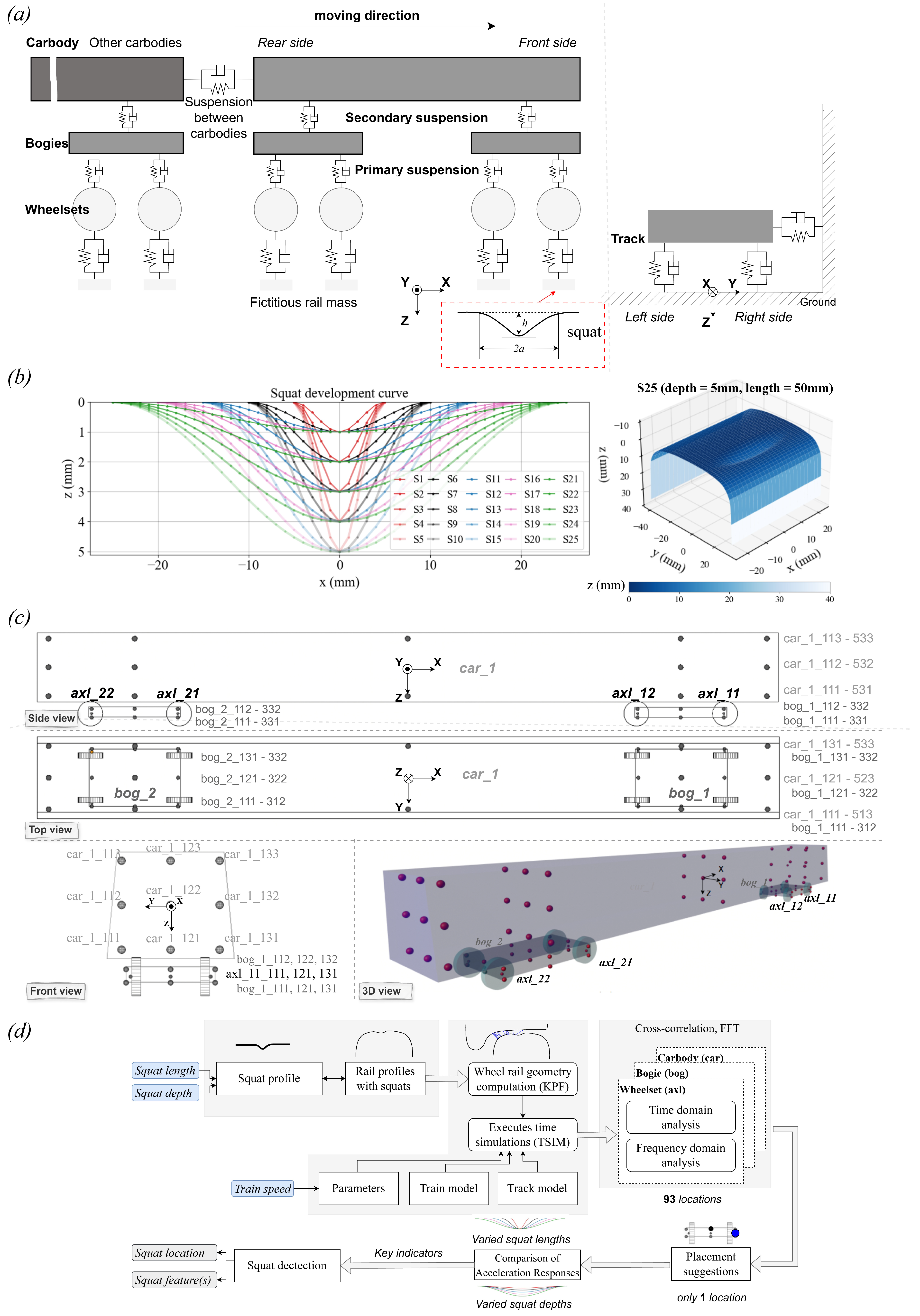
The train model used is one NSB Class 73 train with four carriages as Figure 2a modeled in commercial multibody simulation software GENSYS. Each carriage model includes primary and secondary suspensions with spring-damper elements that connect four wheel sets, two bogies, and one car body. It has six degrees of freedom (DOFs): X, Y, Z, roll, pitch, and yaw. The entire train-track model was developed based on a typical moving track model, which is a mass–spring–damper systems coupled to each wheel set. For each wheel profile and rail cross-section combination, the wheel–rail contact geometry is precomputed using the GENSYS module KPF (Kontaktpunktsfunktion, Contact Point Function in Swedish). The tabulated contact geometry functions are then interpolated for use in subsequent time integration analyses. Hertzian contact theory is applied to obtain linearized normal contact stiffness, while the tangential contact problem is solved using the FASTSIM algorithm (a simplified theory based on Kalker) [34]. The function wr_coupl_pe4 was applied to allow for a maximum of two different contact surfaces to be in contact simultaneously for each wheel. The definition and additional information on these functions and modules can be found in the GENSYS user manual [33]. The rail profile is 60E1, and the wheel set profile is ENS1002t32.5. Table 1 provides the other primary parameters of the train-track model, along with the eigen frequencies of four typical eigen modes [35].

2.2. Squat Model

Consider geometric description [21,23,36], rail squats are modeled on the left rail using Equation (1).
z s ( x , y , y 0 ) = h 2 1 + cos π x a 2 + y y 0 b 2 , x , y x , y : x a 2 + y y 0 b 2 1
where z s , x, y represent the vertical, longitudinal, and lateral coordinates while y 0 is denotes the lateral coordinate of the squat center. h is the squat depth at the squat center, a and b are the half-length and half-width of the squat, respectively. Mathematically, a and b correspond to the longitudinal and lateral semi-axes of the elliptical projection of the dimple on the rail surface.
Our preliminary investigation suggests that variations in squat width and its position along the lateral and longitudinal directions have a very marginal effect on the train’s vertical acceleration compared to squat depth and length. Here, the wear condition is ignored, and the assumption is that the squat occurred within the moving contact patch, where y 0 is 10 mm and b is 10 mm. To evaluate the correlation between the squat features (depth and length) and optimal accelerometer placement, 51 2D profiles were configured with 1 mm intervals for every squat case. The range of squat depth h spans from 1 to 5 mm, and the length 2 a ranges from 10 mm to 50 mm. These squat cases are named as S n (where n = 1 , 2 , , 25 ) with n = h + ( a 10 ) 2 where h { 1 , 2 , 3 , 4 , 5 } and a { 5 , 10 , 15 , 20 , 25 } . For any squat case, each 2D profile of the rail squat is simulated to act on the rail surface using a given defect-free rail 2D profile, ensuring accuracy in the YoZ plane. Each sample point on the defect-free rail profile is matched with a corresponding point on the squat profile to maintain geometric precision. The kpf function calculates the wheel–rail contact geometry based on the wheel profile and the rail profile with the simulated squat. The fine longitudinal interval between squat 2D profiles further improves the reliability of the wheel–rail contact simulation in the driving direction especially at high train speeds. Figure 2b illustrates all these squats with markers representing the 51 profiles, along with a 3D visualization of the left rail in the squat case S 25 , where the depth is 5 mm and the length is 50 mm.

2.3. Analysis

To identify the optimal installation locations for accelerometers on trains to achieve the highest sensitivity correlation between acceleration and squat features (depth and length). This means that placing sensors in these locations facilitates easier and more accurate squat feature detection. The naming convention follows the pattern O_N_XYZ, representing the object and serial number (OSN) from the front side, as well as the OSN from the positive direction along the x, y, and z axes. There are 93 locations, comprising 5 × 3 × 3 = 45 (car_1_111-car_1_533) for the car body, 2 × 3 × 3 × 2 = 36 (bog_1_111-bog_2_332) for the bogies, and 4 × 1 × 3 × 1 = 12 (axl_11_111-axl_22_131) for the wheel sets, see Figure 2c. More coordinate details can be found in Table A1. The sampling frequency rate is set at 100 kHz, to ensure that it is able to capture rail profiles variation under train speed of 160 km/h.
Pearson’s linear correlation coefficient ( P corr ) is selected as the cross-correlation function to measure the correlation between acceleration signals under varying squat cases on rails and the S1 case (depth = 1 mm and length = 10 mm). The resulting value falls within the range [−1, 1], where 1 indicates perfect correlation and −1 indicates perfect anti-correlation. The computation between two acceleration signals X and Y is defined as Equation (2).
P corr ( X , Y ) = c o v ( X , Y ) D X D Y = n i = 1 ( x i x ¯ ) ( y i y ¯ ) n i = 1 ( x i x ¯ ) 2 n i = 1 ( y i y ¯ ) 2
where c o v ( X , Y ) is the covariance of X and Y; x ¯ and y ¯ are the mean values, respectively; D X and D Y are the variances. A value of zero indicates a complete lack of correlation, suggesting that a significant change in the acceleration signal is likely due to a change in squat features, making it easier to detect. The computation range along the longitudinal axis is from −25 mm (covering the largest size of squat) to 125 mm (where the accelerations are almost damped out), with the origin at the center of squat cases.
Figure 2d highlights the analysis process. It produces squat profiles according to the given length and depth. After integrating the squats and rail profiles, using GENSYS to perform wheel–rail geometry computation (kpf) and time simulations (TSIM), it analyzes the installation locations of the wheel sets, bogies, and car body. The sensitivity indicators include P corr and peak values of amplitudes after Fast Fourier Transform (FFT). After evaluating P corr under various train speeds for all squat cases, an optimal installation location could be found, together with recommended train speeds. Furthermore, a detailed comparison of the acceleration response at this selected location is conducted for varying squat lengths and depths individually using typical cases. This comparison aims to identify potential key indicators from the responses that exhibit stronger correlations with rail squat characteristics. As a result, These indicators can support squat detection by pinpointing locations and determining squat geometry features.

3. Results

Section 3.1 identified the optimal accelerometer placements on the car body, bogie, and wheel set by evaluating the cross-correlation indicator P corr in 93 selected locations. Section Train Speed Variation presented a sensitivity analysis of the correlation between squat features and acceleration responses under varying train speeds, focusing on the identified positions for the car body, bogie, and wheel set. Among these, the wheel set emerged as the most suitable location for accelerometer installation. Section 3.2 further provided acceleration signals generated by squat length and depth variations independently in detail. The results encompassed comparative assessments of time-domain and frequency-domain responses, peak acceleration magnitudes, and delay offsets across five representative train speeds.

3.1. Optimal Accelerometer Placement

The experiments found that the P corr values are similar for different squat depths, indicating little influence on the changes in accelerations. Figure 3a illustrates that the accelerometer values are generally more sensitive at lower speeds (20 km/h) compared to higher speeds (160 km/h and 80 km/h). Among the optional positions, the lateral center (axl_11_121) and left (axl_11_131) of the front wheel set show notable sensitivity. Figure 3b provides the vertical displacements of the leading wheel set under all squat cases for 20 km/h. The dotted lines represent the center of squats, while five horizontal lines above them indicate squat length. The length of squats directly influences the wavelength, and all the peaks occur after the zero location. Meanwhile, smaller squat lengths such as 10 mm, 20 mm, and 30 mm also affect the amplitude. The change of displacements damped out after approximately 0.1 m. Figure 3c–e show that the largest squat case, S25, always has the smallest P corr values, indicating it is the most sensitive. Due to the primary and secondary suspensions, the vertical acceleration is generally attenuated in a ratio of 10 (wheel set):1 (bogie):0.05 (car body) and exhibits a progressive time delay from the wheel set to the car body. For bogies, the lateral left and center exhibit the highest sensitivity, the same as for the wheel sets. For the car body, the values are very close along the lateral directions. The lateral left (blue) locations show the largest amplitudes in the time domain and retain more frequency features in the response spectra. Therefore, axl_11_131, bog_1_131, and car_1_131 are optimal installation locations, confirming earlier contact positions in the x-axis and other rules [32].

Train Speed Variation

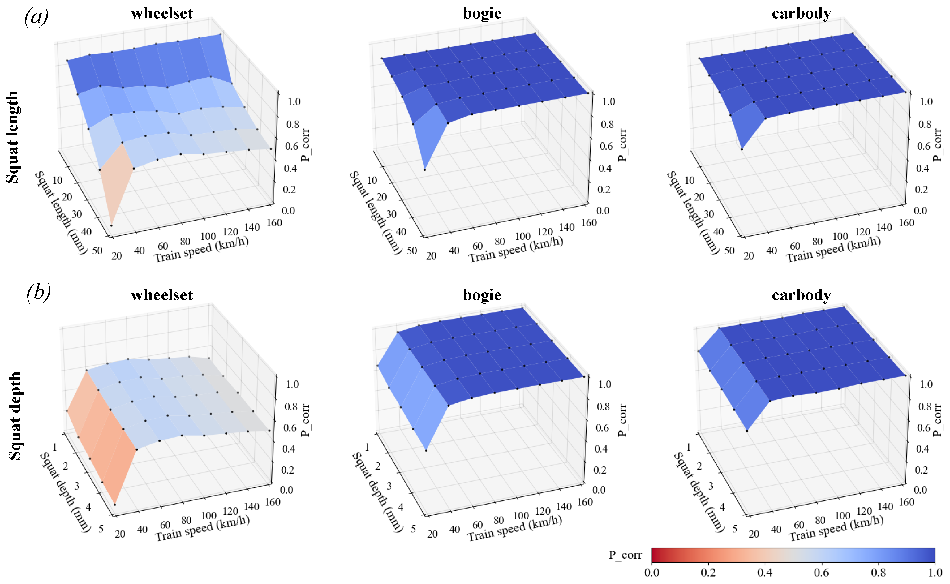
To discuss the effect of train speeds on the optimal installation locations (axl_11_131, bog_1_131, and car_1_131) on the wheel set, bogie, and car body, correlation sensitivity analysis was executed for squat length and squat depth separately. Figure 4 shows that the sensitivity of squat length significantly outweighs that of squat depth concerning the correlation of accelerations in the car body, bogie, and wheel set. At 20 km/h, the highest sensitivity is observed in Figure 4a. Increasing the train speed reduces the sensitivity of car body and bogie accelerometers greatly, particularly beyond 40 km/h. For trains requiring higher speeds, it is recommended to install accelerometers on the wheel set to capture maximum sensitivity, with a suggested speed of 160 km/h. Figure 4b illustrates that the influence of squat depth is significantly constrained even with a squat length of 50 mm. Therefore, detecting squat depth proves challenging regardless of the train speed. Additionally, the train speed between 160 km/h and 100 km/h shows little effect on the results. Given that our primary goal is squat detection at regular operational speeds, the wheel set acceleration exhibits a stronger correlation with changing squat features (indicated by lower P c o r r values) across the speed range than the accelerations measured on the bogie and car body. The more pronounced variability observed on the bogie and car body at 20 km/h is less representative in practice, as trains cannot routinely operate at such low speeds only for squat inspection. For these reasons, axl_11_131 on the wheel set is chosen as the installation location for the subsequent analysis.

3.2. Acceleration

The optimal accelerometer placement method identified that the accelerometer installed on the first wheel set exhibited lowest P corr values. Lower P corr (highlighted in red) indicates that deviations in squat geometry (length and depth) induce more detectable variations in acceleration signals. This section analyzes comparative cases for squat length and depth across five representative speeds: 20, 40, 60, 80, and 160 km/h. Data for intermediate speeds (100, 120, and 140 km/h) exhibited transitional trends between the 80 km/h and 160 km/h benchmarks and were omitted to streamline the discussion.

3.2.1. Squat Length

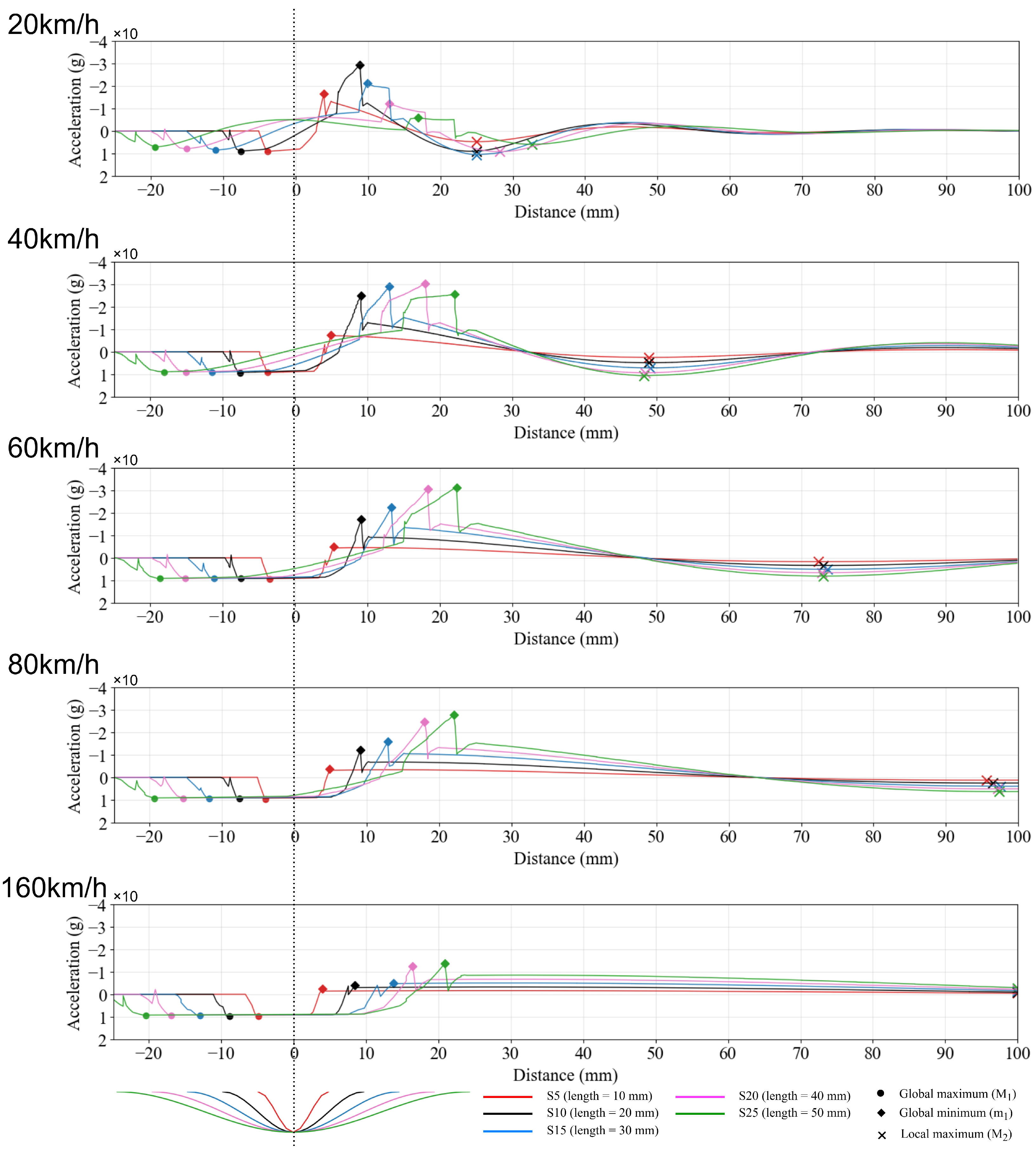
Figure 5 depicts acceleration curves across train speeds (20–160 km/h) for five squat length cases (S5–S25: 10–50 mm) at a fixed squat depth of 5 mm. All curves exhibit a consistent waveform: a rapid ascent to a global maximum acceleration M 1 (points marked as circles), followed by a reversal to a minimum m 1 (diamonds), a secondary rise to a local maximum M 2 (crosses), and subsequent damped oscillations toward zero. At 20 km/h, M 1 decreases marginally from 9.19 g (S5) to 9 g (S10), then undergoes a step-wise decline to 7.11 g (S25), reflecting a minimum 5% relative reduction per 10 mm increase in squat length, which is emphasized in Figure 6b. This sensitivity diminishes markedly at speeds higher than 40 km/h, variations fall below 0.5% between 9.29 g (S10) and 9.22 g (S15). Beyond 60 km/h, the M 1 curves in Figure 6b flatten, showing only minor variations (<0.1%), such as 9.23 g (S15) and 9.22 g (S20). The highest recorded acceleration M 1 (9.84 g) occurs at 160 km/h for the shortest squat length (10 mm, S5). Notably, in Figure 6c, the y-values for M 1 (circles) decrease step-wise from approximately −4 mm to −20 mm as the x-values increase, across all listed train speeds. This means the longitudinal positions of M 1 are independent of train speed, consistently localized near the leading edge and before the center of the squat.
The minimum accelerations m 1 demonstrate greater magnitudes and variability approximately 3 times as large as the global maximum accelerations M 1 , with −29.3 g (S10) at 20 km/h and −30.5 g (S20) at 40 km/h. The extreme m 1 among all curves is −31.3 g (S25) at 60 km/h. Above 60 km/h, all minimum accelerations (diamonds) in Figure 6b decrease in absolute value, but the differences in amplitude are irregular, suggesting no clear correlation. In contrast to M 1 , the y-values for m 1 (diamonds) in Figure 6c increase step-wise with rising x-values. This suggests that the longitudinal positions of m 1 remain fixed after the squat center and near its trailing boundary, regardless of various train speeds.
The local maximum accelerations M 2 following minimum accelerations m 1 are pronounced at speeds below 80 km/h (e.g., 10.6 g for S15 at 20 km/h). Beyond 40 km/h, these values exhibit linear correlation with squat length. For example, M 2 increases step-wise by ∼2.5 g from S5 to S25 (2.51 g, 4.86 g, 7.18 g, 9.34 g, 10.7 g); while their longitudinal positions vary minimally, they display linear dependence on train speed rather than squat characteristics. The averages of these longitudinal positions are 25 mm (20 km/h), 49 mm (40 km/h), 73 mm (60 km/h), 97 mm (80 km/h). Therefore, the longitudinal positions M 2 (crosses) are approximately 250 mm for 160 km/h. However, they are plotted at the maximum boundary of 100 mm due to the limited x-axis range in the figures.
Figure 6a presents frequency-domain spectral analysis, revealing that above 40 km/h, frequency curves exhibit speed-dependent linear relationships with squat length. At 20 km/h, mid-to-high frequency (100–500 Hz) squat-related components dominate, while 40 km/h exhibits distinct separation between low-frequency (<100 Hz) and mid-to-high frequency features, facilitating differentiation of acceleration signals. Beyond 60 km/h, spectral amplitude convergence renders frequency-domain detection of squat-related signals increasingly challenging. Figure 6b plots the acceleration values of M 1 , m 1 , and M 2 . In general, M 1 (circles) exhibits smaller value differences across cases, except at 20 km/h, and shows no linear correlation with squat length for the 40 km/h and 60 km/h cases. On the contrary, m 1 (diamond) displays the largest value variations but has poor linear correlation at 20 km/h. Meanwhile, M 2 (crosses) demonstrates the best linear correlation with squat length among these three acceleration values, particularly at 40 km/h and 60 km/h. The corresponding longitudinal positions for accelerations are shown in Figure 6c, which exhibit clearer linear correlations. The values of M 1 (circles) and m 1 (diamonds) are symmetric about zero, and their separation increases linearly with squat length. M 2 (crosses) increases linearly with train speed but remain independent of squat length.

3.2.2. Squat Depth

Figure A1 presents acceleration curves for varying squat depths (S21–S25, 1–5 mm) at a fixed length of 50 mm; while S21 (red), S22 (black), and S25 (green) display clear differentiation, S23 (blue) and S24 (pink) are difficult to distinguish as they nearly overlap with S25 due to their similar acceleration profiles. All curves retain the characteristic pattern of a global maximum ( M 1 ), a global minimum ( m 1 ), and a local maximum ( M 2 ). At 20 km/h, peak acceleration ( M 1 ) increases from 6.33 g (S21) to 7.11 g (S23), representing a 3% difference (0.3 g absolute). However, this difference decreases to just 0.5% (0.04 g absolute) above 40 km/h, indicating a weakening correlation with depth as Figure A2b shows. Figure A2c indicates that the longitudinal positions of M 1 remain nearly constant, varying only by 1–2 mm, particularly for S23–S25. Minimum accelerations exhibit greater variability, with S24 reaching −31.4 g at 60 km/h, although the values for S23–S25 converge closely. Frequency analysis in Figure A2a confirms the similarity among S23–S25, while Figure A2b,c show weak correlation between squat depth and both acceleration magnitudes, as well as longitudinal positions.

4. Discussion

Based on the comparative analysis of acceleration results, Section 4.1 introduces a mechanism in general and three variations. Section 4.2 extends this discussion by evaluating six defined squat-related feature indicators, proposing a detection method for squat center and length, and providing a quantitative analysis of detection accuracy. Section 4.3 presents practical recommendations on three key aspects: squat width detection, sensor selection, and optimal train speeds for squat detection.

4.1. Mechanism

Although the vertical acceleration of the first wheel set exhibits distinct responses depending on the simulated squat depth and length, a general mechanism can be concluded based on shared characteristics among these responses. This section begins by analyzing how vertical acceleration reflects the dynamic response of the train traversing a squat defect, followed by a study of three critical influencing factors. Furthermore, corresponding wheel–rail contact analyses validate the identified mechanism through observations of contact point dynamics and contact area dimensions, supported by representative cases.

4.1.1. Acceleration Response

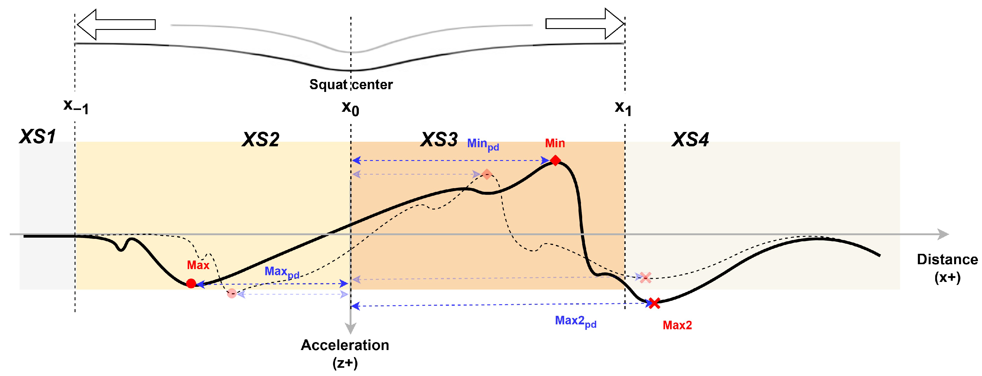
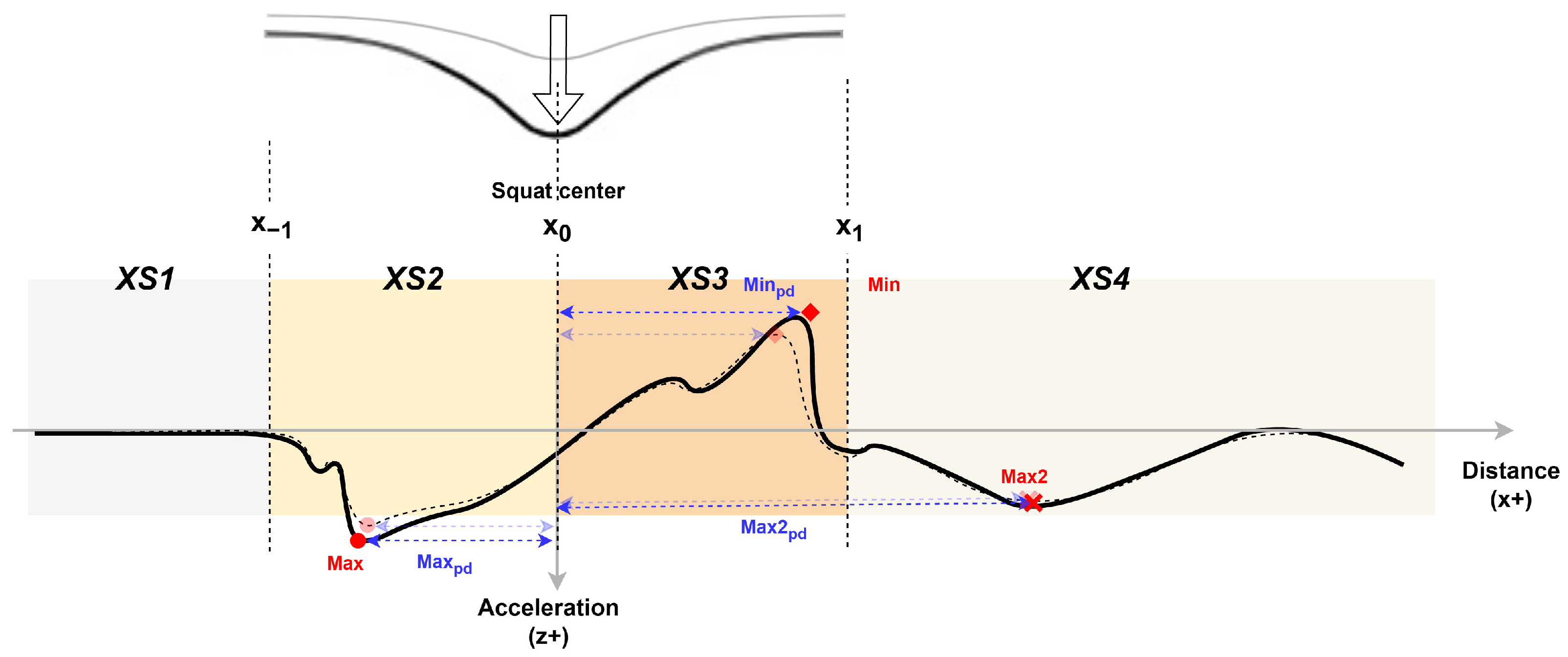
During the train’s traversal over a rail squat, three critical instants (specific moments) are identified based on the center point of the first wheel set center: entry into the squat (marked as x 1 ), alignment with the squat center ( x 0 ), and exit from the squat ( x 1 ), as illustrated in Figure 7. The process is further subdivided into spatial segments XS1–XS4. Segments XS2 and XS3 correspond to the wheel’s passage directly over the squat, where geometric features of the defect dominantly influence dynamic responses. In contrast, segment XS4 exhibits minimal correlation with squat geometry, as its behavior is governed by suspension system dynamics and train velocity after subsequent wheel sets traverse the defect.
Figure 7 illustrates the relationship between squat geometry, wheel–rail contact, and acceleration response. The squat geometry directly influences wheel–rail contact along the lateral contour of the rail surface, and the resulting contact forces generate the corresponding vertical acceleration. During the nominal conditions in segment XS1, there is only one contact point ( c p 1 ) for the left and right wheels. The force curves (highlighted in blue and purple) balance and support the entire weight of the load. During squat traversal in XS2 and XS3, c p 1 (acting in the positive z-direction) induces a global acceleration peak ( M 1 , acc ) due to wheel–rail contact. Meanwhile, transient two-contact interactions on the left rail ( c p 1 and c p 2 ) produce a secondary peak of reduced magnitude in regions where c p 2 forces (red) are present. After the maximum acceleration, both c p 1 and c p 2 contact forces diminish to zero, potentially leaving no contact points on the left wheel. If the train speed is sufficiently high, the train may travel a longer distance within this short period, resulting in a flat curve that occupies most of XS2. The primary peak is characterized by the point M 1 ( M 1 , acc , M 1 , pd ) where M 1 , acc denotes peak acceleration magnitude and M 1 , pd represents the phase delay relative to the squat center.
Following instant x 0 , diminishing squat displacement reverses the vertical dynamics, driving acceleration toward a negative z-direction in section XS3. This minimum reflects intensified restorative forces from the suspension system and prolonged c p 2 contact during the two-contact phase compared with XS2. It is named as m 1 ( m 1 , acc , m 1 , pd ) .
In XS4, the first wheel set exits the squat, initiating system rebalancing although subsequent wheel sets induce low-magnitude oscillations modulated by suspension damping. However, the acceleration signals are insufficient to resolve squat geometry. The first detectable post-exit acceleration peak, denoted M 2 ( M 2 , acc , M 2 , pd ) , emerges during this damped transient regime. Consequently, the sum of contact forces on the left wheel (grey) shapes the observed acceleration profile (black) (Figure 7).

4.1.2. Influencing Factors

The acceleration response to a rail squat is influenced by the geometry of the squat, rail and track properties, train characteristics, and various other factors. This section focuses on two parameters associated with the track-side geometry of the squat and the most critical train-side factor: train speed. Collectively, these factors exert the most significant influence on acceleration.
  • Squat Length
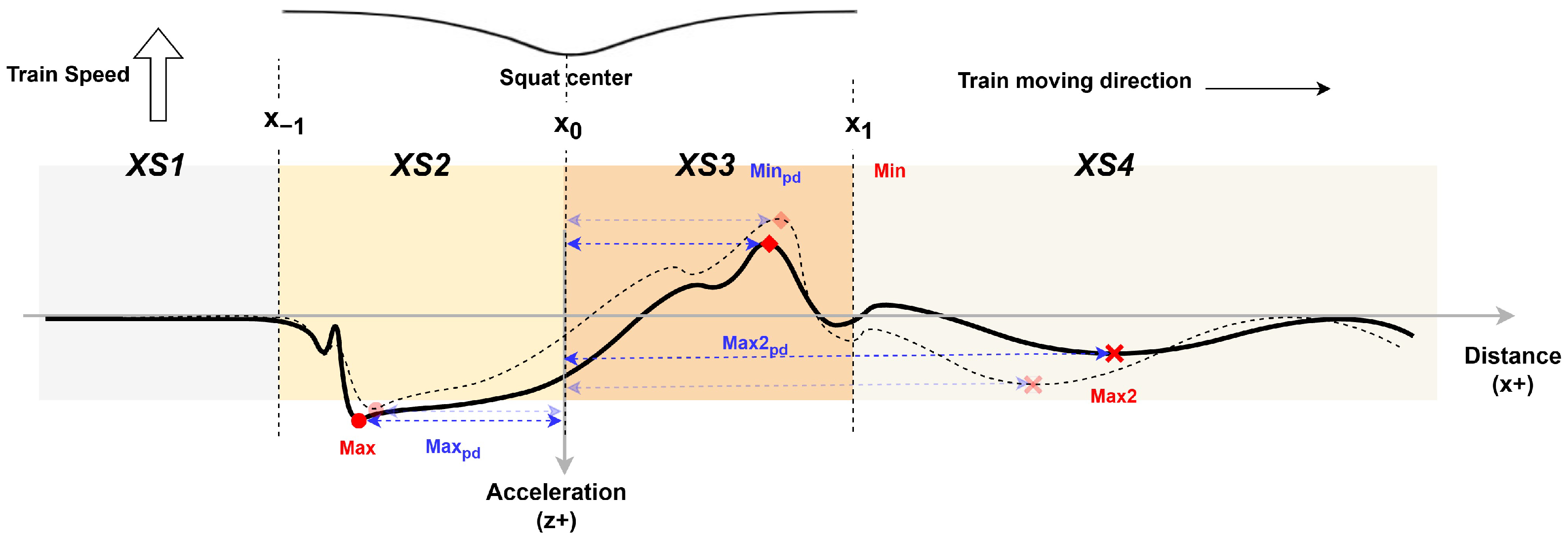
As squat length increases in Figure 8, the instants x 1 (entry) and x 1 (exit) shift proportionally. The distance phase delays M 1 , pd and m 1 , pd scale linearly with the squat length 2 a . Since the squat depth (several millimeters) is smaller relative to the wheel radius (hundreds of millimeters), the vertical acceleration peak M 1 , acc in segment XS2 shows little variation. In contrast, two-point contact conditions during squat traversal introduce sensitivity in m 1 , acc (segment XS3). The localization of m 1 , acc becomes challenging when the cp2 force undergoes significant variation over prolonged durations or occurs with the large time offset compared with cp1. Segment XS4 behavior correlates weakly with squat geometry but retains residual squat length-dependent effects in the direction of travel; while attenuated, M 2 , acc retains partial geometric information for defect characterization.
  • Squat Depth
The driving direction (longitudinal) is orthogonal to the formation and evolution of squat depth h, while vertical acceleration on the wheel set aligns with the direction of squat depth. Consequently, the dynamic wheel–rail contact conditions in the vertical and longitudinal directions correlates squat depth and vertical acceleration, particularly through changes in contact points and contact forces induced by varied squat depths. In this context, squat length and wheel radius affect the outcome as well.
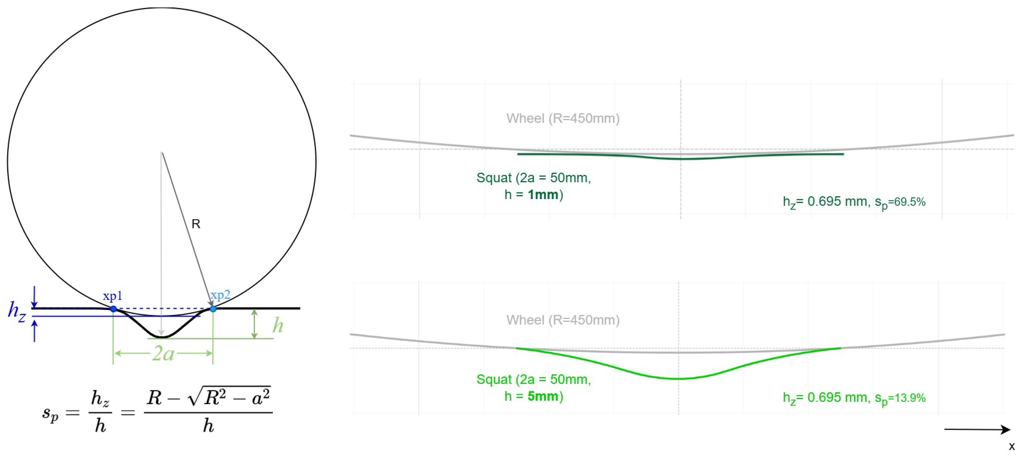
There are two contact points, x p 1 and x p 2 , when the first wheel set passes over the center of the squat. In this case, the parameter perceived squat depth h z is introduced, representing the difference in displacement between the bottom of the wheel and the line connect points x p 1 and x p 2 , as highlighted in Figure 9. The ratio of h z to h describes the sensitivity between acceleration and squat depth, given by the equation:
s p = h z h = R R 2 a 2 h
where R is the wheel radius, and h and 2 a represent the squat depth and length, respectively. The distance between x p 1 and x p 2 approximates the squat length 2 a since R > > h .
As squat depth varies, the instants x 1 (entry) and x 1 (exit) exhibit negligible temporal shifts if the squat length remains constant as Figure 10. Meanwhile, perceived squat depth h z tends to align more closely with the smaller actual squat depth. At lower train speeds, the duration of the one contact phase at x p 1 correlates with squat depth, as deeper squats exhibit steeper ramp curvatures, inducing faster changes in dynamic forces and acceleration. Consequently, the vertical acceleration peak M 1 , acc is more likely to correlate with squat length than with phase delay parameters.
  • Train Speed
When the train speed exceeds 120 km/h, it takes less than 1 ms to pass over a squat of 30 mm length. In such cases, the wheel may experience a very brief loss of contact after instant x 1 , effectively “flying over” the squat. Under these conditions, the squat depth has minimal influence, but the squat length can still be detected using the contact points contact on instants x 1 and x 1 , provided the sampling rate is sufficiently high (no less than 100 kHz). On the other hand, the wavelength in segment XS4 varies with train speed. For example, the phase delay M 2 , pd shifts proportionally with the train speed as Figure 11. Since the response of the suspension system is influenced by train speed, it is essential to analyze the accuracy of squat detection under different train speeds.

4.2. Squat Detection

The experimental findings reveal a strong correlation between acceleration response and squat geometry features. To investigate how this mechanism could enhance squat detection, Section 4.2.1 conducts a qualitative analysis of six variables: three peak vertical acceleration values and their corresponding longitudinal delay offsets, evaluated in the context of squat length and depth. Performance indicators showed higher sensitivity to variations in squat length than to squat depth. Building on these results, Section 4.2.2 and Section 4.2.3 propose a simplified linear correlation model to estimate the longitudinal squat center location and squat length using the two most sensitive variables. Validation experiments confirm that the estimation error remains within 2 mm, while the optimized relative accuracy exceeds 90% across all tested train speeds (20–160 km/h).

4.2.1. Qualitative Analysis

Section 4.1 described the response of six defined variables ( M 1 , acc , m 1 , acc , M 2 , acc , M 1 , pd , m 1 , pd , and M 2 , pd ) to the variations in squat length, squat depth, and train speed. Since they exhibit a certain degree of correlation with the targeted squat features, variables with stronger correlations may be selected as indicators for further squat detection after qualitative analysis. The classification framework categorizes the degree of correlation into three qualitatively distinct levels: Avoid (low effectiveness with no significant correlation, marked as ×), Conditional (moderate effectiveness with a non-linear correlation, △), and Optimal (high effectiveness with a clear linear correlation, O). The correlation results, based on these criteria and experimental findings, are summarized in Table 2 and Table 3. Although vertical vibration weakens, particularly at speeds above 80 km/h, the phase delay variables are significantly more stable than the highly susceptible amplitude variables. As shown in Table 2, when analyzing various squat lengths, M 2 , acc exhibits a stronger correlation compared to M 1 , acc and m 1 , acc . Both M 1 , pd and m 1 , pd demonstrate optimal performance across all train speeds. In contrast, M 2 , pd should be avoided, as no correlation was found with squat length. Table 3 shows that none of the variables demonstrate optimal effectiveness under all conditions, but m 1 , acc , M 2 , acc , m 1 , pd , and M 1 , pd outperform the other two variables in low train speed scenarios.

4.2.2. Squat Center

Among the acceleration and phase delay variables, the midpoint between the M 1 and m 1 peaks is most closely correlated with the squat center. We define the estimated position of squat center on the longitude direction as
x 0 ^ = M 1 , pd + m 1 , pd 2 ,
and the relative accuracy as
Δ x 0 = 1 x 0 ^ x 0 2 a × 100 % ,
in terms of varied squat lengths. x 0 is zero because the simulated squat centers are defined as the origin of the x-axis. The results are shown as Table 4. Ignoring the abnormal values (highlighted in red), the estimated positions range from −1.11 mm to 2 mm. Meanwhile, the minimum relative accuracy is 90.85%.

4.2.3. Squat Length

The difference between the delay offset values m 1 , pd and M 1 , pd is highly correlated with the squat length. The estimated squat length is defined as
x 2 a ^ = k a ( m 1 , pd M 1 , pd ) ,
when k a is a correction factor to improve estimation accuracy. For example, in a known theoretical case such as S1, the factor k a can be calculated as 2 a m 1 , pd M 1 , pd . The relative accuracy is expressed as
Δ x 2 a = 1 x 2 a ^ 2 a 2 a × 100 % ,
which quantifies the accuracy of the squat length estimation. The results are summarized in Table 5 with no correction ( k a = 1 ). Except for the worst-case scenario at a train speed of 20 km/h, all other cases exhibit a higher relative accuracy over 80% with linear dependence on the squat length. Furthermore, the estimated squat length approximates 80% of the actual squat length.
By calculating k a for the case S1 at 20 km/h: k a = 2 a m 1 , pd M 1 , pd = 10 mm 5 mm ( 3.33 mm ) 1.20 , the revised x 2 a ^ increases from 7.78 mm to 9.34 mm, and Δ x 2 a improves from 77.8% to 93.4%. The overall average relative accuracy Δ x 2 a exceeds 95%.

4.3. Suggestions

4.3.1. Squat Width Detection

Squat width, denoted as 2b in Equation (1) is a critical geometric parameter in railway squat characterization except for length and depth. Unlike squat length and depth, which develop along the longitudinal (x-axis) and vertical (z-axis) directions, squat width varies perpendicularly to the lateral-vertical (XoZ) plane. This plane is particularly sensitive to vertical acceleration signals captured by track-mounted accelerometers, as train motion occurs along the x-axis. To evaluate the influence of squat width on sensor performance, optimal sensor placement was also executed across variations in train speed (20–160 km/h) and squat widths (10–50 mm). Results indicate that squat width alone has very little impact on vertical acceleration amplitudes, particularly at high speeds (>100 km/h), where its individual sensitivity ranks between that of squat length and depth but aligns more closely with depth. Notably, squat width is strongly correlated with squat length during defect progression, as both parameters scale with mechanical wear. To isolate and emphasize the effects of individual squat features in this study, squat width was held constant at a representative value (e.g., 20 mm), ensuring controlled and generalizable analysis.

4.3.2. Sensor Selection

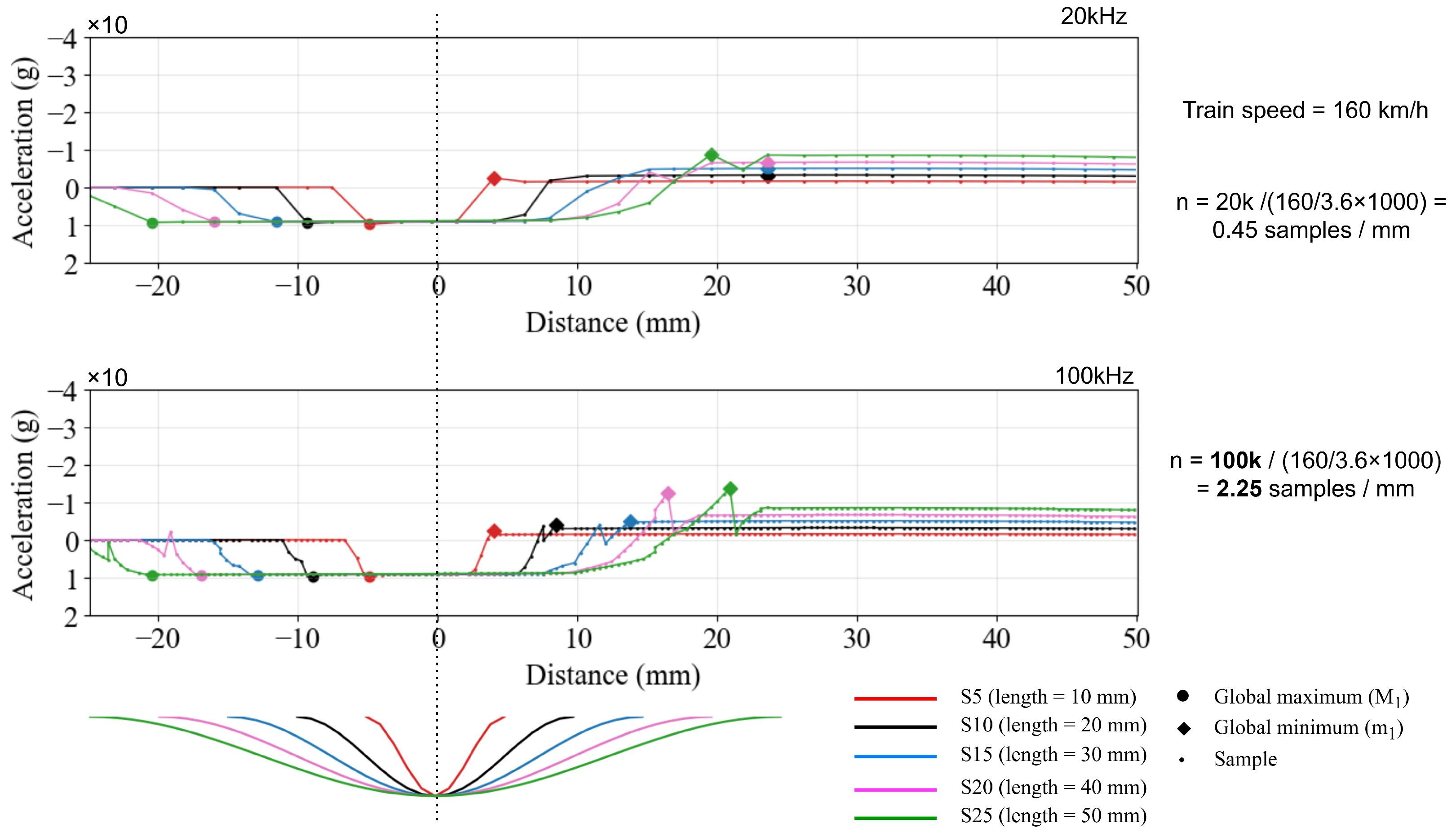
The selection of acceleration sensors depends on critical technical parameters such as measurement range, sensitivity, resolution, and sampling frequency because these factors directly influence both system accuracy and cost. Sensitivity, quantified in mV/g, reflects the sensor’s theoretical accuracy in converting mechanical acceleration to an electrical signal within a standard 0–10 V range. Relative measurement accuracy is inversely proportional to the selected measurement range, meaning a wider range (e.g., ±500 g) reduces resolution, whereas a narrower range enhances precision. The sampling frequency is governed by the minimum of the sensor’s inherent sampling capability and the configurable data acquisition (DAQ) channel rate. In practice, the DAQ rate is often intentionally limited to reduce computational and storage demands. Based on this study’s findings, a measurement range of ±50 g is recommended to encompass observed acceleration peaks (−31.4 g to 10.7 g), with a resolution ≥0.01 g to ensure detection of squat features. Sampling frequencies of 100 kHz and 20 kHz are advised for train speeds ≥60 km/h and <60 km/h, respectively; while commercially available accelerometers (Table 6) generally satisfy resolution and range requirements, their sampling frequencies are often limited to 20 kHz, which risks undersampling at higher train speeds. As illustrated in Figure 12, a 20 kHz sampling rate may fail to capture acceleration peaks with less sample points every millimeter introducing positional errors of 20–50 mm in squat center and length determination. Conversely, 100 kHz sampling improves accuracy but increases data communication and storage burdens unless redundant data is filtered. To address this trade-off, a two-stage strategy is proposed: initial squat detection at 20 kHz for preliminary center identification, followed by localized 100 kHz sampling (e.g., ±500 mm around detected regions) to refine squat length measurements if positional offsets occur.

4.3.3. Optimal Train Speeds

The Roger 1000, a standard Norwegian maintenance train, operates at 40 km/h with a typical speed range of 0–130 km/h and a maximum of 160 km/h, while passenger trains exhibit a normal operating range of 130–145 km/h (maximum 210 km/h). To mitigate sensor sampling limitations at high speeds, a unified test range of 20–160 km/h was selected to cover both train types. Section Train Speed Variation revealed squat length and depth are most sensitive at 20 km/h across all sensor positions (wheel set, bogie, car body), meaning maintenance vehicle is recommended to operate at 20–40 km/h for accurate squat detection. Acceleration signals stabilize into consistent patterns above 80 km/h, with squat center detection showing uniform error distribution around ground-truth values at >120 km/h and squat length accuracy improving marginally above 100 km/h (Table 4). Consequently, a speed range of 80–120 km/h is recommended to balance robust squat detection with operational practicality, ensuring reliable defect identification while accommodating typical service conditions.

4.4. Limitations

In this paper, the parameter space is constrained by a limited set of discrete values for train speeds, accelerometer locations, and squat geometric features. The methodology employs an optimal sensor placement to quantitatively decide accelerometer installation locations within defined 93 potential locations. This process identified three optimal locations, and ultimately to a single optimal position on the wheel set. The train speed is set between 20 km/h and 160 km/h, with intervals of 20 km/h. The behavior in the low-speed range (20–40 km/h) exhibited significantly greater sensitivity compared to other speeds. The qualitative analysis is utilized for exploring the mechanism and rest of methodology relied on constrained quantitative comparisons. Given the scope of this paper, only the most representative results are presented.
On the other hand, this study focuses on detecting a single rail squat located on one side of the track. Experimental results identified the optimal accelerometer location on the left wheel set, based on the lowest P corr value; while a squat on the right rail would shift the optimal location to the right wheel set, the performance difference is marginal as the underlying mechanism of correlation remains the same. In practice, determining the position and severity of a squat is more critical than identifying its exact side of the rail. It should be noted that factors such as curve radius, track inclination, track stiffness and the profiles of wheels and rails may also influence the correlation sensitivity in real-world scenarios, even though these factors are typically treated as constants during a single simulation case. The train’s eigen frequencies and modes (Table 1) were not emphasized in the analysis because the experimental data contained limited information in those frequency bands. In practice, sensor selection must also consider physical dimensions and connection methods.
Regarding the squat model, the longitudinal interval of the squat profile is set to 1 mm, with a sampling rate of 100 kHz for the simulation. No significant differences were observed when smaller intervals or higher sampling rates were used. To improve squat modeling, a direct approach is to incorporate highly accurate squat profiles obtained from real-world measurements. Another potential improvement involves refining the squat modeling functions, such as representing squats with two pits of different sizes instead of a single large pit. This method more accurately replicates the squat shape, especially for moderate and severe squats.

5. Conclusions

This paper employed the multibody simulation software GENSYS to model train dynamics as a passenger train traversed simulated squats on a straight track. The analysis focused on determining the optimal placement of accelerometers for distinguishing between squats of varying depths and lengths. Frequency-domain tools, including the cross-correlation function ( P corr ), were utilized to assess the effects of train speed and squat characteristics on detection accuracy. The key findings of the study are summarized as follows:
  • Sensor Placement and Train Speed: Accelerometers positioned on the first wheel set near the wheel–rail contact points exhibited the highest sensitivity to squat features. This supports the widely accepted principle in current research that sensor placement near the wheel–rail interface enhances detection accuracy. The analysis of results showed lower train speeds such as 20 km/h can induce a more pronounced correlation between squat features and vertical acceleration, especially when sensors were installed on the car body.
  • Correlation Mechanism: A generalized mechanism linking squat geometry (length and depth) to vertical acceleration responses was established, despite variations in patterns due to changes in train speed and squat geometry. This mechanism, including three critical instants and four distinct response segments, concluded six evaluative indicators. These indicators are correlated with the train speed and squat geometry parameters to different degrees.
  • Squat Detection Performance: Squat length exhibited the highest sensitivity compared to depth and width in defect identification. Leveraging two of the six evaluative indicators defined in the correlation mechanism, the proposed method successfully localized squats and quantified squat length in case studies, achieving 90% accuracy across all tested train speeds. This speed-invariant reliability underscores the found mechanism and the introduced method’s robustness and practical applicability for real-world rail maintenance.
To advance this work, future research should expand to the identification of several squats on a rail, the refinement of simulation models to better represent squat development, and validation within a more complex parameter space and real squat cases. The findings of this paper provide valuable guidance for optimizing accelerometer placement to enhance the effective detection of squat features. The experimental results by labeled squat feature values, can serve as a robust foundational dataset for training and developing machine learning models.

Author Contributions

Conceptualization, Z.H. and A.L.; methodology, Z.H. and A.L.; software, Z.H.; validation, Z.H.; formal analysis, Z.H. and A.L.; investigation, Z.H.; resources, Z.H. and A.L.; data curation, Z.H.; writing—original draft preparation, Z.H.; writing—review and editing, Z.H. and A.L.; visualization, Z.H.; supervision, A.L. All authors have read and agreed to the published version of the manuscript.

Funding

This research received no external funding.

Data Availability Statement

The technical data of the train model are not publicly available due to commercial reasons. The other raw data supporting the conclusion of this article will be made available by the authors on request, without undue reservation.

Acknowledgments

The original pictures of the rail squats shown in Figure 1 are provided by Thomas Vatn Bjørge/Bane NOR, Vestfoldbanen, Norway.

Conflicts of Interest

The authors declare no conflicts of interest.

Abbreviations

The following abbreviations are used in this manuscript:
NDTNon-Destructive Testing
RCFRolling Contact Fatigue
S&CSwitches and Crossings
ABAAxle Box Acceleration
KPFKontaktpunktsfunktion (Swedish), Contact Point Function
DOFDegree of Freedom
TSIMTime simulation
OSNObject and Serial Number
FFTFast Fourier Transform
DAQData Acquisition

Appendix A

The appendix includes more details of experiments.
Table A1. The relative coordinates of all monitoring points with the car body center as the origin.
OSNCoordinates (X,Y,Z) Unit: MeterOSNCoordinates (X,Y,Z) Unit: Meter
car_1_111 ( 12.8 , 1.1 , 1.1 ) bog_1_111 ( 11.1 , 1 , 1.65 )
car_1_121 ( 12.8 , 0 , 1.1 ) bog_1_121 ( 11.1 , 0 , 1.65 )
car_1_131 ( 12.8 , 1.1 , 1.1 ) bog_1_131 ( 11.1 , 1 , 1.65 )
car_1_112 ( 12.8 , 1.1 , 0.0 ) bog_1_112 ( 11.1 , 1 , 1.3 )
car_1_122 ( 12.8 , 0 , 0.0 ) bog_1_122 ( 11.1 , 0 , 1.3 )
car_1_132 ( 12.8 , 1.1 , 0.0 ) bog_1_132 ( 11.1 , 1 , 1.3 )
car_1_113 ( 12.8 , 1.1 , 1.1 ) bog_1_211 ( 9.5 , 1 , 1.65 )
car_1_123 ( 12.8 , 0 , 1.1 ) bog_1_221 ( 9.5 , 0 , 1.65 )
car_1_133 ( 12.8 , 1.1 , 1.1 ) bog_1_231 ( 9.5 , 1 , 1.65 )
car_1_211 ( 9.5 , 1.1 , 1.1 ) bog_1_212 ( 9.5 , 1 , 1.3 )
car_1_221 ( 9.5 , 0 , 1.1 ) bog_1_222 ( 9.5 , 0 , 1.3 )
car_1_231 ( 9.5 , 1.1 , 1.1 ) bog_1_232 ( 9.5 , 1 , 1.3 )
car_1_212 ( 9.5 , 1.1 , 0.0 ) bog_1_311 ( 7.9 , 1 , 1.65 )
car_1_222 ( 9.5 , 0 , 0.0 ) bog_1_321 ( 7.9 , 0 , 1.65 )
car_1_232 ( 9.5 , 1.1 , 0.0 ) bog_1_331 ( 7.9 , 1 , 1.65 )
car_1_213 ( 9.5 , 1.1 , 1.1 ) bog_1_312 ( 7.9 , 1 , 1.3 )
car_1_223 ( 9.5 , 0 , 1.1 ) bog_1_322 ( 7.9 , 0 , 1.3 )
car_1_233 ( 9.5 , 1.1 , 1.1 ) bog_1_332 ( 7.9 , 1 , 1.3 )
car_1_311 ( 0 , 1.1 , 1.1 ) bog_2_111 ( 7.9 , 1 , 1.65 )
car_1_321 ( 0 , 0 , 1.1 ) bog_2_121 ( 7.9 , 0 , 1.65 )
car_1_331 ( 0 , 1.1 , 1.1 ) bog_2_131 ( 7.9 , 1 , 1.65 )
car_1_312 ( 0 , 1.1 , 0.0 ) bog_2_112 ( 7.9 , 1 , 1.3 )
car_1_322 ( 0 , 0 , 0.0 ) bog_2_122 ( 7.9 , 0 , 1.3 )
car_1_332 ( 0 , 1.1 , 0.0 ) bog_2_132 ( 7.9 , 1 , 1.3 )
car_1_313 ( 0 , 1.1 , 1.1 ) bog_2_211 ( 9.5 , 1 , 1.65 )
car_1_323 ( 0 , 0 , 1.1 ) bog_2_221 ( 9.5 , 0 , 1.65 )
car_1_333 ( 0 , 1.1 , 1.1 ) bog_2_231 ( 9.5 , 1 , 1.65 )
car_1_411 ( 9.5 , 1.1 , 1.1 ) bog_2_212 ( 9.5 , 1 , 1.3 )
car_1_421 ( 9.5 , 0 , 1.1 ) bog_2_222 ( 9.5 , 0 , 1.3 )
car_1_431 ( 9.5 , 1.1 , 1.1 ) bog_2_232 ( 9.5 , 1 , 1.3 )
car_1_412 ( 9.5 , 1.1 , 0.0 ) bog_2_211 ( 11.1 , 1 , 1.65 )
car_1_422 ( 9.5 , 0 , 0.0 ) bog_2_221 ( 11.1 , 0 , 1.65 )
car_1_432 ( 9.5 , 1.1 , 0.0 ) bog_2_231 ( 11.1 , 1 , 1.65 )
car_1_413 ( 9.5 , 1.1 , 1.1 ) bog_2_212 ( 11.1 , 1 , 1.3 )
car_1_423 ( 9.5 , 0 , 1.1 ) bog_2_222 ( 11.1 , 0 , 1.3 )
car_1_433 ( 9.5 , 1.1 , 1.1 ) bog_2_232 11.1 , 1 , 1.3 )
car_1_511 ( 12.8 , 1.1 , 1.1 ) axl_11_111 ( 10.85 , 1 , 1.5 )
car_1_521 ( 12.8 , 0 , 1.1 ) axl_11_121 ( 10.85 , 0 , 1.5 )
car_1_531 ( 12.8 , 1.1 , 1.1 ) axl_11_131 ( 10.85 , 1 , 1.5 )
car_1_512 ( 12.8 , 1.1 , 0.0 ) axl_12_111 ( 8.15 , 1 , 1.5 )
car_1_522 ( 12.8 , 0 , 0.0 ) axl_12_121 ( 8.15 , 0 , 1.5 )
car_1_532 ( 12.8 , 1.1 , 0.0 ) axl_12_131 ( 8.15 , 1 , 1.5 )
car_1_513 ( 12.8 , 1.1 , 1.1 ) axl_21_111 ( 8.15 , 1 , 1.5 )
car_1_523 ( 12.8 , 0 , 1.1 ) axl_21_121 ( 8.15 , 0 , 1.5 )
car_1_533 ( 12.8 , 1.1 , 1.1 ) axl_21_131 ( 8.15 , 1 , 1.5 )
axl_22_111 ( 10.85 , 1 , 1.5 )
axl_22_121 ( 10.85 , 0 , 1.5 )
axl_22_131 ( 10.85 , 1 , 1.5 )
Figure A1. Measured acceleration response for five squat depths cases (S21–S25: 1–5 mm) under train speeds (20, 40, 60, 80, and 160 km/h). The dotted line indicates the longitudinal center of the squats.
Infrastructures 10 00313 g0a1
Figure A2. Acceleration analysis for five squat depths cases (S21–S25: 1–5 mm) under train speeds (20, 40, 60, 80, and 160 km/h): (a) Frequency-domain response; (b) Time-domain extrema ( M 1 : global maximum; m 1 : global minimum; M 2 : local maximum); (c) Phase delay characteristics ( M 1 , m 1 , M 2 ).
Infrastructures 10 00313 g0a2

References

  1. The Organisation for Economic Co-operation and Development (OECD). Rail infrastructure maintenance spending. In Proceedings of the International Transport Forum, Leipzig, Germany, 21–24 May 2024. [Google Scholar]
  2. Mićić, M.; Brajović, L.; Lazarević, L.; Popović, Z. Inspection of RCF rail defects–Review of NDT methods. Mech. Syst. Signal Process. 2023, 182, 109568. [Google Scholar] [CrossRef]
  3. Kou, L. A review of research on detection and evaluation of the rail surface defects. Acta Polytech. Hung. 2022, 19, 167–186. [Google Scholar] [CrossRef]
  4. Popović, Z.; Lazarević, L.; Mićić, M.; Brajović, L. Critical analysis of RCF rail defects classification. Transp. Res. Procedia 2022, 63, 2550–2561. [Google Scholar] [CrossRef]
  5. Cannon, D.; Edel, K.O.; Grassie, S.; Sawley, K. Rail defects: An overview. Fatigue Fract. Eng. Mater. Struct. 2003, 26, 865–886. [Google Scholar] [CrossRef]
  6. Magel, E.; Mutton, P.; Ekberg, A.; Kapoor, A. Rolling contact fatigue, wear and broken rail derailments. Wear 2016, 366, 249–257. [Google Scholar] [CrossRef]
  7. Palli, S.; Koona, R. Derailment causes of railway vehicle and its prevention. Int. J. Technol. Res. Eng. 2018, 5, 3735–3740. [Google Scholar]
  8. Gong, W.; Akbar, M.F.; Jawad, G.N.; Mohamed, M.F.P.; Wahab, M.N.A. Nondestructive testing technologies for rail inspection: A review. Coatings 2022, 12, 1790. [Google Scholar] [CrossRef]
  9. Xiong, L.; Jing, G.; Wang, J.; Liu, X.; Zhang, Y. Detection of rail defects using NDT methods. Sensors 2023, 23, 4627. [Google Scholar] [CrossRef]
  10. Komarasamy, D.; Iyapparaja, M.; Mohana, S.S.; Cibi, C.M.; Tibba, F.; Gayathri, R. Detailed Study on Various Techniques for Detecting Railway Track Anomaly. In Proceedings of the 2024 Second International Conference on Emerging Trends in Information Technology and Engineering (ICETITE), Ordos, China, 21–23 June 2024; pp. 1–10. [Google Scholar]
  11. Mićić, M.; Brajović, L.; Pustovgar, A. Methodology for statistical analysis of squat rail defects. In Proceedings of the XVIII Scientific-Expert Conference on Railways-RAILCON 18, Niš, Serbia, 11–12 October 2018; pp. 157–160. [Google Scholar]
  12. Al-Juboori, A.A.A. Mechanisms of Squat Initiation and Propagation on Rail Surfaces. Ph.D. Thesis, University of Wollongong, Wollongong, Australia, 2020. [Google Scholar]
  13. Popović, Z.; Radović, V. Analysis of cracking on running surface of rails. Gradevinar 2013, 65, 251–259. [Google Scholar]
  14. International Union of Railways (UIC). UIC Code 712; International Union of Railways: Paris, France, 2002. [Google Scholar]
  15. Bane NOR. Catalogue of Rail Faults; Bane NOR: Oslo, Norway, 2023. [Google Scholar]
  16. Li, Z.; Molodova, M.; Núñez, A.; Dollevoet, R. Improvements in axle box acceleration measurements for the detection of light squats in railway infrastructure. IEEE Trans. Ind. Electron. 2015, 62, 4385–4397. [Google Scholar] [CrossRef]
  17. Li, Z.; Dollevoet, R.; Molodova, M.; Zhao, X. Squat growth—Some observations and the validation of numerical predictions. Wear 2011, 271, 148–157. [Google Scholar] [CrossRef]
  18. Zuo, Y.; Lundberg, J.; Najeh, T.; Rantatalo, M.; Odelius, J. Squat Detection of Railway Switches and Crossings Using Point Machine Vibration Measurements. Sensors 2023, 23, 3666. [Google Scholar] [CrossRef]
  19. Reetz, S.; Najeh, T.; Lundberg, J.; Groos, J. Analysis of local track discontinuities and defects in railway switches based on track-side accelerations. Sensors 2024, 24, 477. [Google Scholar] [CrossRef]
  20. Hoelzl, C.; Arcieri, G.; Ancu, L.; Banaszak, S.; Kollros, A.; Dertimanis, V.; Chatzi, E. Fusing expert knowledge with monitoring data for condition assessment of railway welds. Sensors 2023, 23, 2672. [Google Scholar] [CrossRef] [PubMed]
  21. Pieringer, A.; Stangl, M.; Rothhämel, J.; Tielkes, T. Acoustic monitoring of rail faults in the German railway network. In Noise and Vibration Mitigation for Rail Transportation Systems, Proceedings of the 13th International Workshop on Railway Noise, Ghent, Belgium, 16–20 September 2019; Springer: Berlin/Heidelberg, Germany, 2021; pp. 242–250. [Google Scholar]
  22. Cho, H.; Park, J. Study of rail squat characteristics through analysis of train axle box acceleration frequency. Appl. Sci. 2021, 11, 7022. [Google Scholar] [CrossRef]
  23. Wei, X.; Yin, X.; Hu, Y.; He, Y.; Jia, L. Squats and corrugation detection of railway track based on time-frequency analysis by using bogie acceleration measurements. Veh. Syst. Dyn. 2020, 58, 1167–1188. [Google Scholar] [CrossRef]
  24. Jamshidi, A.; Núñez, A.; Dollevoet, R.; Li, Z. Robust and predictive fuzzy key performance indicators for condition-based treatment of squats in railway infrastructures. J. Infrastruct. Syst. 2017, 23, 04017006. [Google Scholar] [CrossRef]
  25. Kaewunruen, S.; Ishida, M. Rail squats: Understand its causes, severity, and non-destructive evaluation techniques. In Proceedings of the 20th National Convention on Civil Engineering, Pattaya, Thailand, 8–10 July 2015; pp. 8–10. [Google Scholar]
  26. Zhu, H.; Li, H.; Al-Juboori, A.; Wexler, D.; Lu, C.; McCusker, A.; McLeod, J.; Pannila, S.; Barnes, J. Understanding and treatment of squat defects in a railway network. Wear 2020, 442, 203139. [Google Scholar] [CrossRef]
  27. Bedoya-Zapata, Á.; Rojas-Parra, S.; Díaz-Mazo, J.; García-Jiménez, J.; López-Londoño, J.; Vergara-Puello, R.; Molina, L.; Santa-Marín, J.; Toro, A.; Mesaritis, M.; et al. Case study: Understanding the formation of squat-type defects in a metropolitan railway. Eng. Fail. Anal. 2021, 123, 105325. [Google Scholar] [CrossRef]
  28. Ostachowicz, W.; Soman, R.; Malinowski, P. Optimization of sensor placement for structural health monitoring: A review. Struct. Health Monit. 2019, 18, 963–988. [Google Scholar] [CrossRef]
  29. Tan, Y.; Zhang, L. Computational methodologies for optimal sensor placement in structural health monitoring: A review. Struct. Health Monit. 2020, 19, 1287–1308. [Google Scholar] [CrossRef]
  30. Dumitriu, M. Fault detection of damper in railway vehicle suspension based on the cross-correlation analysis of bogie accelerations. Mech. Ind. 2019, 20, 102. [Google Scholar] [CrossRef]
  31. Zhang, C.; Shen, S.; Huang, H.; Wang, L. Estimation of the vehicle speed using cross-correlation algorithms and MEMS wireless sensors. Sensors 2021, 21, 1721. [Google Scholar] [CrossRef]
  32. Hu, Z.; Lau, A.; Dai, J.; Frøseth, G.T. Identification of optimal accelerometer placement on trains for railway switch wear monitoring via multibody simulation. Front. Built Environ. 2024, 10, 1396578. [Google Scholar] [CrossRef]
  33. Persson, I. GENSYS Manual; GENSYS: Stockholm, Sweden, 2024. [Google Scholar]
  34. Pålsson, B.A. Optimisation of Railway Switches and Crossings. Ph.D. Thesis, Chalmers University of Technology, Gothenburg, Sweden, 2014. [Google Scholar]
  35. Andersson, E.; Berg, M.; Stichel, S. Rail Vehicle Dynamics; Centre for Research and Education in Railway Engineering, Railway Group KTH: Stockholm, Sweden, 2007. [Google Scholar]
  36. Andersson, R.; Torstensson, P.T.; Kabo, E.; Larsson, F. The influence of rail surface irregularities on contact forces and local stresses. Veh. Syst. Dyn. 2015, 53, 68–87. [Google Scholar] [CrossRef]
  37. Real, T.; Montrós, J.; Montalbán, L.; Zamorano, C.; Real, J. Design and validation of a railway inspection system to detect lateral track geometry defects based on axle-box accelerations registered from in-service trains. J. Vibroeng. 2014, 16, 210–224. [Google Scholar]
  38. Chudzikiewicz, A.; Bogacz, R.; Kostrzewski, M.; Konowrocki, R. Condition monitoring of railway track systems by using acceleration signals on wheel set axle-boxes. Transport 2018, 33, 555–566. [Google Scholar] [CrossRef]
  39. Wang, Q.; Zhao, H.; Gong, D.; Zhou, J.; Xiao, Z. Quantitative detection of vertical track irregularities under non-stationary conditions with variable vehicle speed. Sensors 2024, 24, 3804. [Google Scholar] [CrossRef] [PubMed]
  40. Xu, X.; Sun, S.; Fei, Y.; Niu, L.; Tian, X.; Ke, Z.; Dai, P.; Liang, Z. An approach for the estimation of lateral track irregularity using axle-box acceleration. Eng. Comput. 2023, 40, 3036–3054. [Google Scholar] [CrossRef]
  41. Sun, X.; Yang, F.; Shi, J.; Ke, Z.; Zhou, Y. On-board detection of longitudinal track irregularity via axle box acceleration in HSR. IEEE Access 2021, 9, 14025–14037. [Google Scholar] [CrossRef]
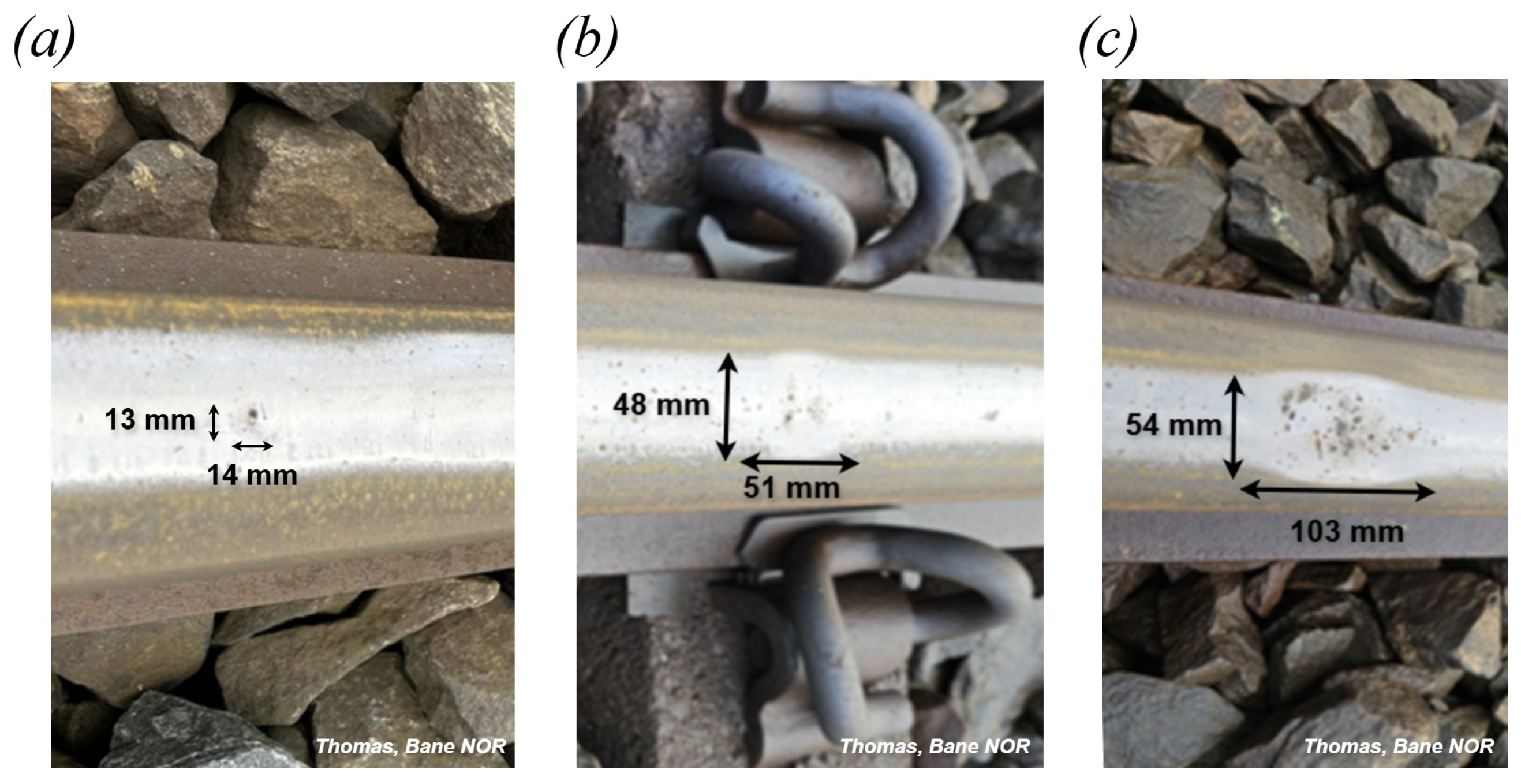
Figure 1. Classified rail squats. Photography: Thomas Vatn Bjørge/Bane NOR, Vestfoldbanen, Norway: (a) light; (b) moderate; (c) severe.
Infrastructures 10 00313 g001
Figure 2. Methods: (a) train model in side view and track model in rear view; (b) The squat simulation curves and 3D view for one example case S25; (c) The installation locations of the accelerometers, which serve as monitoring points, are labeled in side, top, front and 3D views. (d) The analysis pipeline for using vertical vibration response for rail squat detection.
Infrastructures 10 00313 g002
Figure 3. Optimal accelerometer placement analysis results, highlighting the lowest values with red boxes and the squat center with a dotted line: (a) P corr heat map in the time domain for wheel sets under various train speeds (20 km/h, 80 km/h, 160 km/h); (b) The first wheel set displacement for a total of 25 squat cases (S1–S25); (c) P corr heat map, accelerations, and response spectra of the first wheel set; (d) for the first bogie; (e) for the car body.
Infrastructures 10 00313 g003
Figure 4. Correlation sensitivity analysis between squat features and acceleration for various train speeds; (a) squat length for the optimal locations of wheel set, bogie, and car body; (b) squat depth.
Infrastructures 10 00313 g004
Figure 5. Measured acceleration response for five squat length cases (S5–S25: 10–50 mm) under train speeds (20, 40, 60, 80, and 160 km/h). The dotted line indicates the longitudinal center of the squats.
Infrastructures 10 00313 g005
Figure 6. Acceleration analysis for five squat length cases (S5–S25: 10–50 mm) under train speeds (20, 40, 60, 80, and 160 km/h): (a) Frequency-domain response; (b) Time-domain extrema. ( M 1 : global maximum; m 1 : global minimum; M 2 : local maximum); (c) Phase delay characteristics ( M 1 , m 1 , M 2 ).
Infrastructures 10 00313 g006
Figure 7. Mechanism in the longitudinal direction.
Infrastructures 10 00313 g007
Figure 8. Mechanism in the longitudinal direction when the squat length is increased. The solid and dotted lines show the vertical acceleration after and before the increase.
Infrastructures 10 00313 g008
Figure 9. Mechanism in the vertical and longitudinal directions.
Infrastructures 10 00313 g009
Figure 10. Mechanism in the longitudinal direction when the squat depth is increased. The solid and dotted lines show the vertical acceleration after and before the increase.
Infrastructures 10 00313 g010
Figure 11. Mechanism in the longitudinal direction when the train speed is increased. The solid and dotted lines show the vertical acceleration after and before the increase.
Infrastructures 10 00313 g011
Figure 12. Comparison of number of samples per mm in the longitudinal direction for 20 kHz vs. 100 kHz when train speed is 160 km/h. The dotted line indicates the longitudinal center of the squats.
Infrastructures 10 00313 g012
Table 1. Parameters of the train-track model.
ParameterValuesUnits
car body mass36,467kg
Bogie mass5192kg
wheel set mass1599kg
Primary suspension, vertical springs 7.0 × 10 7 N/m
Primary suspension, vertical dampers 6.0 × 10 4 Ns/m
Secondary suspension, vertical springs 5.0 × 10 6 N/m
Secondary suspension, vertical dampers 4.0 × 10 4 Ns/m
Secondary suspension, air suspensions 8.5 × 10 4 Ns/m
Secondary suspension, bump stops 5.0 × 10 6 N/m
car body-bogie mass center distance9.5m
Bogie-wheel set mass center distance1.35m
wheel set radius0.45m
Wagon coupling, longitudinal springs 3.4 × 10 6 N/m
Wagon coupling, longitudinal dampers 4.0 × 10 4 Ns/m
Track-ground coupling, vertical springs 1.5 × 10 5 N/m
Track-ground coupling, vertical damping 9.8 × 10 5 Ns/m
Track-ground coupling, lateral springs 4.0 × 10 7 N/m
Track-ground coupling, lateral damping 9.1 × 10 5 Ns/m
wheel–rail modelwr_coupl_pe4;
fasim lookup table
Eigen frequency f 1 (vertical bending motion mode)9.9Hz
Eigen frequency f 2 (lateral bending motion mode)9.8Hz
Eigen frequency f 3 (cross-sectional shear motion mode)12.2Hz
Eigen frequency f 4 (longitudinal bending motion mode)12.7Hz
Table 2. Correlation levels between six indicators and squat length: O = Optimal (linear correlation), △ = Conditional (non-linear correlation), × = Avoid (no significant correlation).
Train Speed (km/h) M 1 , acc m 1 , acc M 2 , acc M 1 , pd m 1 , pd M 2 , pd
20OOO×
40OOO×
60OOOO×
80OOOOO×
100OOOOO×
120OOOO×
140OOOO×
160OOOO×
Table 3. Correlation levels between six indicators and squat depth: O = Optimal (linear correlation), △ = Conditional (non-linear correlation), × = Avoid (no significant correlation).
Train Speed (km/h) M 1 , acc m 1 , acc M 2 , acc M 1 , pd m 1 , pd M 2 , pd
20×××
40×××
60×O×
80×O×
100×O×
120×O×
140×O×
160×O×
Table 4. Estimated squat center position ( x 0 ^ ) and relative accuracy ( Δ x 0 ) for five squat lengths 10–50 mm (cases S5–S25) at train speeds varying from 20 to 160 km/h.
Squat Length (mm) (Case)
x 0 ^   ( mm )   ( Δ x 0 ) 10
(S5)
20
(S10)
30
(S15)
40
(S20)
50
(S25)
Train Speed (km/h)
200.00 (100.00%)0.84 (95.83%)−0.56 (98.15%)−1.11 (97.23%)−1.11 (97.78%)
400.61 (93.90%)0.78 (96.13%)0.78 (97.40%)1.45 (96.39%)2.00 (96.00%)
600.92 (90.85%)0.84 (95.83%)1.08 (96.40%)1.58 (96.05%)1.83 (96.34%)
800.45 (95.55%)0.78 (96.13%)0.56 (98.15%)1.34 (96.66%)1.34 (97.33%)
1000.28 (97.25%)0.14 (99.33%)0.42 (98.60%)0.84 (97.91%)1.12 (97.77%)
120−0.17 (98.30%)0.00 (100.00%)−0.17 (99.45%)0.50 (98.75%)0.66 (98.67%)
140−0.31 (96.95%)−0.31 (98.48%)−0.31 (98.97%)0.08 (99.79%)0.28 (99.44%)
160−0.45 (97.78%)−0.23 (98.88%)0.44 (98.52%)−0.23 (99.44%)0.23 (99.55%)
Table 5. Estimated squat length ( x 2 a ^ ) and relative accuracy ( Δ x 2 a ) for five squat lengths 10–50 mm (cases S5–S25) at train speeds ranging from 20 to 160 km/h.
Squat Length (mm) (Case)
x 2 a ^   ( mm )   ( Δ x 2 a ) 10
(S5)
20
(S10)
30
(S15)
40
(S20)
50
(S25)
Train Speed (km/h)
207.78 (77.80%)16.11 (80.55%)21.11 (70.37%)27.78 (69.45%)36.66 (73.32%)
408.78 (87.80%)16.67 (83.35%)24.44 (81.47%)33.11 (82.78%)40.22 (80.44%)
608.83 (88.30%)16.67 (83.35%)24.50 (81.67%)33.50 (83.75%)41.00 (82.00%)
808.89 (88.90%)16.67 (83.35%)24.67 (82.23%)33.33 (83.33%)41.33 (82.66%)
1008.89 (88.90%)16.39 (81.95%)24.72 (82.40%)33.89 (84.73%)41.11 (82.22%)
1209.00 (90.00%)16.66 (83.30%)24.33 (81.10%)33.66 (84.15%)41.33 (82.66%)
1408.95 (89.50%)16.73 (83.65%)24.50 (81.67%)33.05 (82.63%)41.22 (82.44%)
1608.89 (88.90%)17.33 (86.65%)26.67 (88.90%)33.33 (83.33%)41.33 (82.66%)
Table 6. List of accelerometers for railway track condition monitoring with key parameters.
Sensor TypeMeasurement Range
(g)
Sensitivity
(mV/g)
Resolution
(g)
Sample Frequency
(kHz)
References
PCB 354C02±50010 mV/g0.0005 g20 kHz [37]
VIS 311A±50100 mV/g0.00035 g20 kHz [38]
J1 3510±25020 mV/g0.005 g20 kHz [39]
CARS CS01AC±20025 mV/g0.0005 g5 kHz [40,41]
Disclaimer/Publisher’s Note: The statements, opinions and data contained in all publications are solely those of the individual author(s) and contributor(s) and not of MDPI and/or the editor(s). MDPI and/or the editor(s) disclaim responsibility for any injury to people or property resulting from any ideas, methods, instructions or products referred to in the content.