Machine Learning Synthesis of Fire-Following-Earthquake Fragility Surfaces for Steel Moment-Resisting Frames

Abstract

This paper presents a probabilistic methodology for generating fragility surfaces for low- to mid-rise steel moment-resisting frames (MRFs) under fire-following-earthquake (FFE). The framework integrates nonlinear dynamic seismic analysis, residual deformation transfer, and temperature-dependent fire simulations within a Monte Carlo environment, while explicitly accounting for uncertainties in structural properties, ground motions, and fire simulation. A fiber-based modeling strategy is employed, combining temperature-sensitive steel materials with fatigue and fracture wrappers to capture cyclic deterioration and abrupt failure. This formulation yields earthquake-only and fire-only fragility curves along the surface boundaries, while interior points quantify the joint fragility response under sequential hazards. The methodology is benchmarked against a machine learning (ML) synthesis framework originally developed for earthquake–tsunami applications and extended here to FFE. Numerical results for a three-story steel MRF show excellent agreement (R² > 0.95, RMSE < 0.02) between simulated and ML-generated surfaces, demonstrating both the efficiency and hazard-neutral adaptability of the ML framework for multi-hazard resilience assessment.

1. Introduction

Historic events have shown that post-earthquake fires can be as devastating as the seismic shaking itself. The 1906 San Francisco earthquake triggered over 50 fires, with approximately 80% of the city’s destruction attributed to these fires rather than the earthquake itself [1,2]. Similarly, the 1923 Great Kantō earthquake in Japan resulted in widespread conflagrations responsible for nearly 78% of the total damage and over 140,000 fatalities [1,3,4,5]. More recent disasters, such as the 1995 Kobe earthquake in Japan, which caused numerous urban fires [6], and the 2011 Christchurch earthquake in New Zealand, where fire outbreaks compounded seismic damage [7], underscore that fire-following-earthquake remains a persistent threat in modern cities. These events highlight the significant risk posed by fire-following-earthquake (FFE) scenarios, particularly in dense urban environments where earthquake-induced damage compromises both structural integrity and firefighting capabilities [8,9,10].

Earthquakes often rupture gas lines, damage electrical systems, and disable fire suppression mechanisms, creating conditions highly conducive to fire outbreaks [9]. Additionally, compromised water supply and obstructed transportation routes hinder emergency response efforts [11,12]. Despite this well-documented cascading hazard, current design practices typically address seismic and fire risks independently. Building codes and standards such as ASCE 7-22 (2022) [13] and Eurocode 2 and Eurocode 8, 2nd Generation Drafts [14,15,16], prescribe separate criteria for seismic and fire loading, failing to account for their sequential or combined effects. Performance-based design (PBD) frameworks have advanced single-hazard risk assessment, particularly in seismic engineering through methodologies like FEMA P-58 (2012) [17] and FEMA P-695 (2009) [18]. However, these frameworks do not explicitly address cascading hazards such as FFE. While multi-hazard guidance exists for earthquake–tsunami scenarios, i.e., FEMA P-646 (2019) [19], there is a critical gap regarding sequential earthquake-fire risks [20,21]. This omission leaves structures potentially vulnerable to compounded damage when fire follows seismic events.

Steel moment-resisting frames (MRFs), widely used in seismic regions due to their ductility and energy dissipation capacity, face unique vulnerabilities under FFE conditions [22,23,24,25]. Research has shown that seismic damage degrades fire resistance by displacing fireproofing materials and compromising structural elements [26]. Full-scale experiments, such as those conducted at UC San Diego, have demonstrated how earthquake-induced residual drifts and breached compartmentation exacerbate fire spread and structural degradation [9,27,28,29]. To address these challenges, probabilistic methods and fragility analysis are increasingly being adopted for multi-hazard scenarios [30,31]. Fragility functions, which quantify the probability of exceeding damage states (DSs) given hazard intensities, are well-established in earthquake engineering [32,33]. Recent efforts have extended this concept to fire [34,35,36], and preliminary frameworks for FFE fragility modeling have emerged [21,37,38]. These studies emphasize the necessity of capturing uncertainties related to both hazards and the progressive degradation of structural capacity.

In dense urban areas surrounded by forests—particularly in dry climates such as Los Angeles—the ignition point of a mass fire may originate within the town itself rather than in the wildland perimeter [10,39]. Integrating performance-based earthquake and fire engineering into a unified FFE fragility framework provides a pathway to more resilient structural design [37]. By quantifying the probability of collapse or critical DSs under cascading hazards, such models can inform targeted risk mitigation strategies and guide updates to building codes [38]. Advancing this field is essential for safeguarding communities in seismically active regions where the threat of post-earthquake fires remains a persistent and under-addressed risk.

This paper introduces and validates a comprehensive methodology for generating fragility surfaces of steel moment-resisting frames under fire-following-earthquake. The framework integrates nonlinear dynamic earthquake analysis, residual deformation transfer, and probabilistic fire simulation within a Monte Carlo environment, while explicitly accounting for structural and hazard-related uncertainties. A fiber-based modeling strategy is employed to capture temperature-dependent degradation, cyclic deterioration, and ultimate fracture, ensuring realistic collapse representation. The methodology is further examined against a machine learning-based synthesis approach originally developed for earthquake–tsunami sequences, adapted here to earthquake–fire hazards. Through a case study on a three-story steel MRF, the study demonstrates how the proposed framework can be used to derive multi-dimensional fragility surfaces, evaluate the agreement between simulation- and ML-generated models, and provide probabilistically consistent insights into structural performance under cascading hazards.

2. Methodology to Generate Integrated FFE Fragility Surface

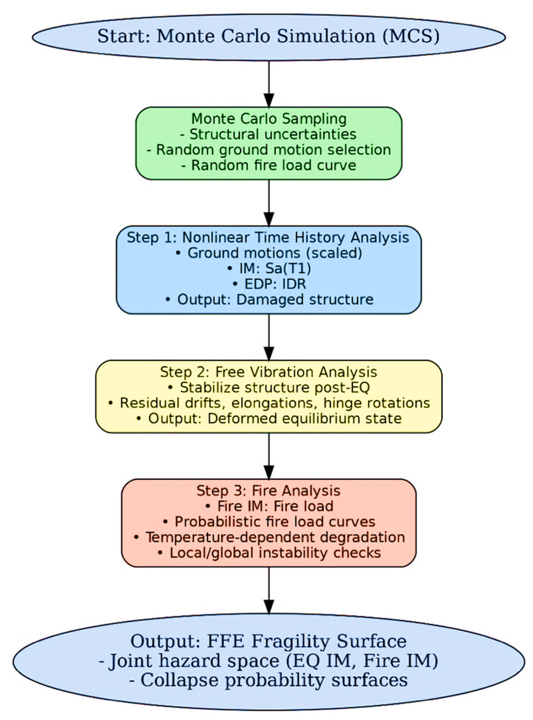
The proposed methodology follows a three-step sequential analysis framework to capture the cascading effects of earthquake and fire on steel MRFs. The framework integrates nonlinear dynamic seismic response, residual deformation transfer, and subsequent fire exposure into a robust procedure for FFE fragility surface generation. Each successive simulation is performed within a Monte Carlo Simulation (MCS) environment, enabling uncertainty quantification and probabilistic estimation of collapse prevention or failure thresholds. The sequential procedure for generating FFE fragility surfaces is summarized in the flowchart shown in Figure 1.

The first stage consists of nonlinear time history analysis under earthquake excitation, with the structural system initialized at ambient temperature equal to the surrounding environment. The finite element model (described in Section 3) is subjected to a suite of ground motions selected from predefined bins, with scaling applied using the point-scaling method. Spectral acceleration at the fundamental period, Sa(T₁), is adopted as the earthquake intensity measure (IM), following common practice in multi-hazard fragility modeling [40,41]. For each ground motion, the structural model is sampled stochastically to reflect uncertainties in material properties, geometric imperfections, and damping characteristics. The engineering demand parameter (EDP) in this phase is the inter-story drift ratio (IDR) [40], with complete or collapse-prevention DSs adopted from HAZUS (2020) [42] thresholds. The outcome of this phase is a seismically damaged structure, including residual drifts and local deterioration, which is then carried forward into the next step. Similar to the hybrid OpenSees [43,44] modeling approach by Saed et al. (2025) [45], the model accounts for cyclic degradation mechanisms to ensure realistic representation of seismic damage.

To capture post-seismic permanent displacements, a free vibration analysis is performed immediately after the time history analysis under each ground motion record. This step allows the system to stabilize dynamically, converging toward its deformed equilibrium state [46,47]. The resulting configuration incorporates residual inter-story drifts, beam elongations, and potential plastic hinge rotations, which represent the initial conditions for the subsequent fire analysis. This procedure is consistent with sequential frameworks used in prior studies of post-earthquake fire (PEF) modeling (e.g., Saed et al. (2025) [45]), where the deformed shape of the system directly influences thermal expansion demands, load redistribution, and local instabilities during fire.

The seismically damaged and deformed structural model is then subjected to a rising temperature profile defined through probabilistic fire load curves. While various fire IMs (e.g., duration, maximum temperature, area under temperature–time curve) exist in the literature [35,48], this study adopts fire load as the fire IM, as it provides a more direct quantification of thermal severity [49]. The thermal analysis applies time–temperature relationships to heated members, with fire-induced degradation in material stiffness and strength modeled using temperature-dependent constitutive laws [50,51,52]. Following practices demonstrated in recent OpenSees hybrid modeling efforts (e.g., Jiang et al. (2015) [51]), local stability is evaluated by tracking the reduction in beam and column strength to 80% of their maximum capacity [45], while global mechanisms are assessed through IDR thresholds similar to those defined in Step 1 [53]. Together, these limit states capture both localized instability (loss of load-carrying capacity in critical members) and global collapse-type responses.

The integrated procedure is executed probabilistically through MCS, where each simulation involves random generation of structural parameters through uncertainty sampling, selection of a ground motion from the earthquake bin scaled appropriately, nonlinear time history analysis under earthquake loading (Step 1), free vibration analysis to transfer residual deformation (Step 2), and sequential fire analysis under probabilistic fire loads (Step 3).

The binary outcome of each run (failure or survival at a given earthquake–fire IM pair) is accumulated across all simulations to calculate the conditional probability of exceeding specified limit states. These raw results are converted into multi-dimensional and multi-hazard FFE fragility surfaces, representing the joint hazard space of earthquake intensity and fire severity. The raw failure probability points can be fitted by a closed-form probabilistic surface function, originally adapted from Harati and van de Lindt (2024a) [46], which estimates the conditional exceedance probability for any earthquake–fire IM pair. The surface is expressed as:

$$P\left({IM}_{EQ},{IM}_{Fire}\right)={\displaystyle \frac{E{(\frac{{IM}_{EQ}}{C_1}+\frac{{IM}_{Fire}}{C_2}+\alpha \left(\frac{{IM}_{EQ}}{C_1}\right)\left(\frac{{IM}_{Fire}}{C_2}\right))}^n}{({\left(\frac{{IM}_{EQ}}{C_1}+\frac{{IM}_{Fire}}{C_2}+\alpha \left(\frac{{IM}_{EQ}}{C_1}\right)\left(\frac{{IM}_{Fire}}{C_2}\right)\right)}^n+1)}}$$

(1)

where ${IM}_{EQ}$ and ${IM}_{Fire}$ denote the IMs for the earthquake (e.g., spectral acceleration at the fundamental period) and fire (e.g., equivalent temperature or fire load parameter), respectively. The parameters E, C₁, C₂, α, and n are fitting constants that control the scale, steepness, and interaction between the two hazards. Once the successive simulation model produces exceedance probabilities over a discretized (${IM}_{EQ},{IM}_{Fire}$) grid, a nonlinear regression algorithm (e.g., scipy.optimize.curve_fit) is used to calibrate the five parameters (see Harati and van de Lindt (2024a) [46] for details). This closed-form representation allows compact storage of fragility surfaces while providing sufficient flexibility to capture nonlinear damage accumulation and hazard interaction effects characteristic of earthquake–fire sequences.

3. Structural Modeling

The methodology developed in this study for structural modeling is designed for low- to mid-rise steel moment resisting frames subjected to PEF scenarios. While concentrated plastic hinge models (e.g., modified IMK hinges) [54,55] are often considered superior for collapse simulations due to their ability to capture deterioration of stiffness and strength [56,57], the present framework adopts a fiber-based approach. This choice is essential because it allows the temperature–time history to be directly embedded in the element formulation [45,51], particularly in the third phase of analysis where fire governs structural performance. 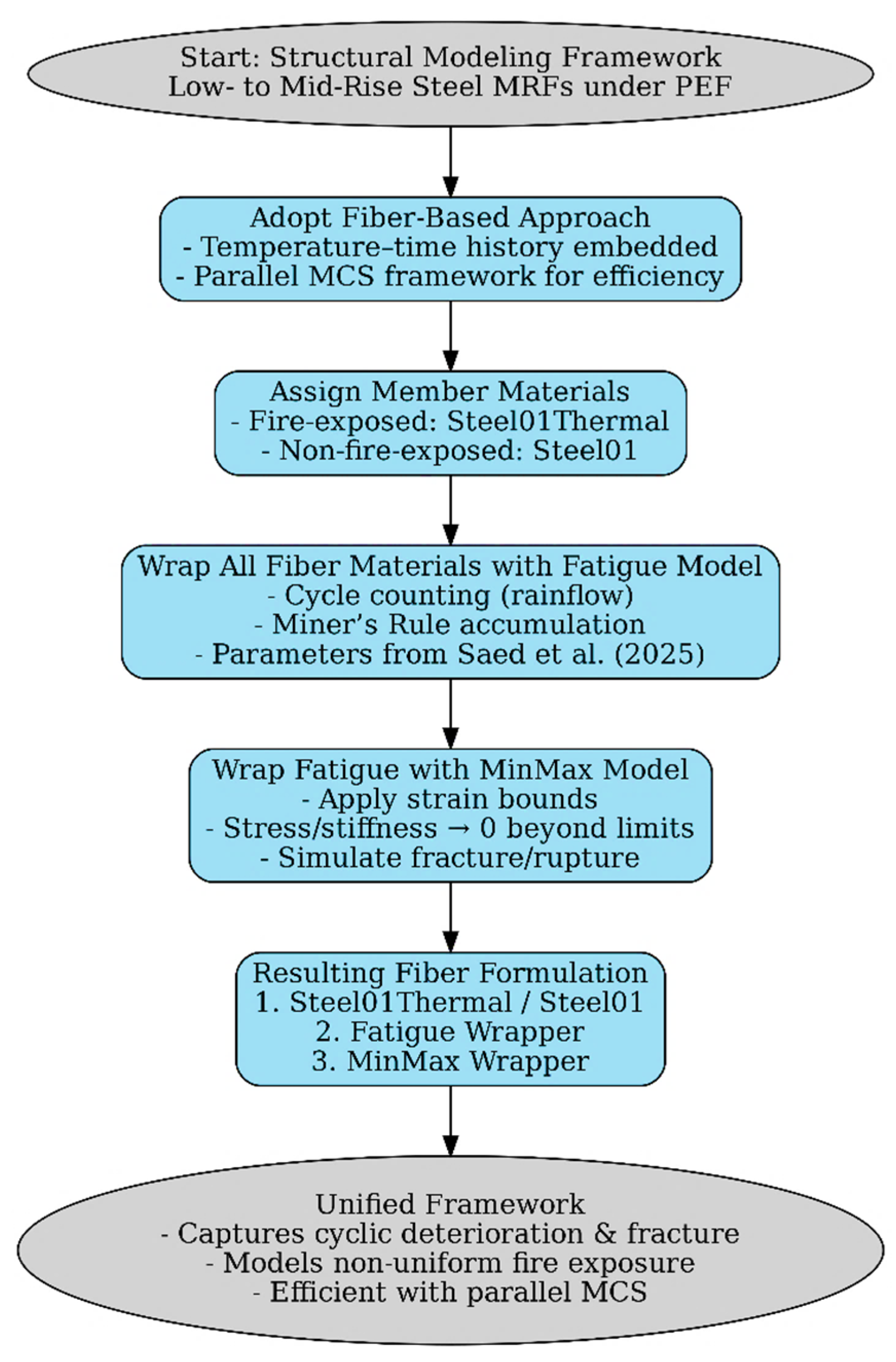Computational demands, a common limitation of fiber approaches, are addressed by implementing the simulations within a multi-distributed MCS framework with parallel processing [58]. The stepwise framework for structural modeling is summarized in Figure 2, which illustrates the fiber-based methodology developed for steel MRFs under post-earthquake fire conditions.

In this approach, structural members are modeled using displacement-based beam-column elements with fiber sections. For elements directly exposed to fire, the Steel01Thermal material is assigned. This thermal extension of the widely used Steel01 model incorporates temperature sensitivity by requiring inputs of yield strength (F_y), elastic modulus (E₀), strain-hardening ratio (b), and optional isotropic hardening parameters (a₁–a₄). For non-fire-exposed members, the regular Steel01 formulation is used, reducing computational cost while preserving accuracy. By combining thermal and non-thermal fibers, the model captures the non-uniform thermal exposure expected in realistic fire scenarios.

To address cumulative cyclic deterioration, which is not inherently captured in fiber sections, each fiber section material is wrapped with the Fatigue material in OpenSees [43,44,59]. This model employs a modified rainflow cycle counting algorithm with Miner’s Rule to track damage accumulation until fatigue life is exhausted [60]. Key parameters include E₀ (strain at which one cycle induces failure) and m (slope of the Coffin–Manson curve). As demonstrated by Saed et al. (2025) [45], calibrated parameter values effectively replicate experimentally observed deterioration under combined seismic and thermal demands. This allows the fiber-based model to emulate the hysteretic degradation typically represented in modified IMK hinges [55], where low-cycle fatigue effects are embedded through experimental calibration. The fatigue and MinMax wrapper parameters were selected based on calibration to low-cycle fatigue test data and prior numerical studies [45,60], ensuring consistency with experimentally observed deterioration and fracture behavior in steel MRF components. The parameter values were verified to yield realistic hysteretic degradation and ultimate strain limits consistent with available experimental benchmarks.

To further control ultimate failure, the fatigue-wrapped material is then encapsulated with the MinMax material in OpenSees. The MinMax model applies lower and upper strain bounds to the parent material response [61]. When the fiber strain falls outside these thresholds, both stress and tangent stiffness drop to zero, simulating fracture or rupture at large elongations. In this layered configuration, the fatigue model governs cyclic deterioration, while MinMax governs final fracture behavior, thereby ensuring a comprehensive representation of material failure mechanisms.

The resulting fiber formulation can be described as a three-layered nesting scheme: (1) Steel01Thermal for temperature-sensitive stress–strain response in fire-exposed members and Steel01 for non-fire-exposed members; (2) a Fatigue wrapper applied to all fibers to capture low-cycle fatigue accumulation; and (3) a MinMax wrapper applied to all fibers to enforce large-strain fracture limits. While only fire-exposed elements incorporate temperature-dependent behavior through Steel01Thermal, every fiber section in the model—whether thermal or non-thermal—is wrapped with Fatigue and MinMax to ensure consistent representation of cyclic deterioration and ultimate fracture across the entire frame. This strategy maintains computational efficiency while providing a unified framework for simulating progressive collapse (i.e., a potential scenario in this fragility modeling) under combined seismic and fire demands. Overall, this methodology balances the fidelity of concentrated hinge models with the necessity of temperature-dependent fiber modeling in PEF studies. By embedding thermal degradation, cyclic fatigue, and fracture into a single fiber-based scheme, the framework provides a robust and computationally feasible platform for collapse and fragility assessment. The approach ensures that both strength and stiffness deterioration are realistically captured, while parallelized MCS implementation [46] makes the methodology suitable for large-scale resilience evaluations of steel MRFs under sequential earthquake–fire loading.

Earthquake and Fire Loadings

Gravity loads are modeled using probabilistic distributions to propagate uncertainties, which will be detailed in the following section (Section 4). For the seismic hazard, far-field ground motion records from FEMA P-695 (2009) [18] are employed as input. These records are scaled using the point scaling method across different seismic intensity levels, consistent with the multiple stripe analysis (MSA) framework [62] implemented within the proposed MCS procedure. 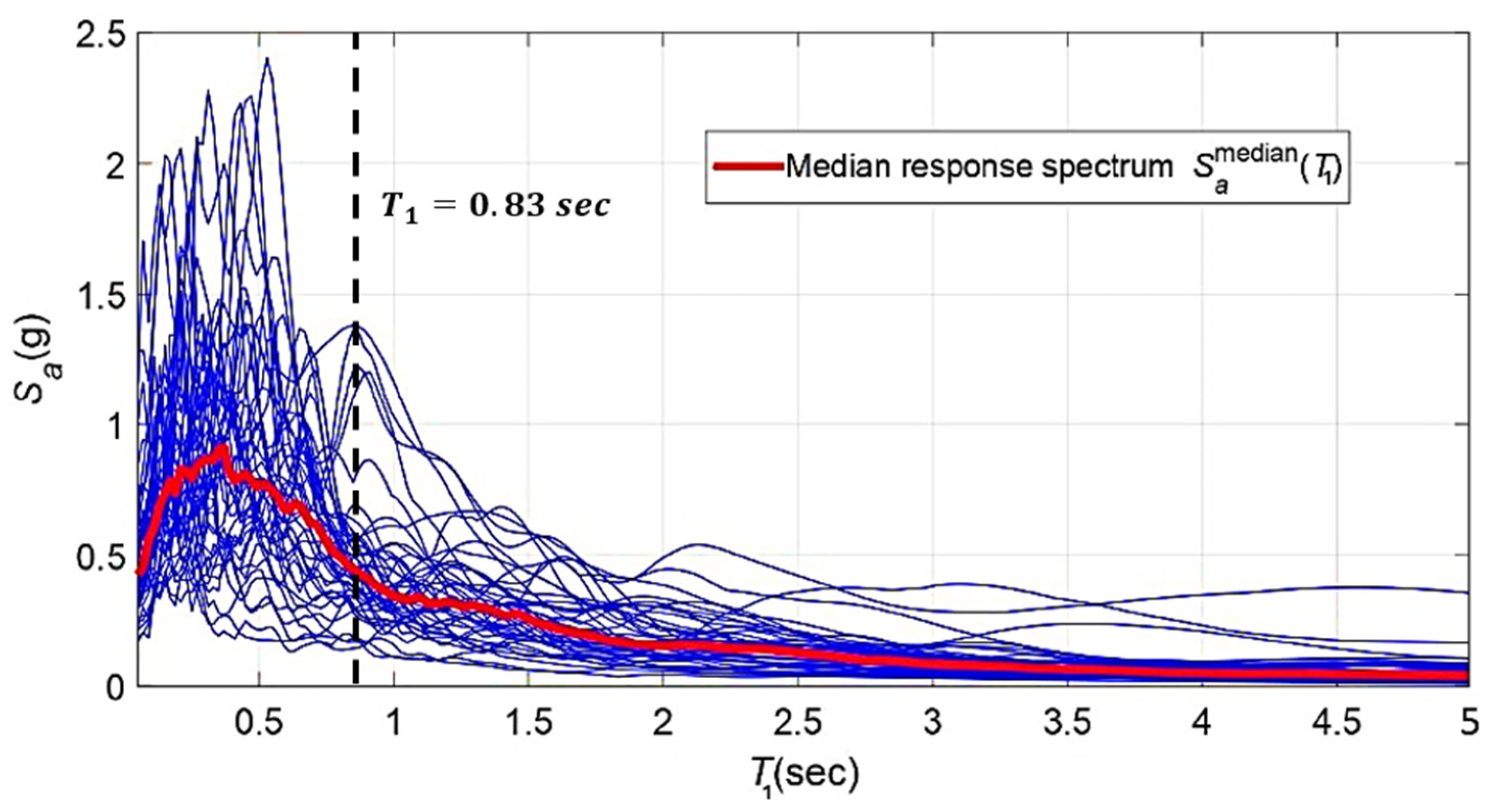This scaling approach aligns with common practices in MSA and incremental dynamic analysis (IDA) [63], ensuring that the treatment of earthquake loading is consistent with methodologies typically applied when seismic hazard is considered in isolation (e.g., see [33]). The seismic input used in this study is illustrated in Figure 3, which presents the response spectra of the selected FEMA P-695 far-field ground motion records. Each line corresponds to the spectral acceleration (Sa) of an individual record, while the thicker line denotes the median response spectrum across all records. The figure highlights the variability in spectral demand at short periods and the convergence toward lower values at longer periods. Using the median spectrum ensures that the seismic hazard representation is consistent with standard practice for multiple-stripe or incremental dynamic analysis, while also capturing the dispersion of individual records needed for probabilistic assessment.

For the fire hazard, prior research has shown that the worst-case scenario occurs when fire engulfs the entire first story of the structure [21,23,45,64,65]. Accordingly, only the beams and columns of the first story are modeled with thermally sensitive fiber sections. To realistically simulate fire-induced deformations, equal degrees of freedom are disabled at the first floor, thereby permitting independent thermal elongation of members, especially beams, and allowing the model to capture violations of the rigid diaphragm assumption expected under severe fire exposure [45].

The model of the examined frame (discussed later) is built in OpenSees [43] using the dispBeamColumnThermal elements with Steel01Thermal material. The members are uniformly heated to more than 550 °C approximately, reaching a state of instability under the ISO-834 standard fire curve [15]. The temperature defined in this standard curve is applied as a boundary condition, with the expression later modified to enable uncertainty propagation:

T = 20 + 345 log(8t + 1)

(2)

where t represents time in minutes. This choice reflects both the embedded functionality of Steel01Thermal and the widespread adoption of the ISO-834 curve in structural fire analysis [66]. While other time–temperature curves exist in the literature, the use of ISO-834 ensures direct compatibility with the OpenSees thermal module and facilitates a consistent representation of material degradation under elevated temperatures [67].

The maximum gas temperature in the compartment fire model was expressed as a function of both the fire load density and the ventilation opening factor, consistent with Eurocode parametric fire formulations [68,69]. In this study, a simplified surrogate relation was adopted to approximate the peak temperature:

T_max = 1325 (1 − e^−0.01qO)

(3)

where q denotes the fire load density (MJ/m²) and O is the opening factor. This expression reflects the asymptotic behavior of Eurocode parametric curves, which saturate toward approximately 1325 °C while accounting for increases in fire severity with greater combustible energy and ventilation. The coefficient (0.01) serves as a calibration parameter to align the surrogate with Annex A of EN 1991-1-2 [16] over the practical range of q and O. While the canonical Eurocode model provides a time-temperature trajectory, the above formulation offers a computationally efficient representation of the expected peak, suitable for Monte Carlo-based fragility analyses where repeated evaluations are required.

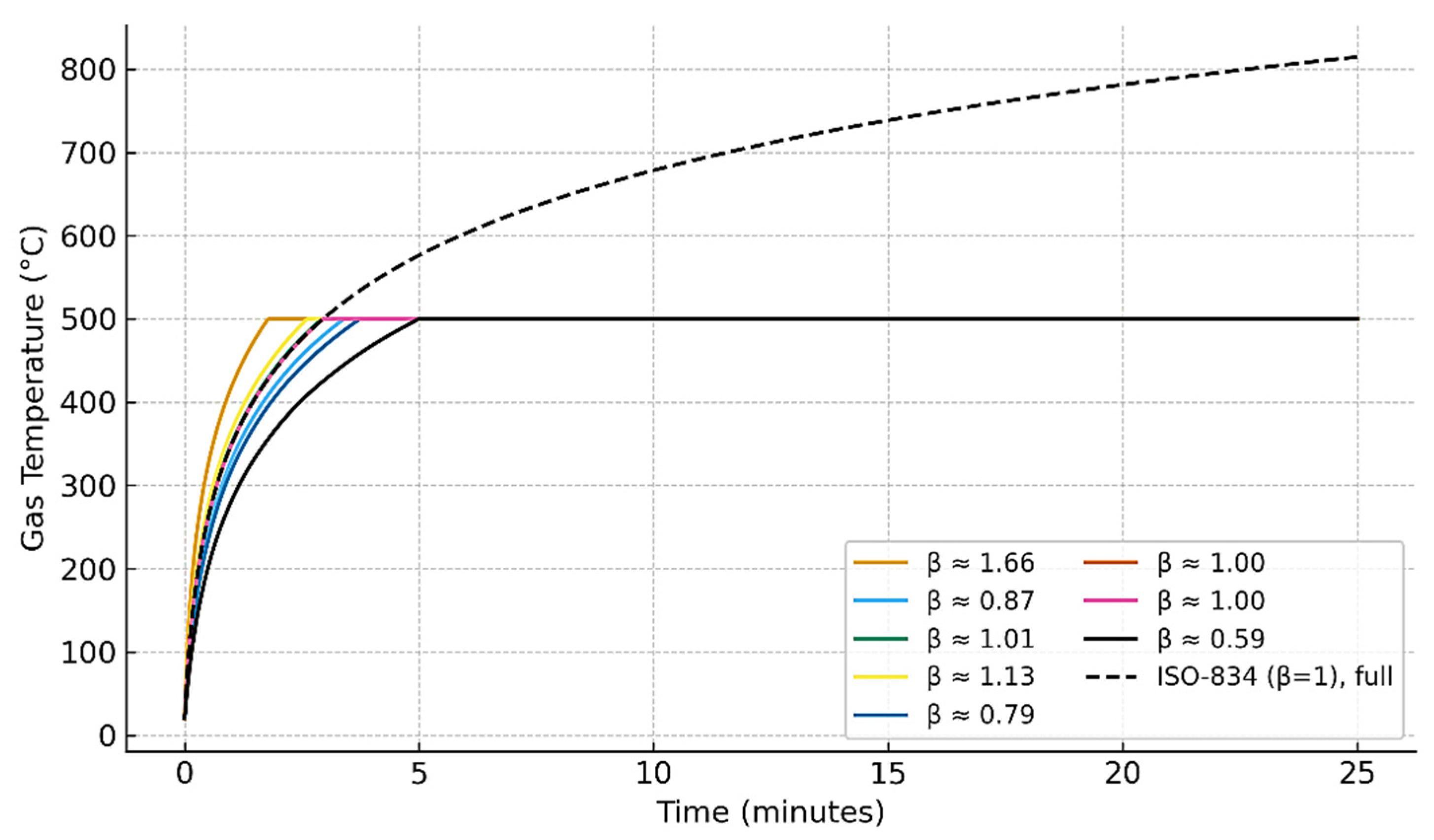
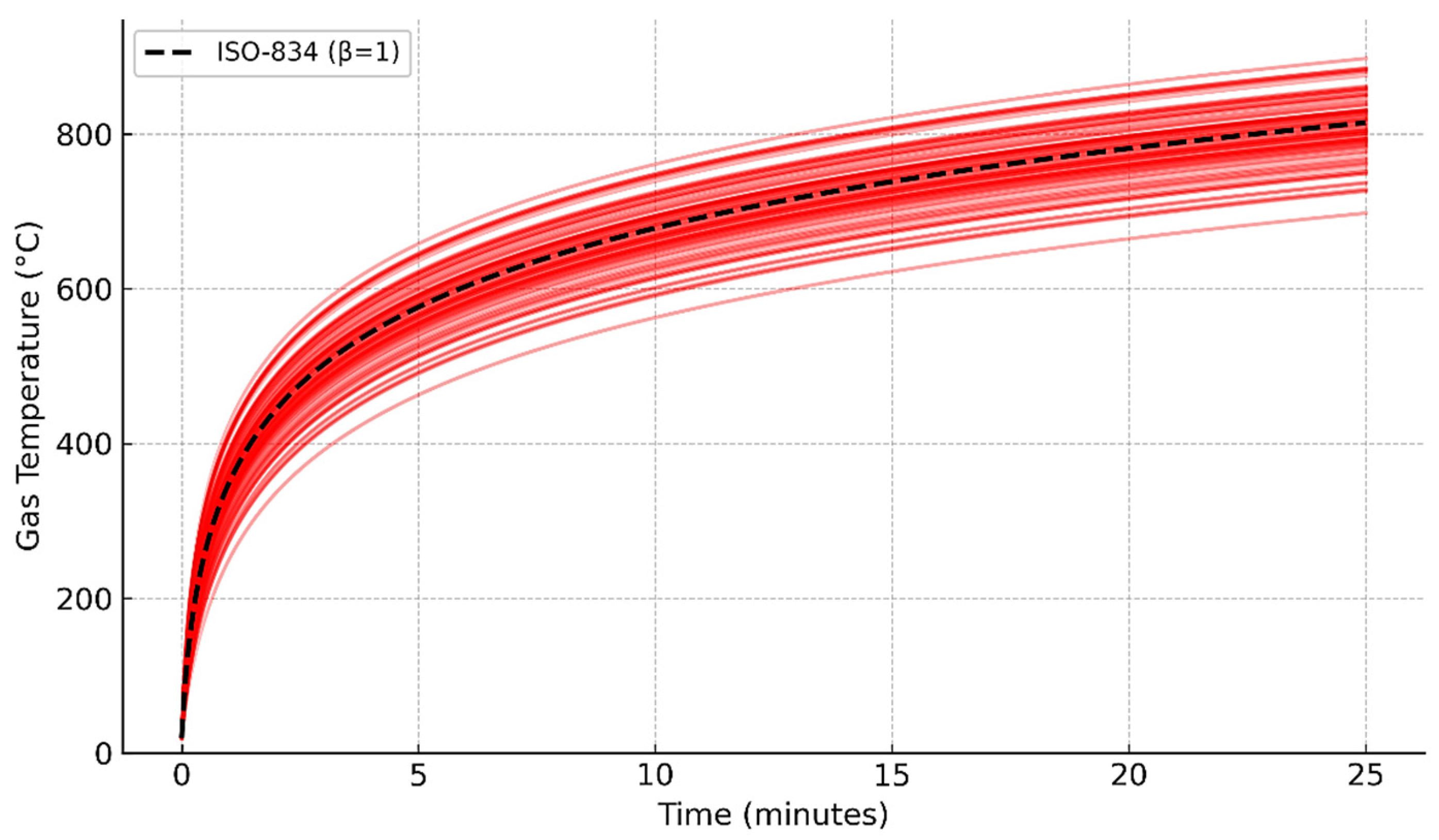
The procedure begins by selecting a fire load value (q), from which the corresponding maximum temperature (T_max) is obtained using Equation (3). A randomly distributed fire duration (t) is then sampled (as discussed later) to ensure that the ISO-834 curve, expressed in Equation (2), reaches the same T_max. The variability of the resulting heating trajectories is illustrated in Figure 4, where the ISO-834 formulation is modified by introducing a lognormally distributed β factor multiplied to fire duration, t. This parameter governs the growth rate of the fire curve while preserving its asymptotic behavior. As shown in Figure 4, different realizations of β produce distinct heating curves within the first 25 min, all truncated at 500 °C. The reference ISO-834 curve (β = 1) is also plotted for comparison, demonstrating how the probabilistic treatment captures uncertainty in fire development while remaining consistent with the standardized model.

Through this combined loading protocol, the sequential effects of earthquake and fire are represented in a probabilistically consistent manner, ensuring that the interaction between seismic damage and subsequent thermal degradation is explicitly captured. The modeling strategy emphasizes the first-story members, which act as the critical components governing collapse potential, since both experimental and analytical studies have shown that failure is typically initiated at the base level where gravity demands are highest and fire exposure is most severe [23,45]. By embedding stochastic variability in both seismic input and fire development, the framework enables the generation of fragility functions that reflect not only mean performance but also the uncertainty associated with hazard intensity, damage accumulation, and structural deterioration.

4. Uncertainty Quantification

Uncertainty in the structural model is incorporated to capture variability in key parameters influencing dynamic and thermal response. Following established reliability studies [70,71], both dead load and seismic mass were modeled as lognormally distributed with a mean of 1.05 multiplied by the computed value and a coefficient of variation (COV) of 0.10. For steel structures, the dominant source of material property uncertainty arises from variability in the yield strength (f_y) of steel fibers [70,71,72]. In this study, f_y was modeled as a lognormal random variable with a mean of 60 ksi (415 MPa) and a COV of 10% [71].

For the earthquake phase of the successive simulation, structural and input uncertainties were explicitly incorporated to capture the variability in seismic demand and response. The damping ratio was modeled as a lognormal variable with a mean of 0.065 and a COV of 0.60, consistent with the large scatter observed in experimental studies [71]. In addition, uncertainty in the seismic input motions was addressed by employing a bin of 44 far-field ground motion records recommended in FEMA P-695 [18]. These records were scaled across different intensity levels and used as input for the first phase of the simulation framework, thereby ensuring that both record-to-record variability and modeling uncertainties were propagated into the fragility analysis [73]. These probabilistic representations allow uncertainty in structural capacity and energy dissipation to be propagated consistently through the MCS procedures, ensuring that fragility estimates reflect both hazard and modeling variability. The Monte Carlo simulation framework was executed over thousands to millions of realizations, depending on the discretization of the joint intensity measure (IM) grid. Similar to the procedure established by Harati and van de Lindt (2025) [41], a pilot convergence analysis was first performed using $K_{initial}=10$ samples to estimate the variance of failure probability at each IM pair. The required sample size was iteratively refined using $n_r=(Z^2{\sigma }^2/E_r^2)$, targeting a 95% confidence level and an average error below 1%. The mean collapse probability stabilized at less than 1% variation across successive iterations, confirming convergence and statistical reliability of the final fragility surface. All uncertainty variables—including structural, seismic, and fire-related parameters—are jointly sampled in each Monte Carlo realization. To maintain statistical consistency across the sequential earthquake–fire phases, the random variables are generated simultaneously using Latin Hypercube Sampling (LHS), ensuring appropriate coverage of the joint parameter space and correlation among variables within each simulation.

Uncertainty in structural fire performance arises not only from variations in material properties and boundary conditions but also from the stochastic nature of fire development itself [74,75]. The thermal demand imposed on structural members depends on numerous uncertain parameters, including fire load density, compartment geometry, and ventilation conditions. To reflect this variability, a probabilistic framework was adopted in this study, where uncertainty in the fire curves is introduced through a lognormal distribution applied to the fire growth factor (β) [74]. The rationale for selecting a lognormal distribution is twofold. First, fire load and ventilation-related variables are inherently positive, making the lognormal a natural choice for representing skewed, non-negative random variables. Second, prior studies have shown that lognormal-type distributions provide a realistic statistical representation of fire load variability observed in experimental and field data [76,77]. By sampling β from a lognormal distribution centered around unity, the baseline ISO-834 curve can be stochastically perturbed, producing a family of fire curves that reflect uncertainty in the heating rate while preserving the standardized asymptotic shape.

In practice, the ISO-834 expression, T = 20 + 345 log(8βt + 1), was modified by introducing the random multiplier β into the time-scaling term. For each Monte Carlo sample, a β value is drawn from the lognormal distribution, generating a unique fire curve. This approach effectively models uncertainty in fire severity without requiring a departure from the widely recognized ISO-834 formulation, thereby ensuring compatibility with the thermal material models implemented in OpenSees.

Figure 5 illustrates the ensemble of probabilistic fire curves generated with this procedure. The dashed black line corresponds to the reference ISO-834 fire curve (β = 1), while the red lines represent curves generated using random samples of β from the lognormal distribution. As shown in this figure, the family of curves envelops the reference trajectory, capturing variability in early heating rates and peak temperatures. This representation propagates fire-demand uncertainty through the structural simulations, yielding fragility surfaces that reflect both hazard and structural variability.

5. Machine Learning-Based Fragility Surface Generation

In this study, the fragility surface mapping methodology selected to be examined against direct simulation builds upon the machine learning (ML) framework originally developed for earthquake–tsunami (EQ–TS) sequences [32]. In that work, an ensemble tree-based regression model—referred to as the g function—was trained to synthesize 2D fragility functions into a continuous three-dimensional (3D) fragility surface. The model operates on exceedance probabilities rather than raw IMs, enabling a hazard-neutral representation that generalizes across sequential hazard types [78].

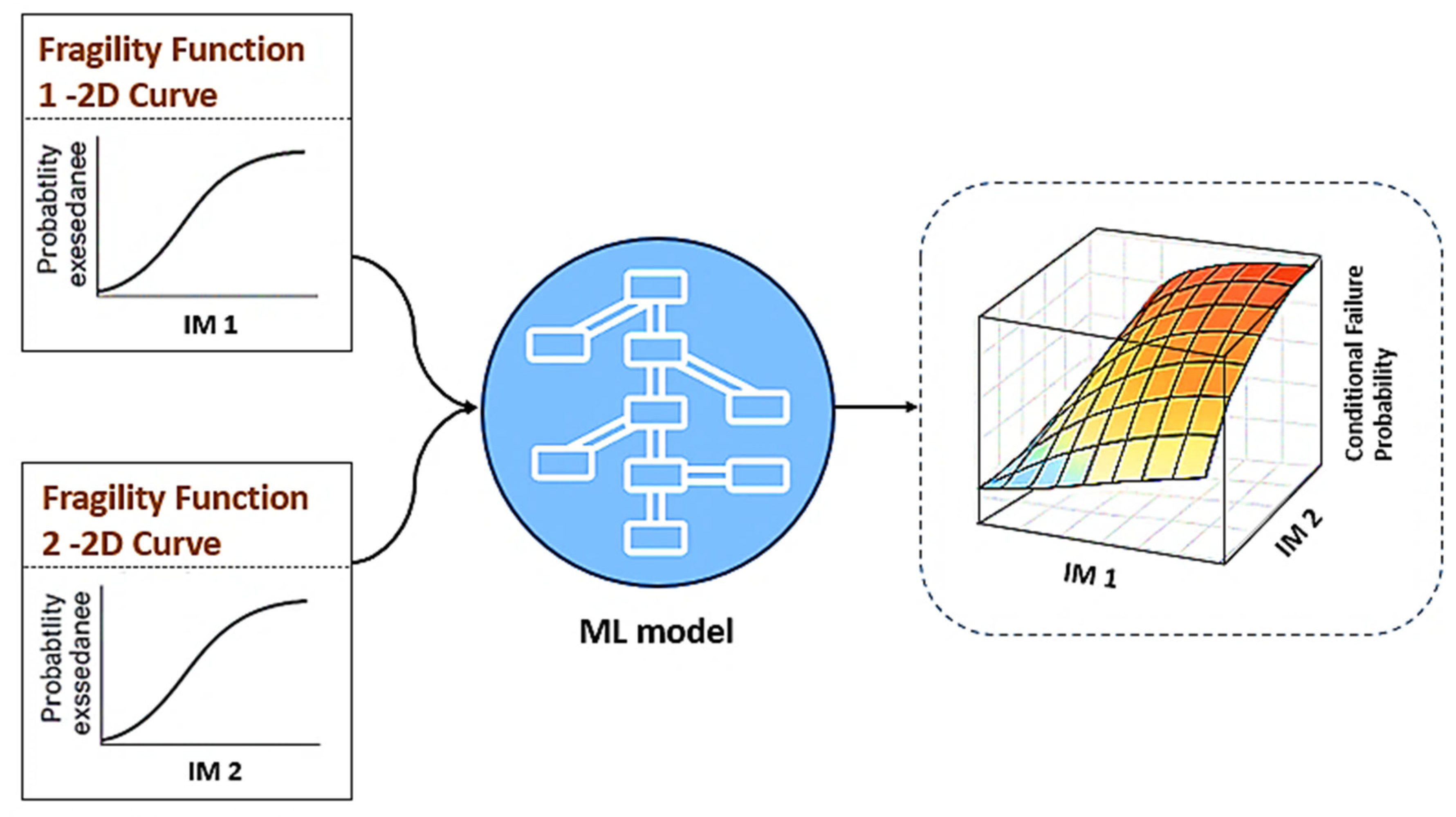
As illustrated schematically in Figure 6, the framework requires two input fragility functions, each expressed as a 2D cumulative probability curve relating a scalar IM to the likelihood of exceeding a specific DS. For the FFE application, the first fragility function represents earthquake-induced collapse probabilities, while the second reflects fire-induced collapse probabilities. These boundary fragility curves are discretized and paired to span the joint hazard space, and their cumulative exceedance probabilities are provided as inputs to the ML model. The output is a synthesized fragility surface P(DS ∣ IM_EQ, IM_Fire), which quantifies the conditional probability of DS exceedance as a function of both hazard intensities.

The central objective of this study is to assess whether fragility surfaces synthesized from the EQ–TS algorithm, when applied to earthquake and fire fragility functions, are consistent with those generated directly from FFE simulation data. Agreement between the synthesized and ML-generated surfaces would validate the EQ–TS methodology as a reliable surrogate for constructing fragility surfaces in new hazard pairings, bypassing the need for extensive sequential analyses. A key advantage of this approach lies in its adaptability: once trained on EQ–TS data, the model can be extended to FFE or other sequential hazards without retraining, provided that the input fragility curves exhibit smooth, monotonic, and bounded cumulative probability behavior [32,78]. This adaptability positions the framework as a scalable tool for resilience assessment, where diverse multi-hazard scenarios can be represented efficiently within a unified fragility modeling architecture.

6. Numerical Illustrations

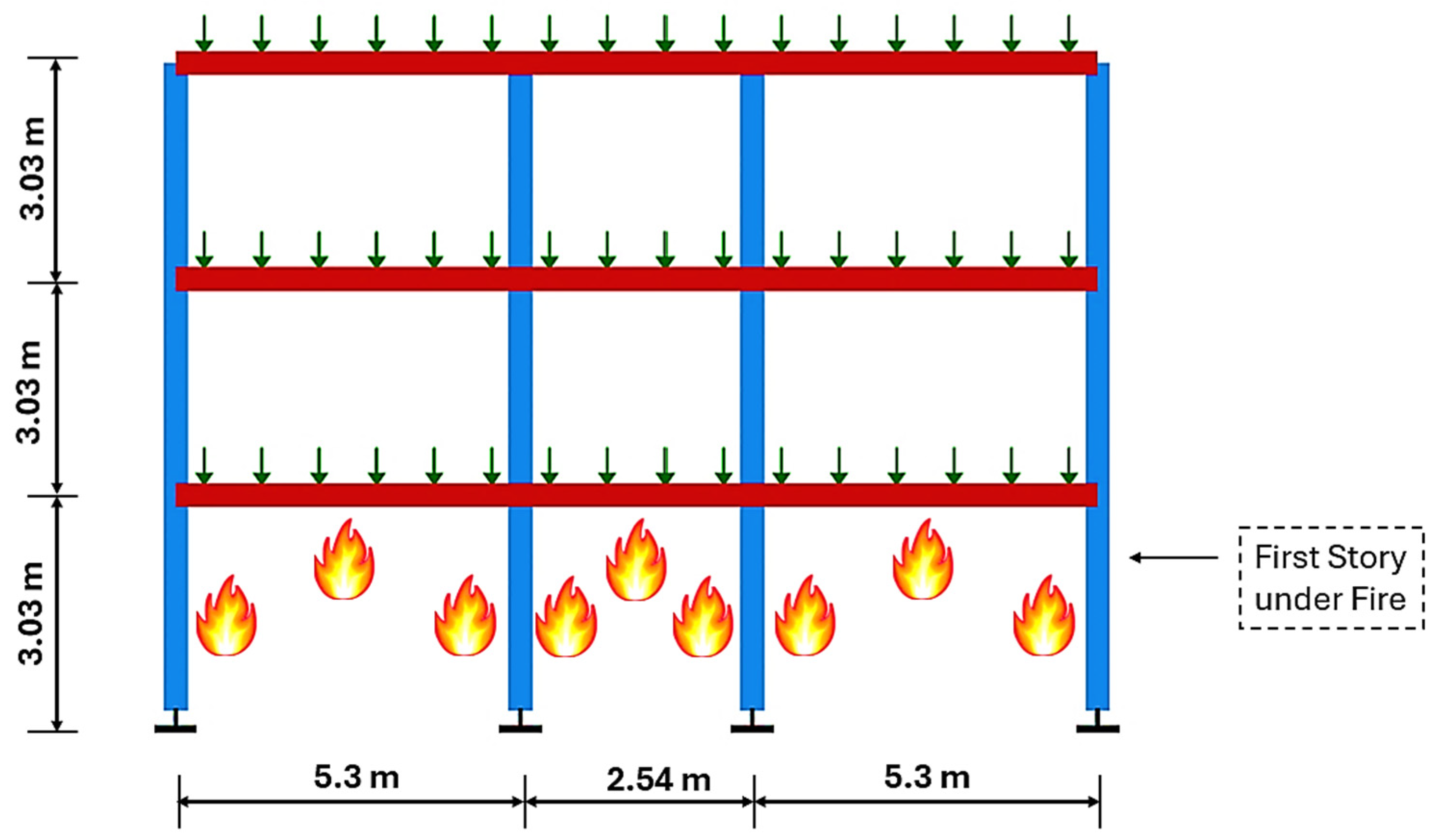
The structure used as an illustrative example is a three-story steel moment-resisting frame representative of a generic office-type building located in a high seismic region of the western United States. The frame is modeled in a two-dimensional (2D) configuration and is adapted from the OpenSeesPy [79] example library. As shown in Figure 7, the frame consists of three bays in the horizontal direction, with each story height set at 3.05 m (10 ft). The bay widths vary along the transverse direction—5.3 m, 2.54 m, and 5.3 m—resulting in an overall building width of approximately 13.2 m (43.3 ft). The span length in the longitudinal direction is 4.9 m (16 ft). For stories not exposed to fire, rigid beam–column end connections are enforced using equal degrees-of-freedom constraints to realistically capture joint behavior. In this case study, only the first story is subjected to fire exposure, while the upper stories remain unheated, consistent with the worst-case fire scenario identified in prior studies [21,23,45,64,65]. However, this uniform heating assumption does not capture localized phenomena such as flame spread or ventilation-controlled burning. In realistic post-earthquake scenarios, partition wall damage can drastically alter ventilation conditions, potentially intensifying fire severity in certain compartments. Therefore, while the adopted modified ISO-834 curve provides computational efficiency and a consistent benchmark, it may underestimate localized thermal effects under realistic ventilation changes, which should be investigated in future studies.

Structural members are modeled using nonlinear displacement-based beam–column elements (described in Section 3) with fiber discretization of W-sections. Columns are modeled with W10 sections, while beams are modeled with W8 sections, with section properties (depth, flange, and web dimensions) corresponding to typical wide-flange members. The fiber-based formulation enables the model to capture both material inelasticity and geometric nonlinearity under combined seismic and fire demands.

This section presents the numerical results obtained by applying the developed framework to the illustrative example building. The simulations capture the interaction between earthquake-induced damage and subsequent fire demands in a probabilistic manner, yielding fire-following-earthquake fragility surfaces. These results provide a basis for evaluating the multi-hazard performance of low-rise MRF systems and serve as the benchmark for assessing the predictive capability of the machine learning framework.

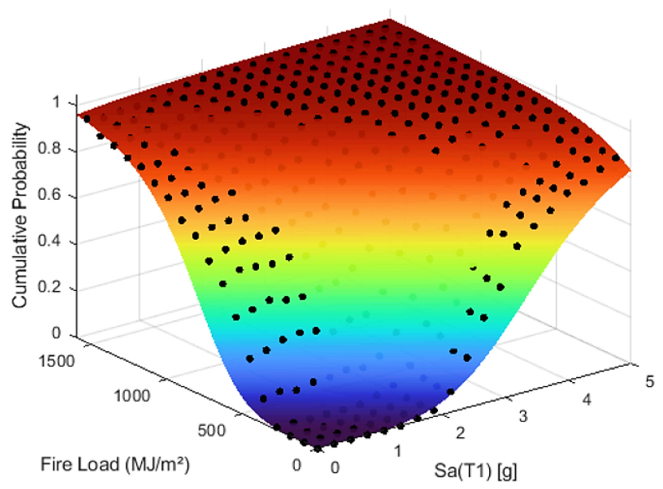
Figure 8 shows the FFE fragility surface developed through the direct simulation methodology for the case study building. The black points represent simulated failure probabilities, while the fitted colored surface illustrates a continuous probabilistic representation of collapse likelihood as a function of earthquake intensity Sa(T₁) and fire load. The agreement between the data points and the fitted surface demonstrates the ability of the successive nonlinear dynamic and thermal analyses to capture joint hazard effects and extend conventional single-hazard fragilities into a unified multi-hazard framework.

The boundaries of the surface yield conventional two-dimensional fragility curves for the earthquake-only and fire-only cases, demonstrating that the proposed sequential simulation framework naturally extends traditional single-hazard fragilities into a unified multi-hazard representation. These findings highlight the capability of the proposed approach to capture both single-hazard performance and the compounding effects of sequential earthquake–fire loading within a unified probabilistic framework. Importantly, the fragility functions and surfaces provide actionable insights for resilience planning and retrofitting strategies, enabling engineers and decision-makers to better evaluate building performance and prioritize mitigation under cascading hazards.

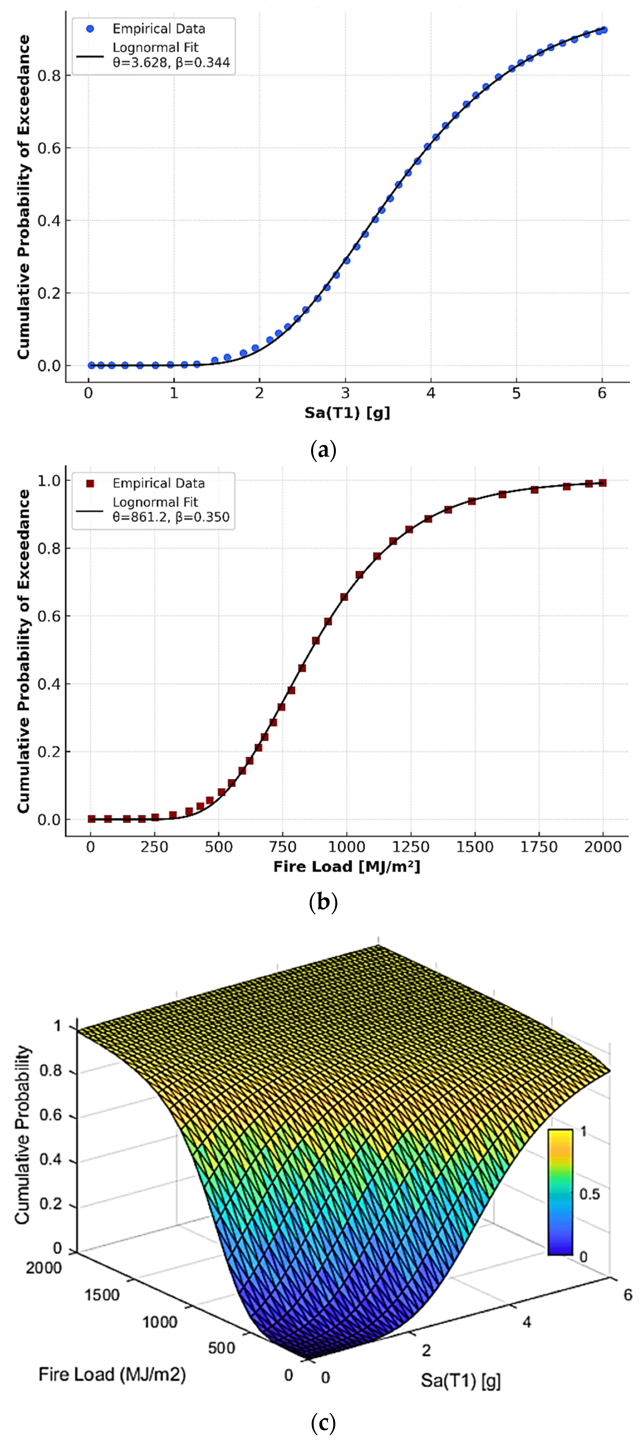
Figure 9 presents the results of the fragility analysis for the case study buildings under single- and multi-hazard conditions. The earthquake-only fragility curve in Figure 9a shows a median capacity of θ = 3.63 g with β = 0.344, while the fire-only curve in Figure 9b yields a median capacity of θ = 861.2 MJ/m² with β = 0.350. Both lognormal fits demonstrate excellent agreement with the simulation data, confirming the robustness of the direct analysis approach. Figure 9c illustrates the ML-generated FFE fragility surface, which transitions smoothly between the earthquake-only and fire-only boundaries and quantifies the probability of exceedance across the full range of joint hazard intensities. The two-dimensional fragility curves and their associated information were extracted from the boundaries of the directly simulated FFE fragility surface shown in Figure 8, and these serve as the input for the ML framework introduced earlier in this paper (Section 5). Using only these boundary fragilities, the ML methodology synthesizes the full FFE fragility surface shown in Figure 9c, which shows excellent consistency with the directly simulated surface.

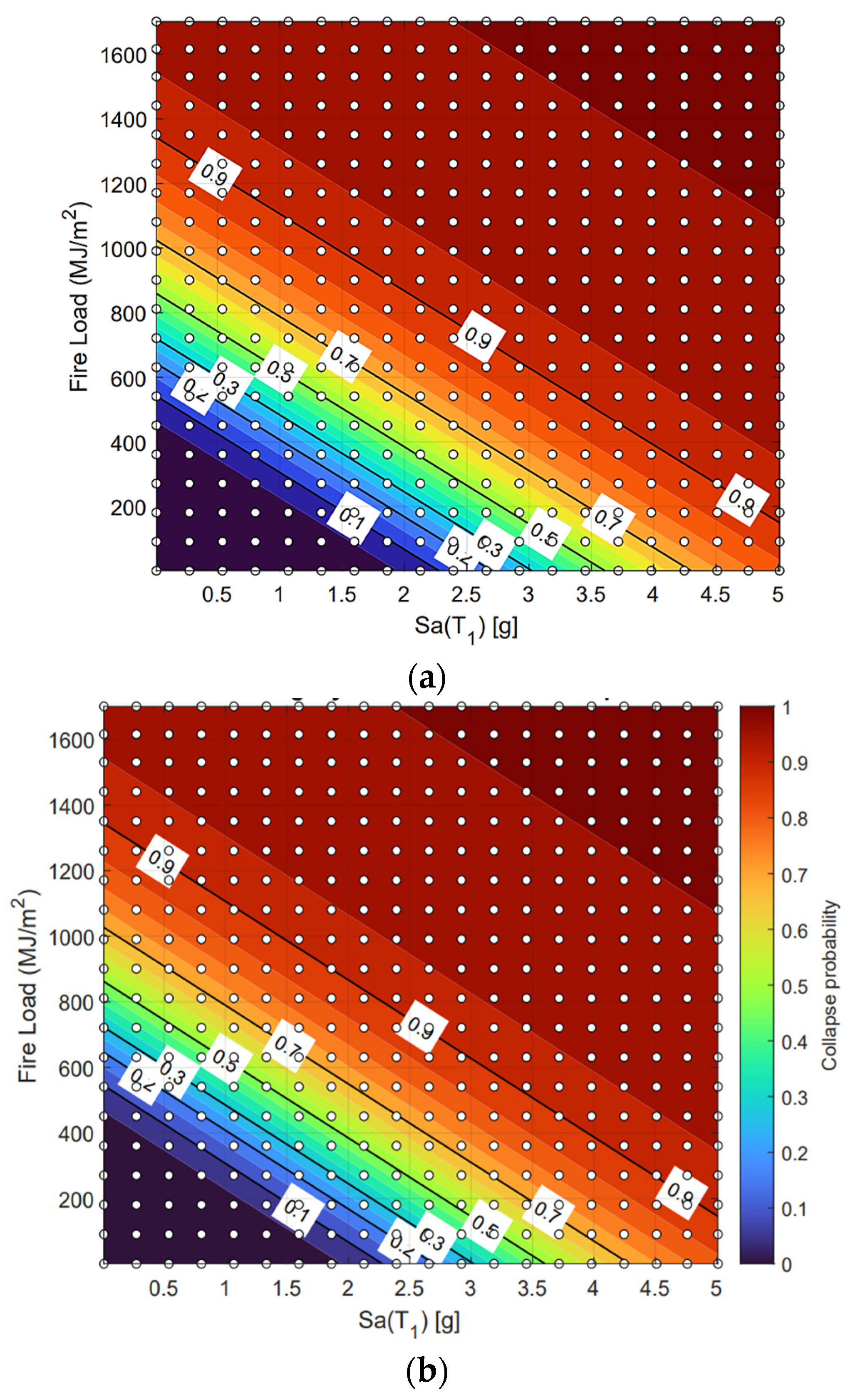
Figure 10 compares the contour representations of the FFE fragility surface, P(DS ∣ IM_EQ, IM_Fire) points, generated from direct successive simulations and the ML-based framework. Figure 10a shows the contour view of the surface obtained through direct analysis, where collapse probability increases smoothly with both earthquake intensity and fire load, and the white contour lines mark probability levels from 0.1 to 0.9. Figure 10b illustrates the contour view of the surface produced by the ML framework using only the boundary fragility curves as input.

As can be seen in Figure 10, the ML-generated surface replicates the key features of the directly simulated surface with high fidelity, including the slope of the probability gradients and the overall shape of the iso-probability contours. This close agreement confirms the capability of the ML approach to synthesize multi-hazard fragility surfaces without requiring extensive successive simulations and even a re-training process, offering substantial computational savings while maintaining accuracy. The ML method provides significant computational savings compared to direct numerical simulation, while maintaining strong agreement with the OpenSees-based reference surfaces. In quantitative terms, the ML-based synthesis required only a few seconds per fragility surface generation on a standard workstation, whereas the full OpenSees-based successive simulation demanded several days of high-performance computing, representing a computational reduction of roughly three orders of magnitude.

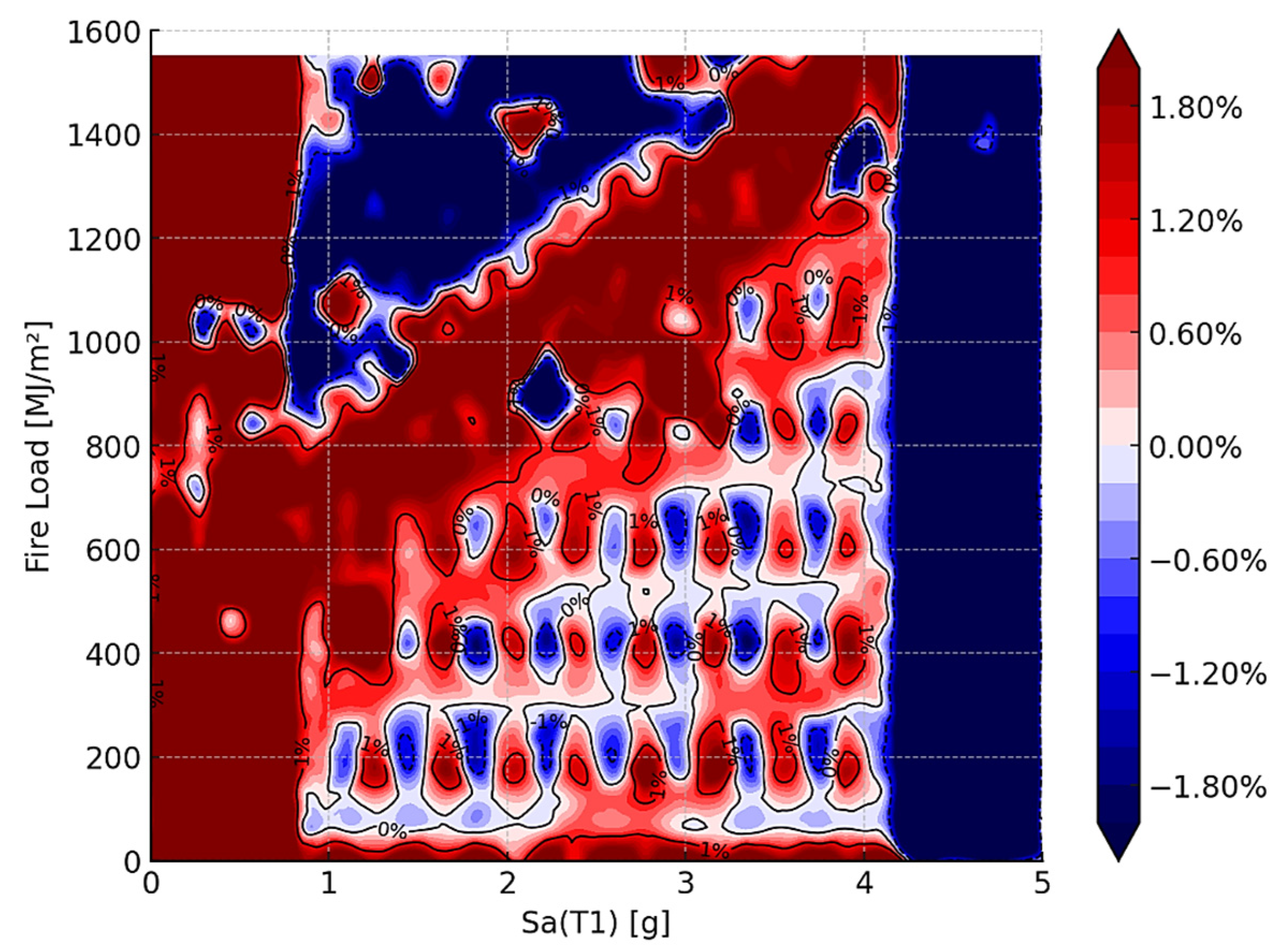
Figure 11 illustrates the difference surface between the ML-based and direct-simulation fragility surfaces, expressed in percentage terms. The contour lines at −1%, 0%, and +1% identify regions of underprediction (blue) and overprediction (red) by the ML framework relative to the benchmark direct-simulation surface. The results indicate that discrepancies remain small across the entire hazard space, generally within ±1%. Localized areas of deviation appear at higher fire load levels combined with moderate seismic intensities, where the ML framework tends to slightly underpredict collapse probabilities. Conversely, minor overprediction is observed at lower fire loads and larger spectral accelerations. Despite these localized differences, the overall agreement is strong, demonstrating that the ML-based framework is able to replicate the direct-simulation surface with high fidelity. Importantly, the ML model achieves this level of accuracy while reducing computational demands significantly, highlighting its suitability for large-scale community-level applications where thousands of hazard scenarios must be evaluated.

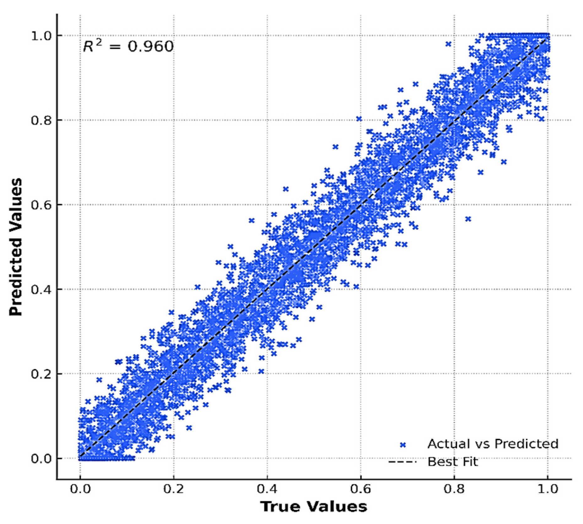
Figure 12 presents a comparison between the ML-predicted fragility values and those obtained from direct simulations (P(DS ∣ IM_EQ, IM_Fire) data points), based on 4000 points sampled from the fitted fragility surface. Each point represents a joint hazard intensity pair of earthquake and fire load, allowing evaluation of model performance across the full multi-hazard domain. The close alignment of the points with the fitted line indicates that the ML framework successfully captures the underlying simulation-based fragility relationships, providing an efficient surrogate for computationally intensive direct analyses. The results demonstrate consistently high predictive accuracy across all cases of joint hazard (IM) values, with R² values exceeding 0.959 and Root Mean Square Error (RMSE) values remaining below 0.018. Mean Absolute Error (MAE) values also remain low, typically within 0.007–0.011, indicating minimal average error across the fragility domain.

Numerical illustrations confirm that the developed framework reliably captures the cascading effects of earthquake and fire in a unified fragility representation for the case study building. The directly simulated FFE surfaces provide a robust benchmark for evaluating hazard interaction, while the machine learning framework demonstrates its ability to reproduce these results with high fidelity and significantly reduced computational demand. In this way, an FFE fragility surface can be constructed using available two-dimensional fragility curves for earthquake-only and fire-only hazards, enabling the use of the rich and well-established fragility or vulnerability functions already available for individual hazards in the literature. Together, the two approaches highlight a practical pathway for integrating simulation-based rigor with ML-driven efficiency, offering scalable, probabilistically consistent tools for structural performance assessment and resilience-oriented decision making under multi-hazard scenarios.

7. Summary and Conclusions

This study presented an integrated framework combining high-fidelity simulation and machine learning to generate fire-following-earthquake fragility surfaces for a steel moment-resisting frame. The proposed ML approach accurately reproduced the coupled hazard response predicted by nonlinear OpenSees analyses while reducing computational demand by several orders of magnitude. The framework demonstrates strong adaptability across multi-hazard sequences and provides a foundation for future extensions to other hazard pairings and structural systems.

The methodology was benchmarked against a machine learning synthesis framework originally developed for earthquake–tsunami sequences and extended here to earthquake–fire hazards. This framework, previously validated for mainshock–aftershock sequences, demonstrates robustness across different types of sequential hazards. Numerical results for a three-story steel MRF showed excellent agreement between simulated and ML-synthesized fragility surfaces, with a coefficient of determination (R²) exceeding 0.95 and a root mean square error (RMSE) below 0.02 across all damage states. These results confirm not only the computational efficiency and predictive accuracy of the ML framework but also its apparent hazard-neutrality, as the same architecture can be effectively applied across diverse hazard pairings—earthquake–tsunami, mainshock–aftershock, and fire-following-earthquake—without retraining.

Beyond methodological development, the results of this study have direct implications for industry, federal agencies and research. For practicing engineers and consultants, the fragility surfaces generated through this framework can provide insights for performance-based design and retrofit decisions, especially for structures exposed to compound hazards. For policymakers and decision-makers, the ability to capture uncertainty and cascading effects within a unified fragility representation provides a powerful tool for risk assessment, emergency planning, and resilience-based policy development. In the research domain, the framework offers a benchmark for validating new modeling approaches and serves as a foundation for expanding fragility methodologies to community-scale resilience studies. The integration with ML further opens opportunities for rapid hazard assessment tools that can be embedded in next-generation catastrophe risk models and infrastructure digital twins like IN-CORE platform.

Despite its contributions, the methodology presented in this study is subject to several limitations that should be acknowledged and addressed in future work. First, the fire hazard was represented using the ISO-834 standard curve with stochastic modifications, which, while computationally efficient, may not capture localized or ventilation-controlled fire dynamics; future studies could incorporate more physically based fire models. Second, the case study was limited to a three-story steel MRF, and extension to taller buildings, different structural typologies, and irregular geometries is needed to evaluate broader applicability. Although the present investigation focused on a single structural configuration and a representative fire scenario, the findings consistently support the proposed methodology, and broader validation across diverse building types and fire conditions will strengthen its generality. Third, uncertainties in thermal–mechanical material properties were treated in a simplified manner, and temperature-dependent degradation models could be expanded using experimental calibration. Finally, while the ML framework demonstrated strong hazard-neutral adaptability, its extrapolation to hazard pairings with fundamentally different fragility curve characteristics (e.g., abrupt slope changes or discontinuities) remains untested, referring to both hazard pairings and structural behaviors that yield fragility curves with abrupt slope changes or discontinuities due to highly nonlinear or threshold-type responses. Additionally, the ML framework’s performance has not yet been validated for other sequential hazard pairings (e.g., wind–surge and flood–earthquake) or for irregular and high-rise structural configurations, which may exhibit distinct interaction mechanisms. Future work should explore these extensions to assess the model’s generalizability across a broader range of structural and hazard conditions. Future research should explore these extensions to enhance the robustness, generality, and practical deployment of the methodology.