Comparison of Methods for Reconstructing Irregular Surfaces from Point Clouds of Digital Terrain Models in Developing a Computer-Aided Design Model for Rapid Prototyping Technology

Abstract

This article presents a methodology for developing a three-dimensional terrain model based on numerical data in the form of a point cloud, with an emphasis on reducing mesh surface errors and using a surface smoothing factor. Initial surface generation was based on a point cloud with a square mesh, and an adopted algorithm for mesh conversion to the input form for the computer aided design (CAD) environment was presented. The use of a bilinear interpolation algorithm was proposed to reduce defects in the three-dimensional surface created in the reverse engineering process. The terrain mapping accuracy analyses were performed for three samples of different geometry using two available options in the Siemens NX program. All obtained surfaces were subjected to shape deviation analysis. For each of the analyzed surfaces, changing the smoothing factor from 0% to 15% did not cause significant changes in accuracy depending on the method adopted. For flat regions, in the Uniform Density (UD) method, the size of the area outside the tolerance was 6.16%, and in the Variable Density (VD) method, it was within the range of 5.01–6%. For steep regions, in the UD method, it was 6.25%, and in the VD method, it was within the range of 5.39–6.47%, while for concave–convex regions, in the UD method, it was 6.5% and in the VD method, it was within the range of 4.96–6.36%. For a smoothing factor value of 20%, a sudden increase in the inaccuracy of the shape of the obtained surface was observed. For flat regions, in the Uniform Density (UD) method, the size of the area outside the tolerance was 69.84%, and in the Variable Density (VD) method, it was 71.62%. For steep regions, in the UD method, it was 76.07%, and in the VD method, it was 80.94%, while for concave–convex regions, in the UD method, it was 56.08%, and in the VD method, it was 62.38%. The developed methodology provided high accuracy in the reproduction of numerical data that can be used for further analyses and manufacturing processes, such as 3D printing. Based on the obtained data, three fused deposition model (FDM) prints were made, presenting each of the analyzed types of terrain geometry. Only FDM printing was used, and other technologies were not verified.

1. Introduction

For many years, reverse engineering has been playing a key role as an irreplaceable tool in the processes of obtaining data on existing objects and their digital processing, as well as producing physical copies of these elements. It is used in numerous fields, from the automotive and aerospace industries to biomedical engineering. Especially in combination with additive technologies, such as 3D printing, reconstructive engineering is becoming a basic tool used in the reproduction and production of mechanical parts that may be difficult or impossible to obtain using traditional production methods [1].

The basic method of reconstructing simple elements, such as those presented by Budzik et al. [1], is to map a point cloud by using an approximation through simple solids (cylinder, cone, sphere). In the case of more complex but still regular surfaces, a mapping using free surfaces described by polynomials for both the U and V directions of the surface or a B-spline surface is used [2].

Progress in the field of precise measurement methods, as well as the development of new measurement technologies and data acquisition systems, such as computed tomography, 3D laser scanning, and digital photogrammetry, has allowed for a significant expansion of the possibilities of reconstructive engineering. Thanks to these technologies, it has become possible to accurately reproduce not only simple mechanical elements with regular geometry but also complex biological structures characterized by a high degree of irregularity and complexity of shapes [3,4,5]. This has opened up new perspectives in fields such as medicine, archaeology, or the protection of cultural heritage, in which the faithful reconstruction of biological or historical structures is of key importance.

A special case of a reverse engineering application is the reconstruction of large-scale objects, which include, among others, topography, extensive geological formations, and large engineering structures [6,7]. The process of digitizing such objects brings with it additional challenges related to their size and the variety of surfaces. For this reason, not all available imaging and measurement technologies are able to meet the requirements for the accuracy and efficiency of data acquisition.

The basic measurement methods currently used in obtaining topographic data include light detection and ranging (LiDAR) technology, photogrammetry, satellite measurements, and ground measurements via the global positioning system (GPS). Each of these methods is characterized by different principles of operation, ranges of applications, and accuracies, which allows for their appropriate selection depending on the specifics of the project and terrain conditions [8].

The LiDAR measurement method is used with great success to generate precise three-dimensional point clouds that represent existing objects and terrain surfaces. Thanks to the use of laser pulses and the precise measurement of their return time, it is possible to obtain very detailed representations, even in difficult environmental conditions, for example, in densely forested areas. Depending on the measurement purpose, the size of the digitized objects, and the possibility of physical access to them by operators, different variants of this technology are used. For data acquisition on a smaller scale, in hard-to-reach places, terrestrial LiDAR systems are used, as described in the literature [7,8,9]. On the other hand, if it is necessary to cover large areas, systems mounted onboard flying vehicles, such as airplanes or unmanned aerial vehicles [10], are used.

Data from LiDAR are supplemented by elevation measurements performed using GPS receivers, which enable the direct verification and calibration of field measurement results [11]. In particular, high-accuracy geodetic techniques are used, such as the global navigation satellite system (GNSS) or static measurements, which increase the precision of localization of the acquired spatial data.

In parallel to LiDAR technology, photogrammetry is also often used, i.e., a technique for obtaining information about objects and their spatial arrangement based on photo analysis. Photogrammetry, using photos taken from different perspectives, allows for the reconstruction of three-dimensional surface geometry. Due to significantly lower implementation costs compared to LiDAR systems, photogrammetry is widely used in projects in which maintaining the cost-effectiveness ratio is important. Currently, the main carriers of imaging sensors are drones, which, thanks to their mobility and operational flexibility, allow for the capture of high-resolution photos in various terrain conditions [12,13].

In addition, measurement techniques based on satellite observations are used to obtain data on the terrain. Satellite measurement allows for the quick collection of information on very large areas, which is particularly useful in regional and global studies. One of the most popular methods is the use of data from the Advanced Spaceborne Thermal Emission and Reflection Radiometer (ASTER) system, as presented in [14,15]. Alganci et al. [16] present a detailed comparison of various satellite measurement methods, analyzing their accuracy, scope of application, and limitations.

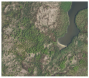
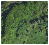
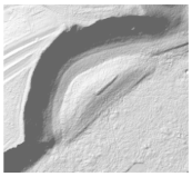
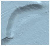
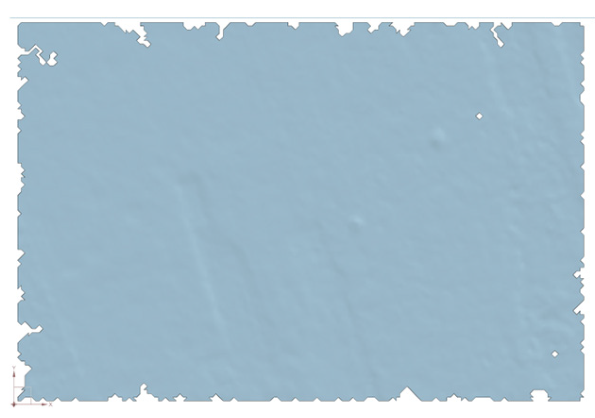
The final effect of using the described measurement methods is the creation of a digital surface model (DSM). This model represents a point cloud that contains information on both the terrain proper and the elements located above the ground surface, such as vegetation, buildings, and other anthropogenic structures, as shown in Figure 1. DSM is the basis for further spatial analyses, the modeling of the natural environment, urban planning, and the monitoring of changes in the landscape.

A separate challenge is how to filter out objects located above the terrain geometry, i.e., vegetation and buildings, which are an integral part of DSM data. In the process of creating a digital terrain model (DTM), advanced real-time data reduction techniques are increasingly used. One example is the optimum dataset method (OptD) [17], which allows for the generation of DTMs in parallel with data acquisition. Thanks to sequential estimation and dynamic data reduction, this method preserves the most important terrain features while significantly reducing the volume of data by up to 98%, without any significant loss of accuracy. This approach significantly increases computational efficiency and allows for the ongoing creation of 3D models with high precision, which is of great importance in applications that require fast data processing.

In parallel, classical LiDAR point cloud filtering algorithms are being developed. Six popular methods, including the adaptive triangulated irregular network (ATIN), elevation threshold with an expanded window (ETEW), maximum local slope (MLS), progressive morphology (PM), iterative polynomial fitting (IPF), and multiscale curvature classification (MCC), were tested, each showing different levels of effectiveness depending on the terrain characteristics [18,19]. IPF achieved the best results for flat and urban areas, while ETEW was the most effective in difficult, mountainous areas with dense vegetation. Zhang et al. [20] and Lee et al. [21] focused on the challenges associated with filtering photogrammetry data using the digital surface model (DIM) and structure from motion (SfM) methods. Classic LiDAR filters can be partially effective for DIM data but require additional procedures, such as a ranking filter, to minimize systematic errors. In SfM applications, especially for riverine areas, combining vegetation filters, such as normalized difference vegetation index (NDVI) and excess green (ExG), with morphological filters, such as cloth simulation filtering (CSF) and ATIN, has proven effective, thereby improving model quality while maintaining low operating costs.

A separate category of methods is techniques based on object segmentation, as described by Song et al. [22]. The novel approach assumes defining objects as areas enclosed by steep slopes and the ground as smoothly connected spaces, which allows for more consistent filtering over large areas, especially in the urban environment. Additionally, including water bodies and artificial structures, such as bridges, increases the realism of the obtained models. Traditional procedures [23], which are used within the GRASS Geographic Information System (GIS), remain effective in the basic classification of LiDAR data, rejecting buildings and vegetation in order to obtain a precise DTM. Modern filtering approaches increasingly combine several methods to achieve the highest possible model accuracy in diverse terrain conditions.

A separate problem is the noise and irregularity of measurement data, which cause errors in the correct reconstruction of the complex surface. Marton et al., in their article [24], presented a method for filling in missing measurement points using the resampling method. Here, the method of weighted least squares was used to fill in missing data in real time.

The current article presents research indicating the possibility of effective processing of geodetic data and the use of mesh surface creation techniques in the CAD and computer-aided engineering (CAE) environment to prepare models made using 3D printing. The key aim of the publication was to show the entire process of creating a model, from the analysis of input data through the densification of the point grid, which allowed us to reduce errors in creating surfaces, to the use of CAD tools to obtain a digital representation of the surface, ending with obtaining a physical model made via 3D printing. Unlike the method presented by Marton et al. [24], the densification of the point cloud did not consist of filling in the missing areas of the mesh but of creating nodes that facilitate the reconstruction of the surface based on measurement data.

Such models have practical applications, among others, in special education or geoengineering. The research was carried out on three types of surfaces that represented relatively flat surfaces, which had steep slopes and contained concave–convex forms. An algorithm was developed to increase the quality of the conversion of geodetic data to the mesh surface. The numerical analyses performed allowed for the assessment of the impact of different mesh generation methods and smoothing functions on the accuracy of mapping the terrain topography.

2. Materials and Methods

2.1. Input Data and Their Characteristics

The point cloud, which is the basis of the digital terrain model (DTM), was developed in the form of an ordered grid of regular rectangles with a constant cell size of 1 × 1 m. This type of spatial data structure allows for the precise analysis of the terrain morphology and further numerical processing, such as surface runoff modeling, slope inclination analysis, or the generation of terrain profiles. The numerical data used to build the model were obtained from a publicly available source: the Geoportal application [25], which is managed by the Head Office of Geodesy and Cartography in Poland.

The applied elevation data refer to the currently applicable national elevation reference system PL-EVRF2007-NH, which is the Polish implementation of the European Height Reference System. This system was officially introduced in Poland by the Regulation of the Council of Ministers Dz.U.2024.0.342 §24 [26] on 1 January 2024, replacing the previous PL-KRON86-NH system. This change aims to unify elevation references on an international scale and ensure compliance with European geodetic and hydrographic standards. Thanks to this change, the elevation data used in spatial analyses are characterized by greater consistency and precision, which is particularly important in the context of data integration at the international level.

The point cloud representing the topography of the analyzed terrain area was obtained in American Standard Code for Information Interchange (ASCII) text file format. This file contains data in the form of a two-dimensional matrix with dimensions of y × x, in which each cell corresponds to the height value of the measured terrain point relative to the adopted reference system. Such an organized data structure allows for the basic visualization of the surface shape but encounters significant limitations in the context of reconstructive engineering applications.

2.2. Transforming Input Data

When using professional reconstructive engineering tools such as Siemens NX in version 23.06.3001 or other CAD/CAE software, the matrix format is not optimal or natively supported as an input database. The main problems resulting from this data structure are as follows:

• The first is the reversal of the orientation of the y-axis corresponding to the north (N) geographic direction. In an ASCII file, data are most often ordered in a way that maps the direction from north to south, which means that the increasing values in the matrix rows correspond to the south (S) direction, not N. This leads to a discrepancy with the spatial orientation expected by engineering software, which interprets the axes in accordance with Cartesian systems (x-width, y-length, and z-height).
• The second is the inappropriate data storage format. Most engineering applications, including NX, expect data in the form of a set of three-dimensional coordinates of points in the format of x; y; z, where each line contains three values: coordinates x and y and the corresponding height, z. A specific storage convention is also required, most often using a field separator in the form of a semicolon (;) or a comma, depending on the regional settings and program requirements.

For this reason, it is necessary to first convert the data from the matrix format to a list of points in the x; y; z format. This process requires taking into account the grid size (e.g., 1 × 1 m) and the order of rows and columns, as well as shifting or correcting the y-axis orientation in order to adapt the system to the CAD system requirements. Only after such a conversion can the data be effectively imported and used in the process of creating surface or solid models in engineering environments.

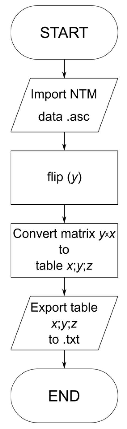
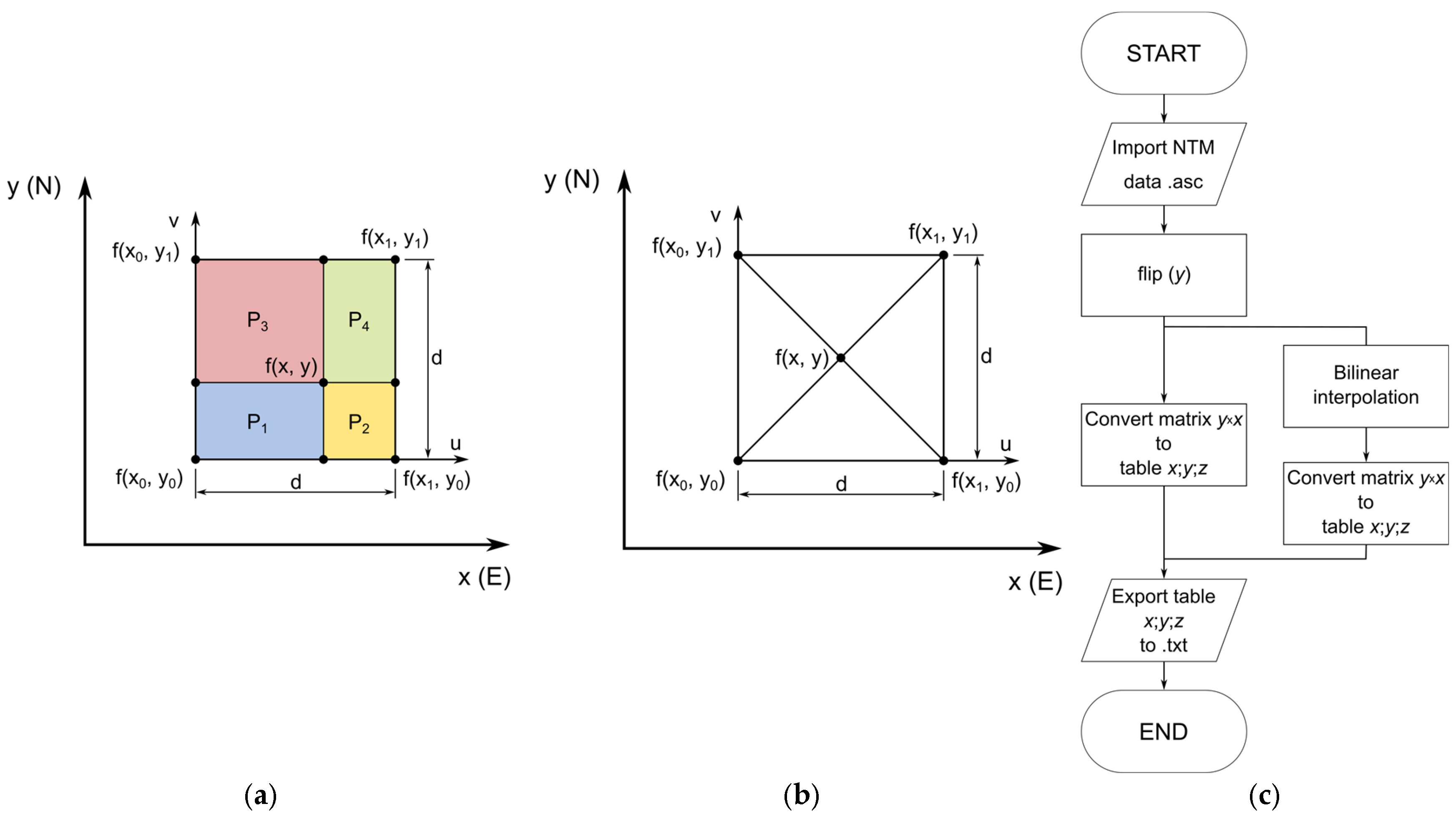
In order to adapt the numerical data to CAD software standards, a program was created to convert the y × x matrix into the x; y; z data format and to reverse the y-axis direction. The schematic diagram of the algorithm is shown in Figure 2.

After the necessary data conversion from the matrix format to the point coordinate format, x; y; z, the point cloud was imported into the design environment of Siemens NX software, which is an advanced CAD tool that is used, among others, in reverse engineering and surface modeling. The aim of the operation was to reconstruct the terrain topography based on the acquired measurement data.

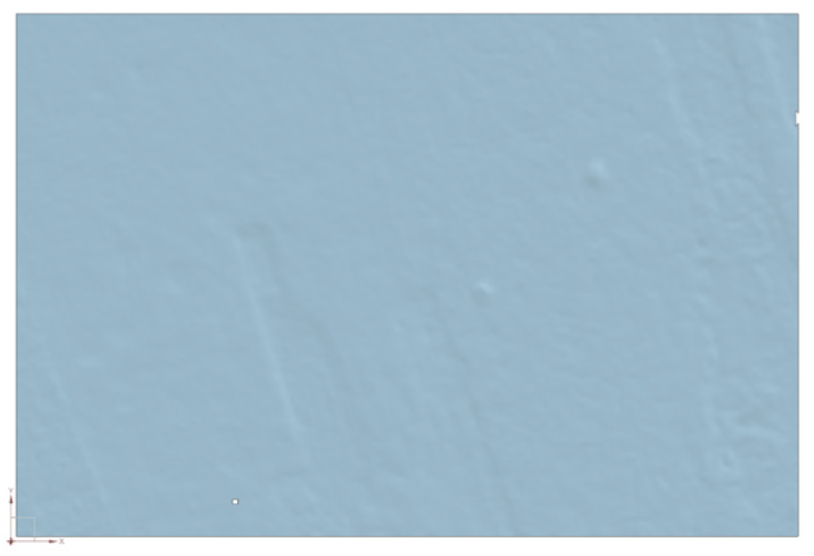
The surface reconstruction process began with the use of tools for creating a surface composed of a triangle mesh based on imported points. Although the base mesh had a regular square layout of 1 × 1 m, which should theoretically help to obtain a uniform surface, a number of undesirable effects were encountered due to the limitations of the meshing algorithms and the nature of the input data.

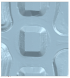
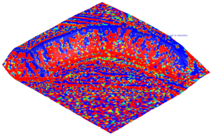
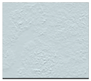
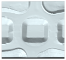
During surface reconstruction, numerous geometric artifacts appeared in Figure 3, including:

• gaps and discontinuities in the mesh, leading to the creation of empty areas (holes) in the model;
• holes and gaps at the edges, resulting from the lack of clear neighbors for boundary points;
• notches and surface breaks appearing in places where the point data were irregular or insufficiently dense;
• overlapping mesh triangles, i.e., topological errors resulting in surface intersection and generating geometry that is mathematically incorrect and difficult to further process.

Figure 3. Defects created on a surface generated from a square grid of points.

Figure 3. Defects created on a surface generated from a square grid of points.

All of the errors listed significantly affect the quality and usability of the obtained terrain reconstruction, thereby limiting the possibilities of using the model in further design stages. The identified problems indicate the need for the prior cleaning and preparation of the point cloud, including smoothing the surface, interpolating missing data, and using dedicated reconstruction algorithms, which are better adapted to work with regular grids with a large number of points.

2.3. Application of the Bilinear Interpolation Algorithm

In order to improve the quality of the generated surface and reduce the number of topological errors that occur during the surfacing process, it was decided to use the bilinear interpolation technique at the central points of each cell of the base grid, as shown in Figure 4a.

The bilinear interpolation algorithm was based on the input points in ASCII format for a d × d grid resolution. Therefore, an element performing bilinear interpolation was added to the basic algorithm (Figure 4c). The bilinear interpolation equation is presented in Formula (1) [27,28], where the coefficients, f(x_i, y_i), correspond to the height value, z, at a given grid point (Figure 4a,b).

$$f\left(x,y\right)={\displaystyle \frac{f\left(x_0{,y}_0\right)·\left(d-x\right)·\left(d-y\right)+f\left(x_1{,y}_0\right)·x·\left(d-y\right)}{d^2}}+{\displaystyle \frac{f\left(x_0{,y}_1\right)·\left(d-x\right)·y+f\left(x_1{,y}_1\right)·x·y}{d^2}}$$

(1)

In order to simplify the algorithm, the formula was transformed by replacing the factors, f(x_i, y_i), with the parameter, zi, and the remaining factors with the parameters, Pi (2, 3).

$$\begin{gathered} P_1=x·y{, P}_2=\left(d-x\right)·y, P_3=x·\left(d-y\right),P_4=\left(d-x\right)·\left(d-y\right) \\ {z}_1=f\left(x_0{,y}_0\right),z_2=f\left(x_1{,y}_0\right),z_3=f\left(x_0{,y}_1\right),z_4=f\left(x_1{,y}_1\right) \end{gathered}$$

(2)

$$f\left(x,y\right)={\displaystyle \frac{z_1·P_4+z_2·P_3+z_3·P_2·y+z_4·P_1}{d^2}}$$

(3)

The parameter d² was replaced by the sum of the surface areas of the individual segments, P_i (4), thereby obtaining Equation (5).

$$d^2=P_1+P_2+P_3+P_4$$

(4)

$$f\left(x,y\right)={\displaystyle \frac{\sum _{i=1}^4{z}_i·P_i}{\sum _{i=1}^4{P}_i}}$$

(5)

The original grid, which was made of regular 1 × 1 m squares, was thus transformed into a system containing additional nodes located exactly at the geometric centers of each square cell.

Bilinear interpolation involves determining the height value, z, at the central point of the grid cell based on the values measured at the four corner nodes of the given mesh. This is an estimation method that assumes a linear change in the values along the x and y axes, which allows for smoother transitions between points and reduces local height jumps. This made it possible to generate a more continuous and coherent terrain surface.

After determining the center points, each square grid cell was divided into four triangles, connecting the corner nodes with the newly determined center point Figure 4b. This approach allowed for the replacement of the square grid with a mesh with an exclusive triangular division, which significantly increased the stability and accuracy of the CAD surface creation algorithms. Triangular elements are more resistant to errors related to the nonplanarity of a surface and better represent terrain irregularities.

It should be noted that bilinear interpolation is only a basic resampling tool. It does not increase the resolution of the mesh itself, and the coordinates of points created during its implementation are burdened with errors, as described by Hu et al. in [26]. However, in the conducted research, bilinear interpolation was used to increase the efficiency of the tool that created surfaces in the CAD environment, which is ultimately based on a triangular grid. The only solution that would exclude the use of bilinear interpolation in the studied case would be to perform an additional measurement of the real terrain, which would fill in the missing grid points.

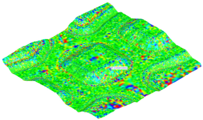
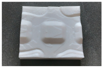
The use of this method contributed to a significant reduction in the number of reconstruction errors, including a reduction in the number of holes and overlapping surfaces (Figure 5).

2.4. Generating Surfaces for Comparison

As part of the experiment, to check the correct operation of the above-described method and to compare the accuracy of surfaces generated with different settings of the Mesh Point Cloud tool, three areas are presented in

Table 1. Comparison of visualization methods for three selected research areas.

Type of Surface Area Size x;y	Orthophotomap	Shading	3D Surface
flat region 180; 158 m
steep region 170; 156 m
concave-convex region 121; 133 m

.

The surface for each area was generated using the following three methods, which are available in NX software [29]:

• Keep All Points;
• Variable Density (VD);
• Uniform Density (UD).

The Keep All Points method is the simplest to operate and involves creating a surface from a triangle mesh between all the points in the cloud. The Variable Density method creates larger segments from the point cloud in regions of low curvature and smaller segments in regions of high curvature. The Uniform Density method creates a surface from the point cloud with a grid of equal-area triangles.

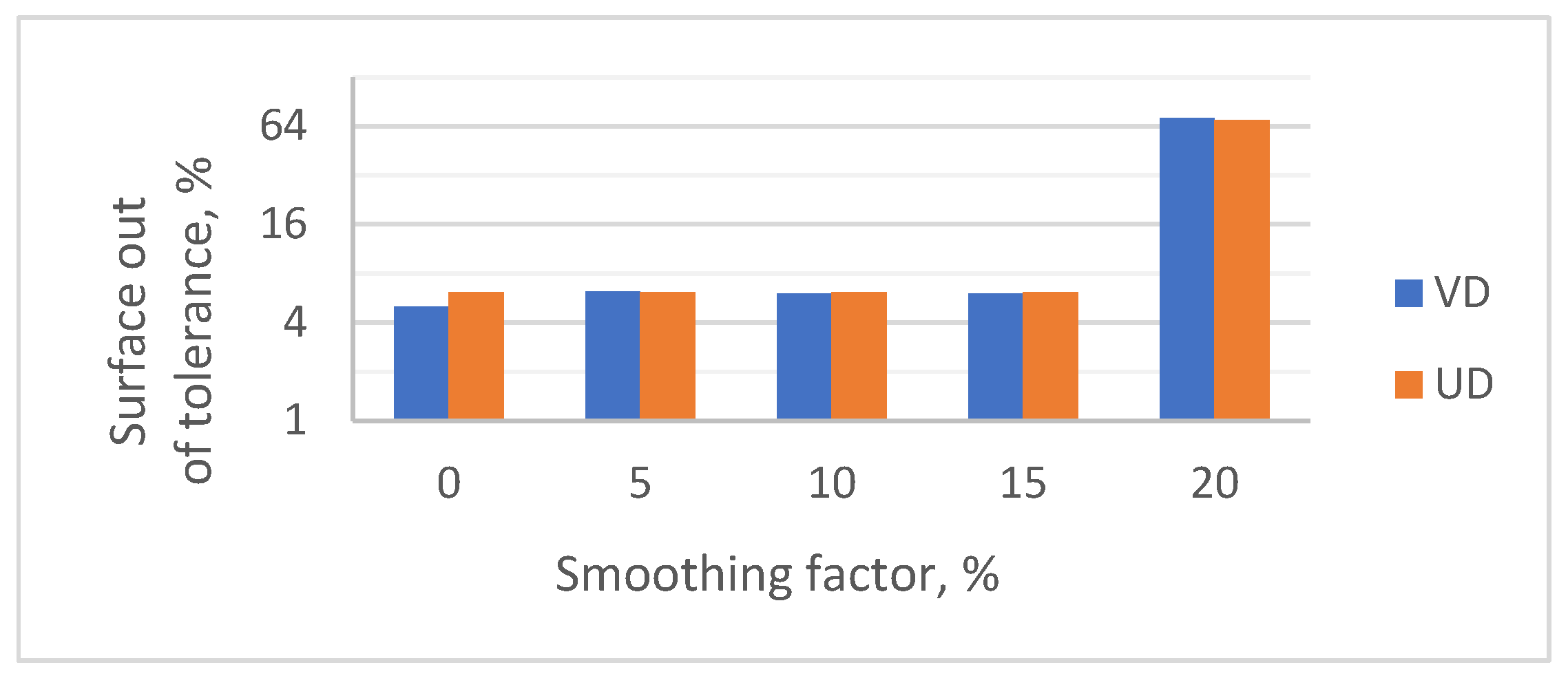
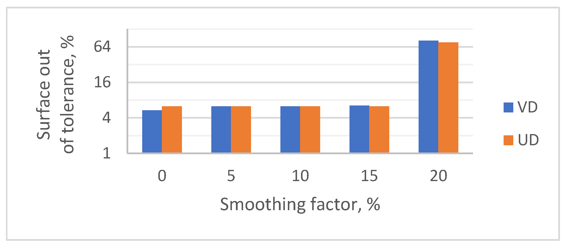
The Keep All Points method was chosen to create a reference surface due to the most accurate rendering of the imported point cloud; however, it does not have a surface smoothing tool. In the other methods, the surface smoothing factor is present, and during the comparative tests, five values were adopted for it: 0, 5, 10, 15, 20%.

3. Results

3.1. Comparative Analysis of Surface Creation Tools

In order to reduce the data size, a 1 × 1 m resolution real grid was imported into the CAD software at a resolution of 1 × 1 mm. The surface shape tolerance was set at ±0.01 mm.

The simulations performed showed slight differences in the accuracy of surface reconstruction depending on the degree of smoothing, ranging from 0% to 15%.

For flat areas, the percentage of areas outside the tolerance range for Variable Density surfaces ranged from 5.01% to 6.17%. For Uniform Density surfaces, the value was 6.16%, as shown in Figure 6.

In the steep regions, the Variable Density surface showed deviations in the range of 5.39–6.47%. In the Uniform Density surface, 6.25% of the surface was out of tolerance, as shown in Figure 7.

For the concave–convex regions, the Variable Density surface deviation ranged from 4.96 to 6.44%, while the Uniform Density surface reached 6.5% of the surface out of tolerance (also shown in Figure 8).

For all analyzed cases and surface types, the application of 20% smoothing resulted in a significant deterioration in the accuracy of the geometry representation. The highest percentage deviation was recorded for the steep region for the Variable Density surface, while the lowest was recorded for the Uniform Density surface in the concave–convex region (Figure 8).

In general, it has been found that at 20% smoothing, Uniform Density surfaces provide a greater proportion of surface area within tolerance than Variable Density surfaces.

Additionally, surface deviation maps that graphically present areas that exceed the permissible tolerance range were developed (

Table 2. Surface deviation map for the flat region.

Smoothing, %	Variable Density	Uniform Density	Scale
0			mm
5
10
15
20

,

Table 3. Surface deviation map for the steep region.

Smoothing, %	Variable Density	Uniform Density	Scale
0			mm
5
10
15
20

and

Table 4. Surface deviation map for the concave–convex region.

Smoothing, %	Variable Density	Uniform Density	Scale
0			mm
5
10
15
20

).

For flat surfaces in both cases—Uniform and Variable—the distribution of out-of-tolerance areas was scattered and random (Table 2).

In the case of steep and concave–convex regions in the Variable Density method, most of the deviations were located in places with a relatively constant curvature (Table 3 and Table 4). In the case of the Uniform Density method, the largest clusters of areas outside the tolerance occurred in transitional regions on the boundaries of surfaces with different inclinations.

3.2. Three-Dimensional Printing Based on the Proposed Methodology

The next stage of the research focused on transforming the previously generated surface into a stereolithography (STL) model, which was then used to produce physical models using the additive method, also known as 3D printing. The STL file was exported from NX as a binary file with parameters ensuring the highest accuracy. The Chordal Tolerance parameter was set at 0.0025 mm, and the Angular Tolerance parameter was set at 1.000 deg. The aim of this stage was to verify the possibility of mapping selected terrain structures in the form of real models using additive technology.

The surfaces that showed the highest percentage of the area within the tolerance range were selected for further analysis and testing, meaning that they were most consistent with the expected topographic profile. In each case, this was a sample created using the Variable Density tool with a smoothing factor of 0% applied, thereby preserving the original detail of the input data.

The models were printed using FDM technology using the Fortus 360mc (Stratasys, Eden Prairie, MN, USA) printer, which has a workspace of 406 × 355 × 406 mm (Figure 9). The model material was PC-10 polycarbonate, which is characterized by good mechanical strength and thermal resistance, making it suitable for mapping complex terrain forms. The support material was PC-S, which allows for the precise printing of even complex geometries, thanks to its easy removal after the process is completed.

In order to obtain the appropriate print quality, a nozzle marked with the symbol T12 was used, which allowed us to achieve a single layer of filament thickness of 0.178 mm. As a result of the work carried out, three physical models were obtained, each of which corresponded to one of the distinguished types of terrain morphology (

Table 5. Presentation of the STL virtual model and the real body.

Types of Terrain	STL Body	Printed Body
flat region
steep region
concave-convex region

).

4. Discussion

The numerical analyses carried out have shown that the implementation of the bilinear interpolation algorithm to refine the rectangular grid can be successfully used as an effective method for generating terrain surface models based on available elevation data, which is also shown in the literature [23]. The main advantage of using this technique is a significant reduction in geometric errors that appear during the surface creation process in the case of working without interpolation or with insufficient sampling of input data. Reducing errors results in obtaining a more realistic representation of topography, which is crucial in geoinformatics, engineering, and environmental analyses.

The second important advantage of using bilinear interpolation is the possibility of increasing the resolution of the surface model without the need to acquire additional terrain data. Increasing the resolution leads to obtaining a more accurate representation of local morphological features of the terrain, such as depressions, elevations, and faults, while maintaining the continuity of the geometric grid. However, it should be noted that interpolation does not generate new information; it only estimates the missing values based on the available control points.

In the next part of the analysis, the influence of different meshing options available in the CAD/CAE environment, such as Keep All Points, Variable Density, and Uniform Density, was assessed. The obtained results showed that the choice of the method significantly affects the final geometric character of the model surface. In particular, the use of the Variable Density and Uniform Density options in combination with the smoothing function allows for control of the degree of surface smoothing, which affects the accuracy of the geometry mapping.

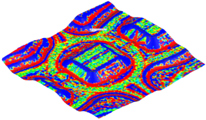
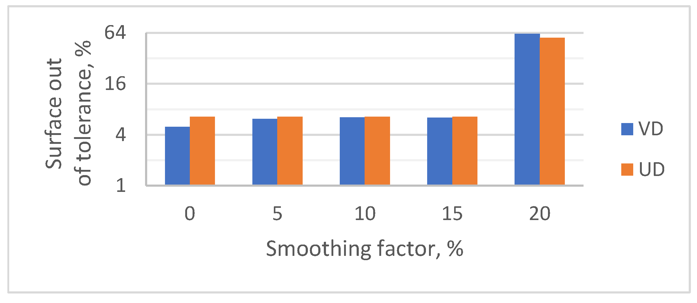
In the case of the analyzed model, it was found that the use of the smoothing function with coefficient values up to 20% did not cause any noticeable changes in the accuracy of surface mapping. Only exceeding this value led to a significant deterioration in the quality of the model, which was manifested by the blurring of topographic details and the deformation of the edges of mesh elements. At the same time, it should be noted that due to the abrupt nature of the change in the smoothing coefficient value, it was impossible to precisely determine the limit value at which the quality of mapping deteriorates.

The observed 20% limit may be due to two overlapping factors. First, it is possible that the smoothing function in the Siemens NX environment contains an internal basic smoothing mechanism that automatically applies a value of about 15%, even when the smoothing factor is set to 0%. This would explain the lack of difference in model quality from 0% to 15%. Second, the geometry of the surface, which consists of a triangle mesh, may have a significant effect. When smoothing factors are too high, above 20%, the blurring of edges between triangular surface elements may exceed their size, leading to undesirable geometric distortions.

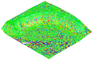
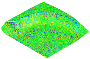
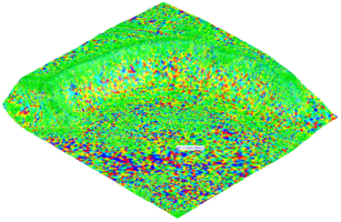
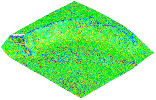
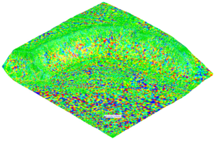
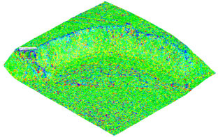
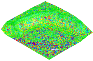
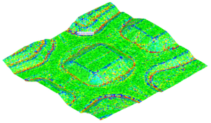
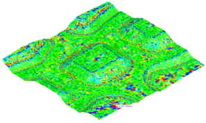
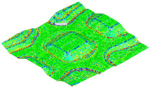
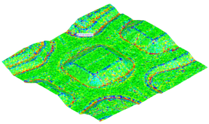
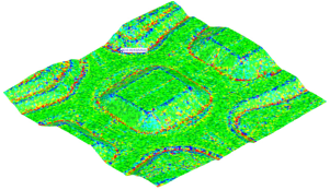
In Figure 4, Figure 5 and Figure 6, it can be seen that within a smoothing factor range of 0–15%, the values of the out-of-tolerance area were similar, regardless of the mesh generation method. A distinct difference was visible only for the VD method at a smoothing factor of 0%, for which the out-of-tolerance area was the lowest among all analyzed cases.

To examine statistical differences between the results obtained for the UD and VD methods and various smoothing factor values, a Student’s t-test for each pair was performed in the statistical program JMP in version 12.0.1. A total of eight groups were compared: four smoothing factor levels × two methods. The significance level was set at 0.05.

The means for all groups, except for the VD method at a smoothing factor of 0%, were statistically equal (p > 0.99). The statistical analysis confirmed that the mean out-of-tolerance area was significantly lower for the VD method at a smoothing factor of 0% than in all other analyzed cases (p < 0.001).

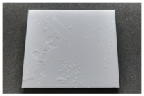
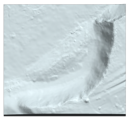
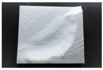
The FDM prints made on the basis of the received data were characterized by low vertical resolution, due to the available T12 nozzle. A large simplification of the surface and low detail was observed, especially for the terrain with a flat morphology. In the case of steep and concave–convex areas, the surface detail was sufficient.

During the research, only the FDM technique was used, and other manufacturing methods were not verified. In order to reflect the obtained results as faithfully as possible, the vertical resolution should be increased by changing the printing technology, for example, to the selective laser sintering (SLS), stereolithography (SLA), digital light processing (DLP), or PolyJet methods, some of which were presented in the literature [5,6]. This recommendation can serve as the basis for further research on the accuracy of mapping terrain topography.

5. Conclusions

The described methodology, which is based on bilinear interpolation and advanced surface creation techniques, allows for the quick and efficient generation of a three-dimensional representation of a terrain surface while maintaining a high level of geometric accuracy.

It has been shown that the use of bilinear interpolation significantly supports the process of creating a surface from a point cloud. The application of a smoothing factor in the range of 0–15% did not cause significant changes in the mean out-of-tolerance area value, regardless of the mesh generation method, and was within the range of 6.0–6.5% out-of-tolerance area. Only in the case of the VD method and a smoothing factor value of 0%, the mean out-of-tolerance area value was lower than all other analyzed means: for the flat surface 5.1%, for the steep surface 5.39% and for the concavo-convex surface 4.96%.In the case of using a smoothing factor of 20%, the percentage of the sample surface area outside the tolerance was at a level of 56.89–80.94%.

Solid models generated on the basis of topographic data can be used, among others, for the physical visualization of terrain structures. An example of their practical application is the creation of tactile models dedicated to blind or visually impaired people, who, thanks to such solutions, can gain access to spatial information through the sense of touch. The use of physical models in special education is an important tool that supports the integration and development of spatial thinking in people with disabilities.

In a broader engineering context, the three-dimensional visualization of the terrain surface can be successfully used for advanced analyses in fields such as civil engineering, geoengineering, or urban planning. These models can be used, among others, for:

• designing technical infrastructure, such as roads, bridges, tunnels, and water reservoirs;
• assessing project feasibility through spatial simulations and collision analyses;
• estimating investment costs based on volumetric modeling and ground mass calculations.

From the point of view of natural and environmental sciences, 3D terrain models are a valuable tool in the analysis of natural phenomena. They can be used, among others, for:

• monitoring changes in the terrain topography related to landslides, erosion, floods, and seismic activity;
• forecasting the effects of extreme weather events;
• developing scenarios for environmental risk management.

In addition, this technology is used in space exploration. Processing data from orbital missions allows for the creation of detailed topographic models of the surfaces of celestial bodies, such as the moon or Mars. These models support the planning of future space missions, both unmanned and manned, thereby facilitating the analysis of possible landing sites, the planning of rover routes, and the testing of technical solutions in conditions close to real ones.