1. Introduction
X5CrNi18-10 belongs to the category of austenitic stainless steels with excellent corrosion resistance in a natural environment [
1]. The excellent properties of X5CrNi18-10 materials come from the essential alloying elements chromium (Cr) and Nickel (Ni). It provides corrosion resistance. In an oxidizing environment, a shielding passive layer is formed. The material’s corrosion-resistant qualities complicate its machining. These steels are considered difficult to machine, have a built-up edge (BUE), and undergo irregular wear during machining operations [
2]. Machining X5CrNi18-10 stainless steel in turning operations is challenging due to high tool wear, increased cutting forces, and difficulties in achieving a good surface finish.
Industrial requirements necessitate achieving a high-precision surface roughness accuracy class, which can be achieved by analyzing surface integrity. The term surface integrity was coined by Michael Field and John F. Kahles in 1964 and has since received growing attention in manufacturing [
3]. It refers to the modified condition of the surface resulting from machining or other surface-generating processes. It is evaluated based on surface roughness parameters, like mechanical strength and metallurgical, chemical, and topological characteristics [
4]. These conditions are examined through hardness variation, residual stress, surface roughness, structural alteration, and corrosion resistance. W. F. Sales et al. [
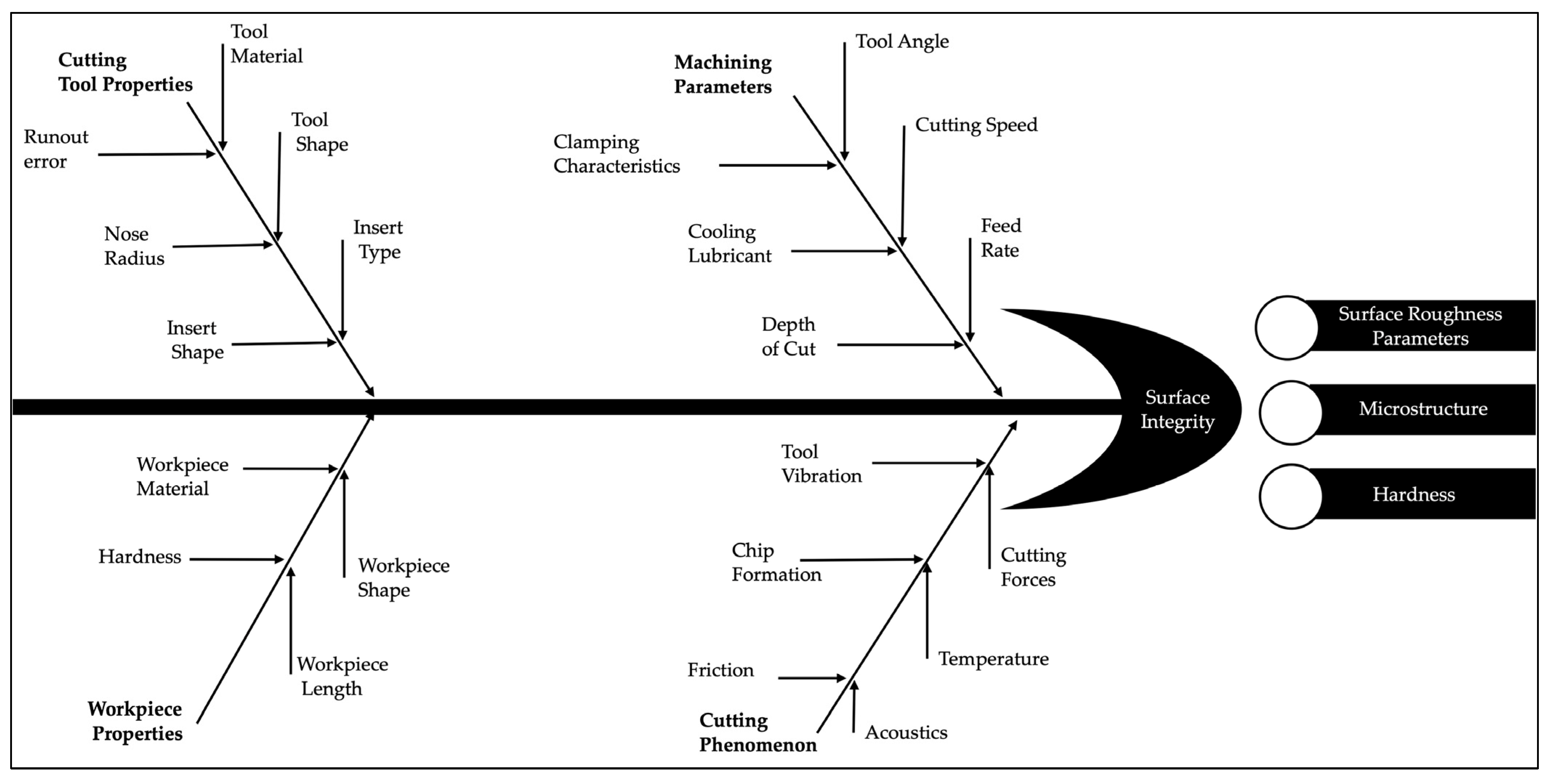
5] found that surface integrity in machining hardened steels is crucial for maintaining fatigue strength and reducing manufacturing costs. However, high temperatures and tool wear can cause surface defects and tool wear. Various factors can affect surface integrity, as represented in the Ishikawa diagram or a Fishbone diagram (
Figure 1). The Fishbone diagram of factors influencing surface integrity is highlighted by many researchers [
6,
7,
8,
9]. These factors affect the surface integrity and the results that constitute the surface integrity.
Paro et al. [
2] used X5CrMnN18-18 stainless steel and highlighted that austenitic stainless steels are difficult to machine. Mishra et al. [
10] showed that EN36C steel has high strength, corrosion resistance, shock resistance, and good fracture toughness properties. However, its machinability is limited by its high strength, corrosion resistance, and high-temperature resistance. The 42CrMo4 material with its chromium content was studied while setting the cutting speed between 100 m/min and 200 m/min. The Core Roughness Depth, Reduced Peak Height, and Reduced Valley Depth were examined and found to be decreased by 2 to 4 times [
11]. Sztankovics et al. [
12] studied the turned surface’s periodic nature and the ground surface’s random nature in 20MnCr5 material. It was found that nearly identical roughness values can be reached in the four procedure versions except for the turning carried out at the highest feed. These studies suggest that the machinability of chromium-nickel alloyed steel requires attention to obtain a good-quality surface and increase efficiency during the machining process. Many researchers [
6,
10,
13,
14,
15] have studied cutting parameters and their effect on the surface roughness parameters of other materials. Thakur et al. [
16] showed that using different grades of nickel-based superalloys decreases surface roughness with increased v
c. Dilsiz M. et al. [
17] developed a high-precision estimation model using a uniform design method. Cutting parameters in nickel alloys containing nickel and chromium were analyzed, and the finding highlights that the parameter that had the most significant impact on surface roughness was the feed rate, which had an effect rate of 35.2%. However, the tool properties and workpiece material can be changed according to industrial and consumer requirements. The main factors that can be controlled during the machining process are cutting parameters like feed rate (f), depth of cut (a
p), and cutting speed (v
c). Increasing demand for X5CrNi18-10 material due to its excellent properties requires a study of cutting parameters and its effects on surface integrity [
18].
This work studies the effects of cutting parameters on surface integrity using Taguchi’s L18 design of experiments (DOE). It highlights the correlation of cutting parameters that affect the surface quality of the machined surface when turning X5CrNi18-10. Analysis of variance (ANOVA) was used to check the regression model’s validity. In addition, this work also presents confocal microscopy, light optical microscopic microstructure, and Vickers microhardness measurement of the turned surfaces to observe the topography, microstructural, and hardness variation due to different cutting parameters on the turned surface.
2. Materials and Methods
X5CrNi18-10 steel, an austenitic chrome nickel steel, is used in the study. This steel’s alloying elements, chromium (Cr) and nickel (Ni), play an essential role due to their unique characteristics. Nickel belongs to the group of austenitic metals. While chromium is ferrite-forming, this steel has an austenitic structure at room temperature with an appropriate amount of Cr and Ni [
19]. The chemical composition of the material with weight percentage is provided in
Table 1. The mechanical properties of the material are mentioned in
Table 2.
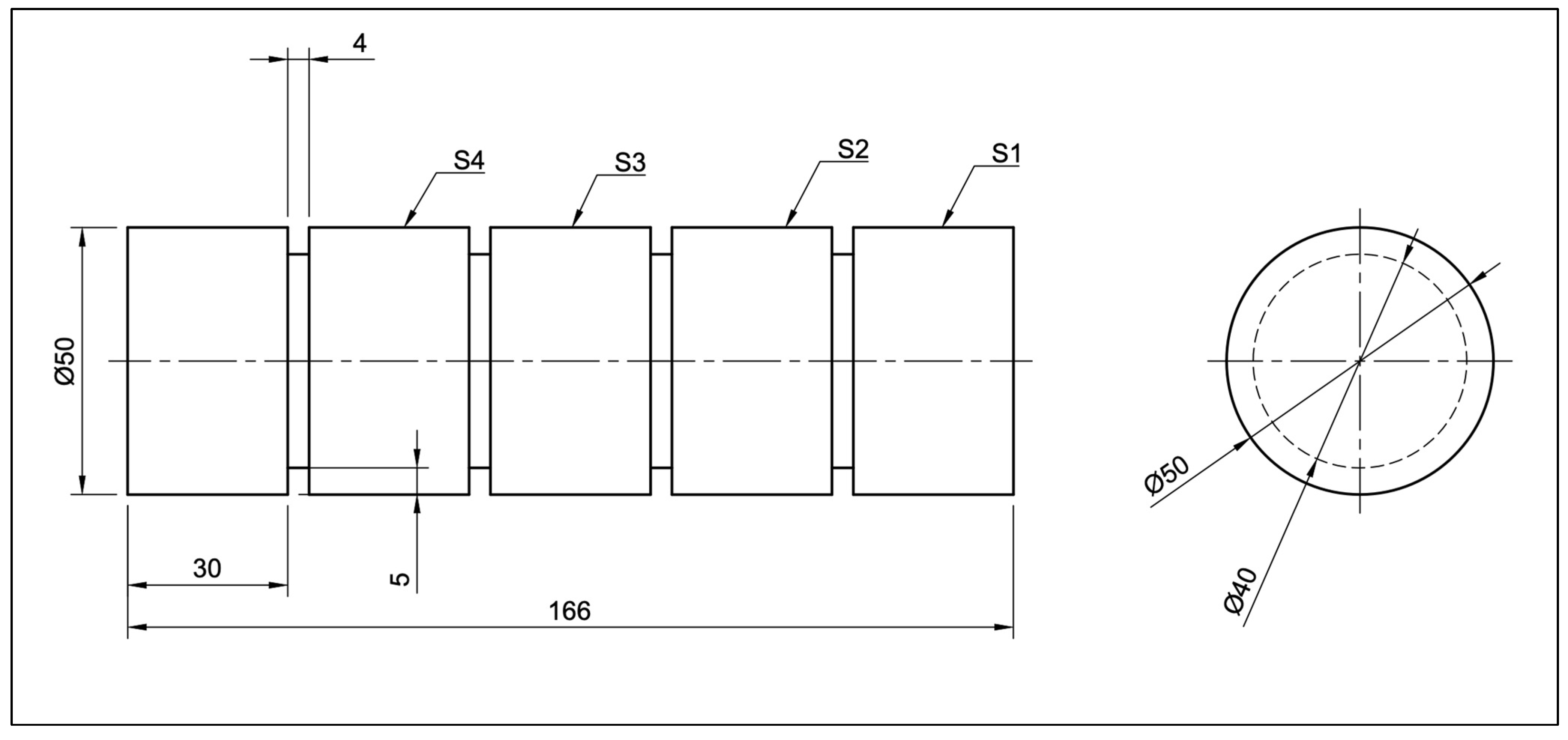
The figure represents a drawing of the workpiece having a diameter of 50 mm. The workpiece had been split into five identical surfaces, each 30 mm in length, with a 4 mm gap groove parting the surfaces with a depth of 5 mm. The surfaces were named S1, S2, S3, and S4. The last part was clamped in the chuck, as shown in
Figure 2.
A total of five workpieces were used in the experiments with eighteen surfaces. The surfaces were partitioned to investigate various cutting parameters, with f, ap, and vc. They were modified based on the Design of Experiments (DOE).
The tool and insert used for the experiment were DDJNL2525M15 and DNMG150604-MF1, respectively, produced by Seco Tools, Björnbacksvägen, Sweden [
22]. The tool and insert are used for all the operations. The insert’s dimensions and form are specified by DN 1506, a particular geometric configuration appropriate for turning operations. The physical vapor deposition (PVD) layer and carbide composition enhance its wear resistance and cutting effectiveness. The insert can be used for both hand orientations as marked neutral. The cutting length of 15.5 mm provides enough space for material removal. It has a thickness of 6.35 mm, which ensures enough strength during the cutting operations. The corner radius is 0.4 mm, indicating the insert is for finishing operation, and the cutting difficulties during the operation will be reduced. The detailed specifications of the tool insert are mentioned in
Table 3.
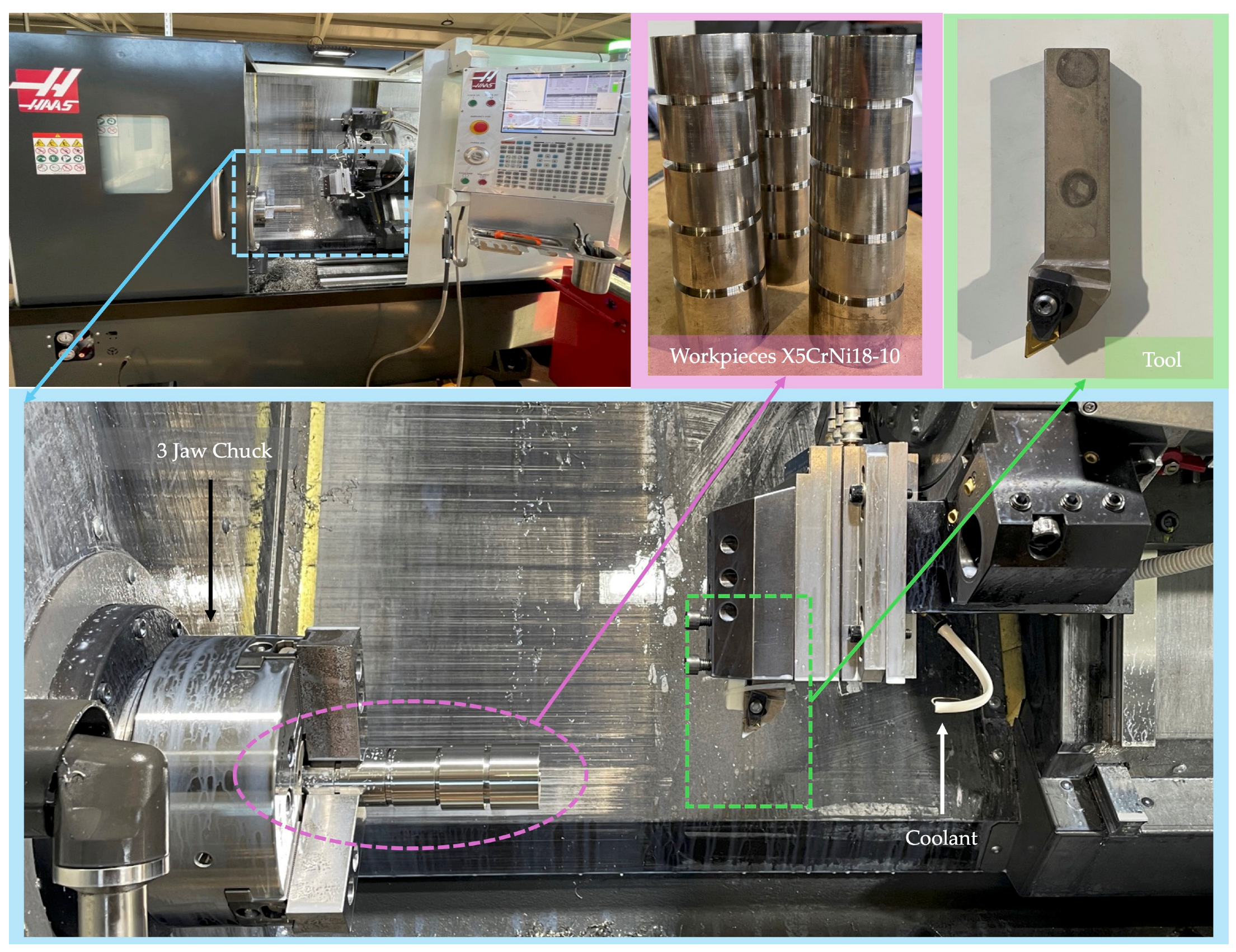
The computer numerical control (CNC) machine used in the experiment is the HAAS series machine, with the serial number ST-20 Y (Haas Automation, Inc, Leoben, Austria). It is a Y-axis CNC turning center, which has a maximum capacity of 298 × 572 mm with a 533 mm swing feature and ±50.8 mm Y-axis travel. It can reach 4000 rpm spindle speed with an A2-6 spindle and a 210 mm chuck. This CNC machine is used for every experiment. All experiments were conducted under wet conditions [
23]. The coolant chosen is a 5% emulsion of CIKS HKF 420 oil type. Coolant is advisable for hardened steel. The outer diameter (OD) turning operation was performed on each surface.
The experimental setup for the CNC machine is represented in
Figure 3. The zoomed-in image of the machine setup is presented in blue, the workpiece in pink, and the tool in green. After the completion of experiments on four surfaces, the workpiece was covered in plastic bags to provide protection, and a new workpiece was inserted in the chuck for machining with different parameters. The setup allowed us to conduct the experiments flawlessly.
Design of Experiments (DOE) methodology predicts and approximates unknown functions for which few values are computed [
24]. There are several methods to design the experiments. To determine the values of v
c, f, and a
p, the 2
k full factorial experimental design method was applied [
11,
25]. Several researchers have found the Taguchi method more efficient in understanding the influence of parameters in machining operations [
26,
27,
28].
According to Taguchi’s concepts, selecting a suitable orthogonal array (OA) depends on the processing parameters’ total degrees of freedom (DOF). With a total DOF of 5 for the experiment, the selected OA must include at least that many degrees of freedom.
Taguchi’s L18 OA was used to design experiments. L18 was chosen because the number of samples provides efficient variation while considering economic and environmental factors. Using multiple levels in each parameter at L9 may raise concerns about accuracy, while L27 can be financially challenging. Therefore, the L18 OA offers the best solution.
Taguchi’s L
18 OA is presented in
Table 4, precisely developed to examine the effects of varied machining variables on the results. The a
p is tested at two steps, 0.5 mm and 1 mm, while the v
c is examined at three rates: 150, 200, and 300 m/min. The f is also changed across three levels: 0.08, 0.16, and 0.24 mm/rev. S1 represents surface number 1 with a
p of 1 mm, v
c of 15 m/min, and f of 0.08 mm/rev. Similarly, the cutting parameters varied for other surfaces.
Table 4 provides sufficient variation in these parameters to evaluate how f, a
p, and cutting velocity affect the surface quality. X5CrNi18-10 is an ISO M-type material grade, and DNMG150604-MF1 CP500 is suitable for machining ISO M-type materials. The initial cutting parameters used in this study, cutting speed (v
c) in m/min, depth of cut (a
p) in mm, and feed rate (f) in mm/rev, were selected based on the manufacturer’s guidelines for DNMG150604 insert. These parameters were then varied at higher and lower levels to analyze their effect on machinability. Cutting speed is vital in machinability due to its impact on cutting forces during material removal. A cutting speed (v
c) of 150 m/min was used to study the effect of low v
c, while 300 m/min was used to evaluate the impact at higher speeds.
This variation helps identify the effects of the manufacturer’s suggested parameters and the impact of the variations on surface parameters in hard turning.
After the completion of the machining operation on all the surfaces, the surface roughness parameters were calculated by AltiMap 6.2 using AltiSurf 520, Altimet SAS, Thonon-les-Bains, France.
The surface 2D profile was measured according to ISO 21920-2 [
29]. A Gaussian filter (λc) was applied following ISO 21920-3 [
30] to reduce the noise. The 2D surface profile was measured for all eighteen machined surfaces, with a sampling length of 10 mm at the scale of 100 μm using a CL2 confocal chromatic sensor. The examined surface roughness parameters are AA Surface Roughness (R
a) and Mean Roughness Depth (R
z). The measurement was repeated three times to achieve higher accuracy during measurements. Surface roughness is measured using arithmetic roughness average (R
a) or arithmetic average surface roughness (R
a). This metric is often called the arithmetic mean roughness value, arithmetic average (AA), or centerline average (CLA). The value of the integral is usually approximated using the trapezoidal rule when evaluated from digital data. R
a denotes the arithmetic average deviation from the mean line (μm), L represents the sampling length, and Y signifies the ordinate of the profile curve [
31].
R
z is the average absolute value of the five highest peaks and the five lowest valleys determined by the sampling length. This measure is usually used to determine whether the profile displays peaks that could influence static or sliding contact effectiveness. The evaluation of R
z is conducted using Equation (2).
Three-dimensional surface topography, which describes surface quality, is studied on the turned surfaces with different cutting parameters, f, a
p, and v
c. The setup parameters for the measurements were chosen according to the ISO 21920-2 [
29] standard.
The study also presents the light microscopic analysis. Microscopic analysis using optical micrographs is essential for the detailed examination of turned surfaces, as it provides insights into surface topography and ensures precision in manufacturing processes. Microscopic surface profiles are necessary for ensuring strict geometric compliances in precision manufacturing [
32]. A light optical microscope, Axio Observer 5, from Carl Zeiss Microscopy GmbH, Jena, Germany, has been used to understand the topography of the turned surface. The optical microscopy setup was connected to the computer, and the scaling was set from the setting to make the image more precise.
The Vickers microhardness tests followed the ISO–6507-1 [
33] standard, using Mitutoyo MVK–H1, a microhardness tester from Mitutoyo Corporation, Sakado, Kawasaki, Japan. Vickers microhardness analysis is essential for examining and understanding the mechanical properties by analyzing the variation on the turned surfaces due to different cutting parameters. Vickers microhardness is correlated with contact hardness and relative contact pressure, which depends on surface roughness parameters [
34]. The study in [
35] used coolant during the turning operation and found that the cooling effect has several advantages on the turned surface. The reduction in depth of the hardened layer in minimum quantity lubricants was noted in comparison to dry cutting, which indicates less structural change. The study in [
36] mentioned that wet cutting decreased the hardened depth of surface integrity. Microhardness testing was performed on the machined surface section with a load of 200 g for a 10 s dwell time. Hardness was measured at three points on each surface, and average hardness was calculated to understand the behavior between cutting parameters and the hardness of the machined surface.
3. Results
Table 5 presents the results of (R
a), (R
z), and Vickers microhardness results.
3.1. Surface Profile Analysis
In surface profile analysis, AA surface roughness (Ra) and mean surface roughness depth (Rz) were studied.
The AA surface roughness value is visualized in
Table 5 and
Figure 4. The AA surface roughness is marked with the blue line in
Figure 4, which shows the surface roughness variation for all 18 surfaces with different cutting parameters. The dark blue stripes represent an f of 0.08 mm/rev, and the light pink stripes represent an f of 0.16 mm/rev. Lightsky-blue color represents an f of 0.24 mm/rev. The orange line marks the mean surface roughness depth.
Figure 4 represents the cutting parameters, with a highlighted cut depth of 0.5 mm and 1 mm on top. The v
c is mentioned for each a
p with 150 m/min, 200 m/min, and 300 m/min, and each v
c is divided into three parts of f.
Figure 4 provides a comprehensive overview of cutting parameters and results of surface roughness parameters, which makes it easy to understand the cutting parameters and how they can influence the surface quality parameters, R
a and R
z.The lowest value of Ra can be seen in surface number 7–1.011 µm with an ap of 0.5 mm, vc of 300 m/min, and f of 0.08. It can be suggested that these parameters can be used to achieve better surface quality in X5CrNi18-10 steel. The highest value of Ra—2.829 µm—is seen in surface number 18 with an ap of 1 mm, vc of 300 m/min, and f of 0.24. It is observable that a change in the cut depth does not influence the results by too much, which suggests that the ap has a very low effect on the surface quality.
Similarly, the mean surface roughness depth (R
z) can be interpreted from
Figure 4. The lowest value of R
z can be seen on surface number 16 and the highest on surface number 9. To achieve good R
z results, low f—0.08 mm/rev, high v
c—300 m/min, and high a
p can be used. However, the change in the a
p does not influence the value of R
z. It can also be observed from
Figure 4 that the dominating parameter that influences the surface quality of X5CrNi18-10 is feed rate.
The lower f provides smooth surfaces, and the higher f increases the value. Also, combining a low f and higher v
c provides smoother surfaces.
Figure 4 represents the detailed analysis of other cutting parameters (f, a
p, v
c) and their effect on the surface roughness parameter in X5CrNi18-10 steel.
The influence of cutting parameters, f, ap, and vc, on the surface profile is studied by Pearson correlation analysis to better understand the results, and it was found in the analysis that f strongly influences the surface roughness. Further, to find the influence of other parameters, estimated marginal means plots were studied.
3.2. Correlation Analysis of Feed Rate, Ra, and Rz
A Pearson correlation analysis was conducted to clarify the link between cutting parameters Ra and Rz. The correlation coefficient ranges from 1 to −1. A correlation coefficient r > 0 indicates a positive correlation between both variables. The r value is approaching +1, which suggests the correlation is strong. A number approaching 0 indicates a weak correlation. If r < 0, a negative correlation exists between the cutting parameters and Ra and Rz, indicating that a change in one variable’s value will not directly influence the other. The fundamental assumptions form the basis of the statistical studies carried out in this work, such as correlation analysis and ANOVA. Correlation analysis implies linearity, while ANOVA implies normality, homogeneity of variances, and independent observations.
The study found a significant strong correlation between feed rate (f), AA surface roughness (R
a), and mean surface roughness depth (R
z).
Table 6 represents the correlation coefficient between feed rate (f) and R
a, which is 0.885, statistically significant at the 0.01 level, suggesting that higher f influences the R
a. The correlation coefficient between feed rate (f) and mean surface roughness depth (R
z) is 0.830, suggesting a high correlation between both variables. It implies that the R
z values also change when the f changes. It indicates an effective positive relationship with linear characteristics, indicating that an increase in f strongly influences the values of R
a and R
z. There is a possibility of less than 1% that this observed connection is caused by random variation. ANOVA is performed between the variables to verify this correlation.
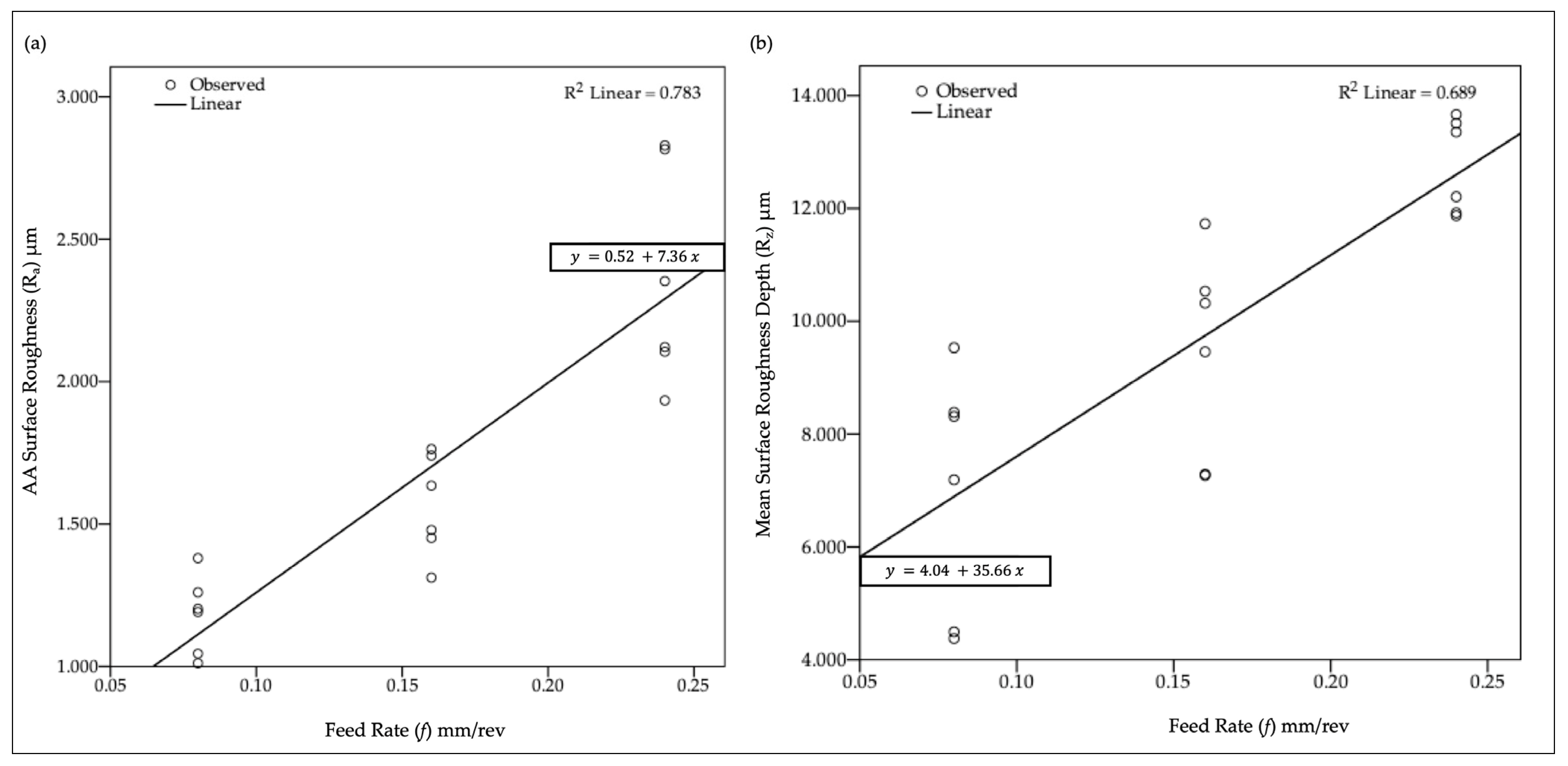
3.2.1. ANOVA of Feed Rate, Ra, and Rz
The regression model acceptability was ensured using ANOVA, and the first-order regression model is developed between f and R
a, shown in
Figure 5a, and is given by Equation (3).
Table 7 represents the ANOVA results, where the dependent variable is AA surface roughness (R
a). The predictor is the constant feed rate (f). “df” in the table represents the degree of freedom. The p-value for this model is 0.000, which suggests that the model is highly significant, with R
2 = 0.783. The R
2 value is very satisfactory.
Figure 5b depicts the linear regression graph for mean surface roughness depth (R
z) and predictor feed rate (f).
Table 8 describes the ANOVA results, where the dependent variable is mean surface roughness depth (R
z), and the predictor is constant feed rate (f).
The predicted outcome is substantial with a
p-value of under 0.05, precisely 0.000. So the effects will be statistically significant, which means high significance. The first-order linear regression model has been developed for feed rate (f) and mean surface roughness depth (R
z), which is given by Equation (4).
with R
2 = 0.689, the R
2 value is very satisfactory.
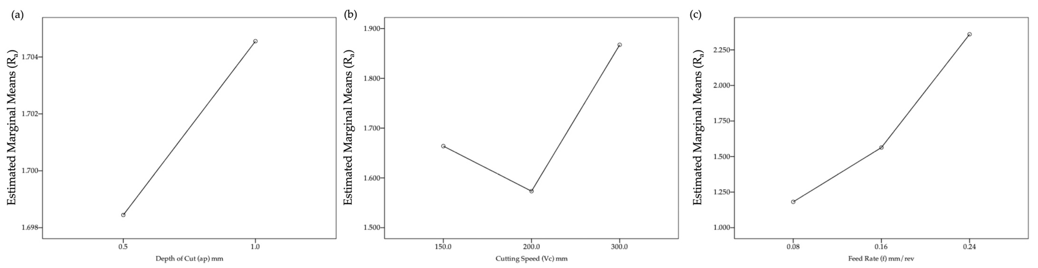
3.2.2. Estimated Marginal Means Plots
The estimated marginal means (EMM) plot helps to understand the influence of a variable and its effects on another variable.
Figure 6 describes the main effect plot between three main cutting parameters, f, a
p, and v
c, and its effects on the R
a variable.
Figure 6a represents the main effect plot between a
p and R
a, and the line represents that with the increase in a
p from 0.5 mm to 1 mm, a slight increase in R
a can be noticed. The depth of the cut is changed at two points. It is critical to change the depth of the cut.
Figure 6b represents the main effect plot between v
c and R
a. The EMM plot suggests that the value of R
a is decreased by changing the low v
c to medium v
c. However, increasing the v
c from medium to high increases the value of R
a. Analyzing the EMM plot suggests that medium v
c provides better results.
Figure 6c represents the EMM between f and R
a with three points, which suggests that by increasing the f, the value of R
a increases, so to achieve better results, f should be kept at a minimum.
Figure 7 represents EMM plots between cutting parameters, depth of cut, v
c, f, and R
z.
Figure 7a represents the main effect plot between a
p and R
z. As a
p increases, the value of R
z decreases, which suggests that with the rise in a
p, the value of R
z decreases.
Figure 7b represents the main effect plot between v
c and R
z, which suggests that by increasing v
c from low to medium, the value of R
z decreases, which shows better surface quality, and if v
c is increased from medium to high, the value of R
z decreases again. Analyzing the plot, it can be suggested that increased v
c provides better results, but the depth of roughness decreases.
Figure 7c represents the main effect plot between f and R
z with three points. The value of R
z also increases by increasing f from low to medium and from medium to high.
Analysis of the main effect plot suggests that if the technological requirement is Rz, to achieve better results, ap should be increased to 1 mm, vc should be increased to 300 m/min, and f should be low. Further, the effects of cutting parameters and their impact on 3D surface topography are investigated.
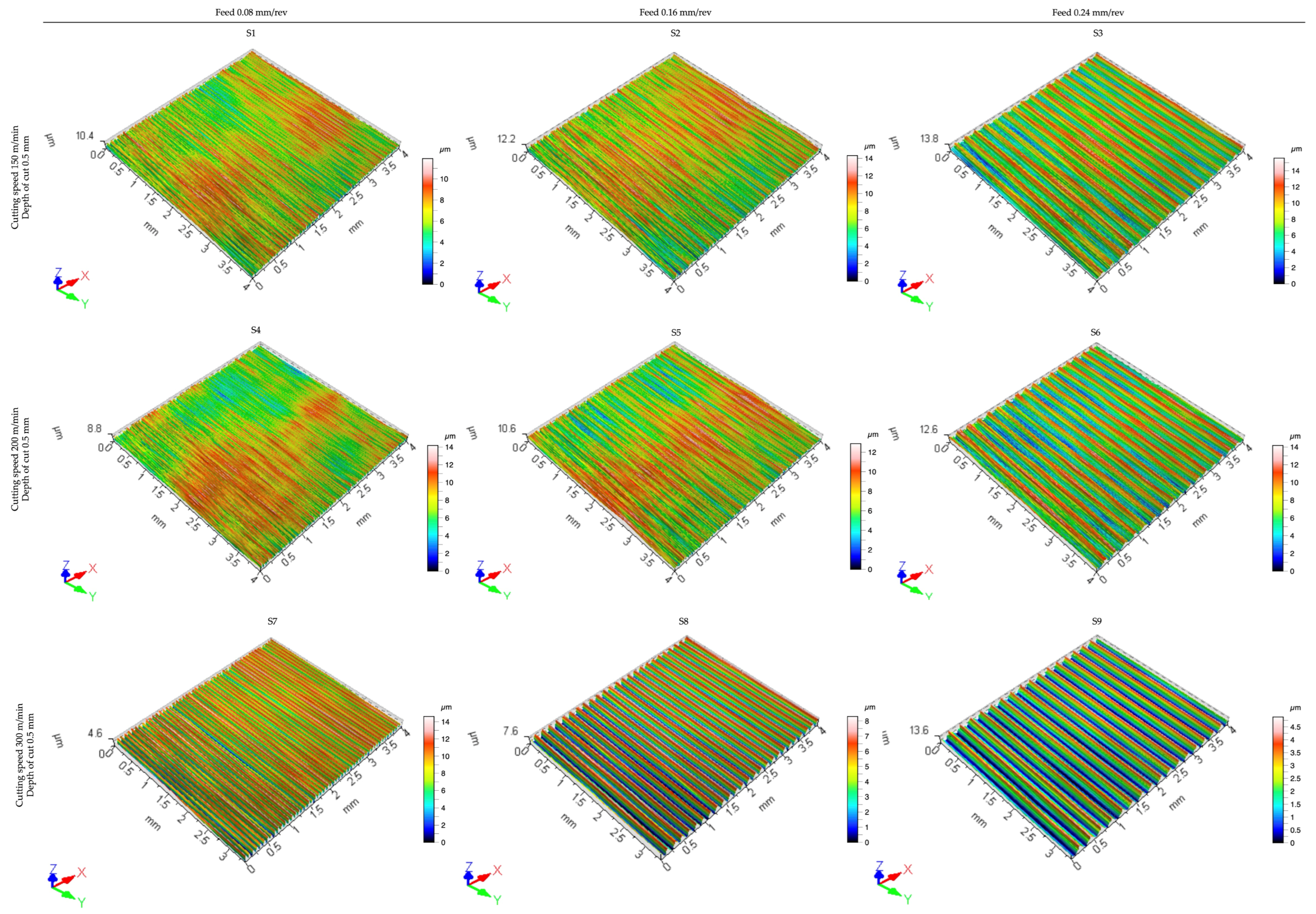
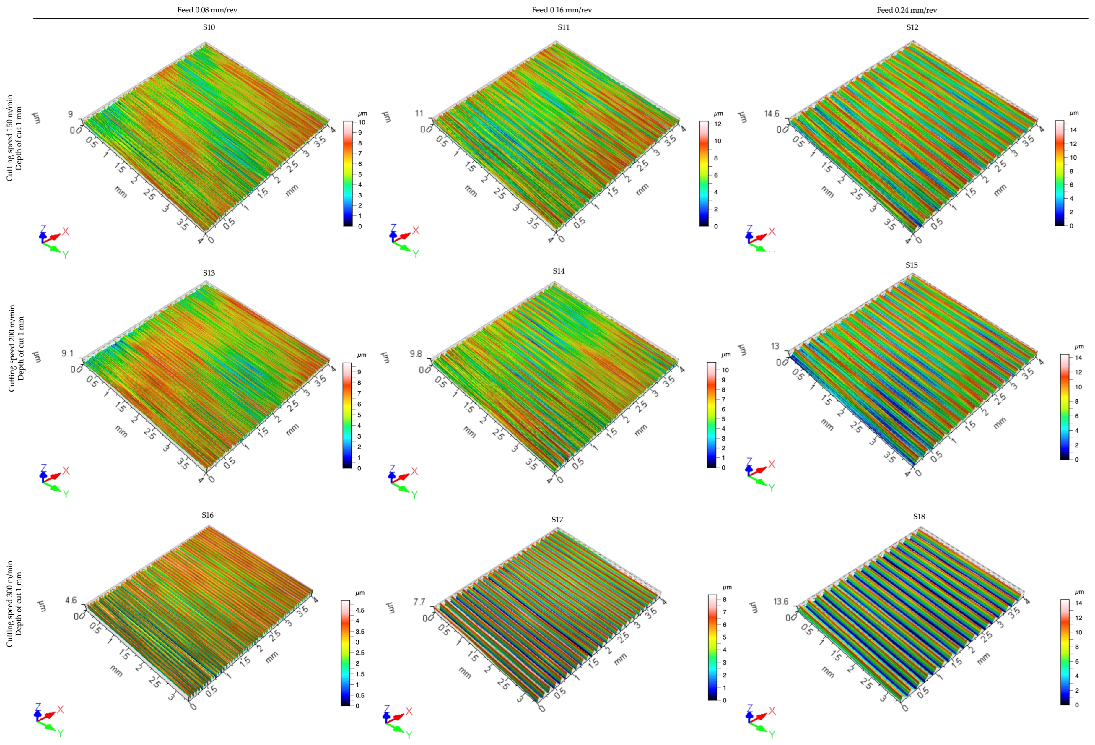
3.3. Surface 3D Topography
The 3D surface topography obtained through confocal microscopy is represented in
Figure 8. A 4 mm × 4 mm area was measured in the X and Y axes, representing the plot (
Figure 8). The z-axis is in micrometers (µm), representing depth at different points. The color gradients in
Figure 8 represent the depth, green and blue areas indicate lower depth or smoother regions, and red areas indicate the peak or rough regions. These variations show the topographical features of the turned surface.
The ap value was 0.5 mm from S1 to S9. S1, with low vc and low f, showing a smoother surface due to minimum material removal per pass, and peaks are less prominent, which is ideal for higher-precision applications. S2, with low vc and medium f, is slightly rougher, as the tool removes more material, and feed marks are more visible due to the higher f. S3, with a low vc and high f, shows a rough surface with visible feed marks, and a high f increases the cutting forces, leading to a higher peak. Surface S4, machined with medium vc and low f, shows a smoother surface than S1, S2, and S3.
The medium vc shows better results in surface quality parameters. S5 with medium vc and medium f shows some feed marks, but no severe defects can be seen. S6, with medium vc and high f, shows feed marks but is slightly improved compared to S3 due to higher vc. With higher vc, S7, S8, and S9 show comparatively rough surfaces. Surfaces S10 to S18 represent the results of low, medium, and high vc and f with a depth of 1 mm cut. S10, with a low vc and low f, shows a smooth surface but is rougher than S1 due to the increased depth of the cut. Increased depth can be seen due to cutting forces. S11, with a low vc and medium f, shows a slightly rougher surface due to increased f. S12 shows a rough surface with low vc, high f, and high ap. A high f increases the cutting forces, which leads to roughness. S13, with a medium vc and low f, shows a smoother surface because of the increased vc. Medium vc provides better results with a low f. S14 with medium vc and medium f shows balanced roughness but is slightly improved. S15, with medium vc and high f, shows a rough surface.
S16, S17, and S18, with high v
c and low, medium, and high f, show rough surfaces. It can be analyzed from topographical images that the depth also increases with a higher f, and medium v
c provides smooth surfaces with an equal distribution of peaks at low a
p. The technological parameters can be chosen based on the requirements. Three surfaces were selected, S4, S5, and S6, based on surface analysis results for further light microscopy analysis. The cutting forces and vibration data for this parameter are presented in [
37].
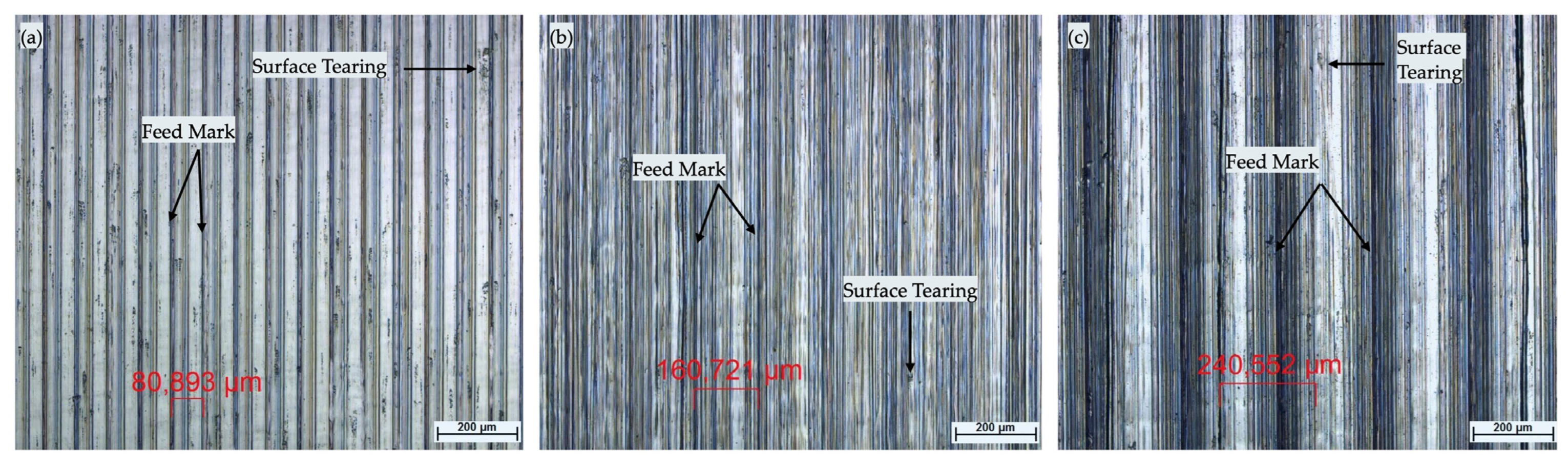
3.4. Microscopic Analysis
Based on correlation analysis and topography results, three surfaces were selected based on f, cutting phenomenon, and surface profile analysis.
Figure 9 represents the optical micrograph of the machined surface numbers 4, 5, and 6 with different fs, 0.5 mm a
p, and 200 m/min v
c.
Figure 9a–c show the results of the spacing of machined surfaces with varying f and feed marks.
Figure 9 highlights the surface tearing at several points that represent the defects in the surface. The machined surface’s strip spacing becomes narrower when the f decreases. During low and high f, the surface tearing can be seen at several points in
Figure 9a,c. With a lower f of 0.08 mm/rev, the surface tearing is high, and minimal surface tearing can be noticed at a medium f. This analysis was only performed for three experiments with the same v
c and the same a
p to analyze the variation in f on the surface defect, which is essential to examine the surface integrity of the machined part.
3.5. Vickers Microhardness Analysis
The analysis provides a non-linear relation.
Figure 10 represents the hardness variation with cutting parameters. Dark blue bars represent the hardness with an f of 0.08 mm/rev, pink bars represent the hardness with an f of 0.16 mm/rev, and sky-blue bars represent the hardness with an f of 0.24 mm/rev. Each f is divided by v
c, and each v
c is separated by a different a
p, as shown in
Figure 10. From
Figure 10 and cutting parameters, it can be concluded that at a low v
c of 150 m/min, the f increases microhardness for both depths of cut (0.5 mm and 1.0 mm). For a medium v
c of 200 m/min, the value of hardness is less consistent, but hardness is increased with an increase in f until 0.16 mm/rev. The effect of high v
c on microhardness is more varied and inconsistent. From surface numbers 1, 2, and 3, it can be observed that with the increase in f, hardness also increases, which can be visible in surface numbers 4 and 5, but it drops at moderate v
c and high f. It can be concluded that a low v
c of 150 m/min with a medium f of 0.16 mm/rev provides better results in terms of hardness.
4. Discussion
The study aimed for an understanding of the impact of machining settings on surface integrity, where the surface roughness parameter or surface finish with correlation analysis of the influencing parameter, surface topography, optical micrograph, and microhardness is analyzed, providing insights to achieve high-precision class accuracy surface finish.
Among all the surfaces, surface number 7 has the lowest value of Ra—1.011 µm, with cutting parameters ap of 0.5 mm, vc of 300 m/min, and f of 0.08. It is recommended to improve the surface quality of X5CrNi18-10 steel. The highest value of Ra is 2.829 µm with ap of 1 mm, vc of 300 m/min, and f of 0.24 in surface number 18. It is observable that changing the depth of the cut does not influence the results significantly. The depth of the cut has minimal impact. Surface roughness analysis results highlight that to achieve the best AA surface roughness (Ra) and mean surface roughness depth (Rz), the given cutting parameters, ap—0.5 mm, vc—300 m/min, f—0.08, should be used.
A strong correlation can be noted between f and Ra, Rz. The coefficient of correlation (r) value between f and Ra is 0.885. The coefficient of correlation (r) value between f and Rz is 0.830. These values are very close to 1, suggesting a very strong correlation. To achieve the best surface quality in X5CrNi18-10, f must be chosen wisely. ANOVA results for both models are highly significant, with a p-value of 0.000. Several limitations must be taken into consideration in ANOVA and correlation analysis. The normality and variance homogeneity assumptions may affect the result’s reliability if not fully satisfied. Future studies could benefit from larger sample sizes.
EMM plot or main effects plots analysis between the cutting parameters ap, vc, f, and Ra, Rz suggests that with the increase in ap from 0.5 mm to 1 mm, a slight increase in Ra can be noticed; however, as ap is increased, the value of Rz decreases. The plot also suggests that by changing vc from low to medium, the value of Ra decreases, which means a smoother surface, and increasing the vc from medium to high increases the value of Ra, which means a rough surface. In terms of Rz, by increasing vc, Rz decreases at both points, so if Rz is the technological requirement, the value of vc must be kept high during the turning operation. The EMM plot also suggests that by increasing f, the value of Ra increases, so f should be kept at a minimum to achieve better results. The combined effect of cutting parameters analyzed for better surface roughness (Ra) suggests that a low ap, medium vc, and low f decrease the Ra value, indicating a smoother surface. However, to decrease the Rz value, a higher ap with a higher vc and a low f is recommended.
Surface 3D topography results suggest that ap is 0.5 mm from S1 to S9, S1 with low vc and low f shows a smoother surface due to minimum material removal, and peaks are less prominent, which is ideal for higher-precision applications. It can be analyzed from topographical images that the depth also increases with a higher f, and medium vc provides smooth surfaces with an equal distribution of peaks at low ap.
Microscopic analysis showed the machined surface spacing at different fs. Surface tearing can be seen for low and high f. To avoid surface tearing during the machining, the f must be medium at 0.16 mm/rev.
Microhardness results suggest that a low vc of 150 m/min increases the microhardness for both depths of cut. The effect of high vc on microhardness is inconsistent.
The cutting forces and vibration data for this study are presented in [
37], where f influences the active vibration and active cutting forces during machining.


