Development of Impact Factors Reverse Analysis Method for Software Complexes’ Support Automation

Abstract

This research represents a corresponding and developed specialized impact factors reverse analysis method for software complexes’ support automation; it is intended for the analysis of impact factors affecting the supported software’s (or processes of its comprehensive support) subjective perception results, as one of the constituent tasks of the more complex problem of software complexes’ support automation. The developed method provides the possibility to restore certain boundaries of impact factors by classifying the multilayer perceptron’s hidden layer neurons and calculating the probability coefficients of the belonging of these neurons to the corresponding specific pre-determined impact factors. The problem of determining the influence of impact factors on the subjective perception of the object of support (the supported software or the processes of its comprehensive support) by the relevant subjects (interacting with this object, providing and implementing its support) was resolved through the approach developed and proposed by the authors in the scope of this research. A key feature of the proposed approach is to assign the neurons of the hidden layers (of the multilayer perceptron type of artificial neural networks) functional–semantic meaning(s), which they have been deprived of a priori, performing (before this) by default an exclusively operational (calculation) function mainly for the correctness of the training and functioning of the multilayer perceptron itself. The potential of the developed method allows us to apply it for solving a huge number of applied practical tasks, such as the one provided in the scope of this research, which is as follows: a practical task of the support team members’ portrait determination, followed by a further search (detection) of the interchangeable members of this support team to ensure the possibility of quick transfer of the stack of tickets (which are in the middle of the active resolution process) between these members.

1. Introduction

Nowadays, the problem of software complexes’ support automation remains one of the urgent scientific and applied problems. One of the main difficulties in solving this problem of software complexes’ support automation is the difference in the resulting vision of the supported object (or process) by the various subjects interacting with it, which, directly or indirectly, participate in the processes of operation and the lifecycle of the supported software complex and influence its comprehensive support accordingly. All these differences in the resulting vision of the supported object (or process) are caused by the presence of various subjective impact factors exerting their influence on both the vision of the software’s support processes and procedures and the vision of the supported software complex itself. Therefore, analysis of these impact factors (with the possibility of their further representation in any form acceptable for automation) is an extremely important and necessary task in solving the more global problem of software complexes’ support automation.

Nowadays, the main (basic or key) directions of automation in the context of a comprehensive support for software complexes (not only a “classic” customer support, but a comprehensive support) are the following:

• Software testing automation;
• Automation of call centers;
• Chatbot automation;
• Automation of service desk requests (both from customers and internally);
• DevOps automation;
• Decision-making automation.

Each of these directions partially (in its own responsibility area) resolves relevant aspects of automation for software complexes’ support. The main task of software testing [1] automation is the replacing of routine, often repeated, clearly structured, and algorithmized activities of people (employees of software testing teams and departments) with appropriate means and automation tools in the form of various scripts, drivers, plugins, modules, and other relevant approaches of software testing automation. The main purpose of call center [2] automation is the opportunity to improve and facilitate the work of people—call center operators—as well as to introduce robotic and/or virtual call center operators that are able to process calls from customers and users fully or partially. The main feature of chatbot [3,4] automation is the possibility of the implementation of the primary communication (with clients and users) function using, for example, natural language processing (NLP) [5] or generative pre-trained transformer (GPT) [6] approaches. The main functions of service desk requests’ automation are, for example, the registration and processing of external requests (tickets) from customer users of client companies [7,8] and various internal requests (tickets) from users within the development companies [9,10], as well as more complex functionality systems—like the one described in [11], which can automatically process crash GitHub logs, analyze them, and register relevant reports—and other similar complex systems. The main task of DevOps [12,13,14] automation is the most effective combination of the software complex’s development stages and is related to this software complex’s stages of IT operations, and the whole of this approach should be manifested in the provision of continuous integration and continuous development (CI/CD) processes [15,16]. The main function of decision-making automation [17,18,19] is providing an auxiliary function for the staff (from regular employee up to middle and higher levels of management personnel) regarding selection and making certain decisions, depending on the input and output parameters, as well as the relevant criteria.

The developed method fills the gap, consisting in the lack of consideration of the subjective perception of the support object (software product) in the context of the represented existing mechanisms of its comprehensive support automation, thereby ensuring additional intellectualization of this automation.

The rest of this paper is structured as follows:

• A literature review is in Section 2;
  A method development, including its three main components, namely a primary generalized model, an algorithm stage, and an appropriate mathematical model, is given in Section 3;
• The main results, obtained as a result of modeling the developed method on a particular example case, resolved from the very beginning to the very end, with a detailed indication of the intermediate results after each separate step of the developed method’s algorithm, including all necessary information about the used means and tools needed for method modeling and approbation, as well as a comparison with the outcomes of the existing similar approaches, are presented and discussed in Section 4;
• The conclusions are in Section 5.

2. Literature Review

The research dynamics of each direction of software complexes’ comprehensive support automation is considered in the current chapter of this paper. For example, nowadays software testing automation is considered to be an absolute norm, mainstream, and even a mandatory common trend. However, not so long ago, according to the data presented in [20], only 26% of all test-cases inside the projects among studied companies were covered with the usage of software testing automation approaches. However, only 10 years later, for example, according to the information presented in [21], there is already software testing automation which is based on the technologies and approaches of artificial intelligence [22], which, in fact, is a transition from the stage of automated software testing to the next phase: fully automatic testing. Unfortunately, in the context of software testing automation, the dominant attention is paid primarily to the automation of technical and technological processes (generalizing and depersonalizing them), which only to a certain extent covers some part of the activities of software testing specialists (or so-called “software testers”), while a significant part of the non-technological aspects of software testing (including impact factors that form a “picture” of the personalized perception of the tested software by each of these specialists, identifying, in such a way, the individuality of this specialist) remains out of consideration and/or is not taken into account.

At the same time, automation is also observed in the first line of software complexes’ customer support represented by call centers, starting from the call routing automation presented in [23] and continuing with the significant achievements in the field of automatic speech recognition presented in [24] and various speech recognition training techniques like the one presented, for example, in [25], as well as various automated assistants similar to the one presented in [26] or automated translators based on the example given in [27]. The main feature of call centers is the communication factor, which plays a dominant role in the context of intersubjective interaction between the support subjects of any researched software complex. At the same time, the represented research (in the context of call center automation) does not pay attention to the impact factors which lead to the subjective perception of the object of communication interaction (which is, in this case, the supported software complex or the processes related to its support) by these subject communicators.

In addition, remarkable results have also been achieved in the field of chatbot automation, starting from agents with modular architecture, as presented in [28], and continuing with systems for constructing the sentential forms similar to the one presented in [29] and the automated voice control systems similar to the one presented in [30]. The research in [31] lists some of the most popular chatbot platforms, such as Siri, Watson, Google Now, and Cortana, which actually have set the mass market mainstream trend for such types of virtual assistants and chatbots with built-in artificial intelligence technologies inside. The research in [32] lists the main methods of chatbot learning, such as DNN, CNN, RNN, LSTM, decision tree, random forest, SVM, and BiLSTM. At the same time, in practice, a lot of users still experience considerable discomfort when interacting with chatbots and continue to prefer “live” communication (in any of its verbal forms) with relevant customer support specialists (which are living people). One of the reasons for such discomfort is, among other things, the lack of analysis of human factors affecting the interaction between subjects—living people—as well as a lack of consideration of the subjective perception of the support object (the supported software complex or the processes related to its support) by each specific individual user while contacting the support service.

Another area of automation during the development and operations of software complexes is automation in the scope of the registration and initial processing of service desk requests, both “external” (driven from outside by the customers) and “internal” (initiated inside the development company). For example, the research in [33] considers the approach of automated sorting and the assignment of requests related to system defects. In the research in [34], the incident categorization automation process is considered, while in the research in [35] and [36], system defect categorization automation approaches are presented, which use latent Dirichlet allocation and fuzzy logic, accordingly. The automated assignment of electronic e-mail requests (tickets) sent by customer users and addressed to the appropriate service support team of the developed software complex, using a set of machine learning methods, is considered in the research in [37]. At the same time, as in previously considered cases of software complexes’ support automation, within the scope of the represented research on the automation of registration and initial processing of service desk requests, there is no relevant analysis of the factor(s) of the subjective perception (by each of these customers’ users) of the object of support, which, in turn, leads to the lack of appropriate corrections necessary to ensure the reliability of information received from these end users.

DevOps automation direction (of comprehensive software support) is also actively developing. One of the most basic and fundamental works in this direction is the research in [38]. A holistic DevOps knowledge management methodology is presented in [39]. According to results presented in the research in [40], 80% of software practitioners (who participated in this research) reported that software building is actually the easiest part of the automation, followed by software packaging and deployment (51.2% and 43.9%, accordingly). The research in [41] additionally emphasizes the importance of DevOps implementation into the development life cycle of each software complex, as well as the fact that DevOps involves not only changes in processes, but also significant changes in the software complexes’ development method(s). CI/CD automation (the combined practice of continuous integration and continuous delivery) is presented in [42] as one of the most essential components of the present DevOps methodology. At the same time, in the scope of the above studies in the context of DevOps automation, there is also no analysis of the factors influencing the subjective perception of the object of automation (the supported software product, as well as the relevant processes for its comprehensive support and related operational processes), which (factors), nevertheless, form both the strategic and tactical vision of these operational processes by each of the subjects, which directly support, provide, perform, and implement these processes.

Simultaneously with all the above-mentioned areas of automation, the direction of decision-making automation is actively developing as well. In particular, the research in [43] presents a proactive support decision-making framework called RADAR, which is based on both research fields of automated planning and artificial intelligence. RADAR helps the decision-making person to achieve his/her goals by providing warnings and suggestions about possible plan flaws and resource constraints. This was achieved by generating and analyzing the benchmarks that any successful plan must meet before achieving the goals. Also, the approach proposed in the RADAR framework is fully consistent with the concept of naturalistic decision making. Another example, which is also probably one of the most popular kinds of automated decision-making usage, is the various smart-systems, such as “smart home”, which is presented in [44]. However, this direction is also actively developing in the field of software development itself and is considered, for example in the research [45], where the approach of real user feedback-based automatic classification of software products’ non-functional requirements is presented, and [46], where the automatic classification of functional and non-functional requirements with the usage of supervised machine learning is presented. The research in [47] represents a comparison of data-driven decision making (DDDM) with automated data-driven model-based decision making (MBDM). In fact, nowadays automated decision-making systems have long left the boundaries of both smart systems and software development and confidently entered the mass market in its various forms. According to the results presented in the research in [48], the European Consumer Organization clearly analyzes the increase in automated decision making, which is based on appropriate algorithms for commercial transactions, and its impact on the functionality of consumer markets and societies. At the same time, the research in [49,50] raises issues caused by the rapidly growing influence of automated decision-making systems and the appropriate challenges and risks caused by these systems. But even despite these risks, interest in these systems continues to grow further; so, they continue to develop and evolve accordingly. In general, decision making is a highly subjectivized process, as each subject (on which the adoption of the relevant decision depends) justifies it in its own personalized way, relying, first of all, on one’s subjective vision and perception of the object of support (the supported software complex or the processes related to its support), which (this subjective vision) is shaped by relevant impact factors that, unfortunately, are also not taken into account in the context of the represented studies and research carried out in this direction of decision-making automation in the context of software complexes’ support automation.

So, as we can see from the conducted review and analysis, automation has already deeply penetrated inside all key stages of the software complexes’ development and operation—starting with their testing and ending with automatic analysis of real feedback left by users (living people) of these software complexes.

Unfortunately, lack of attention to the subjectivization of the support object’s (supported software products or processes related to their comprehensive support) perception is a common problem (gap) in all the reviewed and presented research given above, which is aimed at automation of the component processes of the software products’ life cycle. In turn, this leads to a depreciation of the impact of the subjectivization of the comprehensive support objects’ perception by those subjects (e.g., personnel) who directly implement and provide such comprehensive support fully or particularly.

That is why, within the scope of the current research, a more global approach for the study of software complexes’ comprehensive support automation is proposed by the authors: in this research we actually raise up to the next (higher) level, which connects all the described manifestations of automation—from testing to decision making. And at this next higher level, we are mainly interested in the problem of various impact factors having an influence on the representation results of the supported software complexes (or processes) by all the appropriate participants (subjects of interaction) of this support—starting from the testers, continuing with the customer (and/or product) support specialists, and ending with real users at the customer(s) side. Undoubtedly, each of these subjects, directly or indirectly interacting with the supported software complexes, consciously or subconsciously comes across a set of both universal and individual impact factors, which, one way or another, at different degrees of influence, definitely affects their subjective resulting perception of this supported software complex or its support processes. That is why (in context of this research) we are so interested in these impact factors and the possibility of their further research, analysis, differentiation, calculation, and quantitative assessment, as well as the determination of the degrees, levels, and limits of their influence, etc.

Therefore, the main goal of this research is to develop an impact factors reverse analysis method for software complexes’ support automation; it is based on a specially developed algorithm, as well as the appropriate mathematics, software, and additional required models and components presented in this research.

3. Method Development

The developed method consists of three main components, namely:

• Primary generalized model;
• Algorithm stages;
• Mathematical model.

The main purpose of the developed and proposed primary generalized model is to provide a simple, understandable, and at the same time universal way of formalizing the representation of the support objects’ perception subjectivization.

The main purpose of the developed and proposed algorithm stages is to provide a clear algorithm to enable further automation and software implementation (coding), as well as computer modeling of the developed method.

The main purpose of the developed and proposed mathematical model is to ensure a fundamental mathematical basis for the developed method, which will provide additional opportunities both for mathematical modeling (as an integral part of computer modeling and programming) and for the further use of all existing mathematical tools in order to obtain any proposed, necessary, possible improvements and/or modifications.

Let us start from the consideration that any supported software complex has a number of input characteristics I1…In, as well as a number of output characteristics (as a result of its subjective representation) O1…Om (where “m” does not necessarily have to be equal to “n”). Input characteristics are the characteristics which are close (as much as possible) to the objective (real or true) ones, while the output characteristics are the results of the subjective perception of the supported software complex (or its support processes) by appropriate subject(s) directly or indirectly interacting with this supported software complex.

In ideal (“vacuum”) conditions, those output characteristics are considered as the results of some previously determined and known referential functional dependence from the input characteristics, without any distortions.

However, in real conditions, each input characteristic undergoes certain distortions and “deformations”, and, as a result, all of them are transformed into the corresponding resulting (subjective) output characteristics, which form the final perceptional subjective resulting interpretation of the supported software complex (or processes of its support) by the appropriate subject(s) interacting with it. That is why, finally, each subject of interaction with the supported software complex perceives it in its own individualistic (personalized) way/manner.

The main levers of influence (or tools of deformation) in this process of transformation of the input characteristics into output results are the impact factors. There could be any number (and variety) of them, and each of these impact factors affects each input characteristic of the supported software complex (or the processes of its comprehensive support) in its own way.

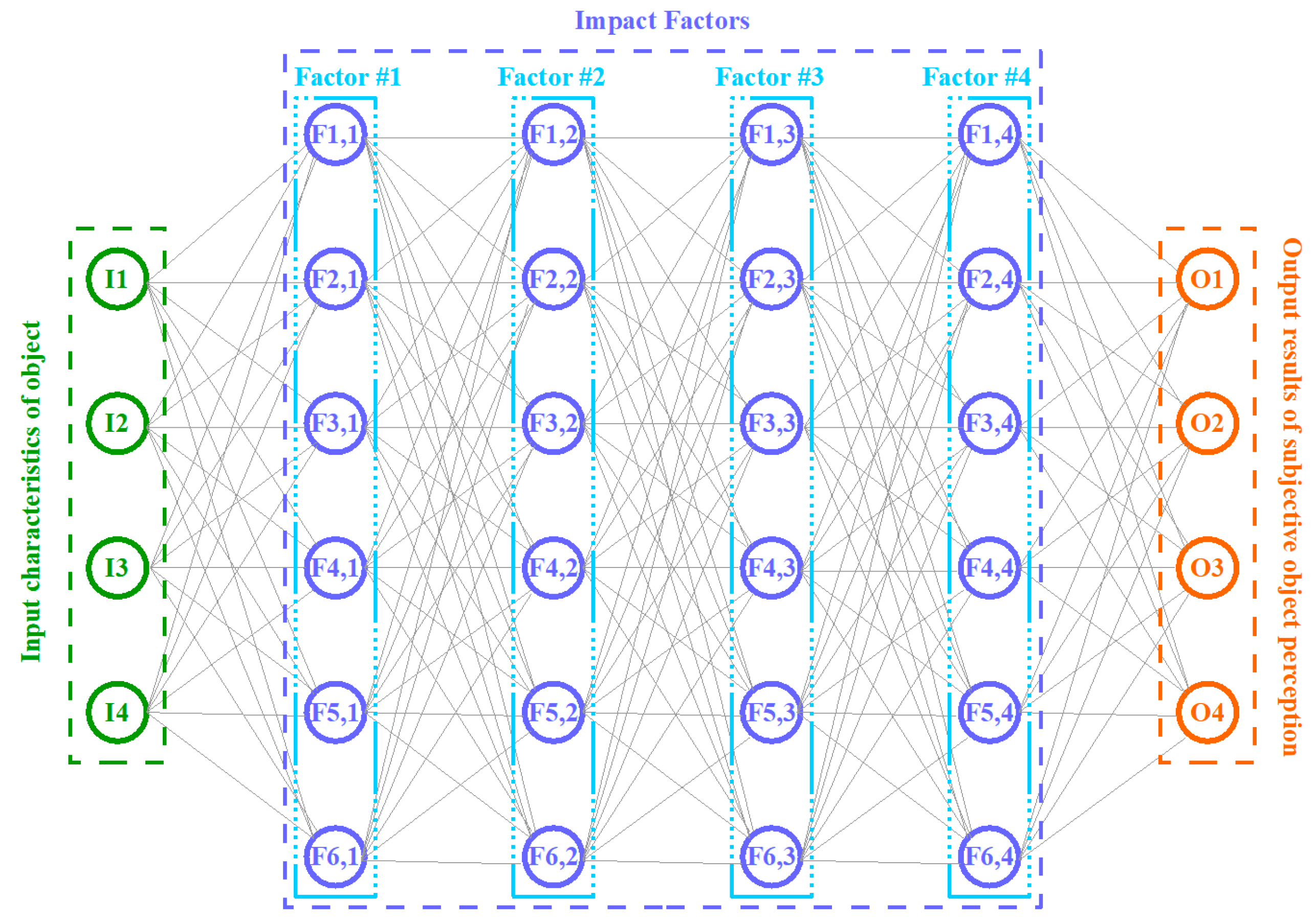
3.1. Primary Generalized Model

The above-described process can be simply interpreted by the developed and proposed (in the scope of this research) primary generalized model of the supported object’s subjective perception, a visualized example of which is provided below in Figure 1.

Depending on the set goals and objectives, the “supported object” could be represented by the supported software complex itself, as well as the processes of its comprehensive support.

According to the developed and proposed generalized model (of the supported object’s subjective perception) each researched supported object should have the following:

• A set of input characteristics;
• A set of sequential impact factors, each of which can influence each of the input characteristics (many-to-many relationship) correspondingly in its own way, gradually (or cascadingly) transforming them into a relevant set of resulting output characteristics;
• A set of resulting output characteristics.

As can be seen in the given graphic representation provided below in Figure 1, the proposed primary generalized model visually reminds the well-known multilayer perceptron (MP), where

• A set of input characteristics is the MP input layer’s neurons;
• A set of impact factors is the MP hidden layers’ neurons;
• A set of resulting output characteristics is the MP output layer’s neurons (with the results of the MP’s operation).

However, the multilayer perceptron in its primary basic concept does not assume the presence of any meaningful or cognitive values for hidden layers’ neurons. According to the well-known classical concept of a multilayer perceptron, all the hidden layers’ neurons (inside any multilayer perceptron) are needed only for purely mathematical calculations and the corresponding training function of the MP. Therefore, it cannot just be assumed that each hidden layer of neurons (in the corresponding constructed multilayer perceptron model) is a separate impact factor, because the structure of a multilayer perceptron itself does not meet such comprehension. Thus, each time when appropriate multilayer perceptron models are implemented for proposed primary generalized models (of the supported object’s subjective perception), the boundaries of the impact factors (presented in these primary models) are actually lost (or blurred) in the appropriate MP models.

So, this is actually the problem which should be resolved, and that is actually why we are so interested in the possibility of identifying (or restoring) these certain lost boundaries of the impact factors influencing the supported object(s) while implementing and using the corresponding constructed multilayer perceptron models for them.

Thus, the main goal of this research is the investigation of the possibility of introducing additional meaningful (or cognitive) values (labels) for the neurons of the hidden layers of the corresponding constructed multilayer perceptron models, in accordance with the determined impact factors of the researched supported object(s).

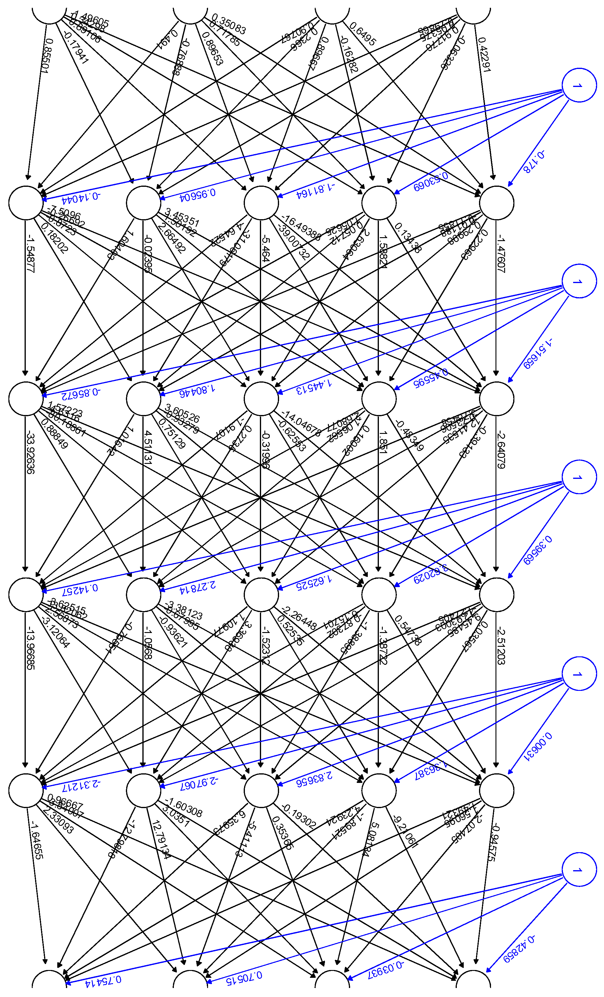
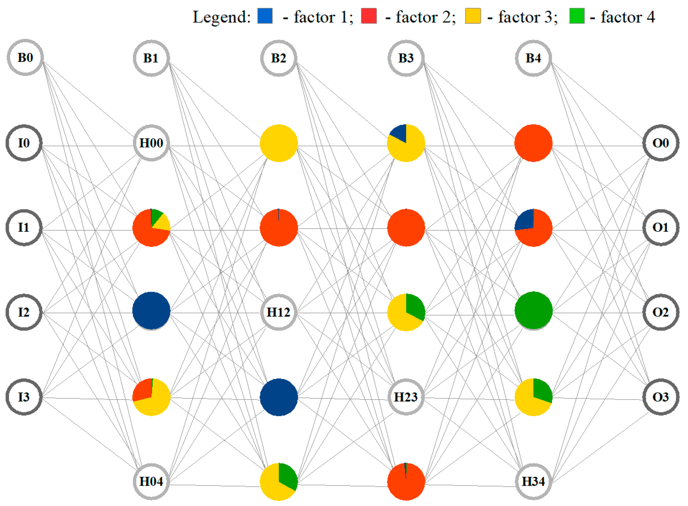
Figure 2 below describes an example of an appropriate multilayer perceptron model corresponding to the primary generalized model of the supported object’s subjective perception (which was already provided in Figure 1 above).

As presented in Figure 2, the corresponding multilayer perceptron model is an example of a real model, one of those which have been used for modeling while working on the issue(s) investigated by authors in the scope of this research. Thus, for better clarity and understanding, all further scientific and practical materials, as well as the investigation results, presented in this research are linked to this particular specific research example (in order to ensure the possibility of tracking the entire research chain, from its very beginning to its complete end).

Therefore, the corresponding developed model of the multilayer perceptron, as described in Figure 2, consists of the following:

• Input layer neurons І0–І3;
• Four hidden layers of neurons (five neurons on each hidden layer, + an additional one bias neuron on each hidden layer);
• Output layer neurons О0–О3.

3.2. Algorithm Stages

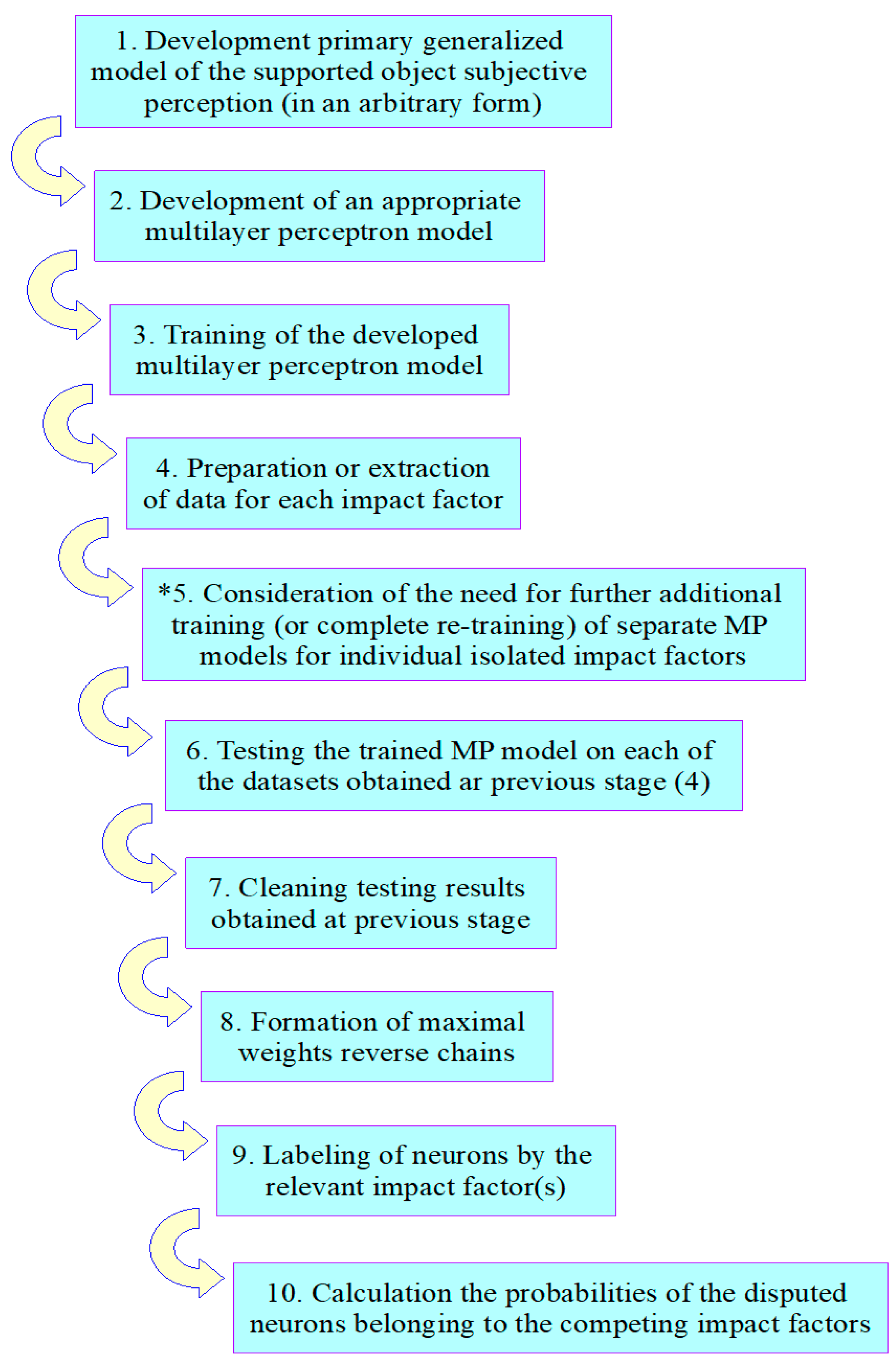
Let us move on to a consideration of the corresponding developed algorithm (and its stages) of the impact factors reverse analysis method for the software complexes’ comprehensive support automation.

The very initial stages of the developed impact factors reverse analysis method are as follows:

Stage 1. Development of a primary generalized model of the supported object’s subjective perception (in an arbitrary form but necessarily including strict indication(s) for all input characteristics and output resulting characteristics, as well as all impact factors).

Stage 2. Development of an appropriate multilayer perceptron model fully corresponding to the previously developed primary generalized model of the supported object’s subjective perception. At this stage, an extremely important and mandatory requirement is ensuring a unique relationship between each impact factor and the corresponding hidden layer(s) of the multilayer perceptron (in the case that their relationship type is different, it is just “one-to-one”).

Stage 3. Training of the developed multilayer perceptron model, performed on a relevant, appropriately prepared, training dataset(s).

For better understanding, Figure 3 below additionally provides appropriate graphical representation of the full process described in all the provided stages of the developed algorithm.

The next stages are the main stages for the analysis of all the defined impact factors present in supported object’s subjective perception model, namely:

Stage 4. Preparation or extraction of data for each individual isolated impact factor.

The ideal conditions for this stage (4) are the following:

• The absolute impact of only one (currently considered/investigated) impact factor;
• The zero-level impact of the rest of the impact factors (except the one currently considered/investigated);
• An absolutely clear understanding of how each individual impact factor affects the model in isolation (without the influence of the rest of the impact factors);
• Insight into what will be the input and output data of the model under the isolated influence of only one individual (currently considered/investigated) impact factor.

* Stage 5 (which is an optional stage). Consideration of the need for further additional training (or complete re-training) of separate MP model(s) for individual isolated impact factors. However, this stage (5) is extremely time-consuming, complex, and resource-consuming, and requires a separate consideration (perhaps in separate dedicated research). Therefore, in this research, we use a slightly different approach, which involves using the multilayer perceptron model, already previously obtained in stage 3.

Stage 6. Testing of the trained MP model on each of the datasets obtained in the previous stage (4) for each separate impact factor(s).

Stage 7. Cleaning obtained testing results—as we are only interested in the correct results, while incorrect ones should just be discarded.

Stage 8. In this stage, the corresponding maximal weight reverse chains are built based on each testing result from the previous stage. Each reverse chain is built starting from the correct active MP output layer’s neuron, back through all the MP’s hidden layers, and finalizing at the corresponding MP input layer’s neuron).

Stage 9. Labeling of each of the neurons for each of the reverse chains (obtained in previous stage) in accordance with their belonging to the currently considered/investigated specific impact factor.

Stage 10. Calculation of the probabilities for all neurons (obtained in the previous stage) regarding their belonging to those impact factors to which they have been appropriately labeled in the previous stage. * Here, in this stage, it is also important to understand one important thing—the same neuron can simultaneously belong to the reverse chains of several different impact factors (and such a situation is quite normal). Therefore, the main task of this stage is to calculate the probabilities by which each such specific neuron belongs to each of its impact factors. For such neurons, a separate term is proposed and introduced for the developed method in the scope of this research: “disputed neurons”. And for such impact factors that include disputed neurons, the developed method also proposes and introduces a corresponding separate term: “competing impact factors”.

This stage actually finalizes the description of the developed algorithm.

3.3. Mathematical Model

So, let us move on to the detailed consideration of the developed mathematical component (model) of the impact factors reverse analysis method, according to which the calculation of probabilities (of neurons belonging to the relevant impact factors) is performed in several steps, as provided below. In the first step, the percentage ratio is calculated for the frequency of occurrence of each unique reverse chain (within their impact factors) relative to the total number of all cases (within their impact factors). The appropriate calculations for this first step are performed using the expression given below:

$${\mathrm{FoA}}_{\mathrm{local}}\left[i\right]\left[j\right]={\displaystyle \frac{\mathrm{count}(\mathrm{URC}\left[j\right]\in F\left[i\right])}{\mathrm{count}(\mathrm{URC}\left[\mathrm{all}\right]\in F\left[i\right])}},$$

(1)

where FoA_local[i][j]—frequency of appearance of the [j]-th unique reverse chain within [i]-th impact factor; count(URC[j]$\in$F[i])—the number of appearances of the [j]-th unique reverse chain (URC) within the [i]-th impact factor; count(URC[all]$\in$F[i])—the total number of appearances of all unique reverse chains existing within the [i]-th impact factor.

In the second step, the percentage ratio is calculated for the frequency of occurrence of each unique reverse chain (beyond its impact factors or, in other words, in the general set of cases, a “global dataset”) relative to the total number of all cases (within this general set of cases or the same “global dataset”). Appropriate calculations for this second step are performed using the expression given below:

$${\mathrm{FoA}}_{\mathrm{global}}\left[i\right]\left[j\right]={\mathrm{FoA}}_{\mathrm{local}}\left[i\right]\left[j\right]\cdot \mathrm{FI}\left[i\right],$$

(2)

where FoA_global[i][j]—the frequency of appearance of the [j]-th unique reverse chain of the [i]-th impact factor within the global dataset; FI[i]—index of the [i]-th impact factor (factor index—FI).

In turn, the impact factor index is calculated using the following expression provided below:

$$\mathrm{FI}\left[i\right]={\displaystyle \frac{\mathrm{count}(F\left[i\right]\in \left[\mathrm{General}\right])}{\mathrm{count}(F\left[\mathrm{all}\right]\in \left[\mathrm{General}\right])}},$$

(3)

where count(F[i]$\in$[General])—the number of appearances of the [i]-th impact factor within the global dataset; count(F[all]$\in$[General])—the total amount of all cases (for all impact factors) of the same global dataset.

In the third step, the values of the probabilities that the disputed neurons belong to the appropriate competing impact factors are calculated by the following expression:

$$\mathrm{PoDNbtCIF}\left[i\right]\left[k\right]={\displaystyle \frac{\sum {\mathrm{FoA}}_{\mathrm{global}}\left[i\right]\left[j\right](\mathrm{Neuron}\left[k\right]\in \mathrm{URC}\left[j\right])}{\sum {\mathrm{FoA}}_{\mathrm{global}}\left[i\right]\left[j\right](\mathrm{Neuron}\left[k\right]\in \mathrm{URC}\left[\mathrm{all}\right])}},$$

(4)

where PoDNbtCIF[i][k]—probability that the disputed neuron [k] belongs to the competing impact factor [i]; FoA_global[i][j](Neuron[k]$\in$URC[j])—the frequency of appearance of the [j]-th unique reverse chain of the [i]-th impact factor within the global dataset (for those unique URC[j] reverse chains which include the disputed neuron Neuron[k]); FoA_global[i][j](Neuron[k]$\in$URC[all])—the frequency of appearance of the [j]-th unique reverse chain of the [i]-th impact factor within the global dataset (for all unique reverse chains of all impact factors, e.g., URC[all], which includes the disputed neuron Neuron[k]).

Therefore, in a global sense, the essence of the concept of the developed (provided above) expressions, representing the appropriate mathematical component/model of the impact factors reverse analysis method, is the following:

• First—the probability of the appearance of each unique reverse chain (with its binding to each of the relevant impact factors, of course) in the global dataset should be estimated;
• then—the probability of the appearance of each disputed neuron (in the scope of each unique reverse chain, to which this neuron belongs, and with the binding of each of these chains to the related impact factor) is estimated, and this provides a specific link between this particular disputed neuron and that particular competing impact factor.

Or, in other words (for some additional, or maybe better, understanding), we have a list of neurons (all of them, including disputed ones) and a list of unique reverse chains (which include these disputed neurons), and these unique reverse chains, in turn, are also part of the impact factors (all of them, including competing ones).

So, we could

• Simply count the number of unique reverse chains (which include some currently investigated disputed neurons) of one single specific impact factor (to which these unique reverse chains belong);
• Then divide this number by the total number of all unique reverse chains (which includes this currently investigated disputed neuron), regardless of the binding of these unique reverse chains to a specific impact factor, but instead just considering absolutely all unique reverse chains (which include this currently investigated disputed neuron) for all impact factors.

However, such an approach will be correct only if

• The probability of the appearance of each impact factor in the global dataset is equal for all impact factors;
• The probability of the appearance of each unique reverse chain in the global dataset is equal for all unique reverse chains.

But the real situation in practice is completely different, and there are specific numerical values of both the probabilities of the appearance of each impact factor in the global dataset and the probabilities of the appearance of each unique reverse chain in the same global dataset.

That is why when calculating the ratio

• of the number of unique reverse chains (which include the currently investigated neuron) of one single specific impact factor (to which these unique reverse chains belong)
• to the total number of all unique reverse chains (which include this currently investigated neuron) for all impact factors

we already take into account such pre-calculated numerical values as

• the probability of the appearance of each impact factor in the global dataset,
• as well as the probabilities of the appearance of each unique reverse chain in the same global dataset.

That is actually what all these developed and provided expressions, representing the appropriate mathematical component/model of the developed impact factors reverse analysis method, really mean.

4. Results and Discussion

This section of the paper intends to present the developed method in as much detail as possible through its practical step-by-step use in a particular example study case.

In addition, for better understanding, this section is structured into subsections, as follows:

• Section 4.1. Working with the developed multilayer perceptron model;
• Section 4.2. Formation of maximal weight reverse chains with the following labeling of neurons by the relevant impact factor(s);
• Section 4.3. Calculating the probabilities of the disputed neurons belonging to the competing impact factors;
• Section 4.4. Example of a practical task resolution by the developed method;
• Section 4.5. Comparison with outcomes of existing similar approaches.

Let us move forward with each of the subsections of the current section.

4.1. Working with the Developed Multilayer Perceptron Model

Thus, the appropriate multilayer perceptron model (for the researched experimental model, presented in this research as an example case) was developed and trained in the R 3.6.3 environment using the “neuralnet” package and the LeakyReLu activation function.

The example code of the corresponding developed software (for this part of the investigation) in the “R” programming language is given below in

Table 1. The code of the corresponding developed software in the R programming language.

support <- read.csv(“:/dataset.csv”) str(support) support_train <- support[1:1000,] support_test <- support[1001:1100,] library(neuralnet) leakyrelu <- function(x) {ifelse(x < 0, 0.01*x, x)} support_model <- neuralnet(O1 + O2 + O3 + O4 ~ I1 + I2 + I3 + I4,     data = support_train,     hidden = c(5,5,5,5),     #using default algorithm “rprop+”     act.fct = leakyrelu,     linear.output = FALSE,     threshold = 1, stepmax = 1,000,000) plot(support_model) support_model$weights

:

As the input data for the training and testing of the developed multilayer perceptron model, data from a CSV-file are used (just as an example presented in this paper, because the developed method itself does not set any limitations regarding data representation formats). Before that, all these data (present in this CSV-file) were obtained as a result of the execution of additional software developed in the Python 3.12 programming language using the Thonny 4.1.4 IDE, which was used as a data generation engine. At the same time, all these data in the CSV-file were additionally depersonalized (in particular, they were deprived of any personalization, sensitivity, or semantic load; instead, only “pure numbers” were left) and normalized (input neuron values: [0.1–0.9]; output neuron values: 0 or 1, where only one of four output neurons can be 1, while the rest must be 0). Depersonalization and normalization of these data were also performed by additional software developed in Python. An example of the data from a CSV-file is shown in Figure 4 below.

The accuracy of the developed MP model trained on the testing dataset was achieved and reached up to 96.04%; it could even grow more, but it was specifically decided to not train the model above this level, because for most real cases such accuracy is rarely achieved. So, the main goal was just to make sure that the developed MP model was well trained and could show acceptable, really good, and pretty accurate testing results.

Returning back to our example, in Figure 2 an appropriate trained multilayer perceptron model was obtained corresponding to the primary generalized model of the supported object’s subjective perception. That is, in fact, completed in stage 3 of the developed algorithm for the impact factors reverse analysis method.

So, the next stage (4) is actually a preparation (or extraction) of the data for each individual isolated impact factor. In this stage, each of the impact factors is considered in isolation; so, here we must clearly realize and understand what input and output data of the model we will obtain when isolating the influence (performed on our supported software complex or the processes of its support) of each individual impact factor taken from the set of all available impact factors. At the same time, the influence of all remaining impact factors (except the single currently investigated factor) must be reduced to zero (0).

For example, in our specific example case, presented in this research, an appropriate strategy was chosen, according to which each separately taken impact factor (out of four existing in our example model) is responsible for activation of only one specific resulting output neuron (out of four existing in our MP model). (* But this is just an example; in other cases, the strategies of the isolated influence of the impact factors could be completely different; however, we consider such a specific example primarily for better simplicity, clarity, and understanding of the whole of the material represented in this research as an example).

By means of appropriate additional developed Python software, the corresponding CSV-files were prepared with data for testing the isolated influence of each individual impact factor of the developed and considered example model.

The next stage (6) is responsible for the testing of the trained MP model on each of the datasets obtained in the previous stage (4) for each separate impact factor(s). In other words, it means that we should use the datasets from each separate prepared CSV-file (for each separate corresponding individual isolated impact factor) for testing the same trained multilayer perceptron model obtained in stage (3).

In the next stage (7), the results (obtained in the previous stage of testing for each individual isolated impact factor) should be cleared, leaving only the correct results; that is, those where (at the output of our multilayer perceptron model) we obtained the actual correct result which fully corresponded with the expected result present in the appropriate CSV-file.

4.2. Formation of Maximal Weight Reverse Chains with Following Labeling of Neurons by the Relevant Impact Factor(s)

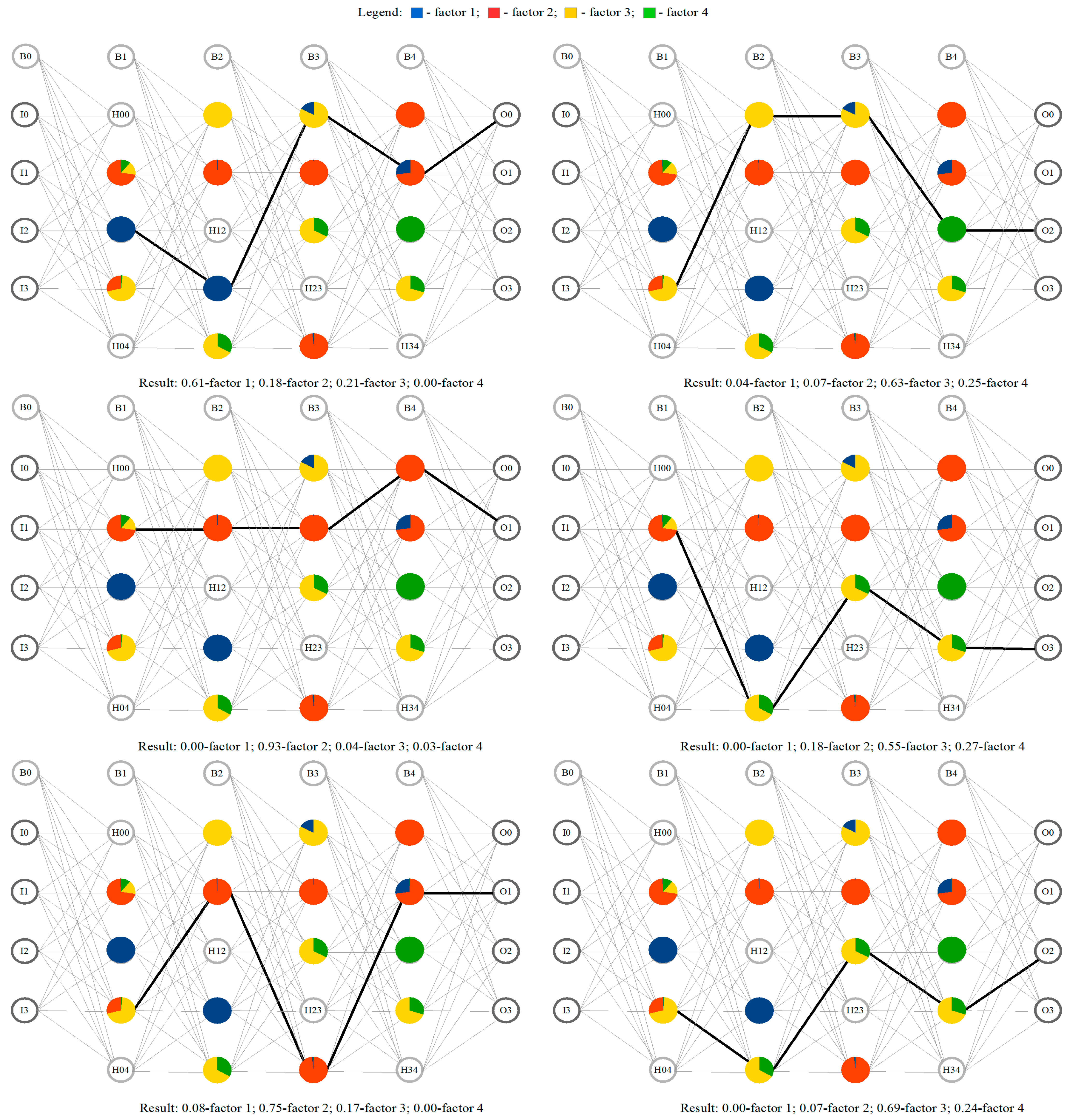
Then, in the next stage (8), we can finally form the corresponding reverse chains of the maximal weights, starting from the correct active output layer’s neuron, continuing back through all the hidden layers, and finalizing by the corresponding input layer’s neuron. For this purpose, in the scope of the current research, the corresponding additional dedicated software was developed in Python as well. An output results example, obtained by this developed Python software, is presented below in Figure 5.

As the operation result of this dedicated developed Python software, the following results were obtained, as presented in

Table 2. Obtained reverse chains of neurons for related impact factor(s).

Obtained Reverse Chains of Neurons for Related Impact Factor	Related Impact Factor
O[0] < -HLN[3][1] < -HLN[2][0] < -HLN[1][3] < -HLN[0][2] < -I[2] O[0] < -HLN[3][1] < -HLN[2][0] < -HLN[1][3] < -HLN[0][2] < -I[3] O[0] < -HLN[3][1] < -HLN[2][0] < -HLN[1][3] < -HLN[0][2] < -I[1] O[0] < -HLN[3][1] < -HLN[2][0] < -HLN[1][3] < -HLN[0][2] < -I[0] O[0] < -HLN[3][1] < -HLN[2][1] < -HLN[1][1] < -HLN[0][3] < -I[1] O[0] < -HLN[3][1] < -HLN[2][4] < -HLN[1][1] < -HLN[0][1] < -I[2]	Impact factor 1
O[1] < -HLN[3][0] < -HLN[2][1] < -HLN[1][1] < -HLN[0][1] < -I[3] O[1] < -HLN[3][1] < -HLN[2][4] < -HLN[1][1] < -HLN[0][3] < -I[1] O[1] < -HLN[3][0] < -HLN[2][1] < -HLN[1][1] < -HLN[0][1] < -I[2] O[1] < -HLN[3][1] < -HLN[2][4] < -HLN[1][1] < -HLN[0][1] < -I[2] O[1] < -HLN[3][0] < -HLN[2][1] < -HLN[1][1] < -HLN[0][3] < -I[1] O[1] < -HLN[3][0] < -HLN[2][1] < -HLN[1][1] < -HLN[0][3] < -I[0] O[1] < -HLN[3][1] < -HLN[2][4] < -HLN[1][1] < -HLN[0][3] < -I[0]	Impact factor 2
O[2] < -HLN[3][3] < -HLN[2][0] < -HLN[1][0] < -HLN[0][3] < -I[1] O[2] < -HLN[3][3] < -HLN[2][2] < -HLN[1][4] < -HLN[0][3] < -I[1] O[2] < -HLN[3][2] < -HLN[2][0] < -HLN[1][0] < -HLN[0][3] < -I[1] O[2] < -HLN[3][3] < -HLN[2][2] < -HLN[1][4] < -HLN[0][1] < -I[2] O[2] < -HLN[3][2] < -HLN[2][0] < -HLN[1][0] < -HLN[0][3] < -I[0] O[2] < -HLN[3][3] < -HLN[2][0] < -HLN[1][0] < -HLN[0][3] < -I[0] O[2] < -HLN[3][2] < -HLN[2][2] < -HLN[1][4] < -HLN[0][1] < -I[2] O[2] < -HLN[3][2] < -HLN[2][2] < -HLN[1][4] < -HLN[0][1] < -I[3] O[2] < -HLN[3][2] < -HLN[2][2] < -HLN[1][4] < -HLN[0][3] < -I[1]	Impact factor 3
O[3] < -HLN[3][3] < -HLN[2][2] < -HLN[1][4] < -HLN[0][1] < -I[2] O[3] < -HLN[3][3] < -HLN[2][2] < -HLN[1][4] < -HLN[0][3] < -I[1] O[3] < -HLN[3][1] < -HLN[2][4] < -HLN[1][4] < -HLN[0][1] < -I[2]	Impact factor 4

below.

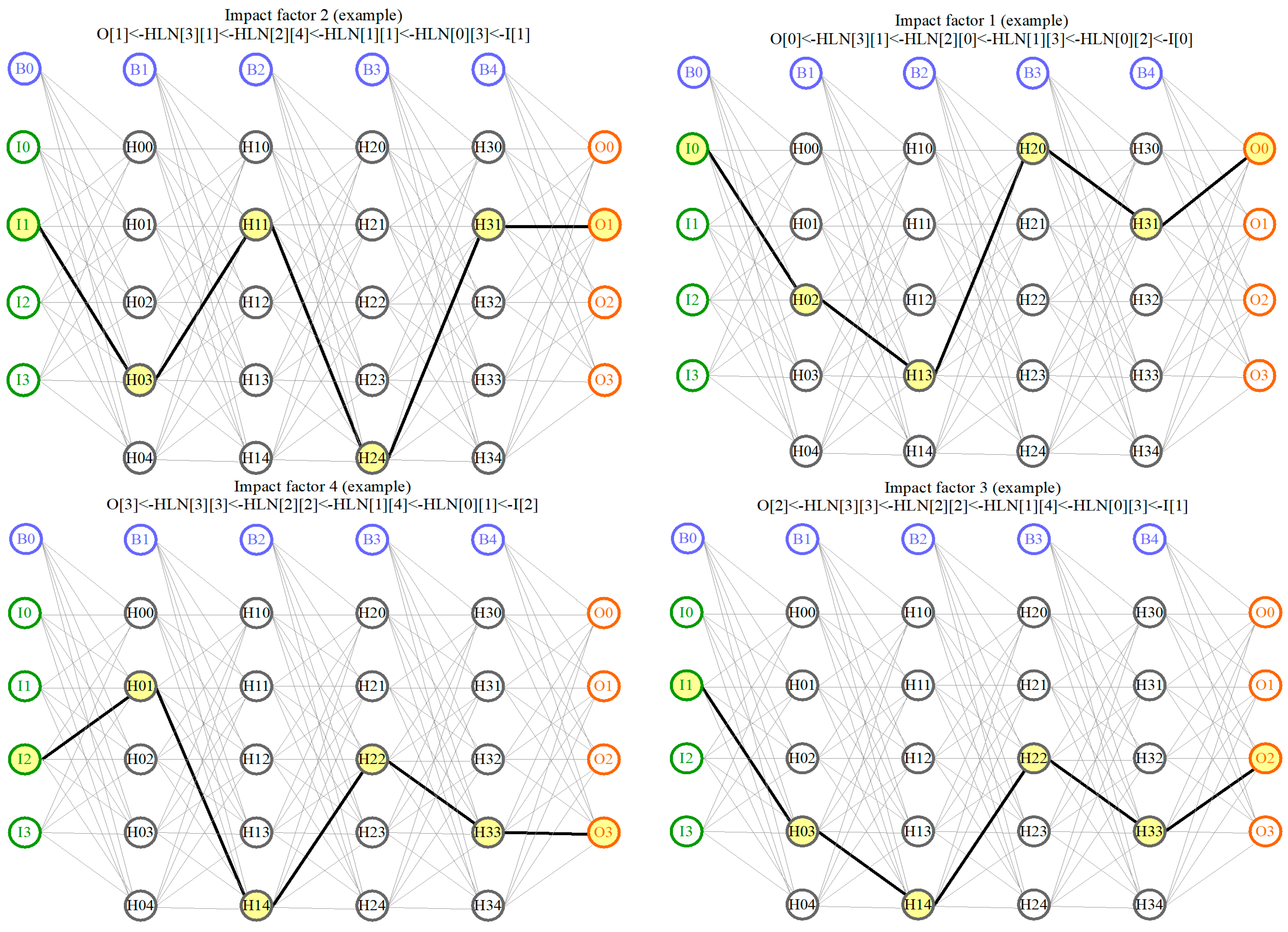
For better clarity and understanding of the obtained resulting reverse chains, Figure 6 below shows graphic visualizations of a few of them as an example.

Since the input layer’s neurons I0–I3, as well as the output layer’s neurons O0-O3, are actually of no interest from the point of view of their belonging to the impact factors (according to the strategy of developed method), only the belonging of the hidden layers’ neurons (to these impact factors) is of interest. Taking this into consideration, the following unique reverse chains will be obtained (without input and output layers’ neurons):

• Obtained reverse chains of neurons for impact factor 1:

HLN[3][1] < -HLN[2][0] < -HLN[1][3] < -HLN[0][2]

HLN[3][1] < -HLN[2][1] < -HLN[1][1] < -HLN[0][3]

HLN[3][1] < -HLN[2][4] < -HLN[1][1] < -HLN[0][1]

• Obtained reverse chains of neurons for impact factor 2:

HLN[3][0] < -HLN[2][1] < -HLN[1][1] < -HLN[0][1]

HLN[3][1] < -HLN[2][4] < -HLN[1][1] < -HLN[0][3]

HLN[3][1] < -HLN[2][4] < -HLN[1][1] < -HLN[0][1]

HLN[3][0] < -HLN[2][1] < -HLN[1][1] < -HLN[0][3]

• Obtained reverse chains of neurons for impact factor 3:

HLN[3][3] < -HLN[2][0] < -HLN[1][0] < -HLN[0][3]

HLN[3][3] < -HLN[2][2] < -HLN[1][4] < -HLN[0][3]

HLN[3][2] < -HLN[2][0] < -HLN[1][0] < -HLN[0][3]

HLN[3][3] < -HLN[2][2] < -HLN[1][4] < -HLN[0][1]

HLN[3][2] < -HLN[2][2] < -HLN[1][4] < -HLN[0][1]

HLN[3][2] < -HLN[2][2] < -HLN[1][4] < -HLN[0][3]

• Obtained reverse chains of neurons for impact factor 4:

HLN[3][3] < -HLN[2][2] < -HLN[1][4] < -HLN[0][1]

HLN[3][3] < -HLN[2][2] < -HLN[1][4] < -HLN[0][3]

HLN[3][1] < -HLN[2][4] < -HLN[1][4] < -HLN[0][1]

Thus, as shown in Figure 6 above (with a graphical visualization of reverse chain examples), we can label the neurons included in these chains with markers of the corresponding impact factors based on each of the obtained reverse chains. This actually completes stage 9 of the developed impact factor analysis method.

4.3. Calculating the Probabilities of the Disputed Neurons Belonging to the Competing Impact Factors

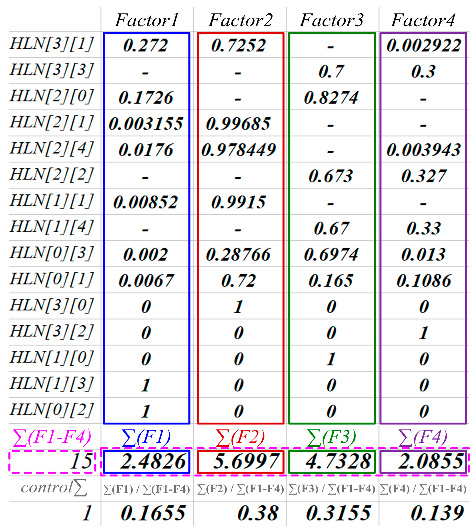
So, at this moment, it only remains to perform the final stage 10 with the calculation of the probabilities (for all neurons, obtained in previous stage) of their belonging to those impact factors to which they were appropriately labeled in the previous stage.

As can be seen from the above-presented list of unique reverse chains, a significant number of neurons were labeled with various multiple impact factors. For example:

• Neuron HLN[3][1] simultaneously belongs to impact factors 1, 2 і 4;
• Neuron HLN[3][3] simultaneously belongs to impact factors 3 і 4;
• Neuron HLN[2][0] simultaneously belongs to impact factors 1 і 3;
• Neuron HLN[2][1] simultaneously belongs to impact factors 1 і 2;
• Neuron HLN[2][4] simultaneously belongs to impact factors 1, 2 і 4;
• Neuron HLN[2][2] simultaneously belongs to impact factors 3 і 4;
• Neuron HLN[1][1] simultaneously belongs to impact factors 1 і 2;
• Neuron HLN[1][4] simultaneously belongs to impact factors 3 і 4;
• Neuron HLN[0][3] simultaneously belongs to impact factors 1, 2, 3 і 4;
• Neuron HLN[0][1] simultaneously belongs to impact factors 1, 2, 3 і 4.

This means that there is some number of disputed neurons, for which it is necessary to calculate the probability of their belonging to each of the competitive impact factors.

The main recommendation for minimizing the number of disputed neurons and competitive impact factors is to increase the dimensionality of the hidden layers’ neuron matrix and the constant experimental research in this direction (in a similar way to that conducted during the design of any multilayer perceptron models, where the number of hidden layers, as well as the number of neurons on these hidden layers, is often chosen mainly experimentally). However, in this research, we deliberately consider the case with a significant number of disputed neurons (as in our presented experimental case: 50% of all the hidden layer neurons of the MP model are actually disputed, and this is really quite a high rate) in order to better illustrate the process of calculating the probabilities of the belonging of these disputed neurons to appropriate competitive impact factors.

So, for our considered specific experimental case, we obtained the following values, calculated according to the above-mentioned expressions: FI[1] = 0.06476, FI[2] = 0.471928, FI[3] = 0.40652, and FI[4] = 0.056792; such exact values were obtained as an operation result of the appropriate additional specially developed Python software for calculating the influence indexes of each of the four impact factors of the developed model, as presented in this research, obtained on a million-dataset (a dataset of 1 million records).

Table 3. Results of calculations for obtained reverse chains of impact factors.

FoA_Global	FI	FoA_Local	Impact Factor #
			Impact factor 1
0.0607	0.06476	0.93737	HLN[3][1] < -HLN[2][0] < -HLN[1][3] < -HLN[0][2]
0.0009464	0.06476	0.014614	HLN[3][1] < -HLN[2][1] < -HLN[1][1] < -HLN[0][3]
0.00310848	0.06476	0.048	HLN[3][1] < -HLN[2][4] < -HLN[1][1] < -HLN[0][1]
			Impact factor 2
0.233935	0.471928	0.4957	HLN[3][0] < -HLN[2][1] < -HLN[1][1] < -HLN[0][1]
0.0707892	0.471928	0.15	HLN[3][1] < -HLN[2][4] < -HLN[1][1] < -HLN[0][3]
0.10194	0.471928	0.216	HLN[3][1] < -HLN[2][4] < -HLN[1][1] < -HLN[0][1]
0.065126	0.471928	0.138	HLN[3][0] < -HLN[2][1] < -HLN[1][1] < -HLN[0][3]
			Impact factor 3
0.026	0.40652	0.064	HLN[3][3] < -HLN[2][0] < -HLN[1][0] < -HLN[0][3]
0.037277884	0.40652	0.0917	HLN[3][3] < -HLN[2][2] < -HLN[1][4] < -HLN[0][3]
0.26505	0.40652	0.652	HLN[3][2] < -HLN[2][0] < -HLN[1][0] < -HLN[0][3]
0.06864	0.40652	0.16885	HLN[3][3] < -HLN[2][2] < -HLN[1][4] < -HLN[0][1]
0.00828488	0.40652	0.02038	HLN[3][2] < -HLN[2][2] < -HLN[1][4] < -HLN[0][1]
0.0011789	0.40652	0.0029	HLN[3][2] < -HLN[2][2] < -HLN[1][4] < -HLN[0][3]
			Impact factor 4
0.04997696	0.056792	0.88	HLN[3][3] < -HLN[2][2] < -HLN[1][4] < -HLN[0][1]
0.00612445	0.056792	0.10784	HLN[3][3] < -HLN[2][2] < -HLN[1][4] < -HLN[0][3]
0.00069598596	0.056792	0.012255	HLN[3][1] < -HLN[2][4] < -HLN[1][4] < -HLN[0][1]

below shows the results of the calculations executed for each reverse chain of each of the impact factors of the presented developed example experimental model considered in this research.

Returning back to our example, the following specific numerical probability values of the belonging of each of the disputed neurons to their respective competing impact factors were obtained; they are given in

Table 4. The probability result calculations of the belonging of the neurons to the impact factors.

Probability (min = 0; max = 1) of Belonging to the Impact Factor
4	3	2	1	Disputed neuron
0.0029221	-	0.7252	0.272	HLN[3][1]
0.3	0.7	-	-	HLN[3][3]
-	0.8274	-	0.1726	HLN[2][0]
-	-	0.99685	0.003155	HLN[2][1]
0.0039425	-	0.978449	0.0176	HLN[2][4]
0.327	0.673	-	-	HLN[2][2]
-	-	0.9915	0.00852	HLN[1][1]
0.33	0.67	-	-	HLN[1][4]
0.013	0.6974	0.28766	0.002	HLN[0][3]
0.1086	0.165	0.72	0.0067	HLN[0][1]
4	3	2	1	Not-disputed neuron
0	0	1	0	HLN[3][0]
1	0	0	0	HLN[3][2]
0	1	0	0	HLN[1][0]
0	0	0	1	HLN[1][3]
0	0	0	1	HLN[0][2]

below.

Figure 7 below provides a graphical representation of the obtained probability calculation results of the belonging of the hidden layer neurons to the relevant impact factors of the developed model considered in this research as an example.

Now, having the probabilities of the belonging of the corresponding MP model neurons to the impact factors of the relevant supported object’s subjective perception model, we can determine the impact level for each impact factor’s influence on the perception results of the investigated support object (supported software complex or the processes of its support) by the relevant subject(s) of interaction (with it), for each individual modeling case. In Figure 8 below, there are also presented visualized examples of the calculated impact factors’ fraction(s) as appropriate results of the researched object’s perception by the corresponding subject of interaction with it.

Thus, in this way, by means of the developed impact factors reverse analysis method, we managed to form (restore or recreate) certain boundaries of the influence of various impact factors which affect the subjective perception results of the supported software complex or the processes of its comprehensive support, caused by the distortion of its input objective characteristics and their further transformation into the resulting output subjective characteristics of its subjectivized representation.

Also, as was already mentioned earlier in this research, according to the developed method we consider all the input data for modeling in depersonalized (without any functional–semantic meanings) and normalized forms of representation, as, first of all, from a scientific and research point of view, we are mainly interested in the very process of the impact factor analysis itself, in its possibilities and potential. Accordingly, the purpose of the data does not have such an important meaning for us in this case. Moreover, in the absolute majority of cases in real conditions (in real companies and when solving real practical applied problems) all the data usually come for processing in a maximally depersonalized form, caused, first of all, by relevant primarily practical approach (as in most cases, they can represent sensitive personal information or customers’ commercial secrets). Of course, the original data for training and testing usually undergo some primary processing, performed either on the client’s/customer’s side or on the developer’s side, but this is conducted only by a limited circle/group of employees provided with special contracted access (to these original data). Later, however, all these original data should mandatorily undergo thorough and complete depersonalization, and only on this basis should the appropriate model’s input data be formed. Regarding data normalization, this stage can be carried out on either the client’s/customer’s side or on the developer’s side without any permission restrictions as it is devoid of any sensitivity of incoming information since at this moment it already comes in a depersonalized form.

In this way, the boundaries of the impact factors are restored for each individual investigated subject of interaction with the supported software complex. As a result, at the output of the developed method we receive specific numerical values for each investigated subject (which interacts with the supported software complex), and these obtained values actually provide us with a clear specific characteristic for each of these subjects. Later, depending on the applied field(s) of the type of developed method usage, obtained numeric values are used to solve a relevant specific practical applied problem. Examples of such applied areas of the developed method usage include (but are not limited to) such tasks as the following:

• Determination of parametric indicators of subjects interacting with the supported software complex (a kind of specific individual “portrait” of each subject);
• Development of virtual models of the subjects (interacting with the supported software complex and providing its support) based on their parametric indicators;
• Development of virtual assistant(s) with a set of given indicators (with which cooperating with such an assistant would be as comfortable as possible for the subjects);
• Determination of advantages and disadvantages (that is, weaknesses and strengths) of each support team member (which is, at the same time, a subject of interaction with the supported software complex) in order to identify areas, fields, and/or directions of potential self-improvement(s) for considered support team members;
• Simulation (and prediction) of potential conflict situations based on identified weaknesses of researched support team members;
• Selection of the specific support team member(s) most suitable for a specific supported software complex(es);
• Selection of the specific support team member(s) most suitable for the specific client(s)/customer(s) or specific task(s);
• Support team members’ categorization according to their parametric indicators;
• Formation of support team(s) based on their parametric indicators and/or parametric indicators of their members;
• Determination of complementary and interchangeable members of support team(s);
• Determination of client(s)/customer(s) employees’ (who are the end users of the supported software complex) portraits;
• Development the relevant model(s) of clients and/or clients’ users that would allow the provision of further possibilities for automated internal audit of provided support quality for the supported software complex(s);
• And many others.

4.4. Example of a Practical Task Resolution by the Developed Method

In particular, in the scope of this research, as an example, the practical task of the support team members’ portrait determination is solved, followed by a further search (detection) of the interchangeable members of this team to ensure the possibility of a quick transfer of a stack of tickets (which are in the middle of the active resolution process) between these members. The main problem during this kind of ticket transferring consists in a colossal loss of the processes’ efficiency coefficient, especially during such an unplanned (forced) transfer of tickets between team members. This is mainly caused by the fact that quite often each new recipient of the ticket(s) must actually start solving it from the very beginning, e.g., from scratch (as it is extremely complicated to quickly and carefully figure out and understand what has already been done by the previous “ticket-holder” employee, and what his/her further plans were regarding this ticket). That is why it is so important to choose a new receiver whose point of view on the issue of the considered ticket(s) (and, ideally, view on the whole supported software complex as well) is close (as possible) to the point of view of the previous “ticket-holder”.

So, in order to resolve the given practical task, the developed method was applied for all the support team members in order to form their appropriate individual portraits (based on the obtained parametric indicators), which (portraits) are actually the results matrix (for each member) with the calculated probabilities of the hidden layer neurons belonging to the declared impact factors of the developed model. These data are certainly important for further in-depth analysis. However, in our case, they are only intermediate data for obtaining the final result: quantitative characteristics (in percentage) for each of the impact factors. That is, in other words, the summation of the obtained probability values of the belonging of each of the neurons to each of the impact factors is performed. This process can be visualized using the example of Table 4 above, where the values in the columns (representing each of the impact factors) should just be summed up. In this way, the total probability values for the belonging of the neurons to each of the identified impact factors (in our considered research case, the number of such factors = 4—see Table 4) will be obtained. After that, all these total values are converted from absolute to relative in order to provide the possibility of their further comparison with the same values for all the other investigated subjects of interaction with the same supported software complex. Figure 9 below shows an illustrative interpretation of the described process of calculating the researched subject’s comparative portrait.

Following the same scenario, the formation of the comparative portraits of all the other investigated subjects (interacting with the researched supported software complex) is performed as well.

Table 5. Obtained comparative portrait calculation data for all investigated subjects.

Factor 4	Factor 3	Factor 2	Factor 1
0.139	0.3155	0.38	0.1655	Subject 1
0.1062	0.562	0.2069	0.1249	Subject 2
0.1224	0.2277	0.4954	0.1545	Subject 3
0.1354	0.4261	0.1752	0.2633	Subject 4
0.1682	0.2976	0.1981	0.3361	Subject 5
0.2174	0.3256	0.2649	0.1921	Subject 6
0.2311	0.2972	0.2891	0.1826	Subject 7
0.2059	0.4188	0.2684	0.1069	Subject 8
0.2549	0.1672	0.3582	0.2197	Subject 9
0.2739	0.1978	0.403	0.1253	Subject 10
0.1964	0.1774	0.2095	0.4167	Subject 11
0.3529	0.1415	0.3718	0.1338	Subject 12
0.2294	0.3152	0.3641	0.0913	Subject 13
0.0912	0.367	0.4912	0.0506	Subject 14
0.2145	0.1892	0.2912	0.3051	Subject 15

below represents the data obtained from the calculations of the comparative portraits for all investigated subjects.

Also, in Figure 10 below, the obtained calculation data (for all investigated subjects) for the comparative portraits are presented in the form of a corresponding general histogram for better visual perception.

Table 6. Table of interchangeable subjects’ definition.

S15	S14	S13	S12	S11	S10	S9	S8	S7	S6	S5	S4	S3	S2	S1
0.43	0.325	0.18	0.428	0.617	0.316	0.34	0.34	0.218	0.23	0.4	0.417	0.231	0.493	-	S1
0.746	0.569	0.561	0.841	0.769	0.728	0.79	0.32	0.53	0.473	0.546	0.335	0.669	-	0.493	S2
0.485	0.279	0.389	0.461	0.672	0.303	0.395	0.549	0.413	0.461	0.595	0.64	-	0.669	0.23	S3
0.474	0.632	0.566	0.828	0.497	0.733	0.605	0.327	0.419	0.343	0.26	-	0.64	0.335	0.417	S4
0.279	0.725	0.49	0.717	0.24	0.621	0.494	0.458	0.308	0.288	-	0.257	0.595	0.546	0.4	S5
0.279	0.535	0.222	0.485	0.449	0.389	0.317	0.193	0.08	-	0.288	0.343	0.461	0.473	0.23	S6
0.249	0.544	0.186	0.409	0.468	0.313	0.26	0.243	-	0.08	0.308	0.419	0.413	0.53	0.218	S7
0.459	0.446	0.238	0.555	0.62	0.442	0.503	-	0.243	0.19	0.458	0.327	0.549	0.322	0.34	S8
0.215	0.666	0.308	0.223	0.414	0.19	-	0.503	0.26	0.317	0.494	0.605	0.395	0.79	0.34	S9
0.36	0.515	0.235	0.18	0.583	-	0.189	0.442	0.313	0.389	0.621	0.733	0.303	0.728	0.316	S10
0.22	0.943	0.651	0.638	-	0.583	0.414	0.62	0.468	0.449	0.24	0.497	0.672	0.769	0.617	S11
0.438	0.69	0.347	-	0.638	0.18	0.223	0.555	0.409	0.485	0.717	0.828	0.461	0.841	0.428	S12
0.428	0.358	-	0.347	0.651	0.235	0.308	0.238	0.186	0.222	0.49	0.566	0.389	0.561	0.18	S13
0.756	-	0.358	0.69	0.943	0.515	0.665	0.446	0.544	0.535	0.725	0.632	0.28	0.569	0.325	S14
-	0.756	0.428	0.438	0.223	0.36	0.21	0.459	0.249	0.279	0.279	0.474	0.485	0.746	0.43	S15

below also presents the final results of the obtained subjects’ comparative portraits, as well as the found (detected) most optimal interchangeable subjects.

According to the obtained calculation results, the most optimal interchangeable subjects are as follows: for subject S1—subject S13; for subject S2—subject S8; for subject S3—subject S1; and so on, according to Table 6 above.

It should also be noted that solving the given task automatically solves a number of other additional tasks, such as

• Finding the most optimal pair of team members whose portraits differ minimally compared to others (in the considered case presented above, it is the pair of subjects S7–S6 with the minimum comparison value 0.08 in Table 6);
• Finding the least optimal pair of team members whose portraits have the maximum difference compared to others (in the considered case presented above, it is the pair of subjects S2–S8 with the maximum comparison value 0.32 in Table 6);
• Finding the most optimal candidate for replacement of a team member who is already replacing another previous team member;
• Finding a team member with the minimum value of the total portraits’ comparison difference with the rest of the team members (in the considered case presented above, it is subject S7) as the most universal potential “acceptor” of the considered team’s tasks’ stack;
• Finding a team member with the maximal value of the total portraits’ comparison difference with the rest of the team members (in the considered case presented above, it is subject S2) as the least universal potential “acceptor” of the considered team’s tasks’ stack;
• Providing possibilities for various division(s) of the researched team(s) into appropriate groups and/or subgroups in accordance with obtained portraits of their members;
• Determination of a generalized comprehensive portrait of whole researched team based on the individual portraits of its members, with the possibility of further correction(s);
• Determination of the deviation of team members’ portraits from the generalized comprehensive portrait of this whole team (e.g., the whole team’s portrait);
• And many others.

Thus, the specific practical task of the determination of the most optimal support team members’ replacements (to ensure the possibility of quick transfer of the stack of tasks, which are in the middle of the active resolution phase, between the most interchangeable team members) is solved with the help (and by means) of the developed and presented method.

So, as can be seen from the performed research, the potential of the developed impact factors reverse analysis method (for software complexes’ support automation and intellectualization) is extremely significant both in solving the scientific and applied problem of software complexes’ support automation and for solving a huge number of relevant related applied practical tasks. Among such applied tasks, there is also the one solved and provided in this research as a demonstrative example—a practical task of the support team members’ portrait determination, followed by a further search (detection) of the interchangeable members of this support team to ensure the possibility of quick transfer of the stack of tickets (which are in the middle of the active resolution process) between these members.

4.5. Comparison with Outcome of Existing Similar Approaches

Additionally, comparing the developed and proposed approach with an existing one [51] (where the relevant approach was represented, dedicated for measuring perceptions of various impact factors that affect software development team performance) confirms a number of advantages, including the following:

• The presence of built-in artificial intelligence which is based on multilayer perceptron neural networks;
• The provision of hidden layer neurons (of encapsulated models of a multilayer perceptron) with functional and semantic load/meaning in the context of researched impact factors;
• The availability of research opportunities not only for studying subjective perception of impact factors affecting a supported object (e.g., developed software), but also for studying subjective perception (caused by these impact factors) of the supported object itself.

In the future, additional studies and research will be conducted, related to the application of the developed method for solving other scientific and applied practical problems and tasks in the direction of software complexes’ comprehensive support automation and intellectualization.

In addition, one of the potential directions of further investigation is researching potential ways of improvement(s) based on calculating the number of hidden layer neurons (e.g., calculating some “optimal hidden layers’ configuration” of an encapsulated multilayer perceptron model in the scope of the developed method) in order to improve the results obtained by the developed method, because at this moment, in general, the quality of the obtained results depends on the number/amount of “disputed neurons” and “competing impact factors”. So, the “ideal conditions” for the method involve reducing the total amount of such cases to zero (so that one separate hidden layer neuron would belong to only one exact separate impact factor). But in situation(s) where there is a large (like, for example, ≥10) number of “competing impact factors” for only one specific separate “disputed neuron”, it might occur that some “belonging probability value(s)” would appear so “small” (like, for example, ≤0.001) that they could be treated as a “classical statistical error”, but later they could affect the quality of the results obtained by the method. So, theoretically, when the number of neurons in hidden layers is greater, it could increase our chances that less impact factors will “compete” for a single neuron. But the “tricky” thing here is that we never know how many “disputed neurons” and “competing impact factors” we will obtain before finalizing and processing the existing related datasets and analyzing all the obtained reverse chains. So, the situation described here is similar to the “classic dilemma” with a multilayer perceptron: the researcher (e.g., neural network designer) never knows (in advance) exactly how many hidden layer neurons will be needed until a full cycle of training and testing is finalized, and only after that (based on acquired practical heuristic experience) can the researcher finally find the best configuration. That is why calculating an optimal hidden layer configuration of an encapsulated multilayer perceptron model in the scope of the developed method is one of an actual scientific direction for further investigations in the scope of the declared researched area, as presented in this paper.

5. Conclusions

The developed impact factors reverse analysis method for software complexes’ support automation is presented in this research. It provides possibilities for analysis of the influence performed on the supported software complexes (as well as on the processes of their comprehensive support) by the relevant pre-determined impact factors. Also, the developed method allows the restoration of the influence boundaries of the impact factors in the corresponding models of software complexes’ support, which is developed and presented in this research as well. In addition, the developed method is suitable for solving a batch of applied practical problems (tasks) described in this research. An appropriate primary generalized model of the supported object’s subjective perception and the algorithm for the impact factors reverse analysis method, as well as the mathematical component of the impact factors reverse analysis method, have been developed and presented in this research as well. Each of the stages of the developed algorithm is considered in detail in the scope of this research, as well as all the questions, specifics, and aspects related to the format, structure, and processing of the data needed for the developed method’s correct and effective functional operation.

According to the developed method, the analysis of impact factors is performed on the basis of multilayer perceptron artificial neural network(s), as well as the constructed reverse chains with maximal weights between

• Output subjective characteristics of the perception’s results of the supported object or process (represented by neurons of MP’s output layer);
• All intermediate layers of input characteristics’ transformation into the relevant output characteristics (but mandatory in reverse order: from the final such layer, back to the initial one) represented by neurons of MP’s hidden layers;
• Corresponding input characteristics of the researched supported object or process (e.g., software complex or processes of its comprehensive support) represented by the neurons of MP’s input layer.

Subsequently, by means of the developed method, appropriate quantitative and structural classification of the multilayer perceptron(s) hidden layer neurons was obtained based on relation(s) with their belonging to the corresponding pre-determined impact factors. In turn, this provides possibilities for carrying out an automated analysis and quantitative assessment of the level of influence, performed by various impact factors, on the results of the supported object’s (the supported software complex, as well as the processes of its comprehensive support) perception by appropriate subjects, which directly or indirectly interact with it.

Thus, the results obtained by resolving the task of impact factor analyses, presented in the scope of this research, are extremely important for further research and solving a much more complex and difficult scientific and applied problem of software complexes’ support automation. In addition, the practical task of the support team members’ portrait determination, followed by a further search (detection) of the interchangeable members of this support team to ensure the possibility of quick transfer of the stack of tickets (which are in the middle of the active resolution process) between these members, was solved and represented in this research as a practical application example of the developed method.

Therefore, the developed method also solves the problem of restoring the boundaries of the impact factors inside the relevant models of software complexes’ support, after these boundaries have been blurred or lost as a result of the introduction and the application of a multilayer perceptron (for ensuring additional self-learning functionality for these models) into these models. Among other things, this significantly contributes to the resolution of the software complexes’ support automation problem.

Therefore, in the future, the authors plan to continue the studies and research in the same direction of the software complexes’ support automation by further application and improvements of the developed method. In addition, the developed method appeared to be extraordinarily universal; so, it can be additionally used not only in the field(s) of software products’ support (and information technologies in general), but also in quite different fields, such as, in particular, psychology, sociology and others, as well as the relevant related interdisciplinary areas like IT + psychology, IT + sociology, IT + human resources, IT management, human–machine interface, human-centered design, human factors evaluation, etc. This can be seen by the obtained method approbation’s results in the scope of the resolved applied practical task considered and presented in the scope of this research.

One of potential common solutions for the problem of the aforementioned areas is the adaptation of the developed method to each of these areas by researching, substantiating, selecting, and declaring the appropriate sets of impact factors, since the developed method is quite universal and flexible (which is its additional benefit/advantage); so, depending on the selected set of impact factors, it provides possibilities for researching the influence of these factors (on the researched object) without any strict limitations on the selected area of the research itself.