Flexibly Parameterizable Vehicle Dynamics Models

Abstract

The following article presents the longitudinal modeling and simulation of a generic electric vehicle. The purpose of the research is to describe the applied modeling procedures and their MATLAB solutions. Furthermore, the goal is to demonstrate how to build a framework for a MATLAB R2024b Simulink and Simscape model that facilitates future optimization and ensures modularity, thereby facilitating collaboration among different research groups. After presenting the applied vehicle dynamics model and the created framework, some additional application examples are presented for which the method has already been tested.

1. Introduction

In the ever-developing scientific fields of today, it is increasingly challenging to achieve new scientific results. Individual researchers are unable to keep up; therefore, it becomes necessary to work as part of research groups and for these research groups to collaborate with each other. The over-the-wall method, just like the methodical machine and product design, is proving to be outdated in research as well. In order to increase efficiency, it becomes necessary to find a solution so that research groups can work in parallel. For parallelization, a framework must be provided that creates an interface between research groups without having to deeply acquire the knowledge of the other research group. In our case, a research group dealing with vehicle dynamics simulations and a research group responsible for optimization used this framework.

During the literature review, we found only a few publications closely related to the present research. The MATLAB System Composer application gives system engineers the opportunity to code in parallel with respect to very complex system models. Although this application is an effective method for the parallel development of complex systems, it cannot be used for the problem presented in this research. This is because, in the case discussed in this research, instead of the parallel development of the model, the goal is its multidisciplinary use. MATLAB System Composer was successfully used by del-Olmo et al. [1] to create an educational resource for systems engineering master’s students. In Korsunovs et al.’s research [2], a process FMEA generation system was created using model-based system design (MBSE). In the research of Erpyleva and colleagues [3], they used the above-mentioned MATLAB tool to analyze the error propagation of aircraft systems. Watkins et al. [4], through their research at Gulfstream Aerospace Corporation, developed the electronic system architecture modeling (eSAM) method using the MATLAB System Composer tool.

Publications on vehicle simulation can be divided into a few main groups. The following research [5] deals with the analysis of drivetrains equipped with hybrid, electric, or internal combustion engines. Another main group is publications dealing with control [6,7,8], which can be divided into further subgroups such as braking and maneuvering control [9,10,11,12,13,14,15] and torque vectoring [16,17,18,19]. Publications dealing with batteries and their charging and cooling are also a fairly extensive part of such research [20,21,22,23,24]. In-wheel motors are one of the most interesting research topics of recent times [18,25,26,27,28,29,30].

In the research of Crolla and Cao [5], the impact of the suspension energy regeneration is discussed. Novellis et al. [8] compared the experimental test results of the electric motor-based actuation of the direct yaw moment controller with those derived from the friction brake-based actuation of the same algorithm. In the research in [10], a model-based range extender control system can be found, with the help of which the authors found the optimal slip ratio of the wheels, as well as the copper and iron losses of the motors. The results were validated with experiments. Ivanov et al. [11] produced a comprehensive literature review of the field of ABS and TSC systems in fully electric vehicles with individually controlled electric motors. Voser et al. [12] analyzed stable states during drifting. In this research, a bicycle model and a Fiala tire model were used, with said models validated in a test bed. An autonomous drift controller was designed with linearization around the balance point of the drift. In the created loop control, the steering was used to control the yaw rate, which was used to control the sideslip. Ataei et al., in their study [13], present an integrated multi-purpose controller developed for electric vehicles using a model predictive control (MPC) approach, which achieves four main control objectives simultaneously, i.e., slip control in traction and braking, lateral stability control, handling improvement, and rollover prevention. Edrén et al.’s study [14] covers several topics. The subject of the investigation is the increase in energy efficiency, which was achieved by optimizing the control of four in-wheel motors. Their findings highlight that the required torque must be distributed evenly across the four wheels in order to maximize efficiency. A similar result was reached by Gu et al. [25]. In Zhang et al.’s research [15], three different control strategies were investigated for the purposes of regeneration efficiency and brake comfort. The results of simulations and road tests show that the maximum-regeneration-efficiency strategy, which would cause issues with respect to brake comfort and brake safety, could hardly be used with the regenerative braking system adopted. De Novellis et al. developed an offline optimization procedure which assesses the performance of alternative objective functions for the optimal wheel torque distribution of a four-wheel-drive (4WD) fully electric vehicle. De Novellis et al.’s results show that objective functions based on the minimum tire slip criterion provide a better control performance than functions based on energy efficiency [17]. Filippis et al.’s study [18] demonstrated that further significant energy consumption reductions can be achieved through the appropriate tuning of the reference understeer characteristics. Behi et al.’s study [23] experimentally and numerically analyzed (COMSOL Multiphysics^® CFD) the efficiency of battery cooling methods such as natural convection, forced convection, and evaporative cooling. Zhang et al. [24] introduced the thermal management methods of lithium-ion batteries, discussing their advantages and disadvantages. In this study, the authors analyzed air, liquid, and PCM cooling and heating methods. Hori’s research [26] dealt with an electric vehicle that was made specifically for the intensive study of advanced motion control. Chen et al. [27] developed a Karush–Kuhn–Tucker (KKT)-based algorithm to find all the local optimal solutions and, consequently, the global minimum. This newly developed method was compared with the classic active-set optimization method, discussed in a different paper by the same authors [28]. Murata et al. discussed the importance of in-wheel motors in dynamic control (e.g., TCS, ABS, and ESC) [29]. Lin et al. developed a multi-objective optimal torque distribution strategy, which was tested over the NEDC drive cycle.

Compared to the ESC method, the proposed multi-objective optimal torque distribution strategy can reduce the power loss of the drivetrain while ensuring the yaw stability. In the case of the single-lane-change test, a reduction of 26.7%, and in the case of the fishhook steering test, a reduction of 13.6% were observed [30].

In industrial applications, simulations have very significant economic importance [31]. This is especially the case in the vehicle industry, since engineers cannot rely only on heuristics when developing a new vehicle type or an existing one, since without simulations, its correctness can only be verified by the production of several prototypes. In practice, we see many successful research studies on the simulation of trucks [20] or passenger vehicles [32]. Here, for example, electric drivetrains are investigated or development possibilities are explored. Moreover, several publications focus on certain elements of the electric drive. Using simulation, M. Astaneh et al. were able to reduce the temperature of battery cells by 8% and the temperature difference between modules by 16.1% compared to battery packs available on the market [21]. Some research is focused on battery cooling [22], or on the energy-efficient control itself [16] or driving style [33] while other research is aimed at examining driving comfort [6]. Pier Giuseppe Anselma investigated a general internal combustion engine vehicle and its three hybridization options on four different driving cycles. During the study, they compared the energy saving and the change in driving comfort in different simulations [7]. This is particularly important from the point of view of the end user since when buying a vehicle, we do not only make decisions based on technical parameters. There are further energy-saving opportunities in the development of power electronic systems, be it electric, hybrid, or hydrogen cell construction [34]. Measurements are essential for validating simulations. For these measurements, it is important to be able to define the environment in which the measurement is performed as best as possible. To test an ABS system, the road surface is handled in well-defined places, and the dynamic conditions of the vehicle and the wheels are measured [9]. To reduce costs and planning time, simulations are often used where a simplified model of the real system is created. Before creating the model, important output parameters have to be identified, and input variables that affect the output have to be isolated. The degree to which a variable affects the output is also important because the influence of a loss source can depend greatly on the boundary conditions. For example, this is the case with air resistance, which, depending on the speed, can range from negligible to the greatest source of loss. During this research, our goal was to create a general electric vehicle model to be optimized later. In order to apply to any optimization algorithm, the parameters are given in such a way that they can be easily modified. We will explain the approach to this in detail. The main focuses of publications are generally the model itself, its creation, and the results obtained. Our goal was to create a model that can be used well for optimization purposes, where the necessary parameters can be easily controlled. Thanks to the flexibility of the framework, it is possible to use the model in teamwork. Several tasks can be performed with it, e.g., a parameter sensitivity test, optimization, and in the development phase, an impact assessment of each parameter’s change. These constitute the novelties of the work performed.

During our research, we were confronted with the fact that there is no method proposed in the literature for connecting the work of research groups dealing with modeling and optimization. This deficiency proves the novelty of the work performed. In addition to the sensitivity test, the presented framework was used to generate the input data of an AI-based surrogate model and for optimization using a genetic algorithm (GA). The advantage of the framework is its flexibility and multi-purpose usability. By flexibility, we mean that input variables and output values can be chosen as desired from among the parameters of the model. The multi-purpose usability allows us to freely choose the structure and complexity of the model. In addition to the above applications, it is also possible to use a model with finite element analysis (FEA). In summary, the novelty of the presented method is not the vehicle dynamics model and its creation but the related framework, which promotes cooperation between research groups.

2. Materials and Methods

2.1. Drivetrain Structure

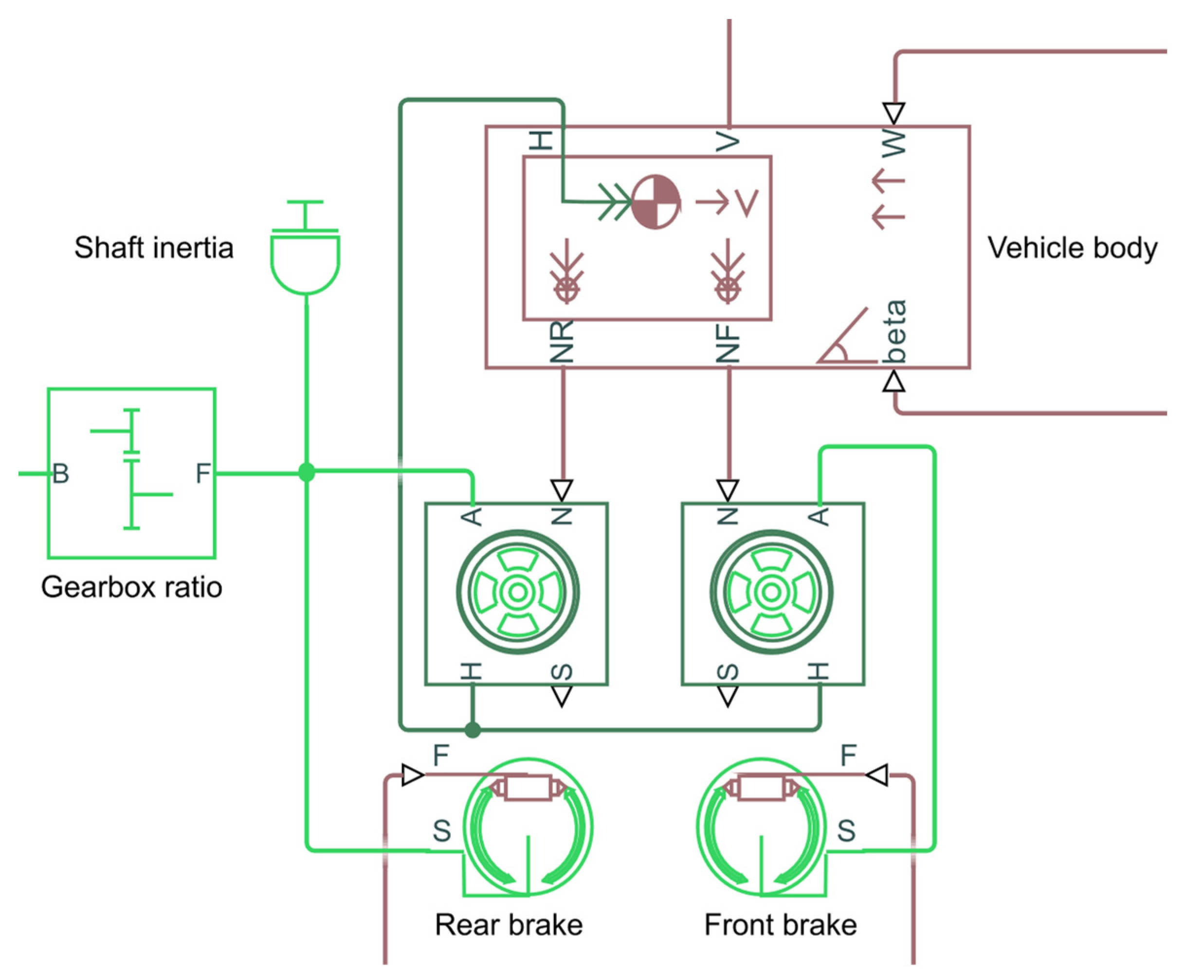
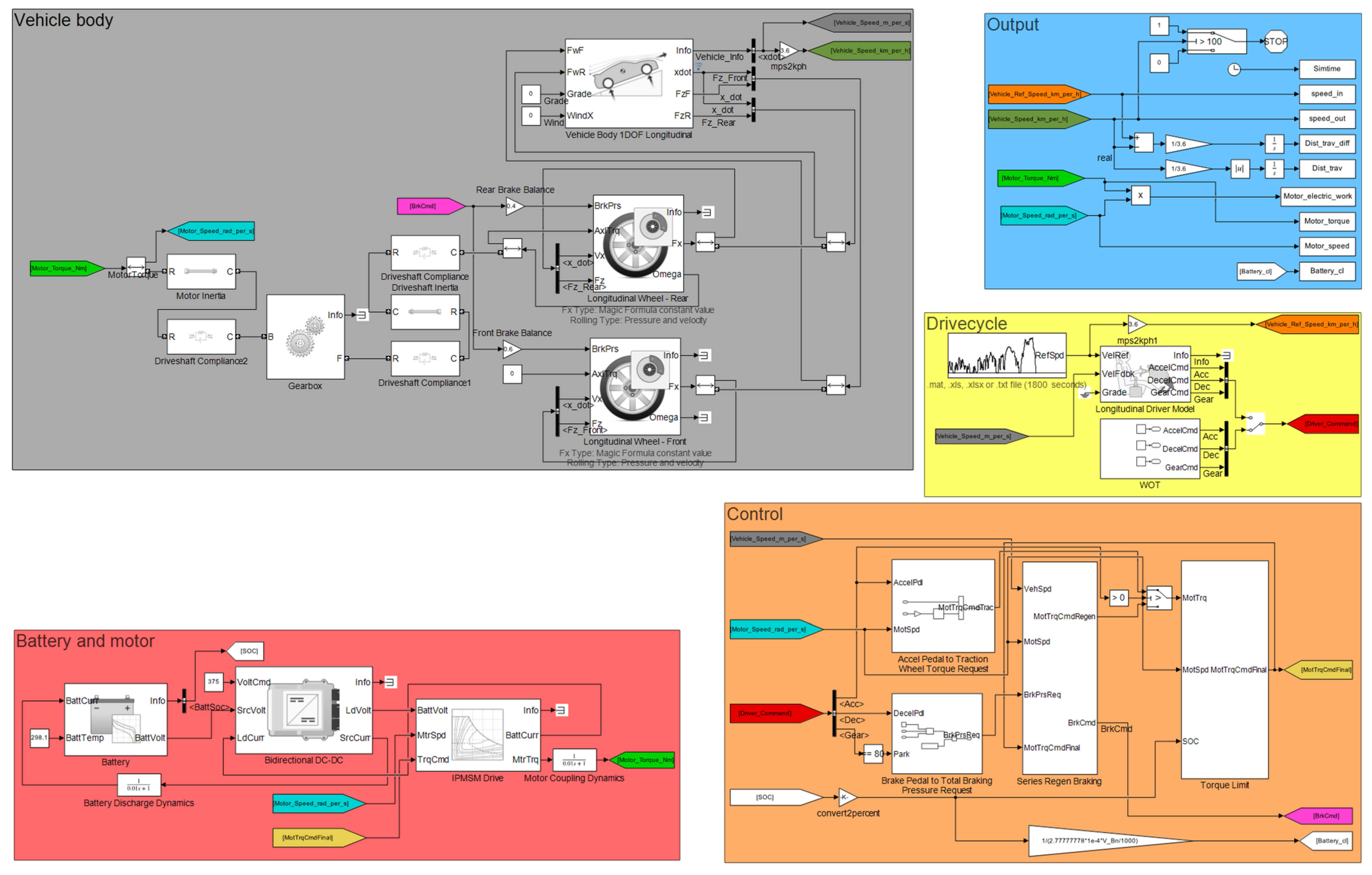
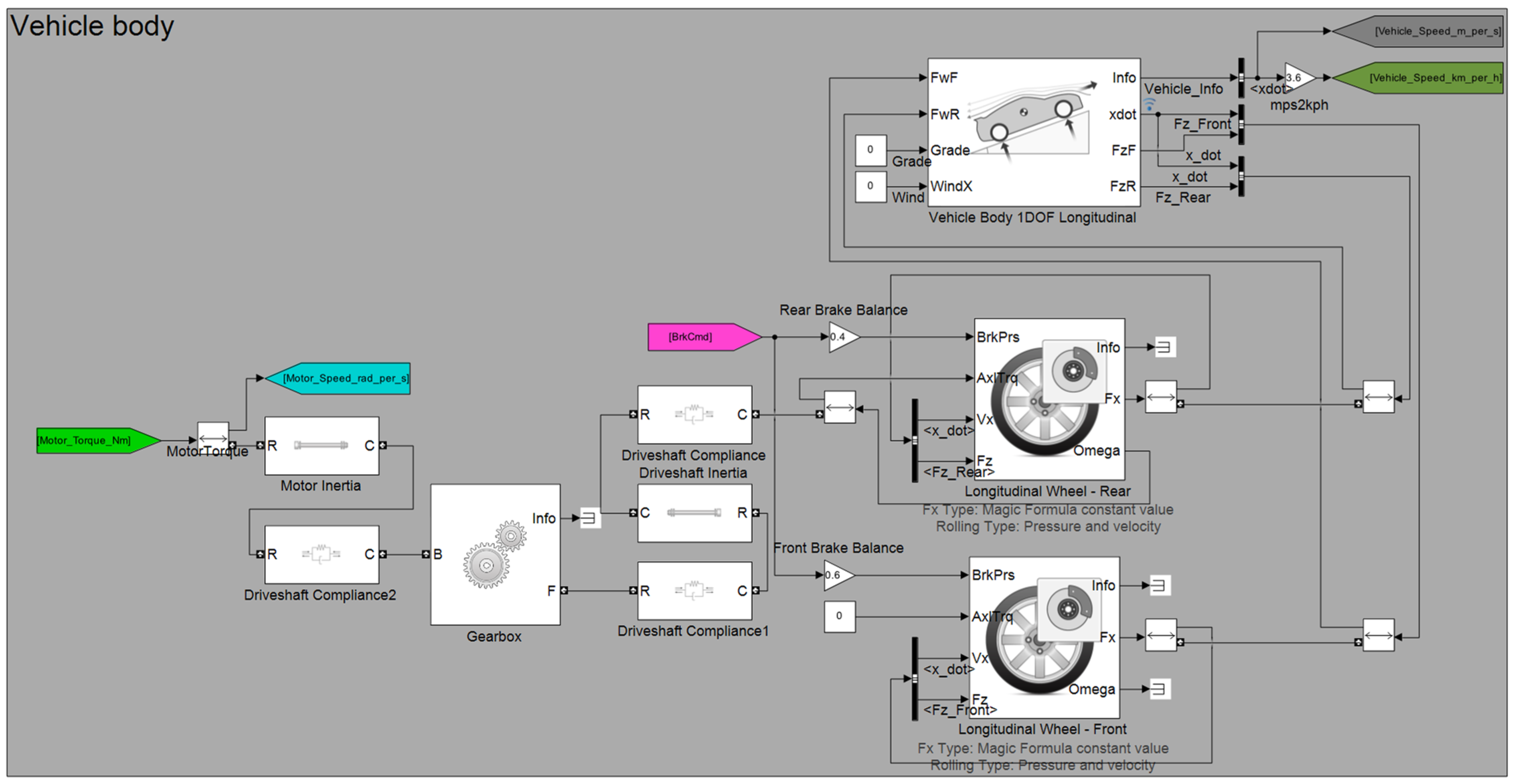
In the current phase of the research, our goal is not to validate the model. We are currently analyzing the usability of the framework, and work on validation will be relevant in the next phase of the research. The simulated electric vehicle is rear wheel driven. The vehicle body, wheels, brakes, and final drive were built using the Simulink Simscape Driveline modules. Figure 1 shows these elements of the vehicle and their connections. These modules contain the parameters required for the model and the differential equations that can be connected to them. The driving motor, energy-providing battery, and DC-DC converter were built with components from Simscape Electrical. Since this research focuses on the behavior of the drivetrain and is not justified by the length of the applied driving cycle, the battery does not contain an aging model. The torque provided by the electric motor acts on the rear wheel through the final drive. The forward movement of the front and rear wheels is connected to the vehicle body. As a result, the traction force created by the torque acting on the rear wheel acts on both the vehicle body and the wheels. The torque acting on the rear wheel is created by the driving torque, the equivalent inertia representing the inertia of the drive system, and the brake, while only the braking torque acts on the front wheel. The rolling resistances are taken into account in the tire model. A detailed description of the equations of these blocks can be found in the literature [35].

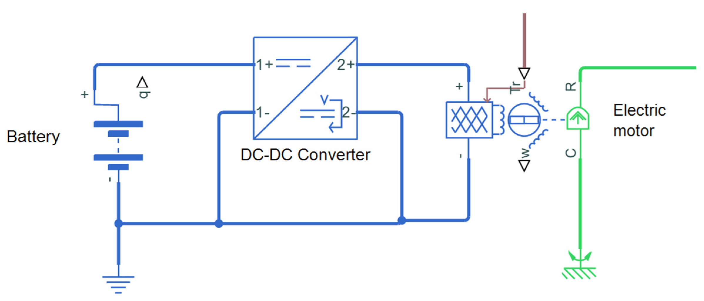
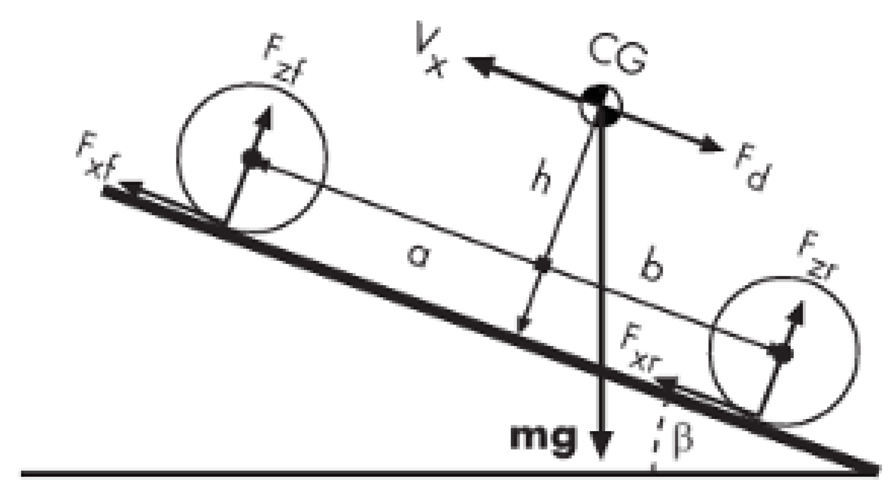
Figure 2 shows the electrical system responsible for the vehicle’s energy supply. It contains a battery and DC-DC converter. The connection between the electrical and physical domains is realized by the general engine block. Based on the MathWorks documentation, the next equations describe how the “vehicle body” block is modeled [35]. A schematic figure of the vehicle body can be seen in Figure 3. The used designations can be seen in

Table 1. Used designations [35].

Symbol	Description
$g$	Gravitational acceleration
$\beta$	Incline angle
$m$	Mass of the vehicle
$h$	Height of vehicle center of gravity (CG) above the ground
$a, b$	Distances of front and rear axles, respectively, from the normal projection point of vehicle CG onto the common axle plane
$V_x$	$\mathrm{Velocity} \mathrm{of} \mathrm{the} \mathrm{vehicle}. \mathrm{When} V_w$$> 0, \mathrm{the} \mathrm{vehicle} \mathrm{moves} \mathrm{forward}. \mathrm{When} V_x$< 0, the vehicle moves backward.
$V_w$	$\mathrm{Wind} \mathrm{speed}. \mathrm{When} V_w$$> 0, \mathrm{the} \mathrm{wind} \mathrm{is} \mathrm{a} \mathrm{headwind}. \mathrm{When} V_w$< 0, the wind is a tailwind.
$n$	Number of wheels on each axle
$F_{xf}, F_{xr}$	Longitudinal forces on each wheel at the front and rear ground contact points, respectively
$F_{zf}, F_{zr}$	Normal load forces on each wheel at the front and rear ground contact points, respectively
$A$	Effective frontal vehicle cross-sectional area
$C_d$	Aerodynamic drag coefficient
$\rho$	Mass density of air
$F_d$	Aerodynamic drag force

.

$$m\dot{V_x}=F_x-F_d-mg·\sin \left(\beta \right)$$

(1)

The above-mentioned equation represents the longitudinal dynamics of the vehicle body. The overall tractive and drag forces can be calculated by the following two equations, respectively.

$$F_x=n\left(F_{xf}+F_{xr}\right)$$

(2)

$$F_d={\displaystyle \frac{1}{2}}{C}_d\rho A{\left(V_x+V_w\right)}^2·sgn\left(V_x+V_w\right)$$

(3)

Assuming zero normal acceleration and zero pitch torque, the normal force on each front and rear wheel can be determined as follows:

$$F_{zf}={\displaystyle \frac{-h\left(F_d+mg\sin \left(\beta \right)+m\dot{V_x}\right)+b·mg\cos \left(\beta \right)}{n\left(a+b\right)}}$$

(4)

$$F_{zr}={\displaystyle \frac{+h\left(F_d+mg\sin \left(\beta \right)+m\dot{V_x}\right)+a·mg\cos \left(\beta \right)}{n\left(a+b\right)}}$$

(5)

The wheel’s normal forces satisfy

$$F_{zf}+F_{zr}=mg{\displaystyle \frac{\cos \left(\beta \right)}{n}}$$

(6)

Pitch dynamics: Pitch acceleration depends on three torque components and the inertia of the vehicle:

$$\propto ={\displaystyle \frac{\left(f·h\right)+\left(F_{zf}·a\right)-\left(F_{zr}·b\right)}{J}}$$

(7)

where

• $\propto$ is the pitch acceleration.
• $f$ is the longitudinal force.
• $h$ is the height of the center of gravity when measured parallel to the z-axis.
• $J$ is the inertia.

The $F_{xf}$ and $F_{xr}$ wheel circumferential forces shown in Equations (4) and (5) are generated using a simple wheel model. This wheel model is a rigid disc that takes rolling resistance and static and kinetic friction into account. The input signals of the wheel model are the $F_{zf}$ and $F_{zr}$ vertical forces and the braking and driving torques acting on the wheel axis.

As can be seen from the equations above, the vehicle dynamics model does not include the flexibility of the suspensions. “$h$” is the static center of mass height. The purpose of the value of “$h$” is to model the dynamic overload of the wheels during the acceleration and deceleration motion phases of the vehicle.

The purpose of this article is to demonstrate the usability of the created framework. In order for the optimization research group to be able to test their own procedures as well as test the framework, the model for the framework has to be as simple as possible. A more detailed description of the creation and application of vehicle dynamics models can be found in the following literature [36,37]. The consumption can be calculated by integrating the motor current using the so-called Coulomb counting (CC) method. This can also be converted into [kWh] when the motor voltage is known. See, e.g., [38].

2.2. Drive Cycle

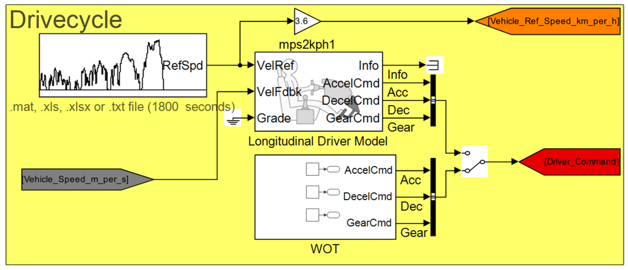
For the simulation, we used a WLTP (Worldwide Harmonized Light-Duty Vehicles Test Procedure) driving cycle, which better represents real traffic conditions. For comparative simulations, the NEDC (New European Driving Cycle) or a self-made drive cycle can also be suitable; however, when testing the model, we found that several large accelerations and decelerations highlighted differences [39]. The NEDC was introduced by the European Union on 1 July 1992, and it is no longer sufficiently up to date for a representative mapping of individual daily car use. The WLTP is a globally harmonized measurement procedure for passenger cars and light commercial vehicles, which from 1 September 2017 provides more realistic fuel consumption values with much more dynamic test parameters. The main differences are that the NEDC test lasts 20 min, while according to the WLTP protocol, the car must be tested for 30 min. The measuring distance is 11 km in the former and 23.25 km in the latter. The NEDC consists of two cycles, while the WLTP consists of four, with transitions between city and highway driving. In the case of the NEDC, the maximum speed during the measurement is 120 km per hour; for the WLTP, it is 131.

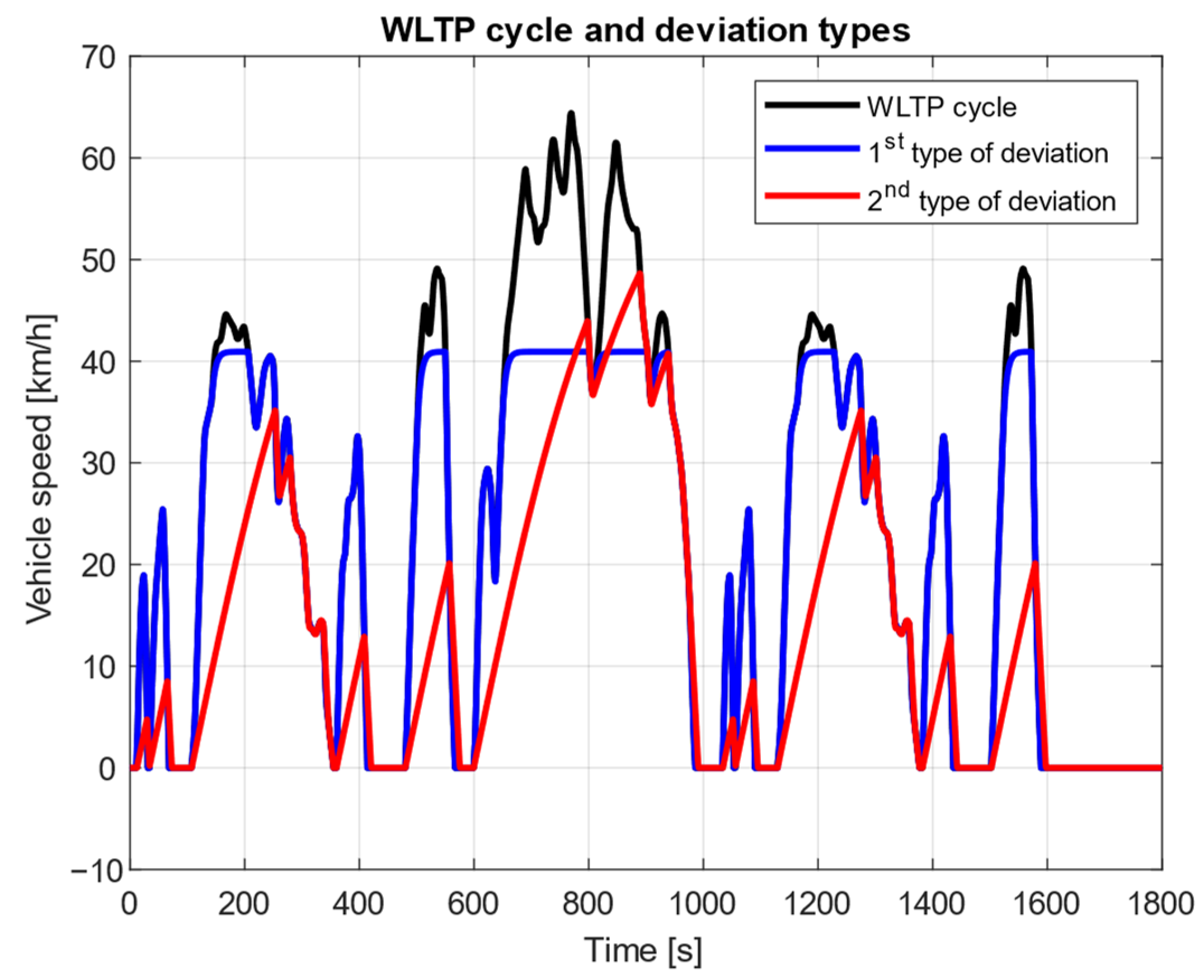
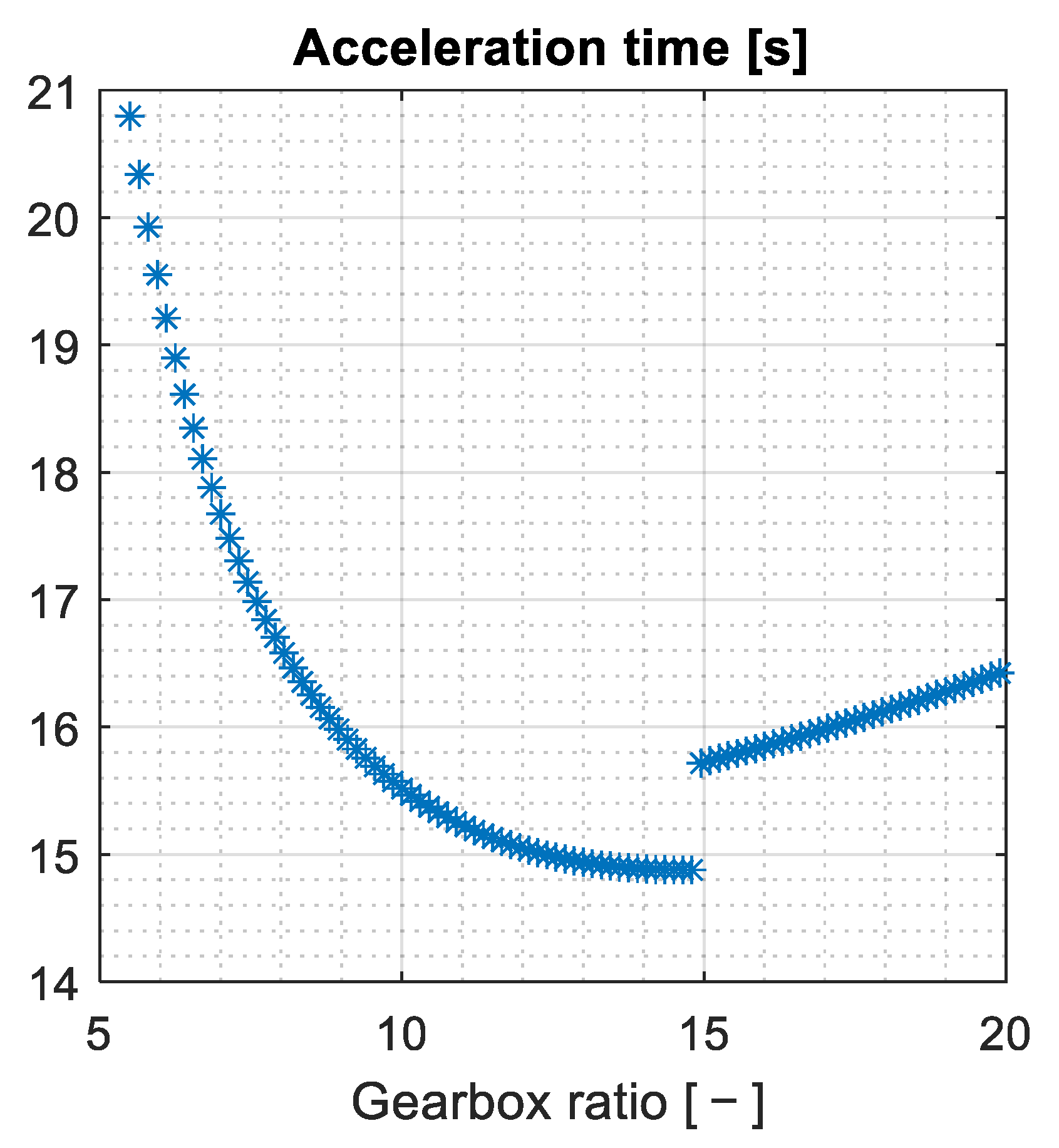
There are two types of deviations between the driving cycle and the actual vehicle speed. In the case of the first type of deviation, with the given gear ratio, the power of the engine is not sufficient to reach the maximum speed of the driving cycle, so the top speed of the vehicle is maximized at the working point when the traction force and all resistance forces are balanced. In the case of the second type of deviation, the driving torque/braking torque generated on the vehicle’s wheels with the given gear ratio is insufficient to create the required acceleration/deceleration in the driving cycle. The applied WLTP cycle with these two types of deviations is shown in Figure 4. In the first type of deviation, we find that the vehicle model is not able to reach the top speed in the driving cycle. This can be considered as the vehicle being “weak”. A physical vehicle has normal acceleration because “weak” vehicles are hard to sell. In the case of a model with realistic parameterization, this usually results from a modeling error. In the second type of error, it can be seen that the vehicle “falls behind” in the driving cycle. This may be due to slow control or a non-ideal gearbox ratio. As a result, sufficient traction cannot be generated on the wheels. If the effect of the gear ratio is examined, too large a ratio causes the first type of difference, while too small a ratio causes the second type of difference.

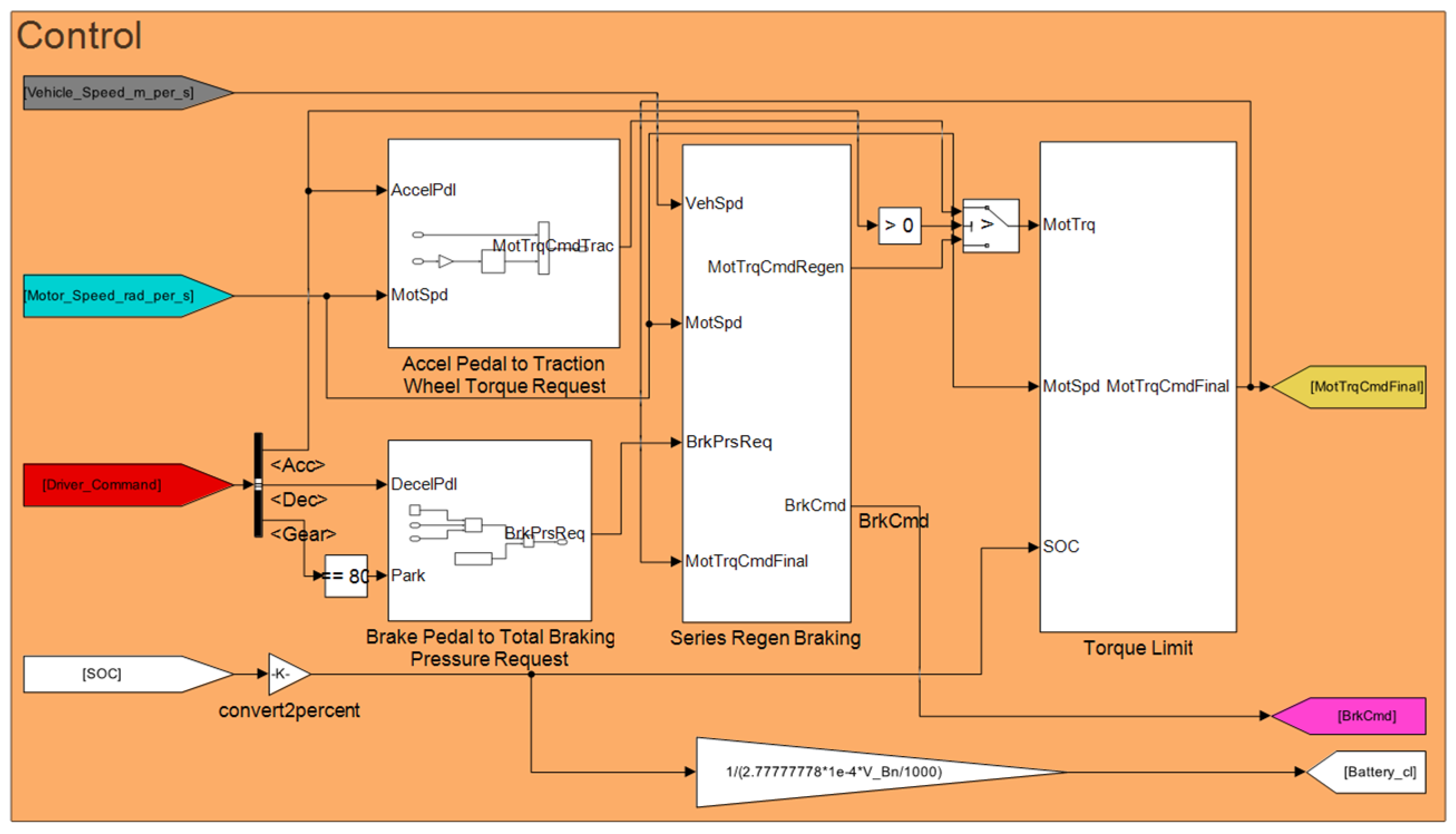
2.3. Control

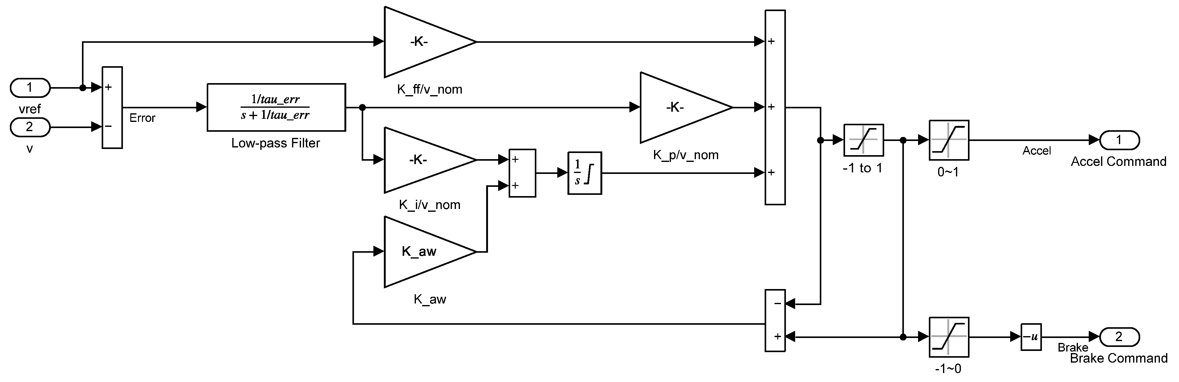
The driver is a PI controller, as can be seen in Figure 5. The input values of the controller are the reference speed from the drive cycle, the real speed of the vehicle, and the rate of climb. The created control contains a low-pass filter to create a smoother error signal. The created signal has a saturation element that limits the signal from −1 to 1. Because of the saturation, the controller has an anti-windup function as well. After this, the signal was separated into an acceleration command (from 0 to 1) and a brake command (from −1 to 0). The brake command will be separated with another block into brake pressure and generator regenerative braking.

The driving cycle does not include a hill, but the model can simulate its effect if required. As mentioned before, the output value is an accelerator pedal position between 0 and +1 and a brake pedal position between 0 and −1. Together with the speed of the vehicle, these outputs are the input of the engine controller, which gives the desired torque to the output signal, taking on a positive or negative value depending on whether it is necessary to accelerate or brake with recuperation. The control ensures in a way that the vehicle is recuperating as much energy as possible.

2.4. Framework Structure

The goal is to create a flexible framework that is suitable for the cooperation and division of work between several research groups. The effect of changing various parameters in the planning phase can be quickly analyzed. The parameters can be modified, varied, and selected freely. Various parameter sensitivity tests can also be performed. Ultimately, it can also be used for optimization. In general, it can be said that both researchers and manufacturers try to minimize consumption. The goal is to create the framework in such a way that we could optimize an arbitrary output, or, if appropriate, perform a multi-objective optimization by weighting several output values. Even with this simplified model, there are several input values that cannot be modified independently because they affect the values of other parameters. An example is battery capacity. An increase in the battery capacity can be achieved in practice by increasing the number of cell lines connected in parallel. This results in a decrease in the internal resistance of the battery. A similar approach was taken with the vehicle weight, where the total weight of the vehicle increases in direct proportion to the increase in battery capacity. This was taken into account with a constant energy density of 180 Wh/kg. In practice, the encapsulation of the battery can break this linearity to some extent, but it does not change in terms of its nature. If a given variable of the model is coupled to other variables, then the framework does not change it directly, only indirectly through the coupled variables. If a given variable of the model is not coupled to other variables, it is important that the coupling must take place outside of the framework.

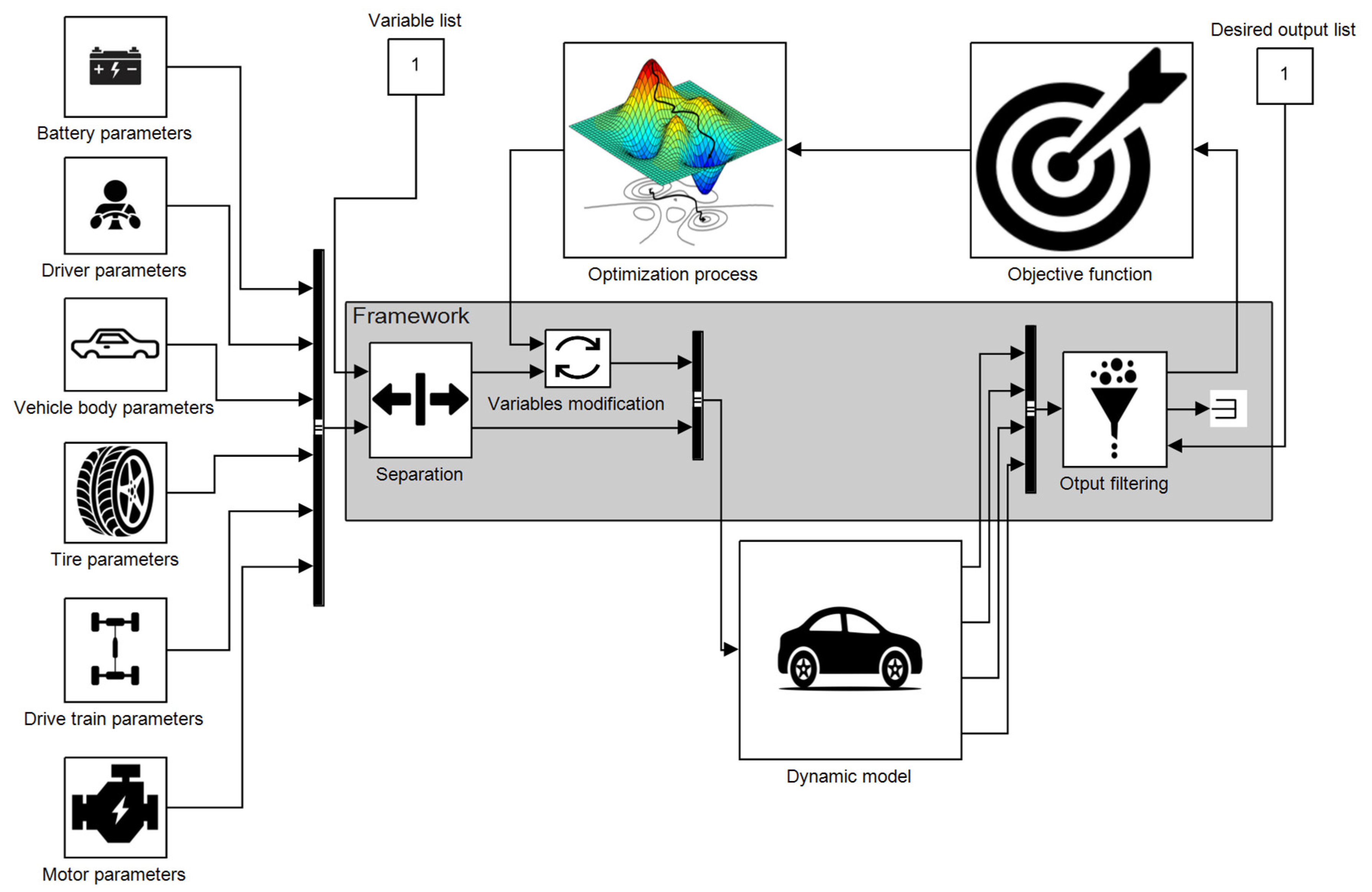
For the above reasons, the couplings were not changed and their analysis was not carried out, and we recommend using the framework only to modify input variables and read arbitrary outputs. Furthermore, it had to be created in a way that optimization could be run even when changing several parameters at the same time. To avoid having to rewrite the program lines of the entire framework to modify the parameters or their quantities, the names and values of the variables to be modified must be specified in a cell array variable. Here, the first column is the variable names stored in strings, and the second column is the values of the variables. It is sufficient to enter the last value of the distance traveled by integrating the speed as the return value. However, testing, optimization, and simulation verification may require the entire time-continuous signal. It follows that we need a function that can give scalars, vectors, and matrices as an output. From this point of view, the output value is also a cell array. Since this research was carried out within the framework of research activity involving several research groups, the framework had to be created in such a way that other research groups could optimize it with simpler, more transparent modifications. This entails that what we create as a framework must be embedded in the objective function used for optimization, which performs the necessary conversions. With this solution, research groups can work together in such a way that both the simulation model and the optimization procedures remain modular. The graphical structure of the created framework is shown in Figure 6. The created code with comments is shown in Appendix A.

This figure is an example of the application of the created framework for optimization tasks. Optimization algorithms call for an objective function. The input of this objective function is the modified input data, and the output returns the output parameter to be optimized. This output parameter is evaluated by the optimization algorithm. Since the framework is created as a function, the objective functions of any optimization algorithm can be used arbitrarily. If the goal is multi-objective optimization, then this framework can be embedded in another function to generate a weighted objective function from the outputs. Without such a modular framework, if it becomes necessary to modify the objective function; then, a structural transformation of the basic model may often become necessary. The left side of the figure contains the model parameters that can be flexibly modified. The input of the created framework is the list of parameters and its values that shall be modified. The variables from the parameter list are selected by the separation process. In the next step, the simulation is executed with the modified variables and static parameters. The simulation outputs can be filtered as demanded too. Due to the flexible selection of inputs and outputs, an arbitrary mapping function can be created.

The created framework function is an ${\mathbb{R}}^n\to {\mathbb{R}}^m$ MATLAB function. This creates the mapping between the model inputs and outputs. Since the values of $n$ and $m$ can be flexibly modified, other research groups can create task-specific objective functions.

3. Results

In this section, some applications of the framework are presented. Section 3.1 briefly describes the implementation of the framework and the electric motor efficiency map used in the testing. Section 3.2 then describes the Simscape vehicle model and the sensitivity test on the driving cycle presented above. Section 3.3 presents further tested application examples, where the sensitivity test of the Simscape vehicle model presented above and a Simulink Powertrain Blockset vehicle model from 0 to 100 km/h is performed. Since the aim of this research is to present a framework behind which the model used can be changed at will, our goal is not to validate the model.

3.1. Implementation of the Framework

As mentioned earlier, the input and output values of the created target function must be specified in a cell array-type variable. For later optimization, it is advisable not to set the efficiency of the electric motor to a constant value, but to enter it in a speed-torque field. This so-called efficiency map must be provided per data point. To allow for changing the performance of the motor, these efficiency values must be updated correctly. More information can be found about the motor data creation in [19].

The efficiency map is shown in Figure 7. Since a vehicle has acceleration and deceleration phases in both forward and reverse during everyday use, it is necessary to indicate all four quadrants on the efficiency map.

3.2. Testing the Framework, Sensitivity

During the testing, we performed a sensitivity test in a script, during which we modified the ratio of the final drive and monitored the energy consumption. In order to be sure of the correctness of the results, we measured not only the charge change of the battery but also the electrical work of the motor. Due to the internal resistance of the battery, the work calculated for the motor is smaller but proportional to all simulated values. Since the controller is based on the difference between the desired and the actual speed, in cases where the final gear is too small, too much torque is applied to the motor, which causes the second type of difference between the speed prescribed by the driving cycle and the actual vehicle speed. Indirectly, the first type of deviation can also occur, since, in this case, the motor must operate at a higher speed because of the high gearbox ratio, and the power that can be extracted from the shaft is lower due to poor efficiency. The sensitivity test is shown in Figure 8.

3.3. Further Application Examples for the Framework

With the Simscape model presented above, a data set was created by running a large simulation with the help of the framework, which was later used to create a replacement model for subsequent optimization. In order to consolidate the simulations, they were run independently on 12 identical computers. An algorithm running on the university’s computers called the framework with variable combinations randomly sampled from the design space and then collected them into a file. The data collection algorithm was started manually on all machines. In the case of a large computing capacity and larger machine parks, it may be worthwhile creating a computer cluster; however, given the size of the current problem, this was not justified. After combining the data, the data set was made available, which will be used in other research.

For 0–100 km/h acceleration, a sensitivity test was performed on the gear ratio function with the already presented Simscape model and another model created with Simulink Powertrain Blockset. The results of the Simscape model are shown in Figure 9. The two models do not model the same vehicle, so there are natural differences in the final results. These differences can also be found in the performance of the drive motor and in the modeling of wheel and drive chain dynamics. A sudden jump can be observed after the gear (14.8) for the minimum acceleration time. This phenomenon is observed due to the wheel model with a simple static/kinetic friction coefficient since, above this ratio, the wheel slips during acceleration. Below this gearbox ratio, wheelspin does not occur. This phenomenon occurs suddenly, and that is why there is a sudden jump in the diagram.

The used Simulink Powertrain Blockset model is shown in Figure 10 and its details in Figure 11, Figure 12, Figure 13, Figure 14 and Figure 15, and the results of the sensitivity test are shown in Figure 16. For transparency, the main units have been marked with the same background. In order to make the many blocks visible, these main units are presented individually. The “Goto” and “From” blocks included in the signal communication have the same color for the same signals.

The driving cycle part contains the WLTP cycle and the related driver model, as well as the Wide Open Throttle (WOT) block, which gives the controller a maximum gas pedal command. These two are switchable. This is shown in Figure 11.

The control part consists of four main units. The first two from the right generate the desired torque and brake pressure signals from the input data. The third breaks down the brake pressure signal into regenerative braking torque and a brake pedal signal. The block on the right limits the desired engine torque based on its performance. This is shown in Figure 12.

The battery and motor block contains the lookup table model of the battery, the DC-DC converter, and the lookup table model of the drive motor. Similar to the model used in Simscape, the motor model contains an efficiency map, which gives the motor efficiency according to the speed and torque point by point. This is shown in Figure 13.

The unit embodying the vehicle body contains the drive’s inertia, torsional dynamics, and wheel models. The difference between this model and the Simscape model is that the dynamics of the torsional stiffness of the drive are explained in more detail here, and the wheel model here uses the Magic formula. This is shown in Figure 14.

The output section enables the simulation to be integrated into the framework. The outputs are declared variables on the MATLAB Workspace interface with the name shown in the figure. These variables are concatenated by the framework into a single output, as described above. This is shown in Figure 15.

As the wheel model contains the Magic formula used in the Simulink model, there is a gradual increase after the gear ratio corresponding to the minimum acceleration time. The randomly occurring outliers are due to the more complex wheel model, since here the choice of the automatic step interval of the solver has a small, but negligible, effect on the final result.

4. Discussion

In this paper, our approach to creating a framework was presented through dynamics simulation of an electric vehicle. The potential areas of application were described, and finally, an example of a sensitivity test was also presented for application. The created framework provides an opportunity for simple collaboration between different research groups, as it provides an interface between them. Our future goal is to further generalize and test the created framework in order to provide an application-independent solution for similar cases when the effective cooperation of research groups is made difficult by the separation of specialist areas. The goal is to implement a framework that can easily be applied to other software environments and tasks without significantly affecting computational efficiency or degrading the scalability of the model.