Analysis of the Accuracy of CAD Modeling in Engineering and Medical Industries Based on Measurement Data Using Reverse Engineering Methods

Abstract

The reverse engineering (RE) process is often necessary in today’s engineering and medical industries. Expertise in measurement technology, data processing, and CAD modeling is required to ensure accurate reconstruction of an object’s geometry. However, errors are generated at every stage of geometric reconstruction, affecting the dimensional and geometric accuracy of the final 3D-CAD model. In this article, the geometry of reconstructed models was measured using contact and optical methods. The measurement data representing 2D profiles, 3D point clouds, and 2D images acquired in the reconstruction process were saved to a stereolithography (STL) model. The reconstructed models were then subjected to a CAD modeling process, and the accuracy of the parametric modeling was evaluated by comparing the 3D-CAD model to the 3D-STL model. Based on the results, the model used for clamping and positioning parts to perform the machining process and the connecting rod provided the most accurate mapping errors. These models represented deviations within ±0.02 mm and ±0.05 mm. The accuracy of CAD modeling for the turbine blade model and the pelvis part was comparable, presenting deviations within ±0.1 mm. However, the helical gear and the femur models showed the highest deviations of about ±0.2 mm. The procedures presented in the article specify the methods and resolution of the measurement systems and suggest CAD modeling strategies to minimize reconstruction errors. These results can be used as a starting point for further tests to optimize CAD modeling procedures based on the obtained measurement data.

1. Introduction

The manual measurement of free surfaces is almost impossible due to the inability to obtain enough measurement data to describe a given feature of the measured geometry. However, the remarkable advancements in the computerization of measurement systems and their integration with computer-aided design (CAD) systems have resolved this issue [1,2,3]. This led to the development of coordinate measuring methods that allow the digitization of geometries optically [4,5] and via contact [6,7]. The results of these processes are digital data in the form of measurement points with coordinates usually expressed in the global coordinate system of the measuring machine. It is also possible to obtain digital data from 2D images obtained with computer tomography (CT) [8,9] or magnetic resonance imaging (MRI) [10]. The development of contact and optical coordinate measuring systems has contributed to optimizing production by reducing the time consumption of measurement procedures, increasing the accuracy and repeatability of measurements, and eliminating errors caused by human factors [11].

Coordinating measuring is also crucial in reverse engineering (RE) [12,13]. The task of RE is to convert an existing object into its digital form e.g., through a stereolithography (STL) file, which in turn provides the basis for further work by designers and computer analysists using CAD systems [14]. Through RE methods, it is possible to reconstruct this information based on an existing object that does not have technological or construction documentation. The RE process is most often used in the automotive [15,16], aerospace [17,18], or archaeological [19,20] industries. It is also very often used in medicine, for example, in the process of developing the geometry of anatomical structures [21,22], designing surgical instruments [23,24,25], or implants [26]. However, errors arise at each stage of the geometric reconstruction process [12,27]. Thus, equations are created between the actual model and the digital model. It is necessary to develop procedures at each stage of the reconstruction process to minimize the resulting differences. One of the critical aspects is selecting an appropriate measurement system that will allow the acquisition of the necessary amount of measurement data, which will enable the reconstruction of the object’s geometry in CAD at a later stage [28]. It is also essential to pay attention to the accuracy of the acquired measurement data. The accuracy of the reconstruction of the product geometry is influenced not only by the accuracy of the measurement system [5] but also by the adopted measurement strategy [6,28] and the quality of the measurement data processing [5,29,30]. The processing stage mainly involves filtering, combining, and positioning the measurement data [12,14]. The hybrid modeling process in the CAD system is also a crucial stage. It is most often associated with shape approximation involving spline curves and splaying of non-uniform rational B-spline (NURBS) surfaces, allowing a surface model to be obtained [22,29,31]. The last stage is usually a solid modeling process. The quality of the final 3D-CAD model obtained is mainly determined by the competence of the operator taking the measurements and the person processing the measurement data to obtain the 3D-CAD model. Researchers have conducted multiple studies to assess the accuracy of 3D-CAD model development based on acquired measurement data. These studies have mainly focused on testing the accuracy of measurement systems according to their relevant guidelines [32,33,34]. The tests have involved models created using additive and subtractive methods. Most often, the tests have been carried out on contact-based measurement systems such as coordinate measuring machines (CMMs) [35,36,37] and articulated-arm coordinate measuring machines (AACMMs) [38]. Additionally, research is being conducted on systems that use structured light [39,40,41] and laser light [42,43] to illuminate the model. In diagnostics, several studies have been carried out on tomographic measurement systems such as multi-detector computed tomography (MDCT) [44], cone beam computed tomography (CBCT) [45], and µCT [46,47].

However, there need to be more structured procedures that allow the reconstruction and development of a final 3D-CAD model using different methods and measurement data. Additionally, attention has yet to be given to the accuracy of the 3D-CAD modeling process based on the obtained measurement data. Considering this, this article analyzes a modeling process for 3D-STL models, whose geometries were obtained from measurements acquired using various coordinate measuring methods. This study selected models that are often used in the machining, aviation, and medical industries. Based on the developed 3D-CAD model, the process of evaluating the accuracy of CAD modeling was carried out. Knowledge of the errors in the obtained CAD modeling can, in the future, improve the reconstruction of geometries from data obtained using coordinate measurement systems.

2. Materials and Methods

One of the main steps in the RE process is obtaining information about the object’s geometric dimensions. These are obtained using contact or optical coordinate measuring systems. The presented research addresses the process of geometric reconstruction to develop 3D-CAD models for the following:

• a pulley based on measured 2D profiles;
• a model for clamping and positioning parts therein to perform the machining process, and a connecting rod based on a 3D point cloud obtained from a laser light scanner;
• a bevel gear and a turbine blade feather based on a three-dimensional point cloud obtained from a structured light scanner;
• the anatomical structures of the hip joint (femur and pelvic fragment) based on collected data represented as 2D images.

2.1. Geometric Reconstruction Based on Data Obtained Using the iNEXIV Optical System and MarSurf XC 20

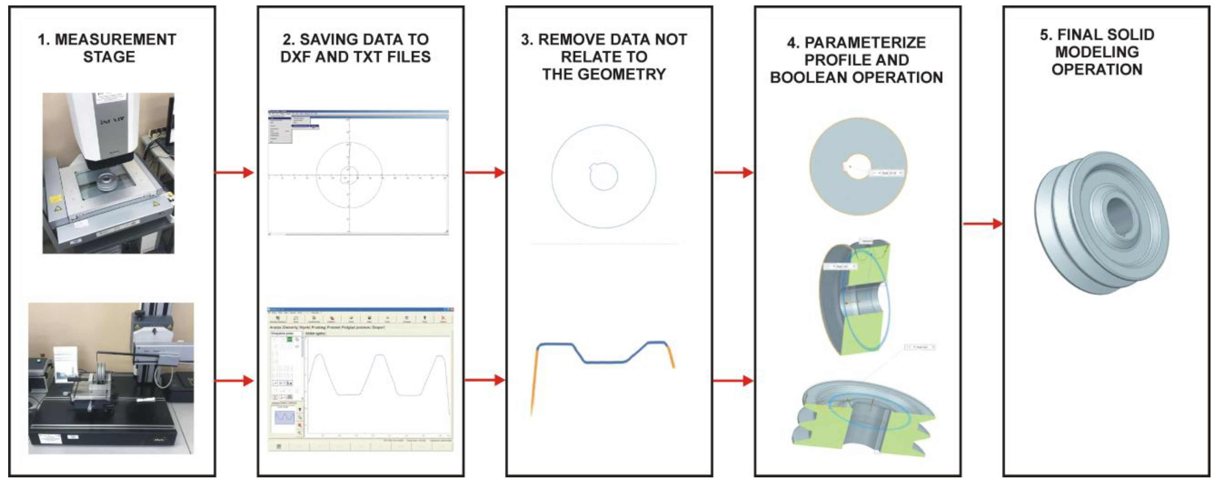
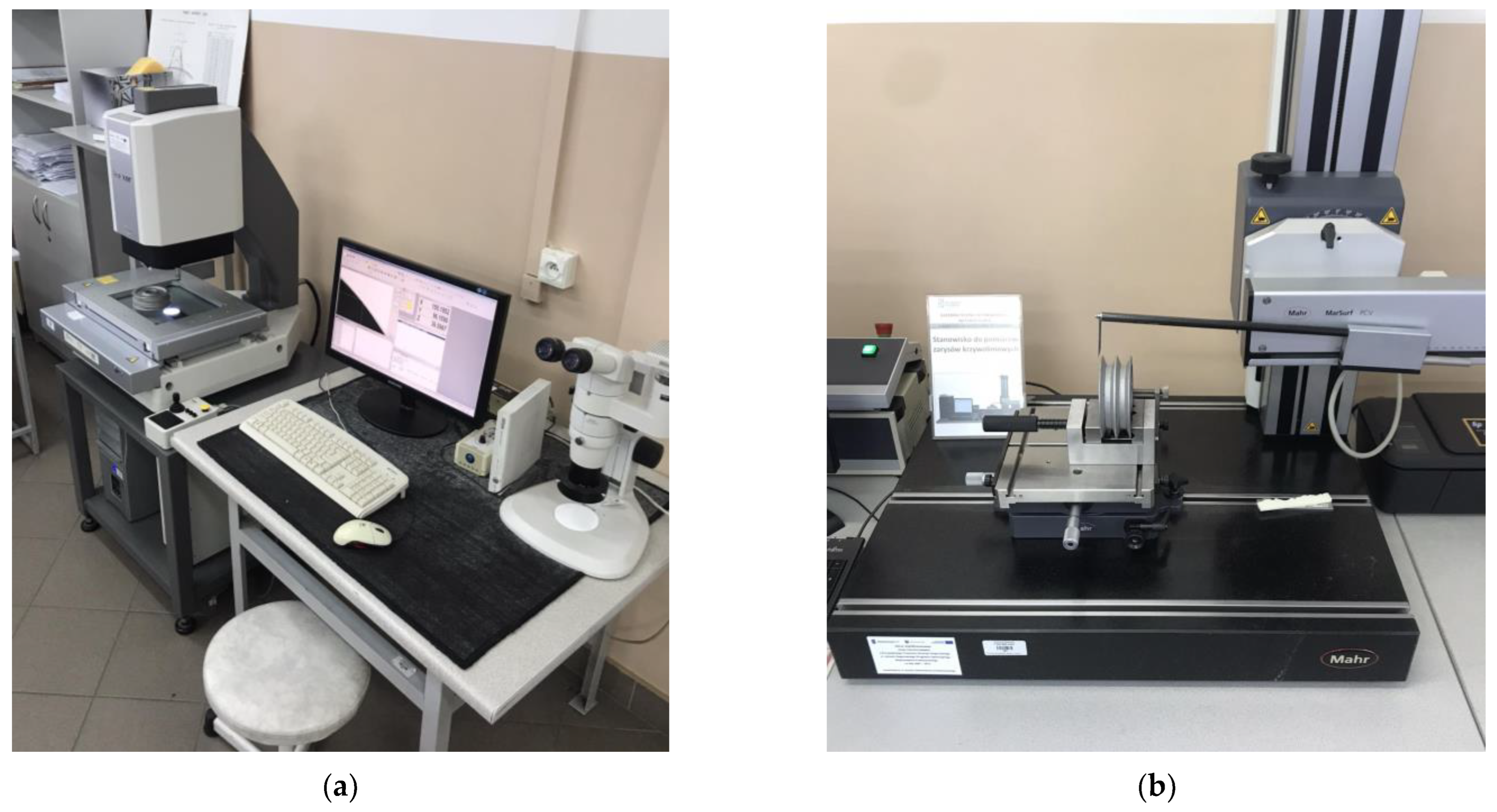
The process of reconstructing the geometry based on the obtained 2D profiles was carried out using the pulley model as an example. Using an iNEXIVE optical microscope, the measurements of the hub bore, splineway dimensions, and outer diameter were taken (Figure 1a). In the measurement process, the first step was to clean the pulley of any debris. The software for the microscope was launched, and the measuring table was set up with the wheel in the appropriate position. A binarized video preview and sharpened edges of the model’s geometric features were acquired to obtain accurate measurements. This was accomplished by adjusting the intensity of light incident on the object and the distance of the optical system from the measured geometry. The next step involved selecting three points on the hole’s perimeter to define the measurement section along which the geometry profiles were measured. The measurement resolution was also established, set at 0.02 mm for the pulley geometry. The 2D profiles were generated based on the measurements and then saved in drawing exchange format (DXF). The MarSurf XC20 was used to measure the shape of the pulley groove (Figure 1b). This device features advanced contour measurement technology for efficient and accurate profile measurement. The system consists of a measuring table and a tripod equipped with an arm and a measuring head. The measuring probe was selected based on the size and shape of the object to be measured, and moved along the measuring section in one plane, with the length of the section defined by the operator. The movements were controlled through special software on a computer. To perform the measurement, a dialog box defined the measurement segment and resolution, which in this case was 0.001 mm. The results were saved in 2D profiles in text (TXT) format.

Siemens NX software (version 2312) was used to reconstruct the pulley geometry. The first step was to load the measurement data obtained from an optical microscope. The data analysis started with reconstructing the pulley’s diameter using the Fit Curve function. For this, the Fit Circle option was selected from the dialog box, which fitted a circle to a set of points. The diameter of the pulley bore was reconstructed similarly. The dimensions of the splineway were parameterized using the Fit Line option. The Fit Curve and Fit Line functions were also used to develop the data collected on the MarSurf XC 20 system, allowing parameterization of the pulley and groove profiles. Once the profiles were developed, they were oriented to the corresponding planes in CAD system space and the traditional solid modeling process was carried out on them. The process involved extracting the sketches from measurements taken with an optical microscope using the Extrude function. Next, the previously created profile obtained with the MarSurf XC 20 was used to create the grooves of the pulley. The sketch was set on a plane passing through the center of the solid obtained in the previous step, and the Revolve function was used to create the grooves. A vector parallel to the axis of the pulley was selected as the vector of rotation, while the value of the angle of rotation was assumed to be 360°. The Boolean option Subtract was used to subtract the profile from the solid. The Mirror Feature function was used to select the second part of the solid, with the plane of mirroring being the plane passing through the center of the pulley, which at the same time was parallel to the face. After performing all the operations, a solid 3D-CAD pulley model was obtained and then exported to standard for the exchange of product (STEP) format.

2.2. Geometric Reconstruction Based on Data Obtained Using the Articulated-Arm Coordinate Measuring Machine MCA II with a Laser Head MMD×100

In this study, the process of reconstructing the geometry of a model for clamping and positioning parts in a machining process and a connecting rod was carried out based on an obtained 3D point cloud. The data representing the geometry of the models were acquired using the MCA II measuring-arm system with a mounted MMD×100 head, which illuminated the object with laser light. Using a beam of laser light to illuminate an object is a well-known technique for measuring objects. In this method, a beam of laser light is deflected by a mirror towards the scanned model. The beam is then scattered on the object’s surface, and the camera records its position. This method is suitable for short-range measurements because the accuracy of the measurement is inversely proportional to the distance of the laser from the scanned model. Before taking any measurements, the components were coated with an anti-reflective spray to prevent laser light from reflecting off their surfaces. The scanning process was carried out in various stages, each involving scanning the models for clamping and positioning parts for a machining process (Figure 2a) and a connecting rod (Figure 2b) from different angles to obtain comprehensive geometric information with the applied maximum resolution of point clouds set to 0.01 mm. The outcome of the measurement process was a three-dimensional point cloud that mapped out the models’ geometry, which was saved in STL format. Next, any noise and software errors in the triangle mesh created during the measurement were removed. Lastly, the 3D-STL models underwent a CAD modeling process using Siemens NX software.

The process of CAD modeling of the geometry of the equipment used for clamping and positioning parts in the machining process consisted of several steps. In the first step, the Section Curve function was used. This allowed the generation of planes to intersect the model, onto which measurement points defining the basic dimensions of the geometry were then projected. With the obtained points, it was possible to create sketches. The next step was to extract the elaborated sketches using the Extrude function. Thus, the process of 3D-CAD geometric modeling began with the development of the basic geometric dimensions of the model based on the sketches developed, ending with a section of the model defining the clamping directly. The developed solid model was exported to STEP format in the final step.

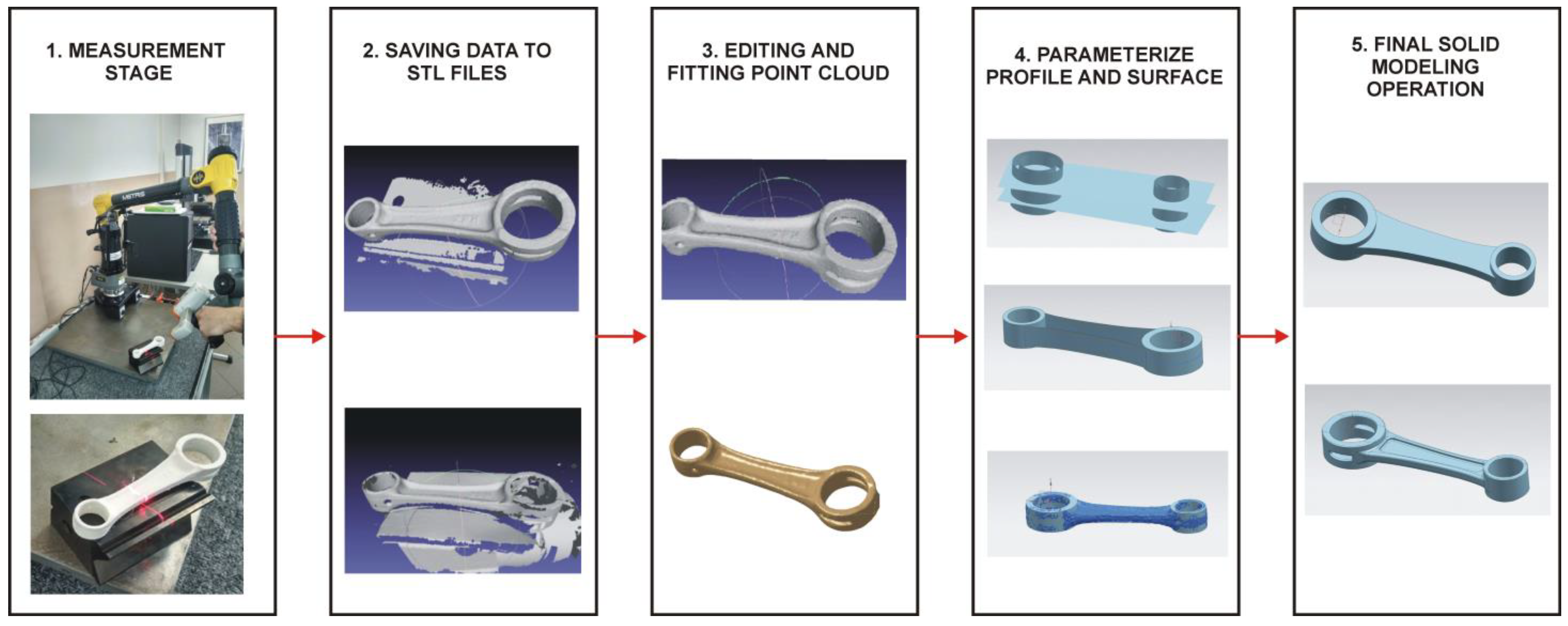
In the CAD modeling of the geometry of the connecting rod model, in the first stopper based on the Detect Primitives option, the basic areas defining planar and cylindrical surfaces were assigned to selected parts of the triangle mesh. Next, a median plane was defined onto which points mapping the outline of the side surface of the connecting rod were dropped. Curves were created based on the Fit Curve–Fit Spline option and then extruded. Thus, the side surfaces were defined. Its profile was also developed to select the top surface based on the projection of points on the plane. Based on the obtained points, curves were created using the Fit Spline and Fit Circle options. With the sketch fully parameterized, the missing surfaces were created. Each created surface was sewn together to create a fully described surface model, which was then saved into a solid model. The final step was to perform filleting and chamfering on the model. The solid model obtained in the final phase of the reconstruction process was exported to STEP format.

2.3. Geometric Reconstruction Based on Data Obtained from GOM Scan 1 Structured Light Scanner

The process of geometric reconstruction based on the obtained three-dimensional point cloud was carried out using the examples of a model of a helical gear and a turbine blade. The data representing the three-dimensional point cloud were acquired using a GOM Scan 1 scanner (Figure 3). The system illuminated the object with a structured light to make measurements. It was equipped with a measurement head mounted on a tripod, allowing the head’s appropriate height and angle to be set relative to the object on the rotary table. In the case of methods that illuminate the object with structured light, information about the entire surface of the measured object is obtained from measurements based on Gray’s stripe projection. A specific raster is projected onto the surface of the measured object. A prerequisite for correct measurement is good visibility of the stripes on the surface of the workpiece. The non-contact coordinate measuring system works with a rotary table and GOM Inspect software (version 2021). In our study, first of all, the calibration process of the GOM Scan 1 measuring system was carried out. To carry out the measurements, it was necessary to check, among other things, the exposure time, the alignment of the measuring head in relation to the plane of the object to be measured, the number of markers on the geometry, and the reflectivity of the object surface. In addition, where a rotary table was used, it was also necessary to determine the number of its angular settings during geometric measurement. A matting agent was applied to the models’ surfaces to prepare them for scanning and to minimize light reflection. Additionally, several reference points were attached to the models to define their initial position and orientation in space. This ensured greater repeatability, thus reducing the impact of systematic and random errors when digitizing the geometry. The measurement was carried out with the highest possible resolution, 0.01 mm. Finally, the measurement process resulted in a three-dimensional point cloud that mapped the geometry of the models, which was saved in STL format. The obtained triangle mesh underwent further processing, and CAD modeling was performed using Siemens NX software. First, a preliminary analysis of the triangle mesh was conducted. Based on this analysis, the noise created during the measurement process was removed.

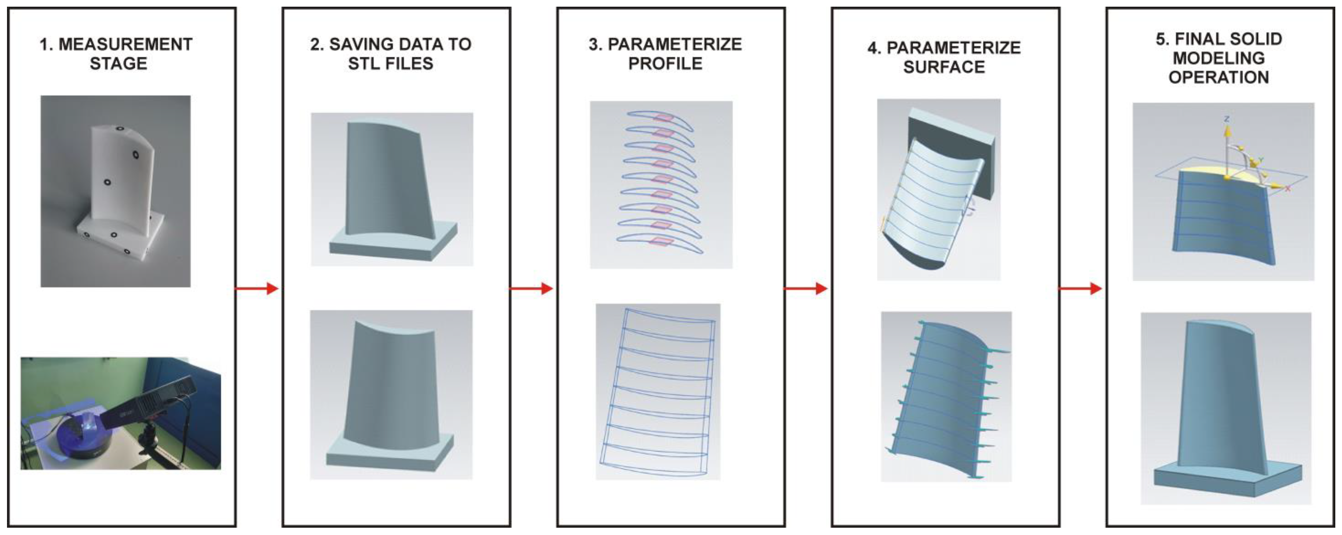
The CAD modeling of the turbine blade geometry consisted of several steps. In the first step, it was necessary to define the plane using the “Datum Plane” tool. In the next step, sections were generated on the surface of the 3D-STL model using the “Section Curve” tool. The operation was duplicated, obtaining nine sections of the blade. Points were projected on the obtained section planes. The “Fit Curve” tool was used to join the points. Each parameterized profile consisted of four curves. The convex and concave parts of the blade, as well as the edge of attack and trailing edge, were modeled separately. The curves in the subsequent sections were created similarly. To avoid the phenomenon of surface waviness and to obtain a more accurate representation of the turbine blade, guide curves were created using the “Studio Spline” tool. Next, surface patches were spanned on the created curves. For this purpose, the “Through Curve Mesh” command was used. The surface model was converted into a solid model and exported to STEP format in the next step.

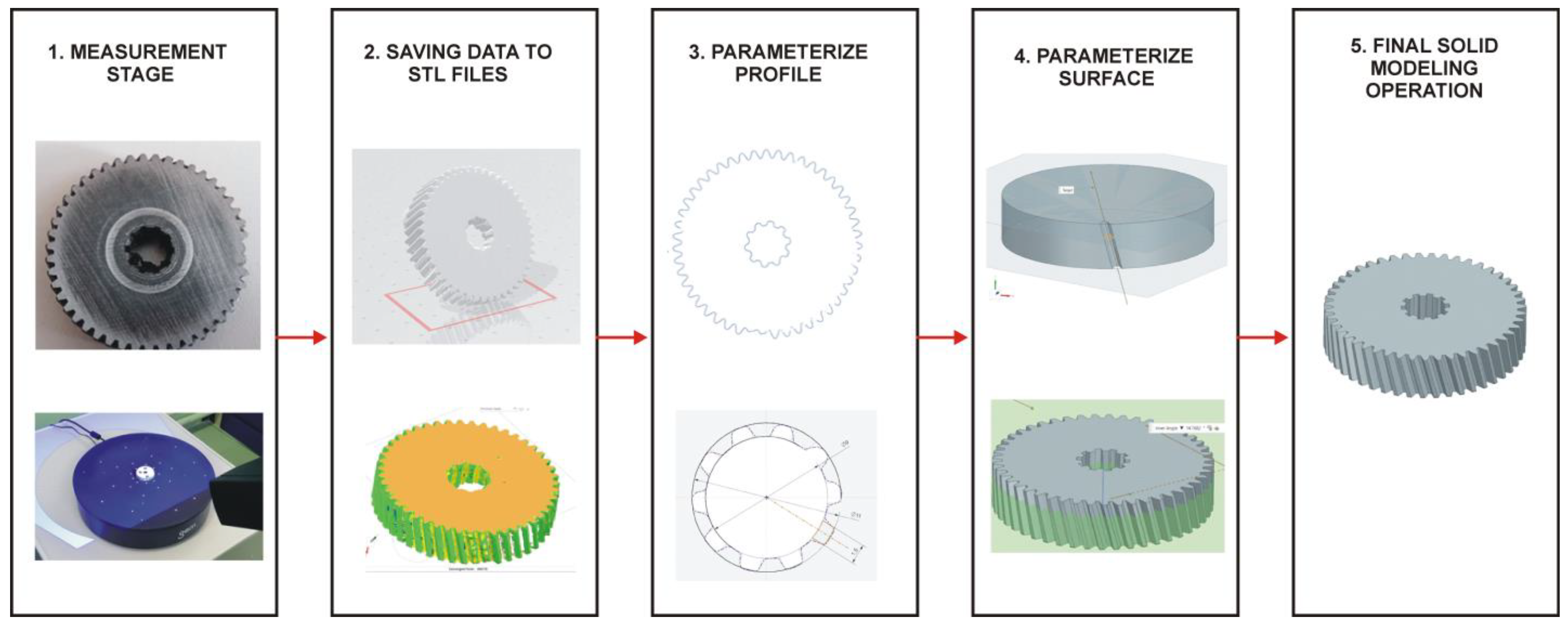
The CAD modeling of the helical gear geometry consisted of several steps. The first step was to reconstruct the contour of the functional surface and spline. In the NX environment, the Section Curve function was used. This function defines a curve that represents a cross-section through a three-dimensional object. The Fit Curve function in the program was used to create parameterized curves for a set of points. The vertices of the tooth heads were selected as the fit points, thus obtaining the first circle. Similarly, a second circle was created based on points at the teeth’s feet. By approximating the sets of points, a tip diameter and a root diameter of the gear were obtained. With the Extrude function, a solid representation of the diameter was extruded. The Fit Curve function was again used to make teeth on the elaborated solid. Based on the Fit Spline option, curves were fitted to the acquired point cloud to develop a tooth space. Surfaces were spanned on the fitted curves to develop the side surface of the tooth using the Fit Surface option. The prepared sketches, surfaces, and vectors parallel to the edge of the plane were selected. The result was a ray that was the path of the notch drawing. The program selected the solid by default and cut the material from it to form the notch. The next step was to work out the rest of the teeth similarly. The solid model obtained in the last phase of the process reconstruction was exported to STEP format.

2.4. Geometric Reconstruction Based on Data Acquired with a Multi-Slice Computed Tomography (CT) Scanner

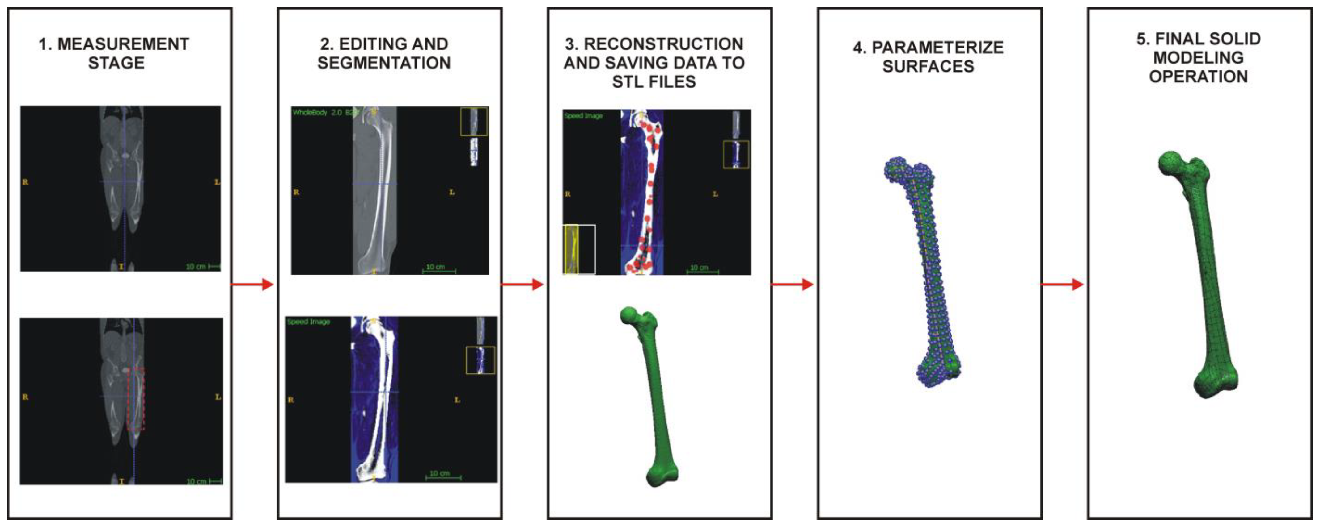
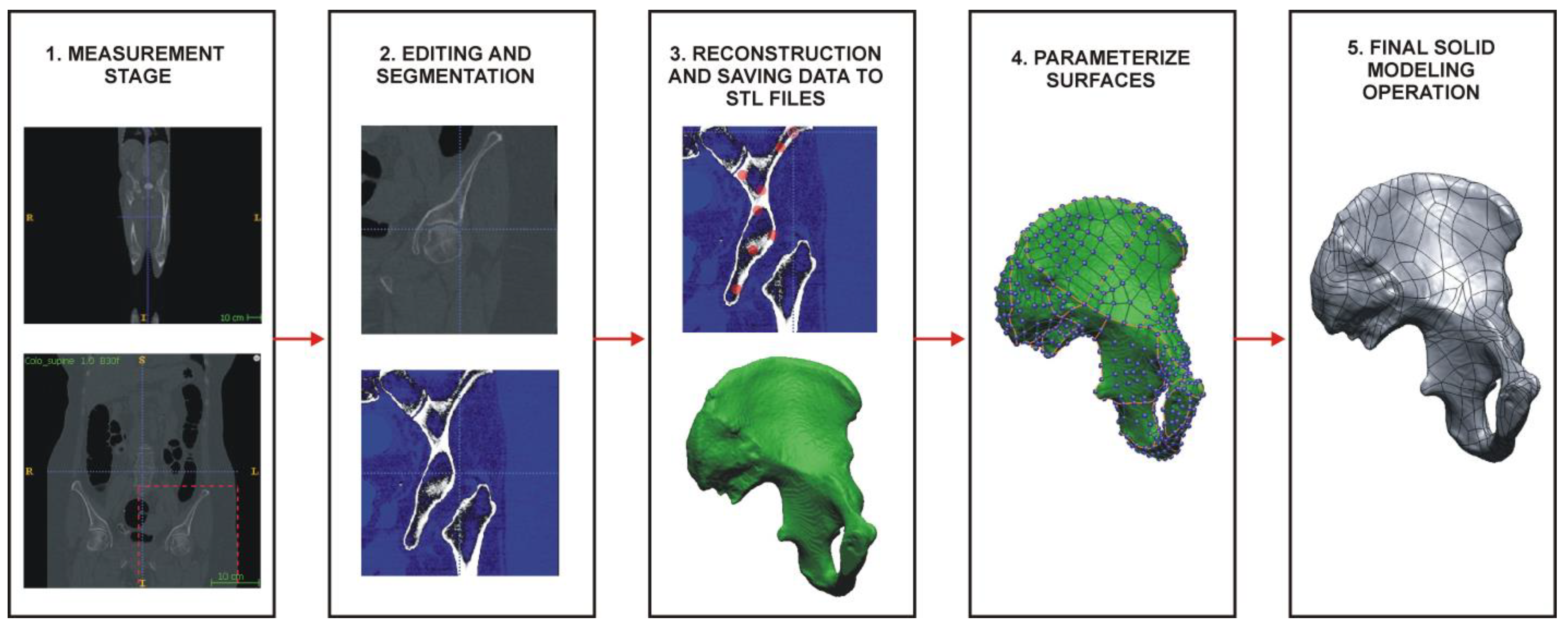
The first stage of reconstructing bone structures representing a fragment of the pelvis and the femur consisted of obtaining Digital Imaging and Communications in Medicine (DICOM) measurement data. The research was conducted on a patient scanned on a Siemens Somatom Definition AS+ multi-slice tomography scanner. A traditional scanning protocol for the hip joint area was used during the measurement process. The obtained volumetric data were characterized by an anisotropic voxel structure: 0.4 mm × 0.4 mm × 0.7 mm. The ITK-SNAP program performed the numerical processing of DICOM data and geometric reconstruction. Segmentation of bone structures in the hip joint area was performed using the thresholding method based on the collected DICOM data, which belongs to the area method group, involving selecting pixels with a similar shade and classifying them into one group defining a given tissue. In segmenting the bone structures of the pelvic fragment and the femur, a lower threshold value of 200 HU was selected. On the set of 2D contours created as a result of the segmentation process, the process of reconstructing the 3D geometry of the bone structures was carried out. The reconstruction process used the isosurface, which is a type of surface rendering method based on the marching cube algorithm. Due to the presence of disproportionate triangles in the resulting 3D-STL model, a surface editing process was carried out, which involved creating a triangle mesh consisting of more regular triangles. Models prepared this way were saved to STL format and loaded into NX Siemens software. In the second stage, the CAD modeling process began. The same functions were applied to the model of the pelvic fragment and the femur. First, a mesh model of curves intersecting at right angles was developed. The developed curves were then dropped, through selecting Project Curve, on the surfaces of the 3D-STL models of anatomical structures. In the next step, parameterized surfaces were spanned on the curves that were projected onto the surface of the 3D-STL model using Rapid Surfacing. Because some surfaces on the 3D-STL models could not be automatically generated, a manual surface-filling process was carried out in some places. This was possible through moving the nodal points that determined the course of each dropped curve. Finally, the creation of surface models ended with covering the polygonal mesh with elementary NURBS-type surface patches. Each lobe, in addition to determining its boundaries through the dropped curve, was further described by a certain number of control points, determining the quality of the lobe’s fit to the corresponding section of the polygonal mesh. The surface model obtained in the last phase of the process was saved as a solid model and exported to STEP format.

3. Results

In the context of the information given in Section 2,

(a)

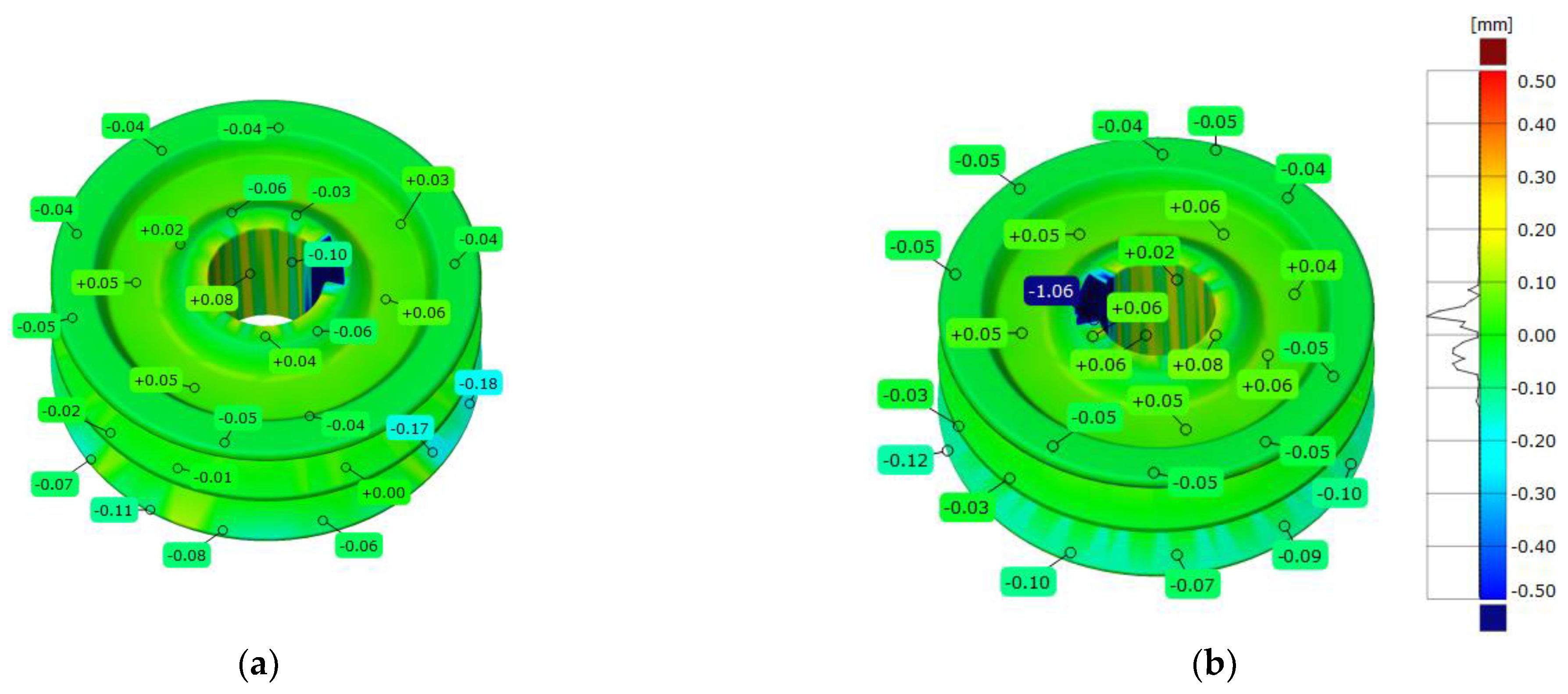
a pulley a CAD modeling methodology was developed (Figure 4), and three deviation map (Figure 5)

(b)

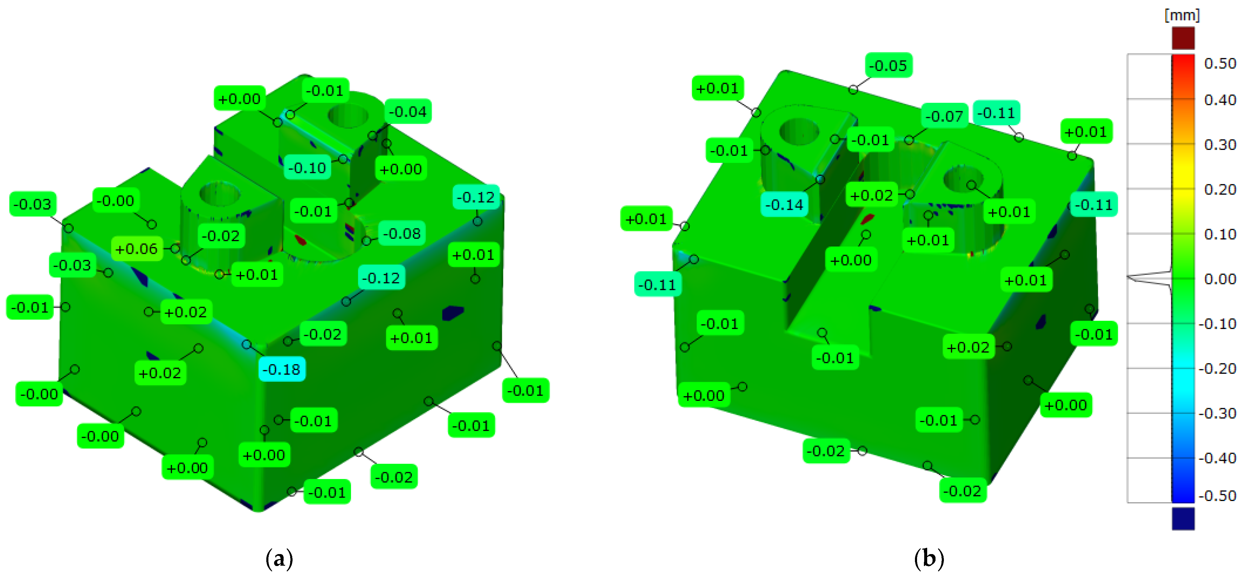
a model of parts used for clamping and positioning a CAD modeling methodology was developed (Figure 6), and three deviation map (Figure 7), and for a connecting rod a CAD modeling methodology was developed (Figure 8), and three deviation map (Figure 9)

(c)

a turbine blade a CAD modeling methodology was developed (Figure 10), and three deviation map (Figure 11), and for a helical gear a CAD modeling methodology was developed (Figure 12), and three deviation map (Figure 13)

(d)

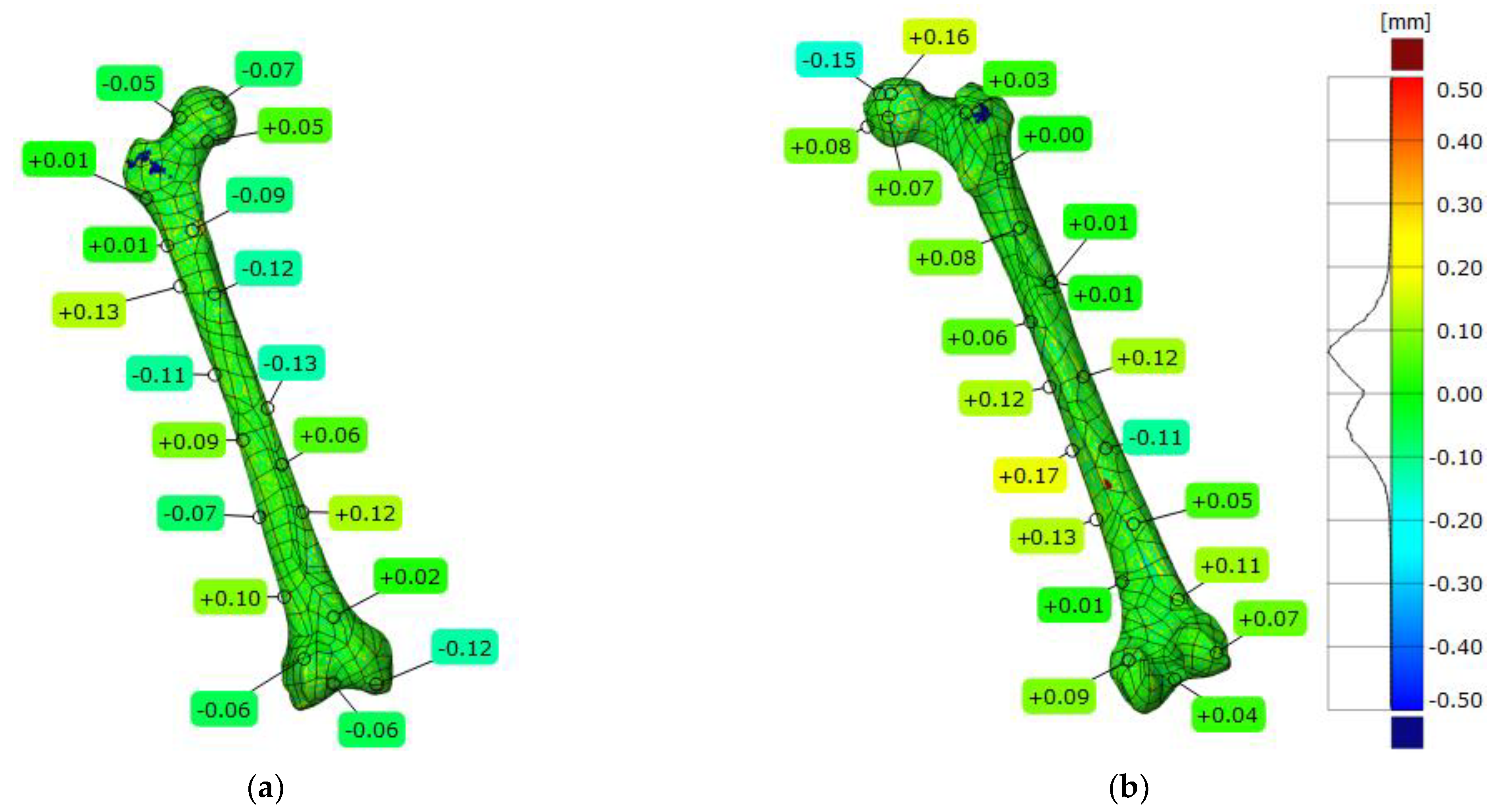
a femur a CAD modeling methodology was developed (Figure 14), and three deviation map (Figure 15), and for a pelvic part a CAD modeling methodology was developed (Figure 16), and three deviation map (Figure 17)

The process of verifying the accuracy of implementing the CAD modeling process was carried out using Focus Inspection and GOM Inspect software. The fitting of the nominal 3D-STL model obtained at the measurement stage and the reference 3D-CAD model generated at the design stage was performed using the best-fit method. This method is an iterative process that minimizes the square of the distance between two models. During implementation, the accuracy of the alignment must be about 0.005 mm. If the parameter value is larger, the process continues until the value is smaller. In addition, statistical data were developed in Table 1, Table 2, Table 3, Table 4, Table 5, Table 6 and Table 7 to define the maximum and minimum deviation values, range, mean, and standard deviation values.

Figure 4. Selected stages of pulley geometry reconstruction into a 3D-CAD model based on 2D profiles acquired during measurement.

Figure 4. Selected stages of pulley geometry reconstruction into a 3D-CAD model based on 2D profiles acquired during measurement.

Figure 5. Three-dimensional deviation map representing CAD modeling errors for a pulley model: (a) top view; (b) bottom view.

Figure 5. Three-dimensional deviation map representing CAD modeling errors for a pulley model: (a) top view; (b) bottom view.

Table 1. Statistical parameters representing CAD modeling errors for the pulley model.

Parameters	Pulley Model
Maximum deviation [mm]	0.278
Minimum deviation [mm]	−1.203
Range [mm]	1.481
Mean deviation [mm]	−0.002
Standard deviation [mm]	0.031

Table 1. Statistical parameters representing CAD modeling errors for the pulley model.

Parameters	Pulley Model
Maximum deviation [mm]	0.278
Minimum deviation [mm]	−1.203
Range [mm]	1.481
Mean deviation [mm]	−0.002
Standard deviation [mm]	0.031

Figure 6. Stages of reconstructing the geometry of a part used for clamping and positioning within a machining process, transformed into a 3D-CAD model based on the obtained 3D point cloud.

Figure 6. Stages of reconstructing the geometry of a part used for clamping and positioning within a machining process, transformed into a 3D-CAD model based on the obtained 3D point cloud.

Figure 7. Three-dimensional deviation map representing CAD modeling errors for in model of parts used for clamping and positioning within a machining process: (a) back view; (b) front view.

Figure 7. Three-dimensional deviation map representing CAD modeling errors for in model of parts used for clamping and positioning within a machining process: (a) back view; (b) front view.

Table 2. Statistical parameters representing CAD modeling errors for the model of parts used for clamping and positioning within a machining process.

Parameters	Model for Clamping and Positioning Part
Maximum deviation [mm]	0.161
Minimum deviation [mm]	−0.251
Range [mm]	0.411
Mean deviation [mm]	0.000
Standard deviation [mm]	0.009

Table 2. Statistical parameters representing CAD modeling errors for the model of parts used for clamping and positioning within a machining process.

Parameters	Model for Clamping and Positioning Part
Maximum deviation [mm]	0.161
Minimum deviation [mm]	−0.251
Range [mm]	0.411
Mean deviation [mm]	0.000
Standard deviation [mm]	0.009

Figure 8. Stages of reconstructing the geometry of the connecting rod into a 3D-CAD model based on the obtained 3D point cloud.

Figure 8. Stages of reconstructing the geometry of the connecting rod into a 3D-CAD model based on the obtained 3D point cloud.

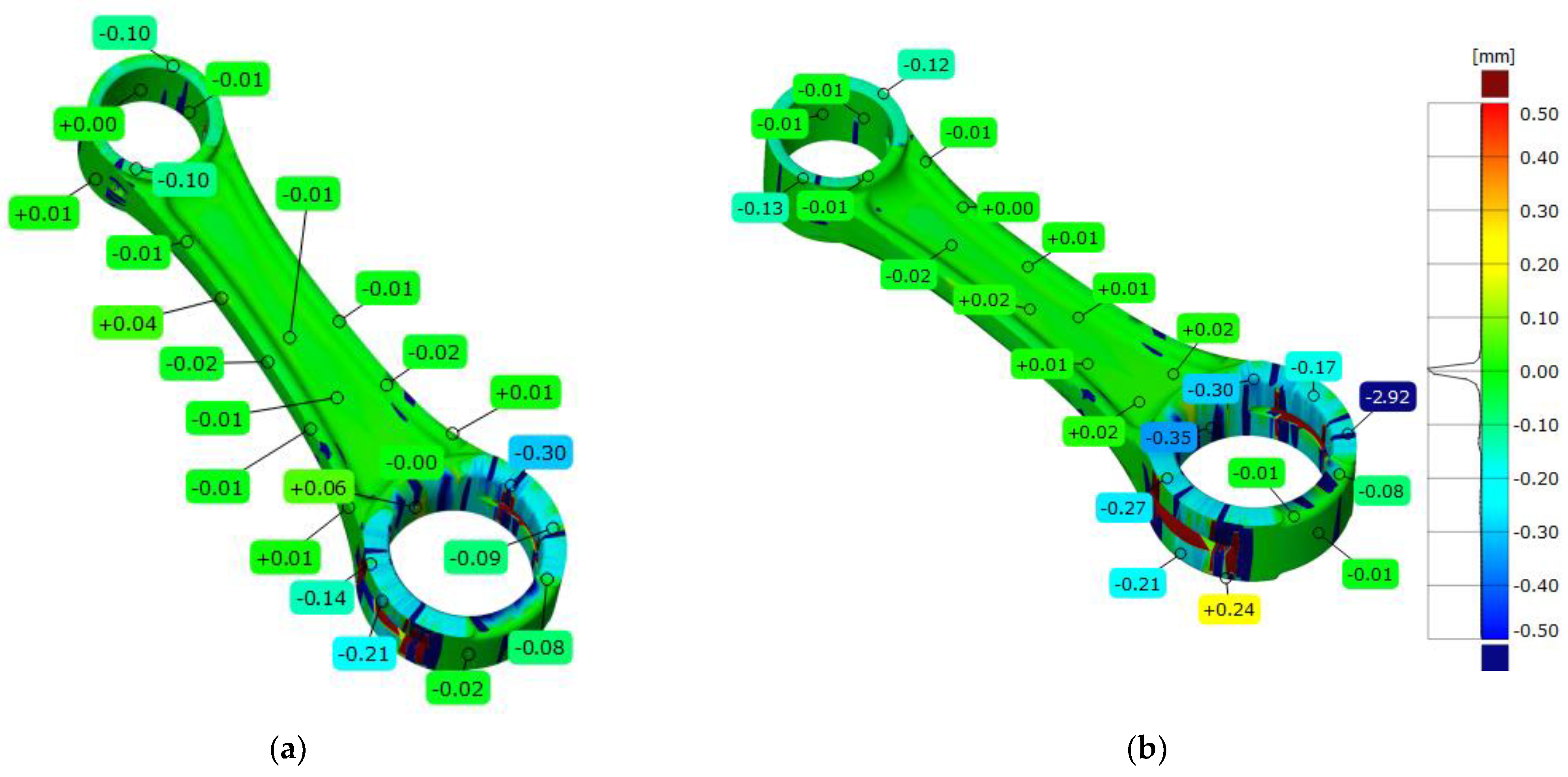
Figure 9. Three-dimensional deviation map representing CAD modeling errors for a connecting rod model: (a) top side view; (b) bottom side view.

Figure 9. Three-dimensional deviation map representing CAD modeling errors for a connecting rod model: (a) top side view; (b) bottom side view.

Table 3. Statistical parameters representing CAD modeling errors for the connecting rod model.

Parameters	Connecting Rod Model
Maximum deviation [mm]	0.223
Minimum deviation [mm]	−0.349
Range [mm]	0.571
Mean deviation [mm]	−0.003
Standard deviation [mm]	0.026

Table 3. Statistical parameters representing CAD modeling errors for the connecting rod model.

Parameters	Connecting Rod Model
Maximum deviation [mm]	0.223
Minimum deviation [mm]	−0.349
Range [mm]	0.571
Mean deviation [mm]	−0.003
Standard deviation [mm]	0.026

Figure 10. Stages of reconstructing the geometry of the turbine blade model into a 3D-CAD model based on the obtained 3D point cloud.

Figure 10. Stages of reconstructing the geometry of the turbine blade model into a 3D-CAD model based on the obtained 3D point cloud.

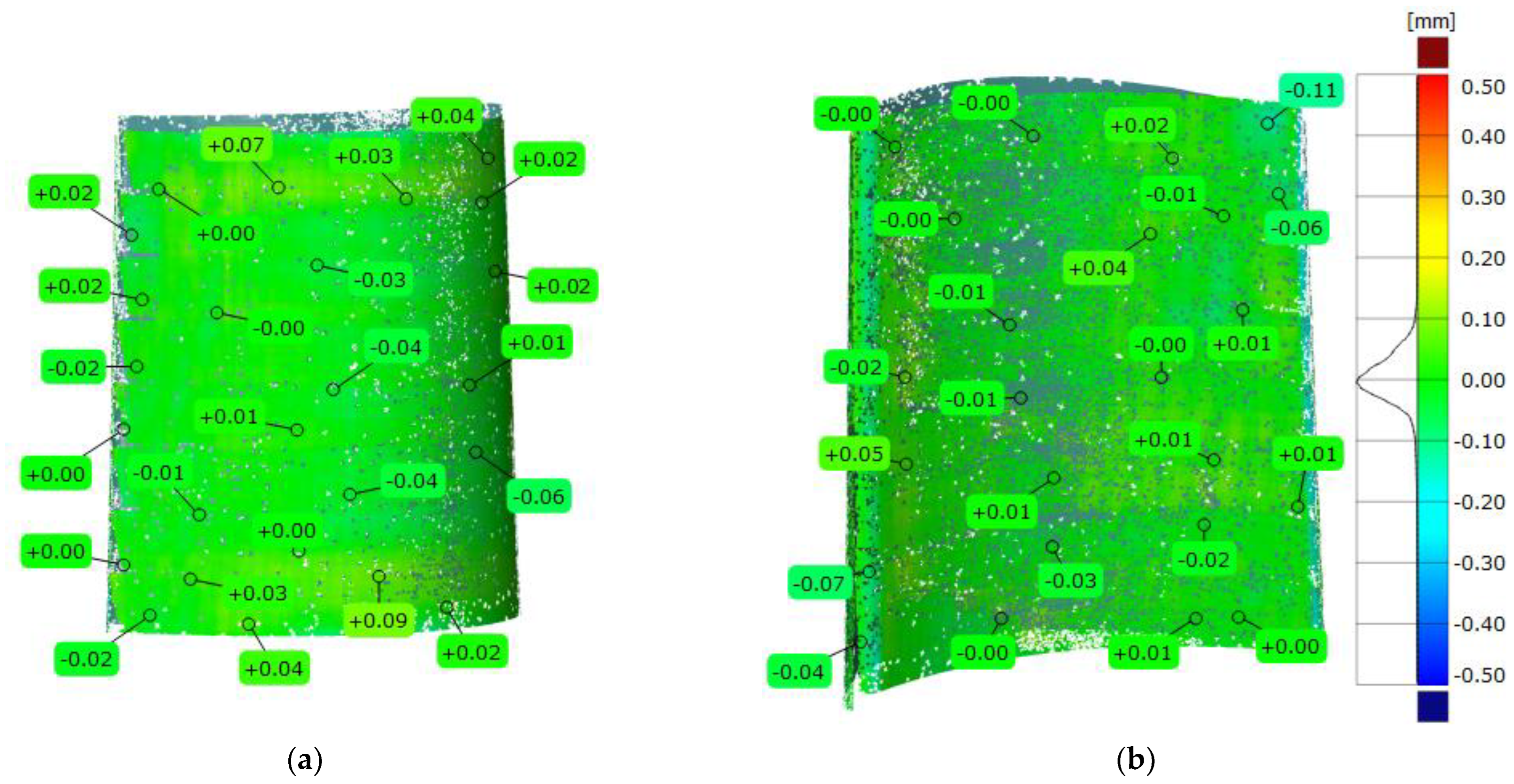
Figure 11. Three-dimensional deviation map representing CAD modeling errors for a turbine blade model: (a) convex side view; (b) concave side view.

Figure 11. Three-dimensional deviation map representing CAD modeling errors for a turbine blade model: (a) convex side view; (b) concave side view.

Table 4. Statistical parameters representing CAD modeling errors for the turbine blade model.

Parameters	Turbine Blade Model
Maximum deviation [mm]	0.686
Minimum deviation [mm]	−0.344
Range [mm]	1.030
Mean deviation [mm]	0.000
Standard deviation [mm]	0.045

Table 4. Statistical parameters representing CAD modeling errors for the turbine blade model.

Parameters	Turbine Blade Model
Maximum deviation [mm]	0.686
Minimum deviation [mm]	−0.344
Range [mm]	1.030
Mean deviation [mm]	0.000
Standard deviation [mm]	0.045

Figure 12. Stages of reconstructing the geometry of the helical gear model into a 3D-CAD model based on the obtained 3D point cloud.

Figure 12. Stages of reconstructing the geometry of the helical gear model into a 3D-CAD model based on the obtained 3D point cloud.

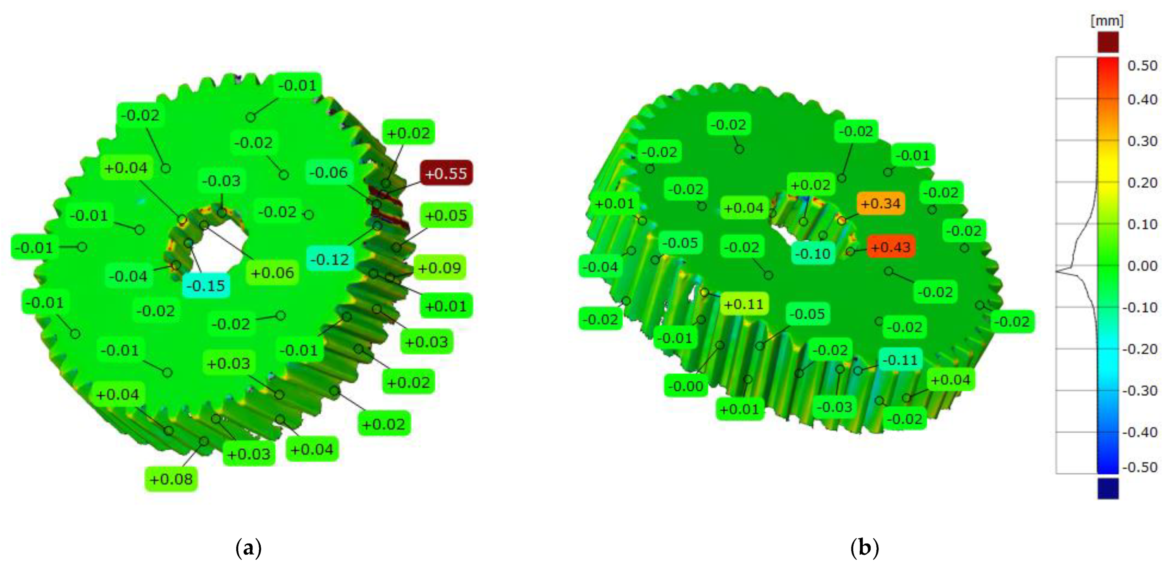
Figure 13. Three-dimensional deviation map representing CAD modeling errors for a helical gear model: (a) top view; (b) bottom view.

Figure 13. Three-dimensional deviation map representing CAD modeling errors for a helical gear model: (a) top view; (b) bottom view.

Table 5. Statistical parameters representing CAD modeling errors for the helical gear model.

Parameters	Helical Gear Model
Maximum deviation [mm]	0.693
Minimum deviation [mm]	−0.967
Range [mm]	1.660
Mean deviation [mm]	−0.025
Standard deviation [mm]	0.098

Table 5. Statistical parameters representing CAD modeling errors for the helical gear model.

Parameters	Helical Gear Model
Maximum deviation [mm]	0.693
Minimum deviation [mm]	−0.967
Range [mm]	1.660
Mean deviation [mm]	−0.025
Standard deviation [mm]	0.098

Figure 14. Stages of reconstructing the geometry of the femur model into a 3D-CAD model based on the obtained 2D images.

Figure 14. Stages of reconstructing the geometry of the femur model into a 3D-CAD model based on the obtained 2D images.

Figure 15. Three-dimensional deviation map representing CAD modeling errors for a femur model: (a) front view; (b) back view.

Figure 15. Three-dimensional deviation map representing CAD modeling errors for a femur model: (a) front view; (b) back view.

Table 6. Statistical parameters representing CAD modeling errors for the femur model.

Parameters	Femur Model
Maximum deviation [mm]	2.984
Minimum deviation [mm]	−0.705
Range [mm]	3.689
Mean deviation [mm]	0.001
Standard deviation [mm]	0.090

Table 6. Statistical parameters representing CAD modeling errors for the femur model.

Parameters	Femur Model
Maximum deviation [mm]	2.984
Minimum deviation [mm]	−0.705
Range [mm]	3.689
Mean deviation [mm]	0.001
Standard deviation [mm]	0.090

Figure 16. Stages of reconstructing the geometry of the pelvic part model into a 3D-CAD model based on the obtained 2D images.

Figure 16. Stages of reconstructing the geometry of the pelvic part model into a 3D-CAD model based on the obtained 2D images.

Figure 17. Three-dimensional deviation map representing CAD modeling errors for the pelvic part model: (a) back view; (b) front view.

Figure 17. Three-dimensional deviation map representing CAD modeling errors for the pelvic part model: (a) back view; (b) front view.

Table 7. Statistical parameters representing CAD modeling errors for the pelvic part model.

Parameters	Pelvic Part Model
Maximum deviation [mm]	2.356
Minimum deviation [mm]	−0.651
Range [mm]	3.007
Mean deviation [mm]	0.005
Standard deviation [mm]	0.051

Table 7. Statistical parameters representing CAD modeling errors for the pelvic part model.

Parameters	Pelvic Part Model
Maximum deviation [mm]	2.356
Minimum deviation [mm]	−0.651
Range [mm]	3.007
Mean deviation [mm]	0.005
Standard deviation [mm]	0.051

4. Discussion

The RE process is increasingly used in many technological fields like automotive [15], aviation [18], and medicine [48,49]. It can be identified as one of the techniques for designing machine parts closely associated with computer-aided engineering systems. Analyzing the accuracy of the development of the final reconstructed 3D-CAD model is necessary for evaluating the RE process [12,13]. Many factors affect the accuracy of the 3D-CAD model, including measurement errors, data processing errors, and CAD modeling errors [17,18]. The authors of the current study focused on evaluating CAD modeling errors. The model selection procedure focused on geometries characterized by:

(a)

basic geometries, such as a model used for clamping and positioning parts to perform the machining process;

(b)

the generation of cross-sectional curves in one plane and guide curves in the other plane, such as for a helical gear and turbine blade;

(c)

repeatability of features in one or two planes, such as on a pulley;

(d)

basic geometries and freeform surfaces, such as on a connecting rod;

(e)

freeform surfaces, such as on a femur model and pelvic part model.

The quality of the acquired data was affected by, among other things, the resolution of the measurement, form deviation, and the degree of wear of the digitized object. In the case of measurements with the MarSurf XC20 and iNEXIVE optical microscope systems, the highest possible resolution was used when measuring the pulley. The microscope used had a resolution of 0.02 mm, while the MarSurf XC20 system had a resolution of 0.001 mm. The measurement resolution was kept at least ten times smaller than the dimensional and form tolerances used to define the pulley geometry, to ensure accurate measurements [50]. Therefore, any errors in the obtained measurement results were primarily due to the pulley’s manufacturing process and any damage caused during this. In the stage of CAD modeling based on acquired 2D and 3D point cloud data, the most significant impact on the accuracy of obtaining the final 3D-CAD model is the stage of fitting parameterized 2D curves or 3D surfaces to the measurement data, which depends on the quality of the measurement data obtained. When fitting the data to the optical microscope, some points deviated from the correct trend of the measured profile. Therefore, they were not taken into account in the curve fitting process. In the case of data acquired with the MarSurf XC20, data that deviated from the trend were also noticed, but they appeared less significant than with the optical microscope. Therefore, they were not considered blunder errors; they were just data that, in addition to shape detrending, may have contained irregularities from surface roughness. The Fit Circle and Fit Line options were used to elaborate the parameterized profiles. The average fitting errors were obtained from the data acquired with the optical microscope, which were the highest. For the circle fit, they averaged 0.06 mm; for the line fit, they averaged 0.05 mm. For MarSurf XC20, they were 0.03 mm for the circle and 0.02 mm for the line, respectively. In averaging the matching results, the data mapping of the splineway needed to be considered. Matching the lines to this part of the geometry was difficult due to damage to this part of the model. Therefore, the obtained fitting values significantly differed from the average deviation values. 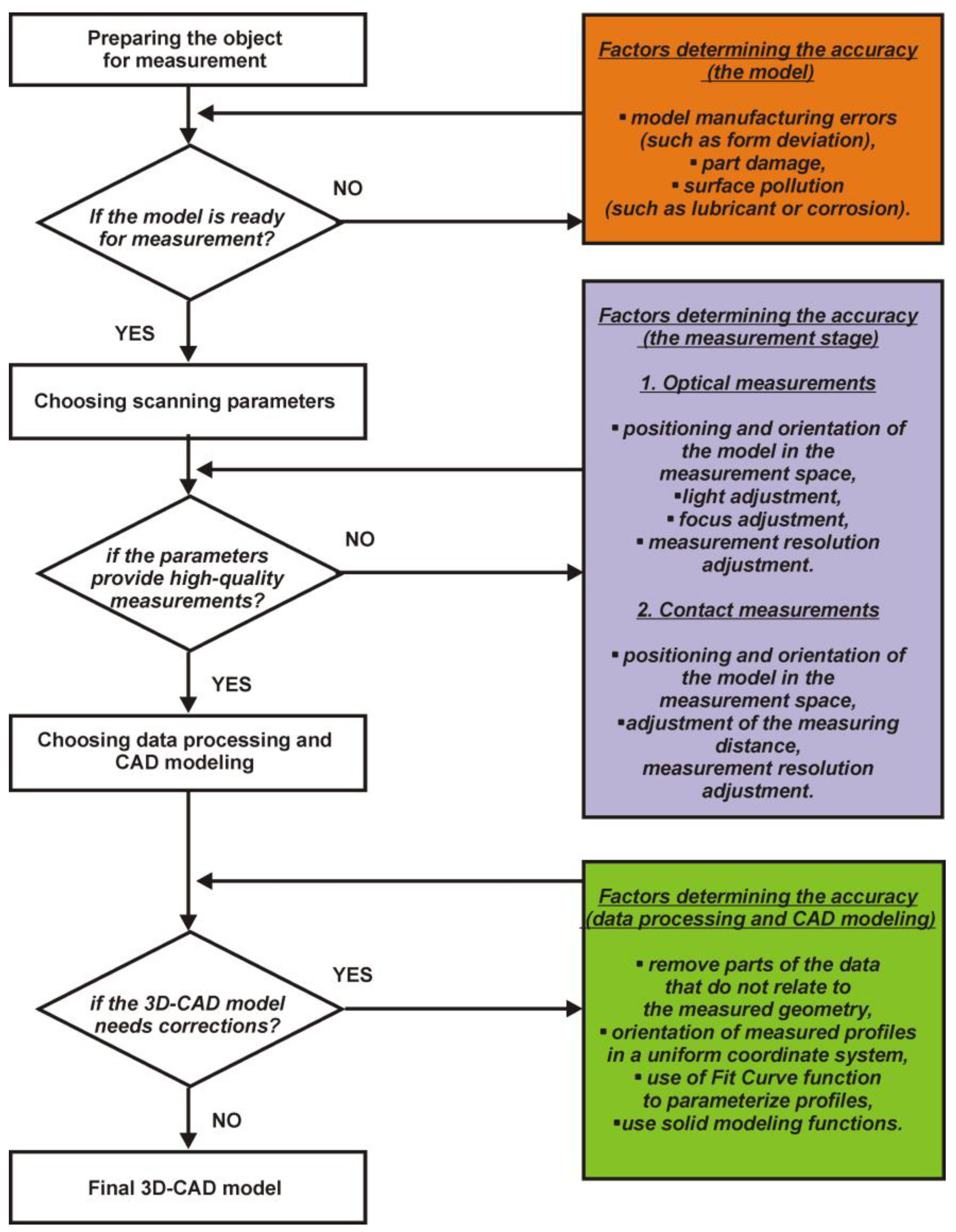Considering the research described in Figure 18, the factors influencing accuracy at the stages of geometric measurement, measurement data processing, and, finally, the CAD modeling process were identified.

Two methods were used in the CAD modeling based on 3D point clouds: one simplified the modeling process by creating 2D profiles based on the 3D point cloud, and the other developed a 3D-CAD model by fitting traditional geometric figures (e.g., cylinder, flat surface) and freeform surfaces. Considering the data obtained with the laser scanner, an irregular form of a three-dimensional point cloud was observed. It was formed by manually merging the acquired data from different measurement directions. The maximum fitting error of the point cloud was 0.006 mm for the model used for clamping and positioning parts in the machining process and 0.01 mm for the connecting rod. The highest measurement resolution of the laser scanner, which was 0.01 mm, was used to minimize measurement errors. Despite this, an incomplete representation of the geometry of the models was obtained on selected sharp edges, which was combined with the limitations of the laser head itself.

Thus, most negative deviations were obtained from models scanned using this method. Most of them were within the ±0.05 mm deviation range. In the case of the model used for clamping and positioning parts for performing the machining process, the highest average values of the deviations of the fit of the line and circle for the parameterized profiles were below −0.1 mm. Thus, they did not exceed the deviation limits for the model’s manufacture. The dimensional and form tolerances of the model were within deviations of ±0.1 mm. The model was designed for the company’s domestic production needs. In the case of the connecting rod, the results of matching the flat surface and cylindrical surface to the three-dimensional point cloud were also below −0.1 mm in some places. The fitting deviations were much higher for some sections of the connecting rod, mainly due to the wear of the model’s surface in this area. The degree and tolerance method fitted the profile with a spline curve for a section of the connecting rod geometry. Based on the generation of a three-degree curve and an assumed tolerance of 0.01 mm, an average fitting error of 0.005 mm was obtained. Thus, the errors of the entire reconstruction process were mainly within the manufacturing tolerances of the connecting rod. Unfortunately, the errors created in the operation process significantly affected the increase in the values of negative deviations in the big end bore. In the case of the wrist pin diameter, the deviations were much smaller and, in most areas, did not exceed the values of manufacturing deviations [51,52]. The deviation of the hole axis spacing was −0.02 mm; the value obtained was within the range of manufacturing deviations, which is ±0.05 mm. 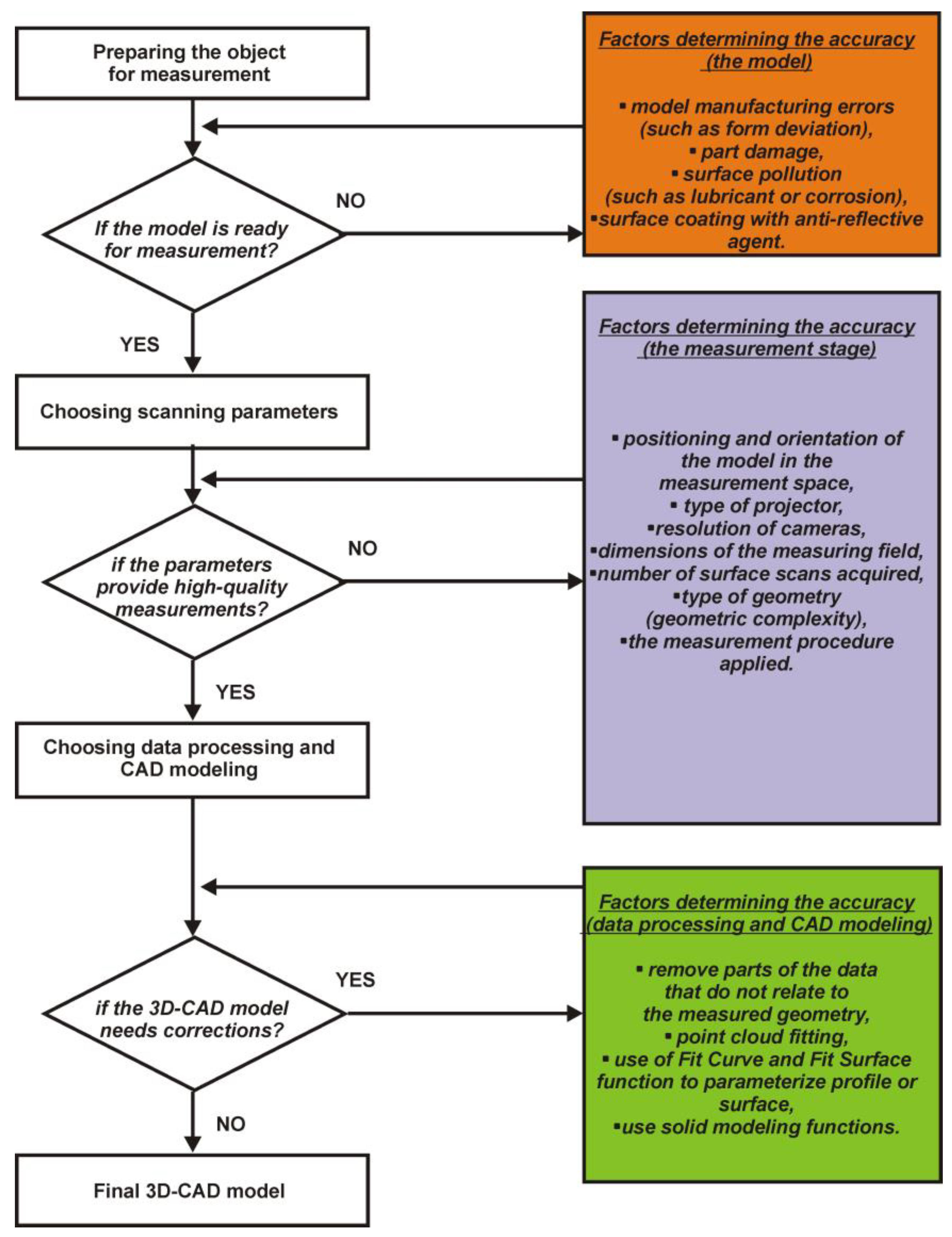Considering the research described in Figure 19, the factors influencing accuracy at the stages of geometric measurement, measurement data processing, and, finally, the CAD modeling process were identified.

In the case of data obtained from the structured light scanner, a more homogeneous point cloud was obtained. Thus, the error of fitting the point clouds for the turbine blade was 0.003 mm, and for the helical gear was 0.004 mm. This was due to the automation of the entire measurement process. The models of the turbine blade and helical gear were measured with a resolution of 0.01 mm to minimize the impact of measurement errors. The established resolution value was ten times smaller than the tolerances, which defined the accuracy of the model’s geometry [53,54,55]. For the turbine blade geometry, section curves were generated. Spline curves were created on the obtained points. Each profile consisted of four elements of this type, continuously connected. The profile’s leading edge, attack edge, and upper and lower parts were modeled separately. The Fit Spline command created approximated curves based on the imported points. Based on the generation of a three-degree curve and an assumed tolerance of 0.01 mm, an average fit error of 0.005 mm was obtained. The option to generate a section curve was also used for the helical gear. Similar settings to the Fit Spline option were applied to the turbine blade. However, higher average fit errors of about 0.1 mm were obtained based on the settings used. The highest modeling errors occurred within the spline area and the fragment of tooth geometry. These occurred because those areas were damaged. For the development of the side surface of the tooth, the Fit Surface option was used. The option chosen was Fit Freeform Surface. Based on the selected option, the accuracy of the modeling of the side surface of the tooth was obtained, which was within the range of maximum deviations of ±0.09 mm. Considering the research described in Figure 20, the factors influencing accuracy at the stages of geometric measurement, measurement data processing, and, finally, the CAD modeling process were identified.

In the case of models of anatomical structures, it is impossible to relate the results obtained to the accuracy of nominal models (since such do not exist). However, several conclusions can be made about the factors affecting the accuracy of the reconstruction process. Among the most significant are errors in the measurement process, which largely depend on the quality of the spatial resolution of the DICOM data [56,57]. 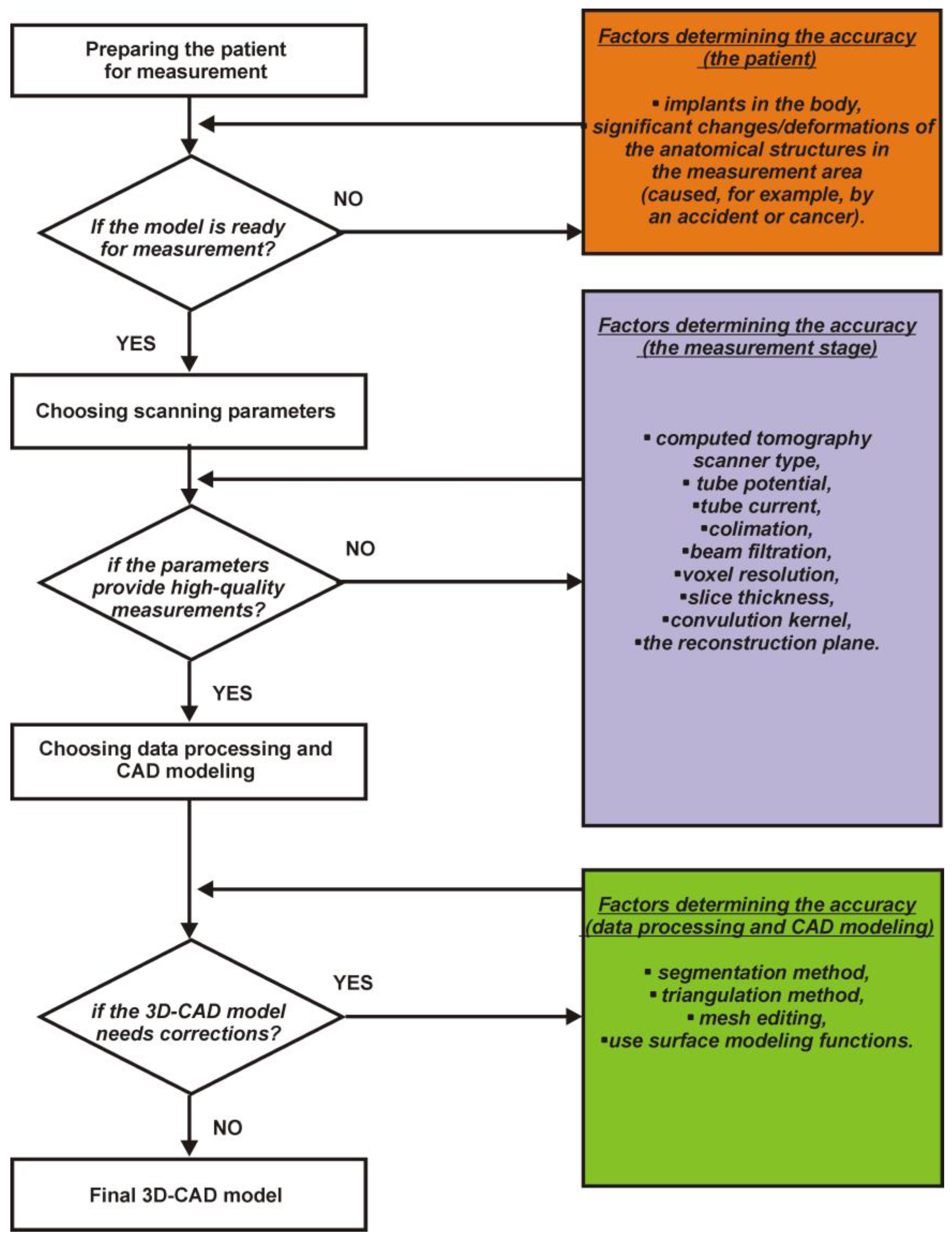In addition, the accuracy of the obtained geometry is also influenced by the segmentation method used [30,58]. Additionally, it is crucial to know the CAD modeling errors. For models of anatomical structures of the hip joint, the method used was to generate an automatic freeform surface based on curves previously projected onto the 3D-STL model. For non-standard geometries such as anatomical structures, no other 3D-CAD modeling method was possible. To fully parametrize the models, in the case of the femur model, 1060 edges were required to be generated, on which 530 surface patches were spanned. For the pelvic part, 1248 edges were generated, on which 624 surface patches were spanned. The generated parameters achieved CAD modeling accuracy of ±0.2 mm for the femur model and ±0.1 mm for the pelvic part. As with any modeling method, it is possible to develop 3D-CAD models more accurately. This is especially possible for the femur. However, covering the 3D-STL model with a larger number of surface patches significantly increases the 3D-CAD model generation time. Considering the research described in Figure 21, the factors influencing accuracy at the stages of geometric measurement, measurement data processing, and, finally, the CAD modeling process were identified.

5. Conclusions

Reverse engineering is becoming increasingly crucial in reconstructing the geometry of models for which we usually do not have technical documentation. The most significant problem concerning the reconstruction of geometry is related to the occurrence of errors that influence the accuracy of the development of the final 3D-CAD model. The lack of developed procedures and estimated errors at the stage of geometric reconstruction carries the risk that selected dimensions and, most importantly, functional parts of the reconstructed model may be outside the tolerance limits. Therefore, the procedures developed in the article, including the selected resolution of measurement systems, constitute CAD modeling methods to minimize reconstruction errors, allowing the development of copies of model geometries within the tolerance limits of their manufacture. The selection of the system and measurement parameters, the accuracy of fitting together the acquired measurement data, and the parameterization methods used have a major influence on the deviation values obtained. However, all co-authors confirm that it is necessary to test the adopted assumptions further to optimize the presented procedures and to test their functional properties on already manufactured models whose digital documentation was created in the reconstruction process.