Simulation of a Small Smart Greenhouse

Abstract

This paper investigates the design and implementation of a small greenhouse, based on an estimation of the required annual electrical loads, using robust energy modelling free software, namely OpenStudio. The greenhouse optimum materials, shape and orientation were estimated from this software, using weather file data and established environmental set points. Real-world electrical load estimations for the temperature, irrigation and lighting subsystems were consequently made, resulting in a good estimation of the required solar panel and battery combination. Sensors and actuators to physically establish the environmental set points were described, controlling with a microcontroller, while minimizing power losses. To maximize power throughput to the battery, a maximum power point tracking algorithm was described and modelled in Simulink, specifically for this system, using the microcontroller to implement a Perturb and Observe algorithm.

1. Introduction

Greenhouses are widely used to create suitable environmental conditions for the growth of plants. In the summer and winter, high and low temperatures can harm the plants. Too much water from the rain can suffocate plant roots. Errors in the irrigation frequency can induce irregularities and wither plant growth. This dependency on natural factors can be dangerous to certain fragile plants in traditional farming, taking into account the recent and future effects of global warming. At lower latitudes, in seasonally dry and tropical regions, crop productivity is projected to decrease for even small local temperature increases (1 to 2 °C), which would increase the risk of hunger. Specifically, in southern Europe, climate change is projected to worsen conditions (high temperatures and drought) in a region already vulnerable to climate variability, and reduce water availability, hydropower potential and summer tourism.

Furthermore, both climate change and population growth will likely cause reductions in arable land in Africa, South America, India and Europe.

Given these projections [1], there is a demand for fast and high-yield agriculture while occupying a relatively small area. This can be achieved by the use of greenhouses, in which environmental and climatic conditions can be adjusted according to the plants to be grown while the structure can provide protection from external factors.

Human error while maintaining climate control can affect the growth rate of the plants present in the greenhouse. For this reason, human intervention is minimized with the automatization of the internal climate control, minimizing water consumption as a consequence.

The strict automatic climate control, physical protection and better yield rates provided by greenhouses can be the solution to the presented problems. To further increase the robustness of the system and decrease the ecological footprint, a photovoltaic system can be added to the system.

In recent decades, several studies have been carried out regarding the implementation of new forms of greenhouse management. The most recent work [2] is a comprehensive framework for understanding the actual greenhouse development in Qatar to support its transition to sustainable precision agriculture

Over the years, greenhouse monitoring has become essential for efficient sustainability agriculture growth. For this purpose, remote monitoring becomes crucial to have agriculture with a minimum of waste. Reference [3] summarizes the smart greenhouse IoT-based application, highlighting the benefits and opportunities of this technology in the agricultural environment.

Renewable resources are used to supply the sensors that motorize the greenhouse. For example, in [4] the authors review the literature regarding the applications of selective shading systems with crops, highlighting the use of photovoltaic panels.

In this paper the main goal is the design and implementation of a small smart greenhouse to minimize human labour and ecological impact by automatic climate control of the greenhouse in a way that promotes an ecological and self-sustainable lifestyle. The first steps in the design of the greenhouse and the underlying systems will be discussed, before the respective physical implementation. This greenhouse will be mainly oriented to use in Portugal, so some design decisions will be decided based on that. The following main steps describe what will be designed/chosen:

• Shape and materials of the greenhouse.
• Annual electrical load profiles
• Battery and PV array estimation
• Sensors and actuators
• Solar charging through maximum power point tracking.

This paper is organised into four parts. The first part is dedicated to the greenhouse design, with various scenarios regarding different types of materials, orientation and greenhouse shape. This is done with the help of building energy software, which integrates precise thermal models with the calculation of temperature and humidity based on weather files, set geometry and construction issues. The second part describes each subsystem (temperature, lighting and water irrigation) succinctly, through the exhaustive description of the sensors and actuators required. The power supplying analogue/digital control is explained for each instance while trying for optimal min/max efficiency, measurement accuracy and costs. Lastly, this all comes together with a model description and implementation in Simulink of the solar charging through maximum power point tracking, using the Perturb and Observe algorithm.

In the third part conclusions are drawn and in the fourth, future work is considered.

2. Energy Modelling

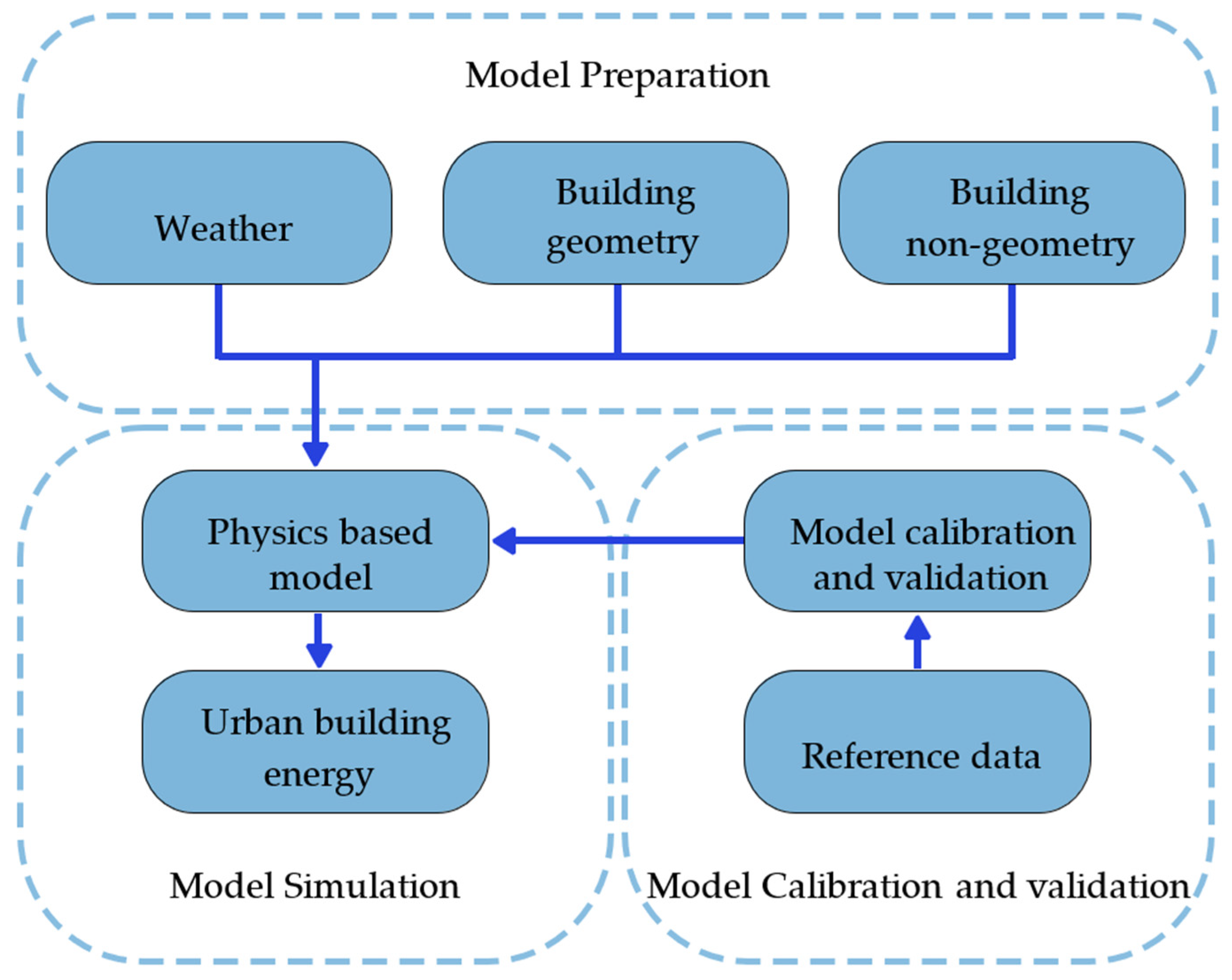
To help decide on the parameters that need to be taken into account so that crops get comfortable levels of temperature inside the greenhouse, energy simulation software is often used by designers. This type of software is usually capable of doing an entire year’s analysis of the indoor environment and energy use, based on the geometry, weather data, materials, loads schedules and so on [1]. Thus, it is possible to reduce energy and material costs while validating the internal environment with accuracy across the four seasons for a certain crop. In Figure 1, the essential steps are visualized as a flowchart of the inner workings and user-defined parameters of a general energy modelling software with a physics-based bottom-up model.

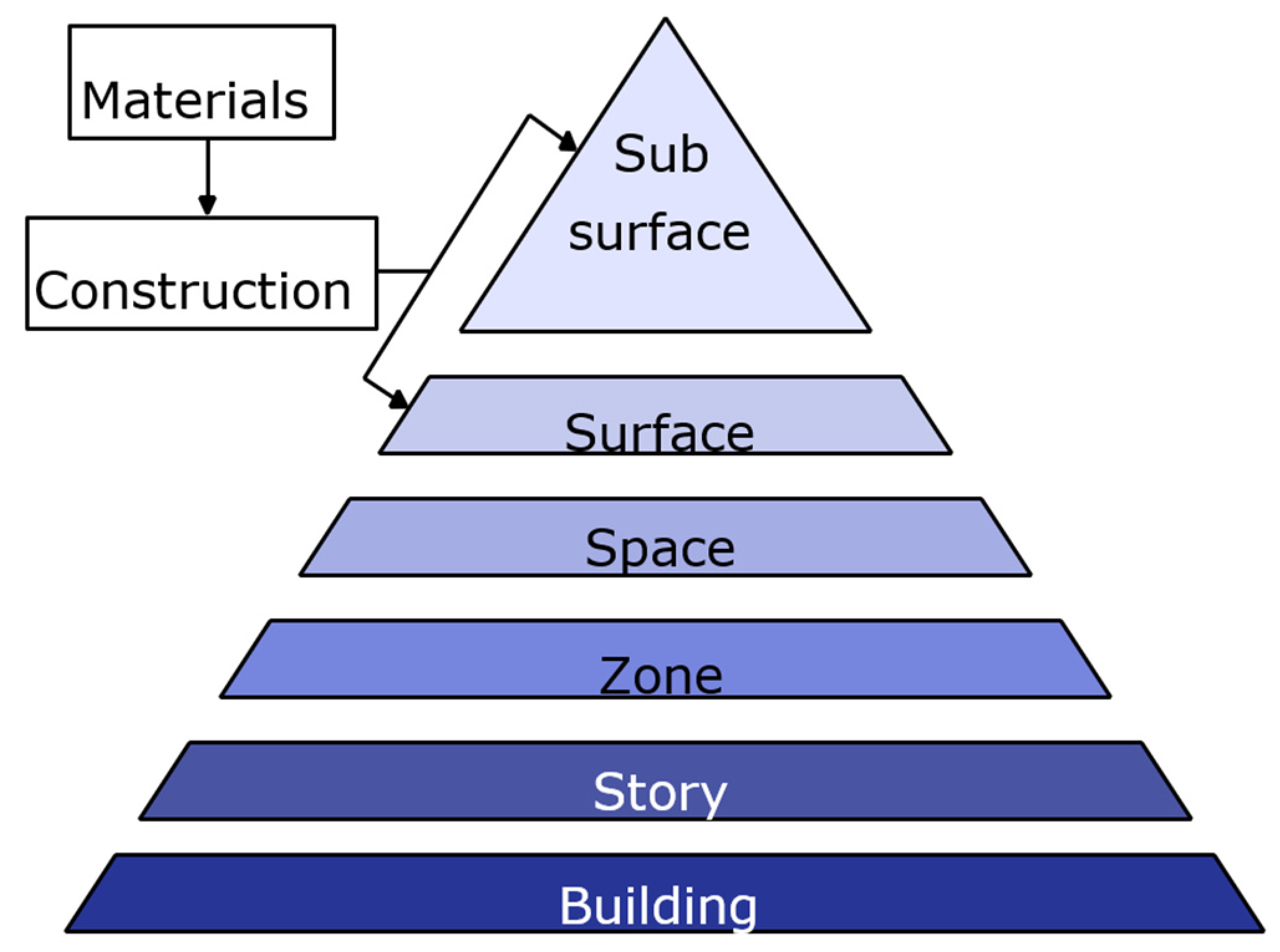
EnergyPlus was the chosen software because it has a more energy modelling refined temporal resolution (sub-hourly) [2], which is a major feature for scheduling the loads in the HVAC systems for the greenhouse. OpenStudio was used as the GUI for this engine. To better understand the building envelope geometry of an OpenStudio model, the various hierarchy-based abstractions of OpenStudio and EnergyPlus are presented in Figure 2.

For an objective judgement of the temperatures for optimum tomato growth, a temperature interval for a tomato crop must is defined.

Table 1. Optimum temperatures for tomato growth [3].

Time	Optimum Temperatures [°C]
Daytime	18–25
Night-time	10–20

shows such an interval.

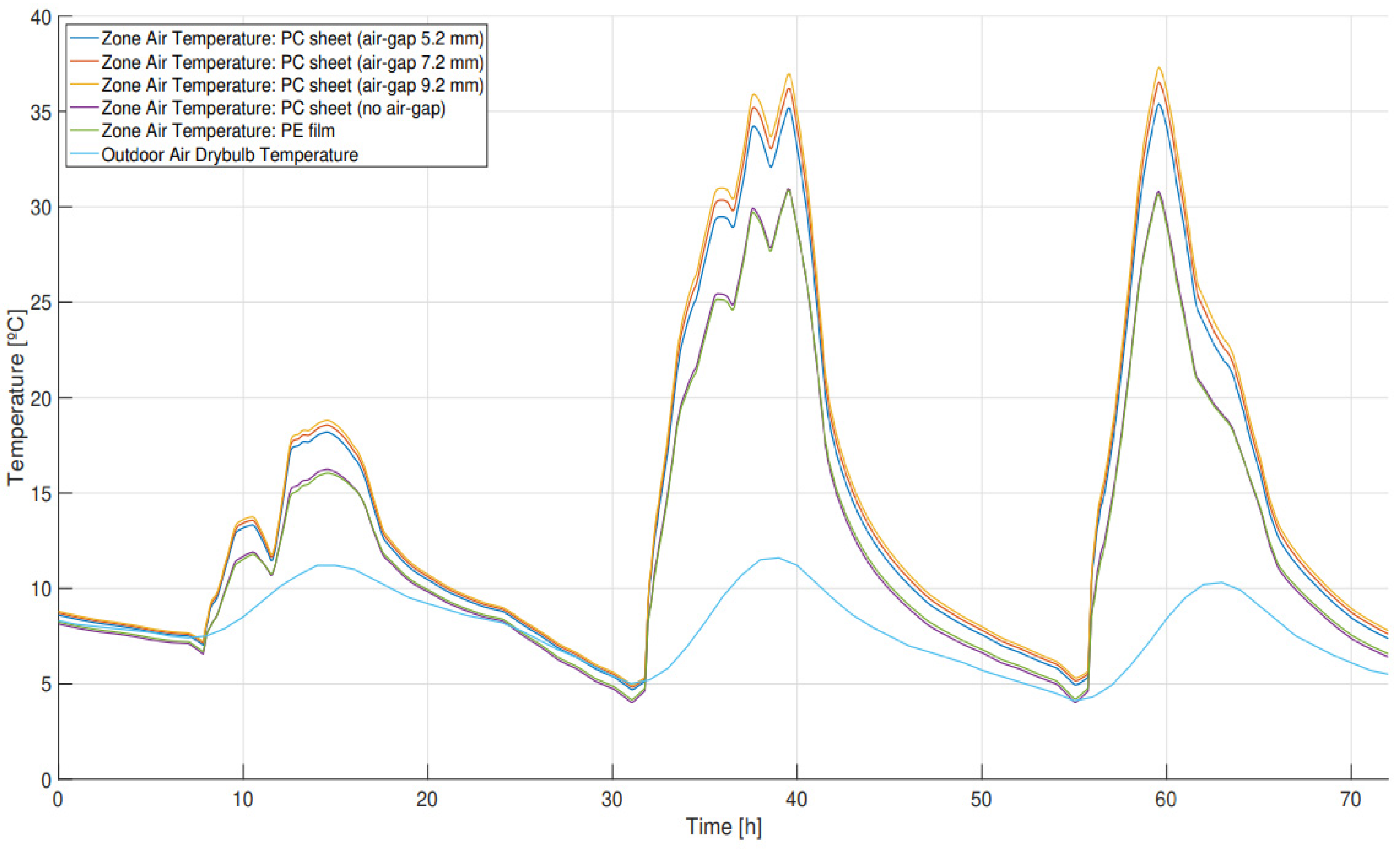
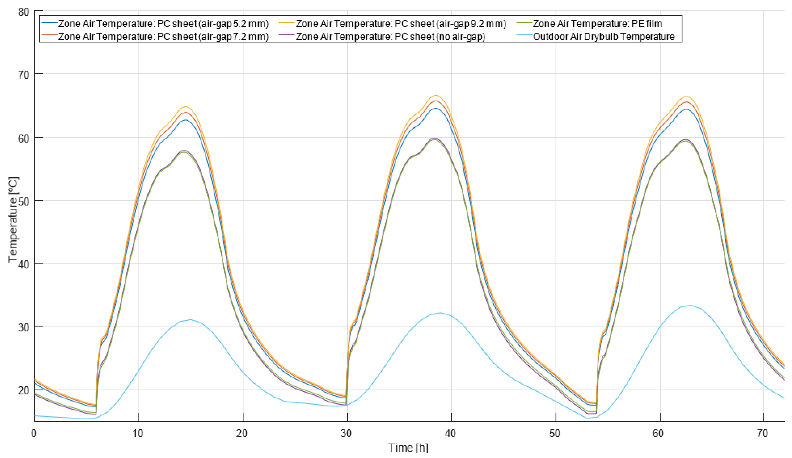
As expected, comparing these intervals with the temperature inside the greenhouse, it is safe to say that both a heating and cooling load is required for the crops to survive. Figure 3 shows that the temperature reaches a few degrees below 10 °C (reaching below 5 °C as the minimum) for the whole night. Figure 4 shows that the temperature reaches 2 to 3 times the defined maximum optimum temperature (reaching as high as 65 °C). For a better evaluation during the whole year, the heating and cooling energy demands must be defined, considering the intervals that were established for this crop. The schedules were set and the Ideal Air Loads were turned on for the single Thermal Zone in this model. 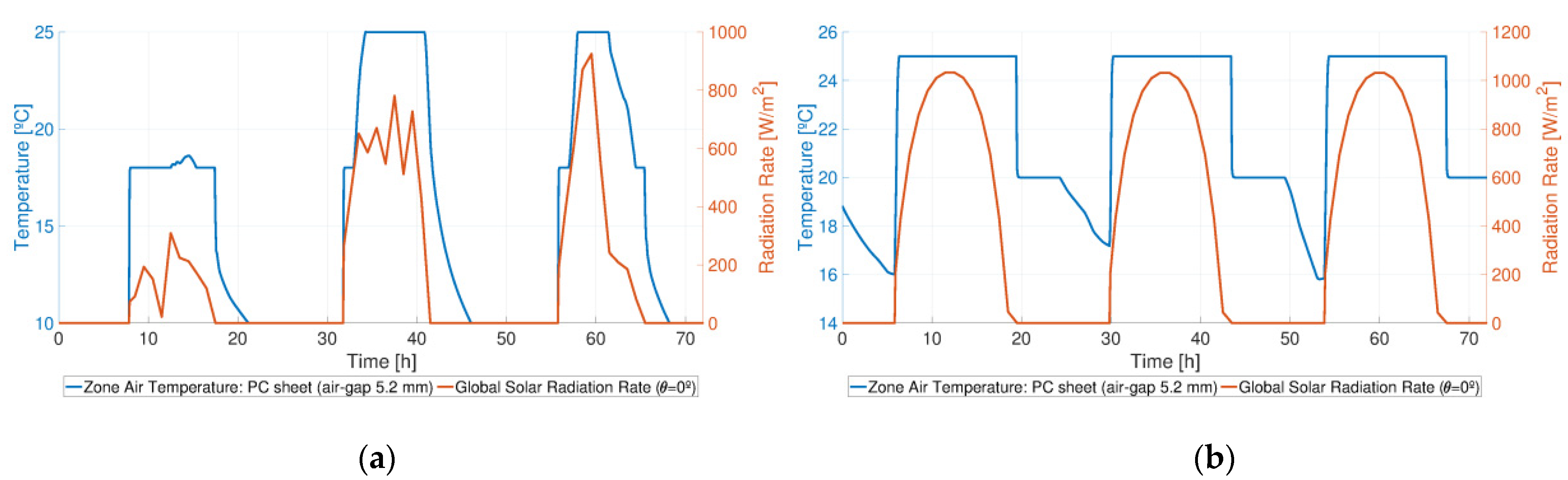Figure 5 shows the temperature inside the greenhouse using one of the glazing materials (PC sheet (air-gap 5.2 mm)) and with the GHI. 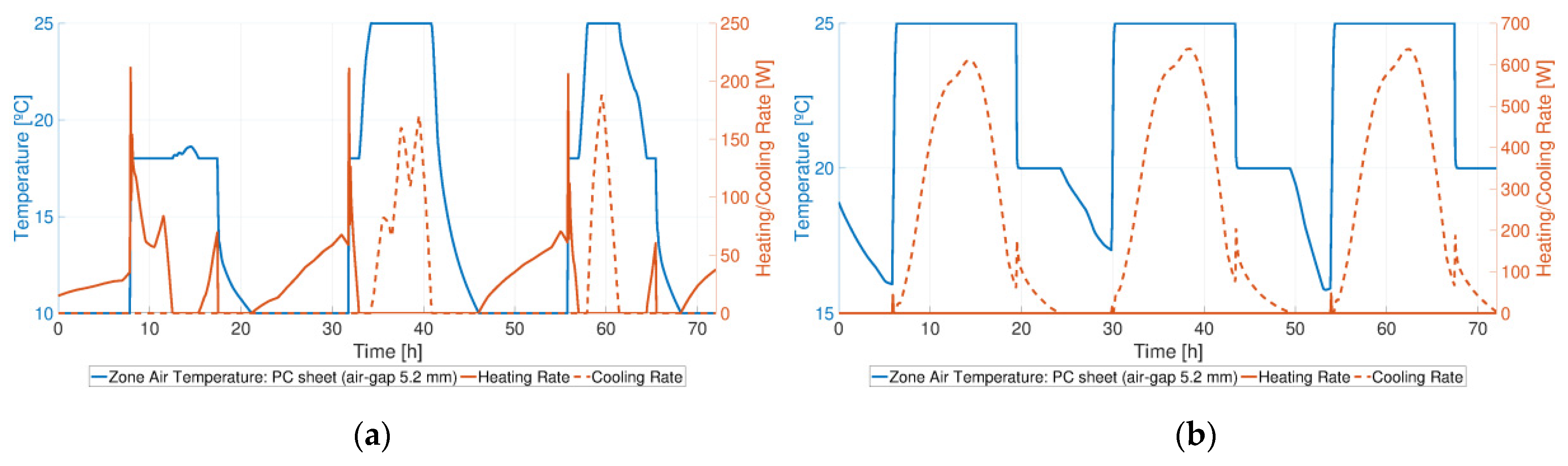Figure 6 shows the same temperature but is accompanied by the ideal heating and cooling rates.

As can be observed, the temperature for these extreme days is now “chopped”, to maintain the temperatures intervals that were previously set. The ideal heating and cooling demands automatically increase and decrease in value based on need. Having the heating and cooling rates, the total annual energy required (E_Htg,Clg) is obtained by the sum of every heating/cooling rate required (P_Htg,Clg) for every timestep of the yearly simulation. This relation is expressed in Equation (1).

$${\sum }_{n=1}^{n_{max}}{P}_{Htg,Cl{g}_n}=E_{Htg,Cl{g}_n}$$

(1)

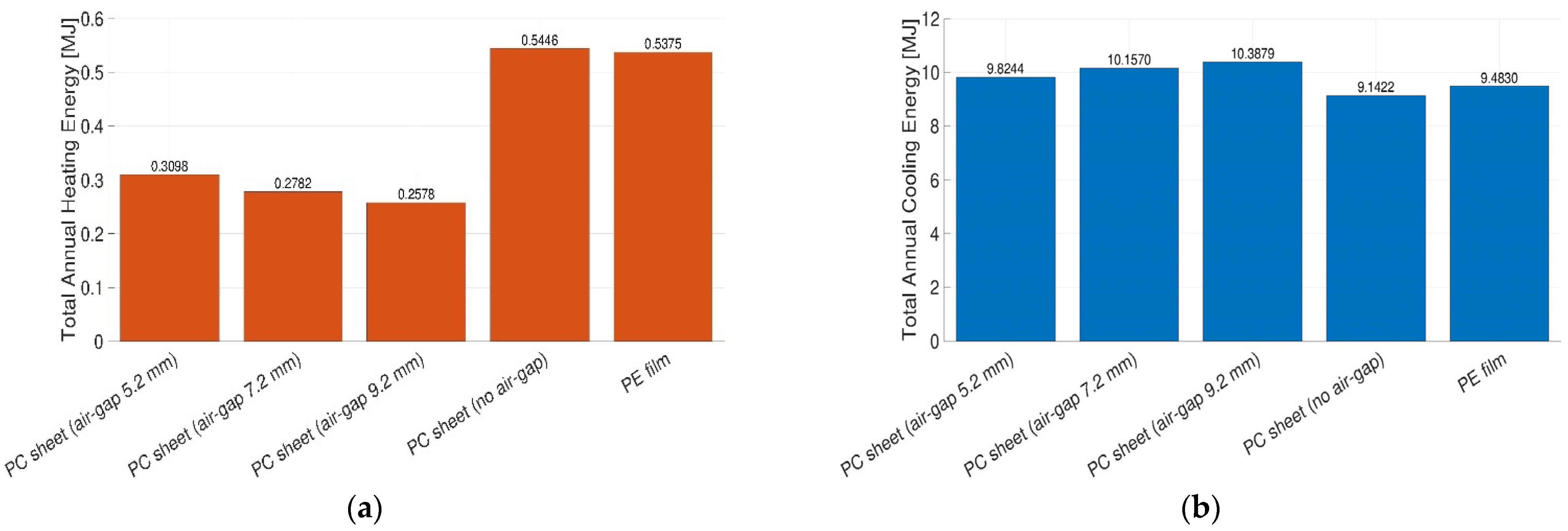
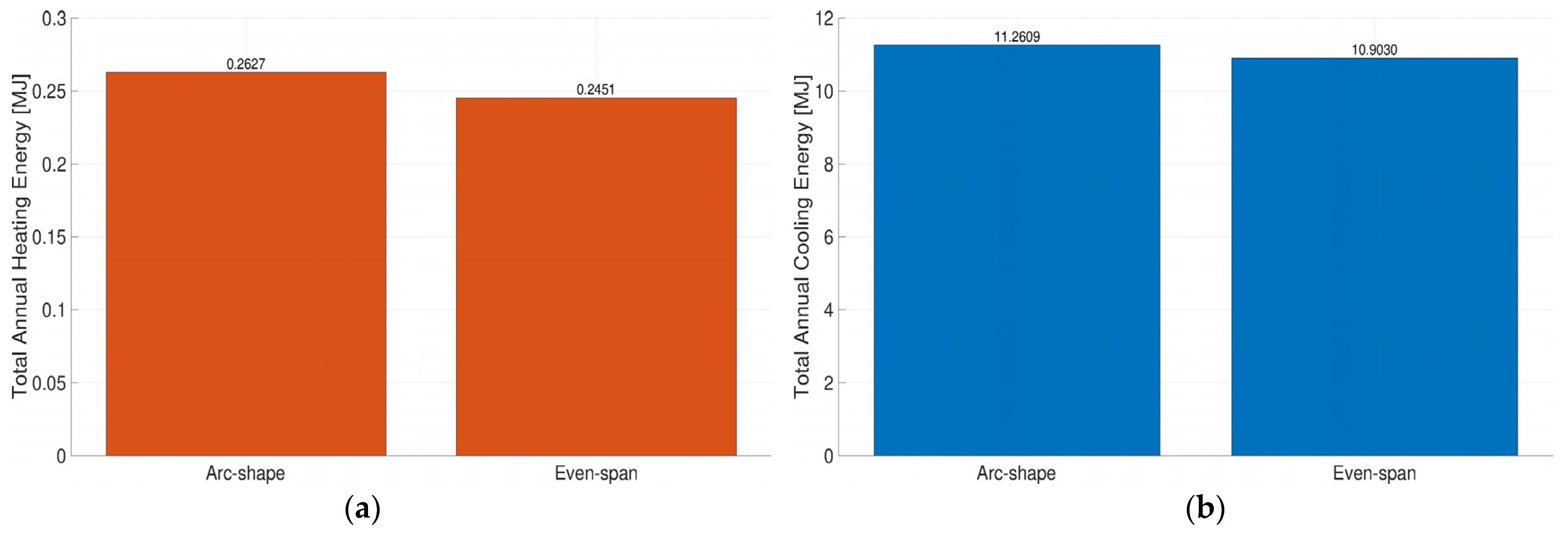
with n being the current timestep and n_max the total number of timesteps of the simulation. Figure 7, Figure 8 and Figure 9 show the ideal annual energies required for both heating and cooling, comparing the different scenarios established in

Table 2. Scenarios for the geometry and non-geometry parameters of the greenhouse.

Parameters	Scenarios
Glazing constructions	PC sheet (3 mm no air-gap) PC sheet (0.4 mm air-gap twin-wall) PE film (0.2 mm no air-gap)
Orientation	North-South East-West
Shape	Even-span Arc-shape Quonset

.

In conclusion, the following scenarios were chosen:

• Glazing Material: PC sheet (air-gap 9.2 mm);
• Orientation: East-West;
• Shape: Even-Span.

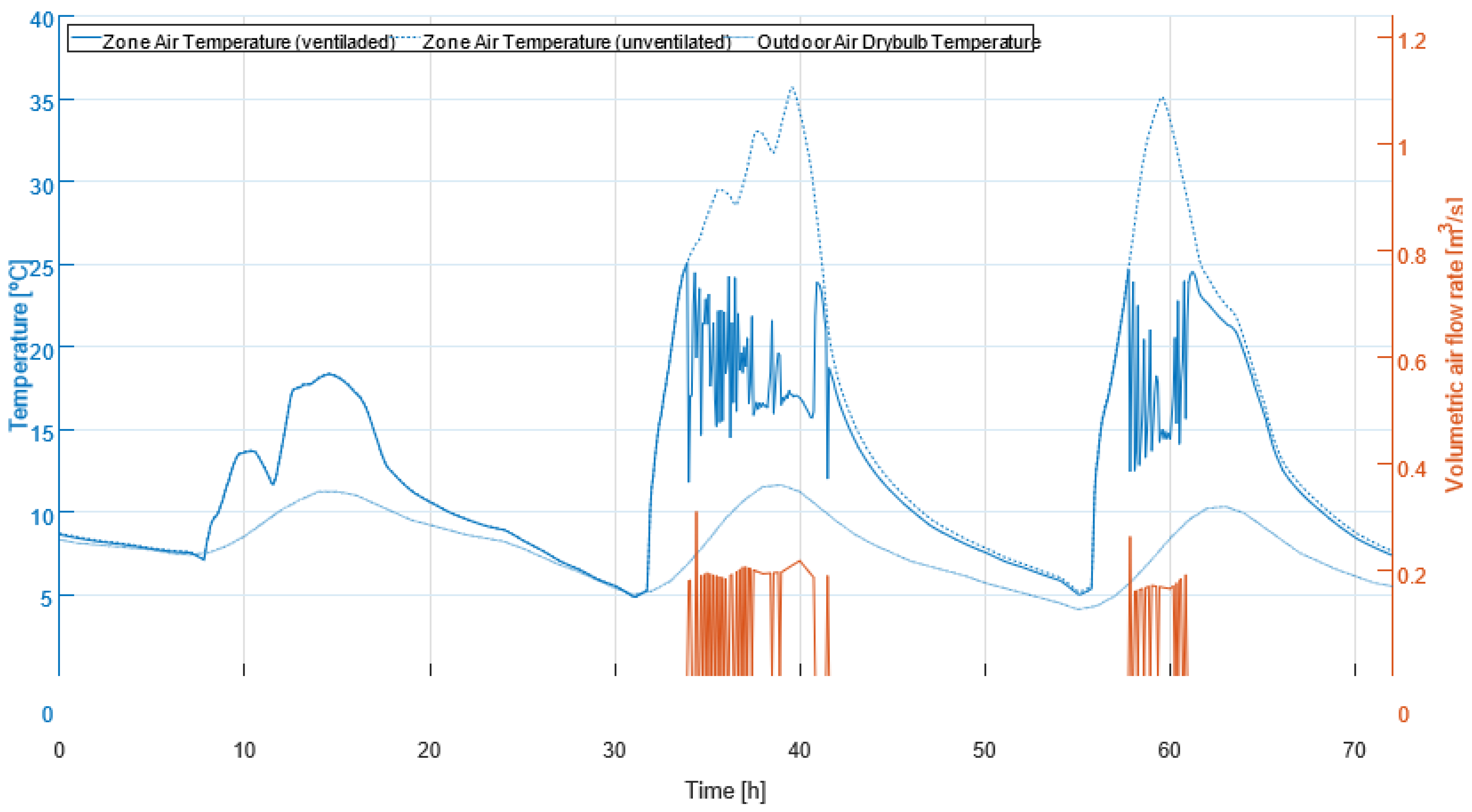
Ideal Air Loads were used to compare the performance of the annual heating and cooling demands of the different proposed scenarios. These loads will be substituted by real world electric loads. In OpenStudio, natural ventilation is accomplished by a Zone Equipment in a Thermal Zone called Wind and Stack with Open Area, in which the ventilation air flow rate is a function of wind speed and thermal stack effect, along with the area of the opening being modelled. The ventilation rate driven by wind (Q_W [m³/s]) is given by Equation (2)

Q_W = C_W · A_opening · F_schedule · v

(2)

with C_W being the opening effectiveness, A_opening the opening area [m²], F_schedule the open area fraction and v the local wind speed [m/s]. If the C_W input field is set to “AutoCalculate”, the opening effectiveness is calculated for each simulation time step based on the angle between the actual wind direction and the Effective Angle [deg] (a user-defined input) using Equation (3).

$$C_W=0.55-\frac{\left|EffectiveAngle-WindDirection\right|}{180}0.25$$

(3)

The ventilation rate driven by the stack effect (Q_S [m³/s]) is given by Equation (4)

$$Q_s=C_D{A}_{op}{F}_{sche}\sqrt{2g\mathsf{\Delta }{H}_{NPL}\frac{\left|T_{zon}-T_{odb}\right|}{T_{zon}}}$$

(4)

with C_D being the discharge coefficient for opening, ∆H_NPL the height from lower opening to the NPL [m], T_zone the Zone air dry bulb temperature [K], T_odb the local outdoor air dry-bulb temperature [K]. The total natural ventilation rate for this model (Q_W,S) is calculated as the quadrature sum of the wind and stack components, given by Equation (5).

$$Q_{w,s}=\sqrt{Q_s^2+Q_w^2}$$

(5)

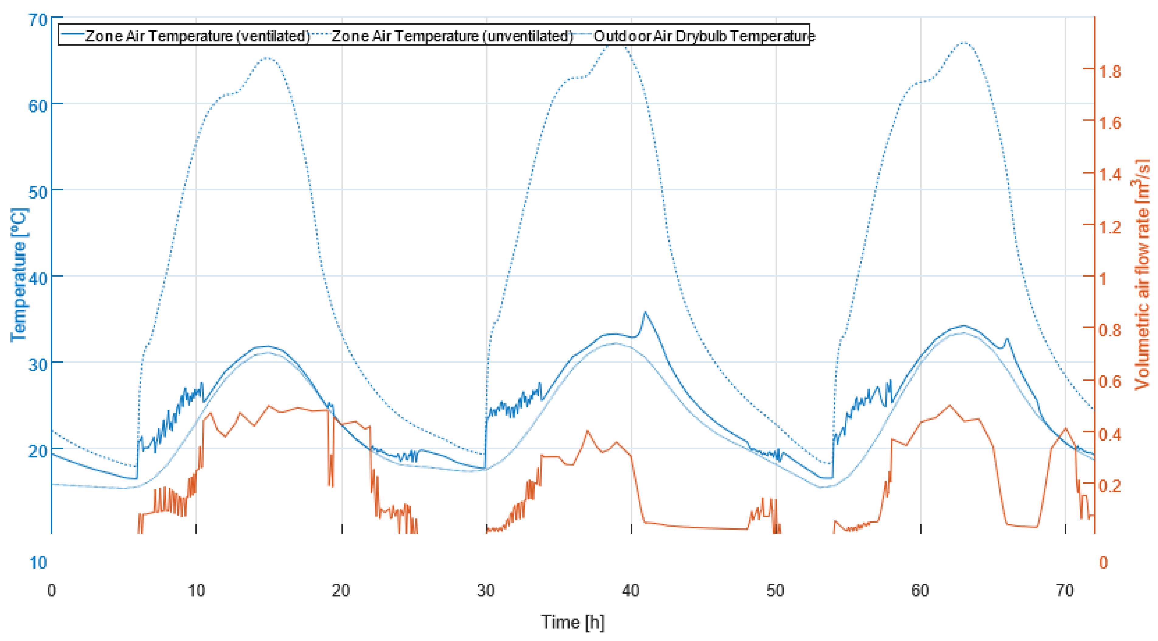
Figure 10 and Figure 11 show the simulation with ventilation results for the usual winter and summer days.

For lower latitudes and during the summer season, the wind and stack effect are not enough to protect the crops from the effect of solar radiation. Reduction of light can be obtained by shading of the greenhouse cover or application of shade screens [4]. The objective is to reflect as much sunlight as possible, and so metallic surfaces are often used as shades. A typical screen material is made of 4 mm wide aluminum and polyester strips held together with a polyester filament yarn [5]. OpenStudio has a type of material called Shade Window, which can be applied to certain sub-surfaces in the model. 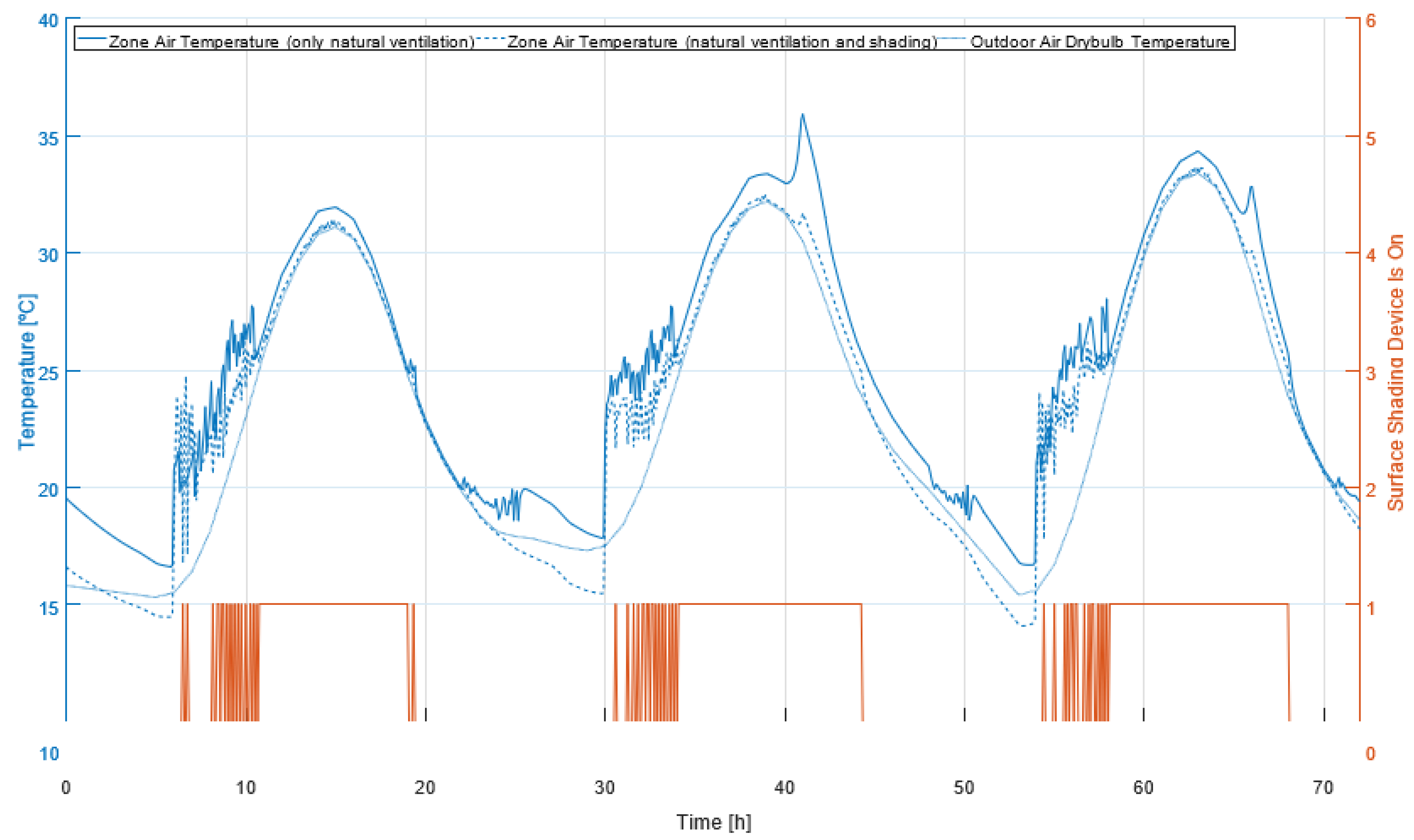Figure 12 shows the simulation with shading results for the usual summer days.

This figure shows that when there are relatively low wind speeds with high outdoor air temperatures (afternoon of 14 August), a shading device can reduce the inside temperature of the greenhouse. The temperatures during the coldest days would often reach below 10 °C, the minimum inside temperature set for the greenhouse. There are multiple ways to heat a greenhouse, but with electrical energy available (from the solar panel), the easiest way is to directly convert this electrical energy into thermal energy with 100% efficiency, by virtue of the Joule’s Effect, described by Equation (6)

$$P_h=IV=I^{2}R=\frac{V^2}{R}$$

(6)

With R being the resistance of the conductor which is dissipating the heat. To accelerate this heat dispersion, a fan is often placed close to this conductor, such that the sensible heat rate (P_h) is speeded up by the increase of the air flow rate (V˙), described by Equation (7)

P_h = c_pρV˙∆T

(7)

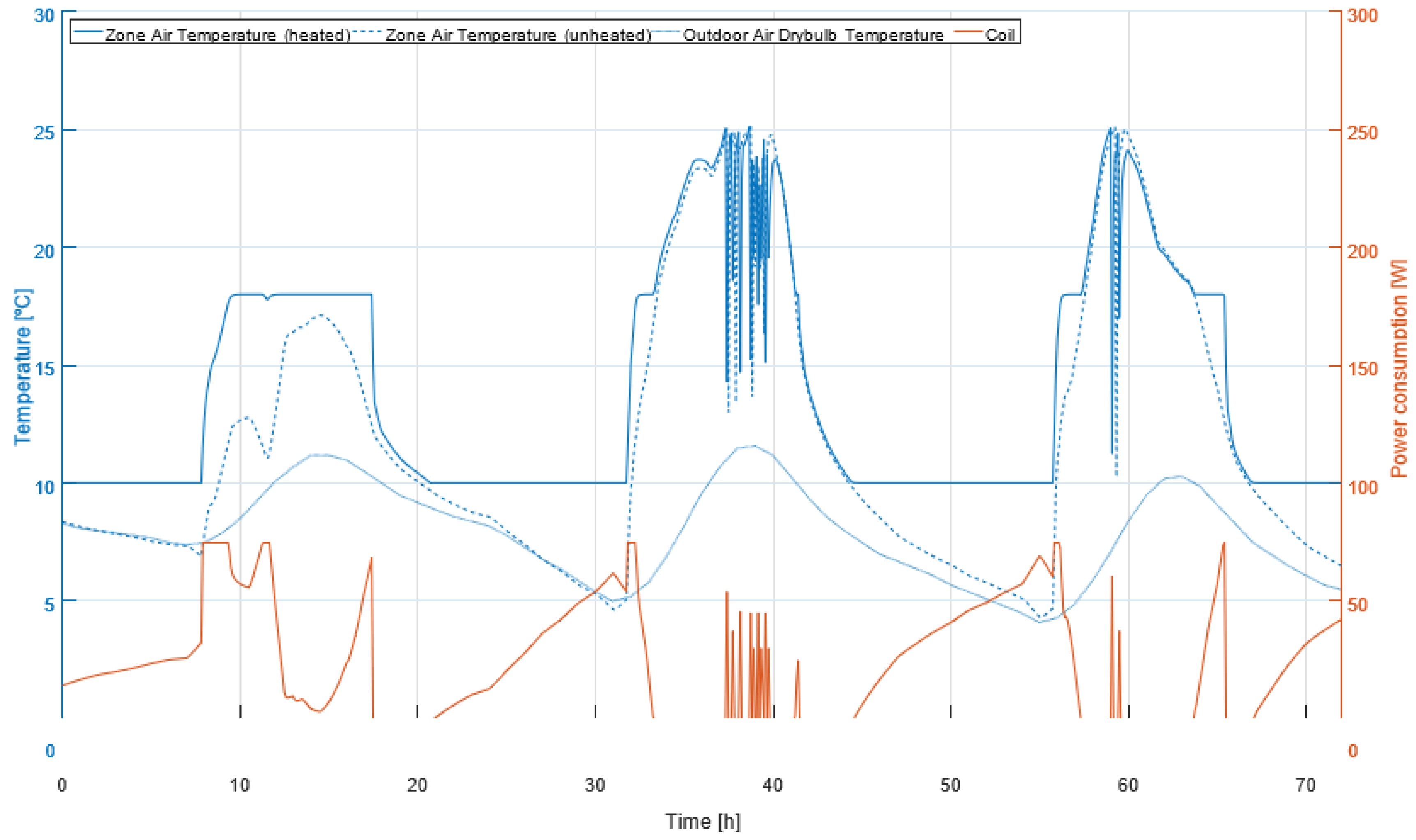
This 2 component system is applied in OpenStudio by using a Unit Heater, composed by a Constant Volume Fan and an Electric Air Heating Coil, which can be applied to a Thermal Zone. Figure 13 shows the results with this system.

In OpenStudio, to measure the amount of light in the growing area, Radiance is used, which is a ray-tracing software designed for the analysis and visualization of lighting in design. Using lux to measure the light intensity of horticulture lighting systems will give varying measurements depending on the spectrum of the light source. This is because photosynthesis is a quantum process and the chemical reactions of photosynthesis are more dependent on the number of photons than the energy contained in the photons. Therefore, plant biologists often quantify PAR using the number of photons in the 400–700 nm range received by a surface for a specified amount of time, or the PFFD. Values of PPFD are normally expressed using units of µmol/m²/s, given by Equation (8).

$$PPFD=8.35\times {10}^{-9}{\int }_{400}^{700}{I}_{\lambda }\lambda d\lambda$$

(8)

Numerical computations from photometric units to PPFD are usually done through conversion tables, using a multiplication factor (α) based on a well known spectrum (like sunlight), expressed by Equation (9).

PPFD = αI

(9)

In relation to plant growth, it is better to characterise the light availability for plants by means of the DLI, which is the daily flux of photons per ground area mol/m²/d, given by Equation (10) (86,400 refers to the number of seconds in a day).

$$DLI={10}^6{\int }_0^{86,400}PPFDdt$$

(10)

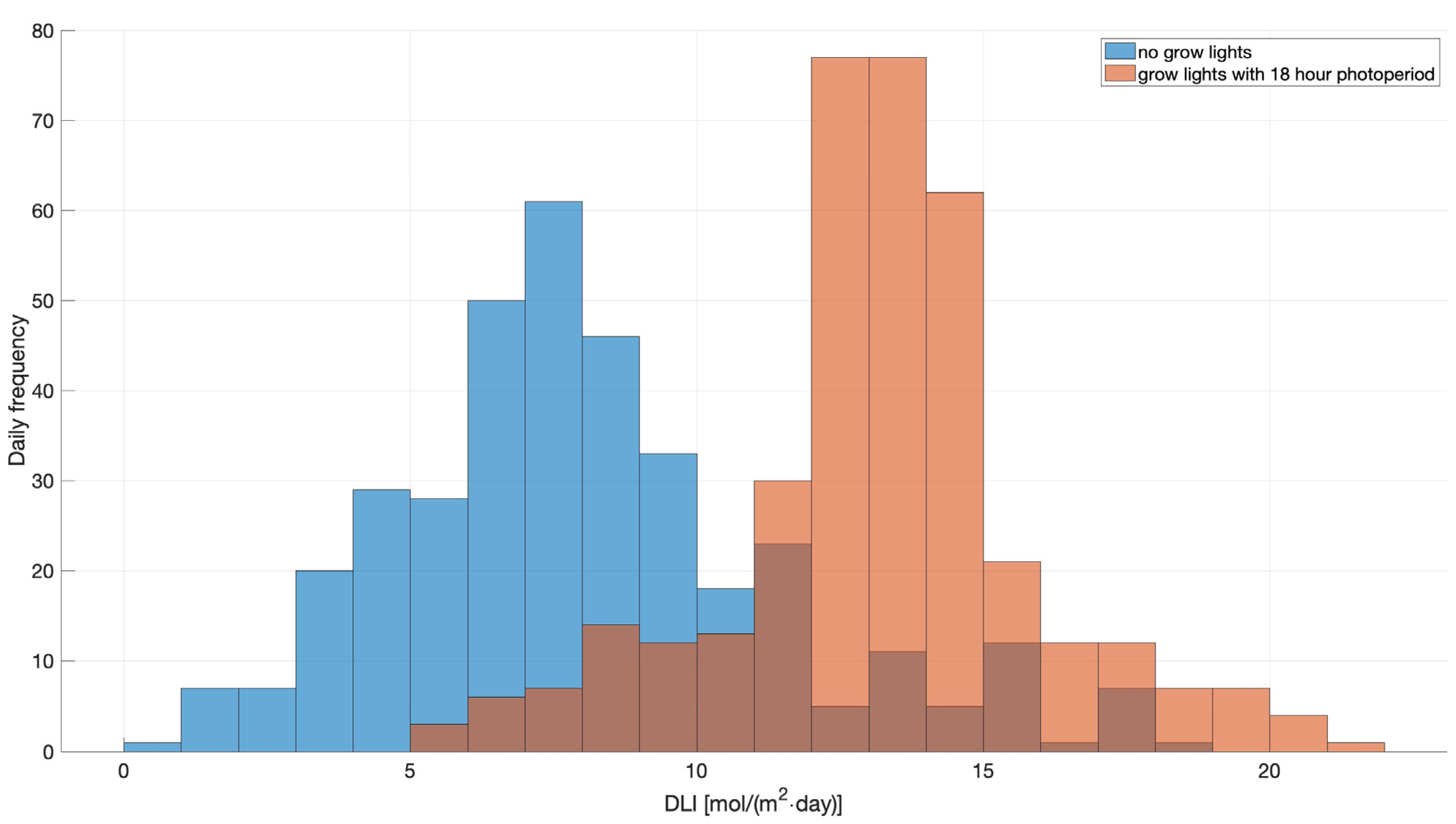
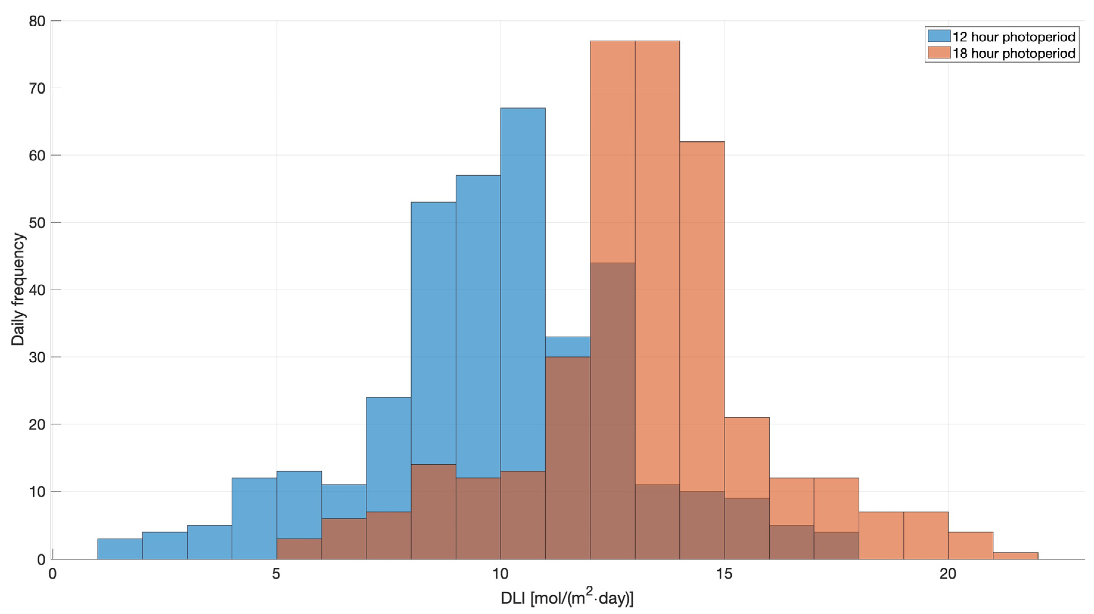
With the previous equations, converting the rated luminous flux to DLI for a specific photoperiod for every day of the year is possible. The ultimate goal is to have an estimation of the energy consumption of the light load, so a light schedule is required for OpenStudio, based on a comparison of the current calculated DLI and photoperiod to a target DLI and photoperiod for a given day, respectively. Figure 14 and Figure 15 show the result of this algorithm.

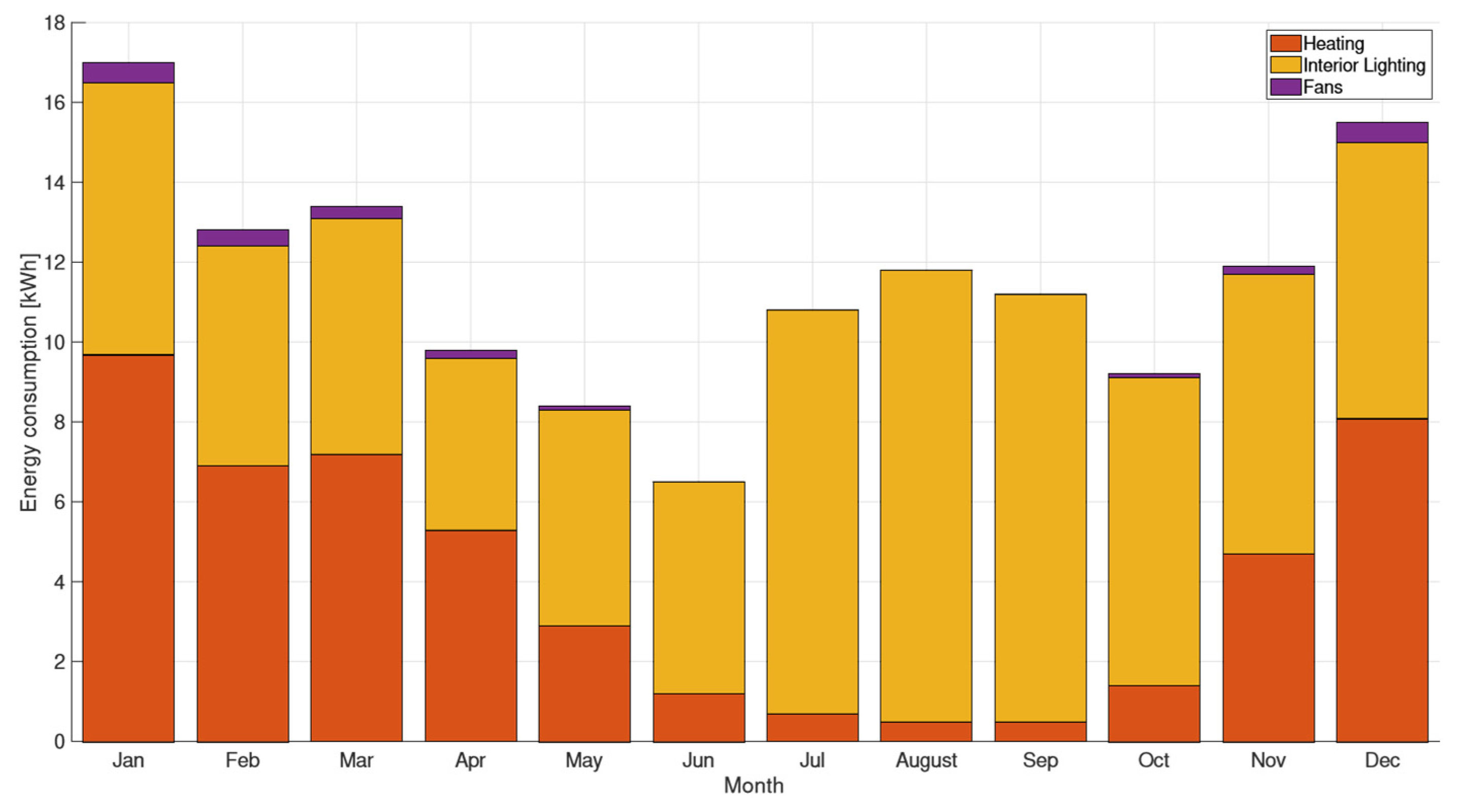
Figure 16 shows an overview of the monthly load contribution.

With all the required loads defined, it is now possible to define the battery and photovoltaic panel combination. OpenStudio has an energy generation feature with photovoltaics, such that for each simulation step the energy generated by the panel is calculated based on the irradiance present in the shading surface with the photovoltaic array. This photovoltaic array is modelled by the calculation of the power generated by this array (P) based on user-defined data and solar irradiance (G_T) from the weather file and the geometric model for solar radiation [6]

P = A_surf · f_activ · G_T · η_cell · η_invert

(11)

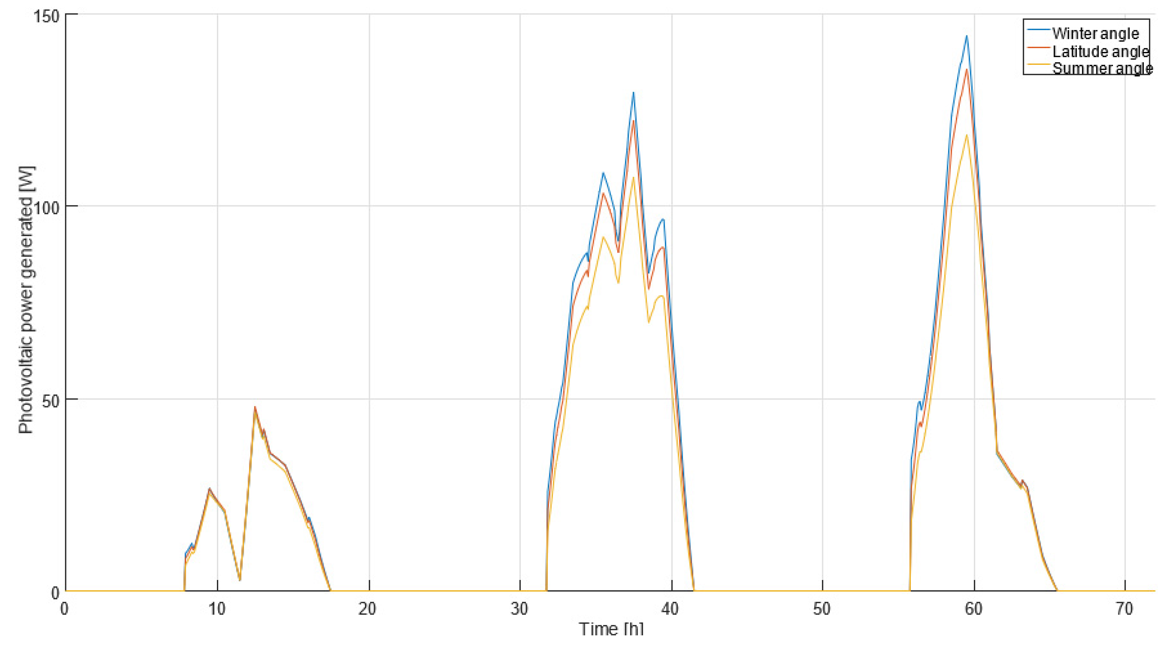
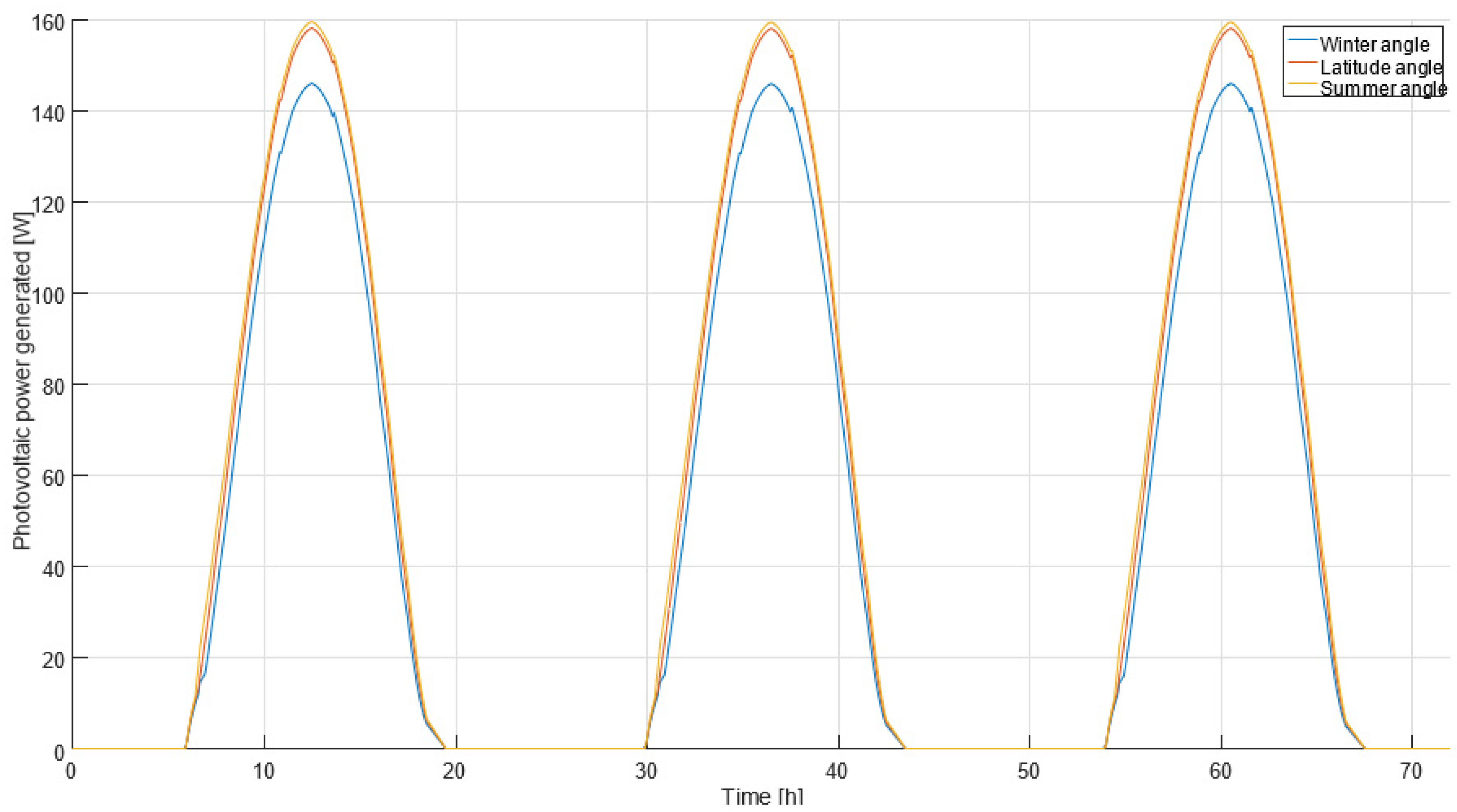
with A_surf being the surface area of the array, f_activ the fraction of active photovoltaic area, η_cell the efficiency of the solar cells and η_invert the DC to AC efficiency of a hypothetical inverter. For the surface area, a baseline peak power (for STC) was considered, so that this power requirement is higher than the sum of all the considered loads combined. This way, it is guaranteed that the charge of the battery at the end of every year is not lower than the previous year. This peak power is around 130 W, and 150 W photovoltaic panels are common in the market, so the area for this panel was considered. The photovoltaic panel tilt is also considered, as different values for the angles will give different average power outputs during the different seasons (Figure 17). Three cases were considered for this parameter: a “Winter angle”, a “Latitude angle” and a “Summer angle”. To compare the effectiveness of each angle, the power generated is compared for the usual winter and summer days. Figure 18 and Figure 19 show the result of the simulation.

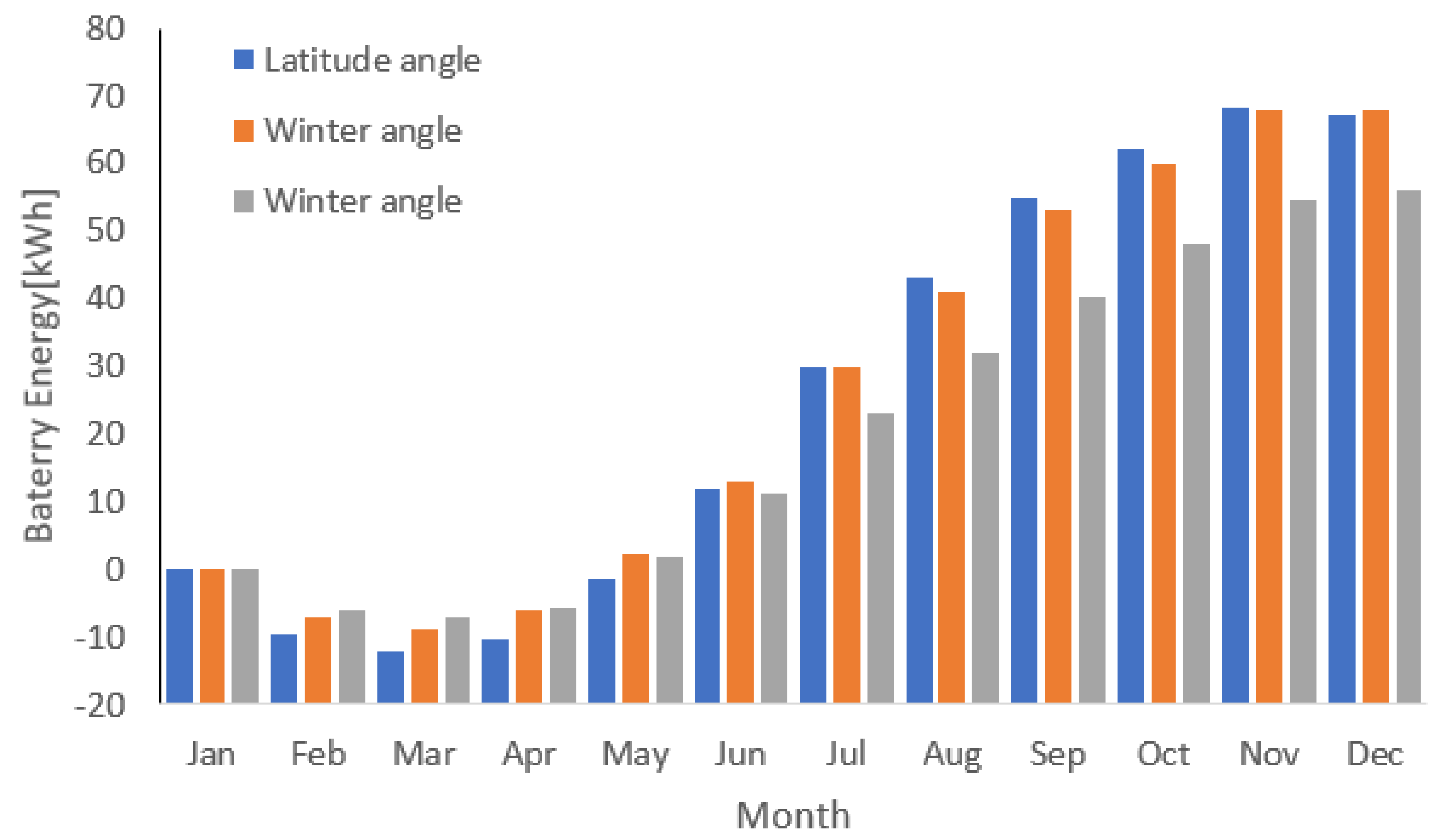
The obvious decision would be to choose the angle that generates the most energy, which would be the latitude angle. This is an oversight for this situation, as the energy available during the winter is much lower, while the load requirement is higher, when comparing to the rest of the year (illustrated by Figure 16). This problem is better explained by modelling the power flow of the PV panel-battery-loads system, while considering the battery as an “energy buffer”, showing the amount of energy present in the battery for every iteration for the entire year. This energy will be the sum of the energy coming from the PV panel (E_PV ) and the energy used by the loads (${\sum }_{m=1}^{m_{max}}{E}_{load}$). Equation (12) shows the relation described.

$$E_{ba{t}_n}=E_{ba{t}_{n-1}}+E_{P{V}_n}{\eta }_{bat}-\left(1-{\eta }_{bat}+1\right){\sum }_{m=1}^{m_{max}}{E}_{loa{d}_n}$$

(12)

with n being the current time step, n − 1 the previous time step, and η_bat the battery efficiency. For now, the battery technology is assumed to be lead acid and its efficiency to be 80%. This efficiency is formally defined as the “Energy Efficiency”, which is a measure for the amount of energy that can be taken from the battery compared to the amount of energy that was charged into the battery beforehand [7].

With the 3 different PV generation values, using Equation (12) results in 3 different battery energy values, shown in Figure 17. Because physically energy cannot be a negative value, this battery acts as a “virtual battery”.

3. System Monitoring and Electrical Description

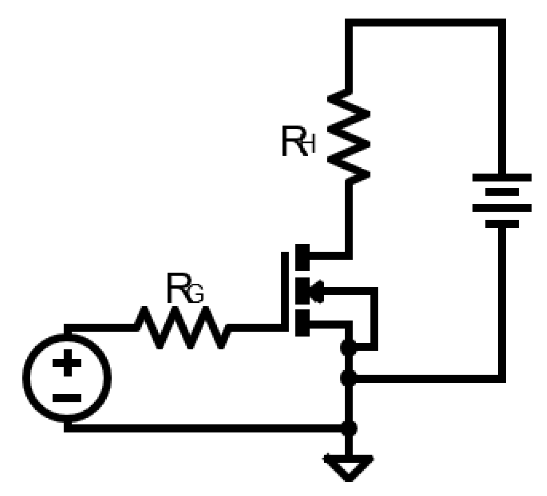
In the energy modelling software, the model would automatically control the input power value based on the required power output to maintain the greenhouse temperature at the established set temperature. A PWM controlled resistor is used. The power switching element can be achieved with an n-channel MOSFET. Figure 20 shows the circuit responsible for the heating control.

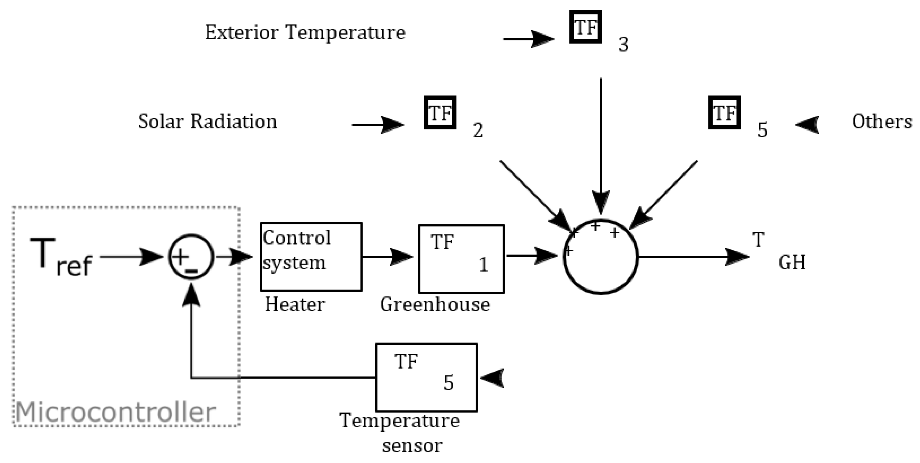
A certain value for the duty-cycle from the PWM signal needs to be converted from a required heat flux so that the internal air temperature stabilizes to the required temperature setpoint. This conversion will be a function of the difference between these two temperatures. This problem can be simplified by identifying transfer functions in a closed loop control system, illustrated by Figure 21.

The control system is usually handled by a PID controller. Its transfer function is equal to the ratio of the controller output to the error in the Laplace domain. In this case, the output is the required heating load (P_H(s)), which will be dissipated by the power resistor, and the input is the absolute value of the temperature error (|T_ref − T_GH| = E(s)). Matlab has a toolbox named System Identification, which estimates an n-order transfer function when certain input and output data are given. Thus, E(s) will be the input (OpenStudio simulation with no heating loads) and P_H(s) will be the output (OpenStudio simulation with a heating load). 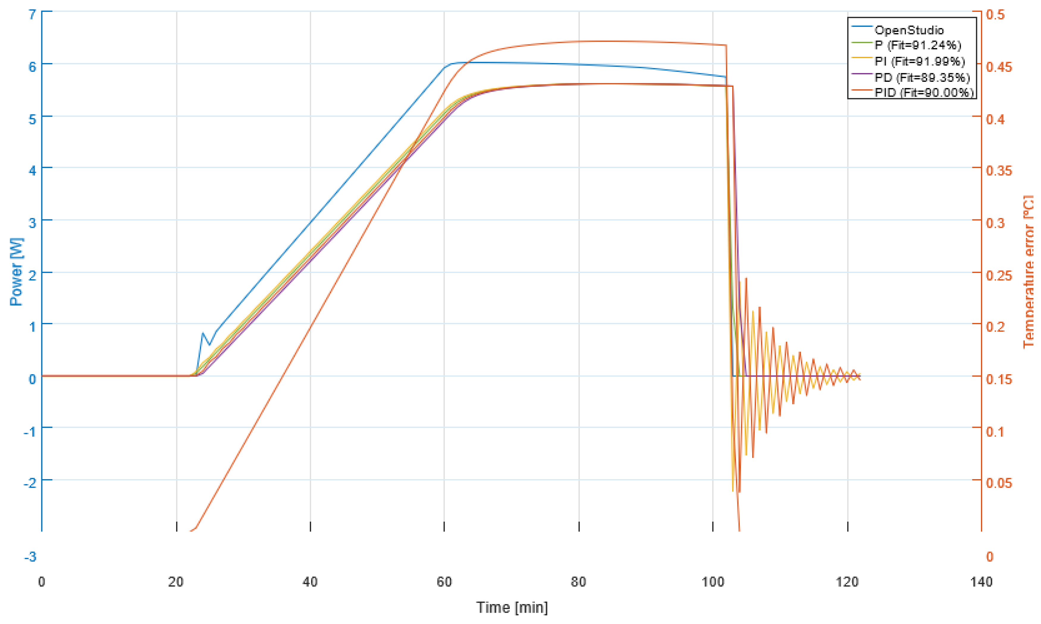Figure 22 shows the temperature error and the required heating load for a previous OpenStudio simulation, during a particular day of the simulation year.

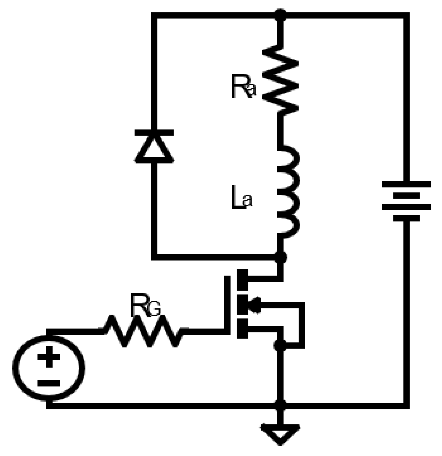
Analysing this figure, the proportional-integral controller has the better fit. In the OpenStudio simulation, the fan had a On/Off behaviour, meaning it would draw its rated power when it would be turned on and so the On/Off behaviour can be replicated with another transistor, with much less strict parameters related to power losses. The most popular and simple way to fix the flyback effect is to add a diode in anti-parallel with the inductive load, usually called a “flyback diode”. Figure 23 shows the usual circuit with this diode present.

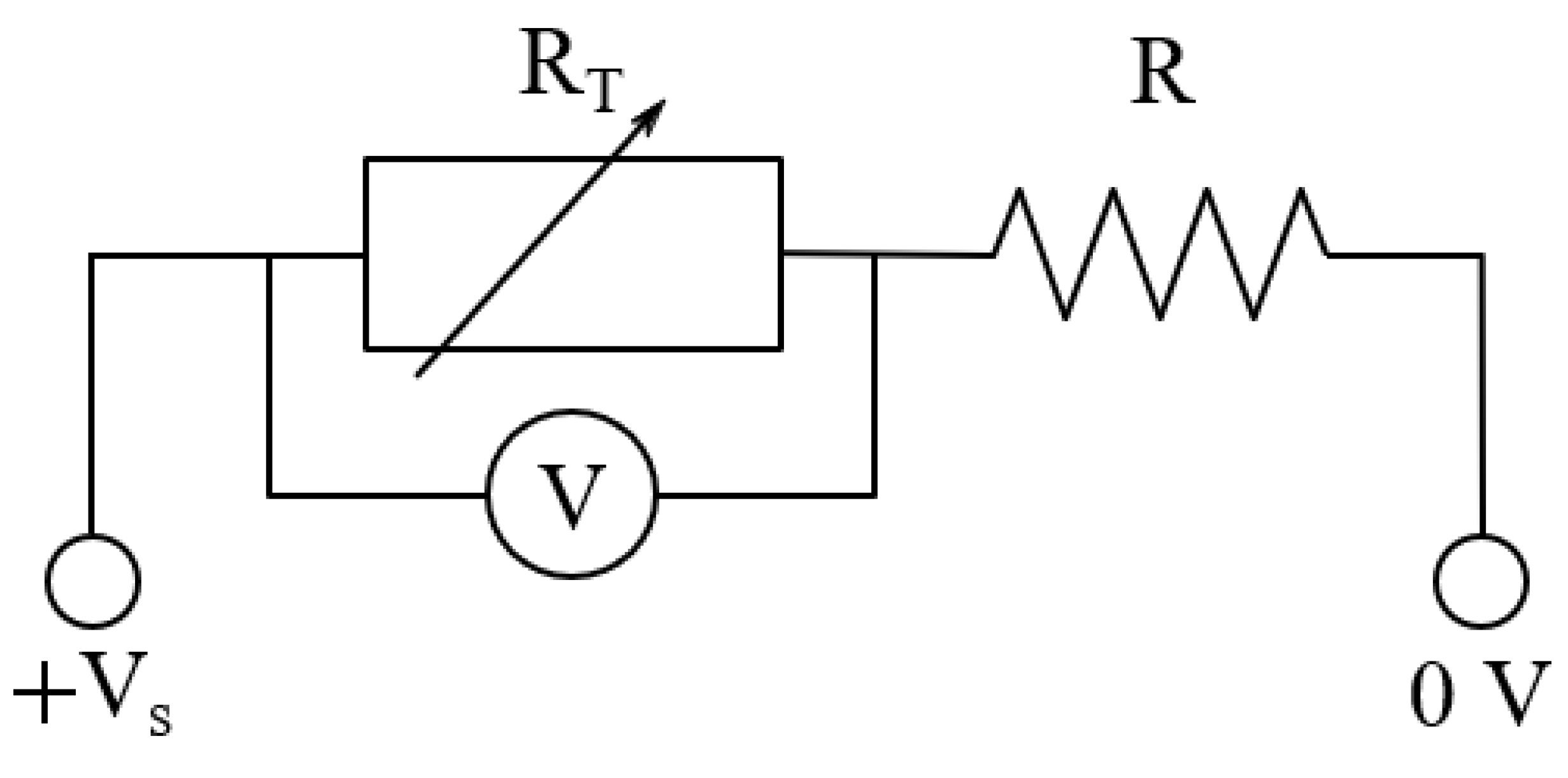
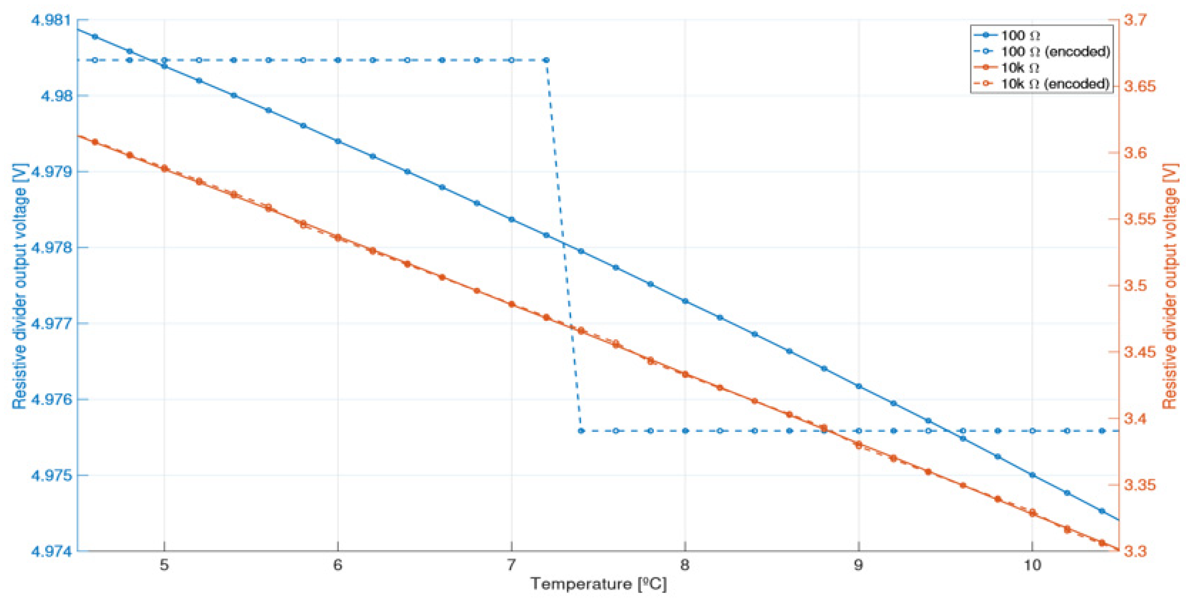
A thermistor is a thermally sensitive resistor composed of semiconductor materials, typically ceramic or polymer. It usually has a negative temperature coefficient with an exponential relationship between the temperature and resistance. Because the electrical property that changes with temperature in a thermistor is resistance and the microcontroller only measures voltages through its analog input pins, a voltage divider is required, in which the thermistor is the variable resistor with the unknown resistance. This requirement is illustrated as a basic circuit in Figure 24.

For certain values of the series resistor, the ADC’s resolution can undershoot/overshoot the original value for a significant amount. To visualize this effect, each original voltage value was encoded using the ADC’s resolution.

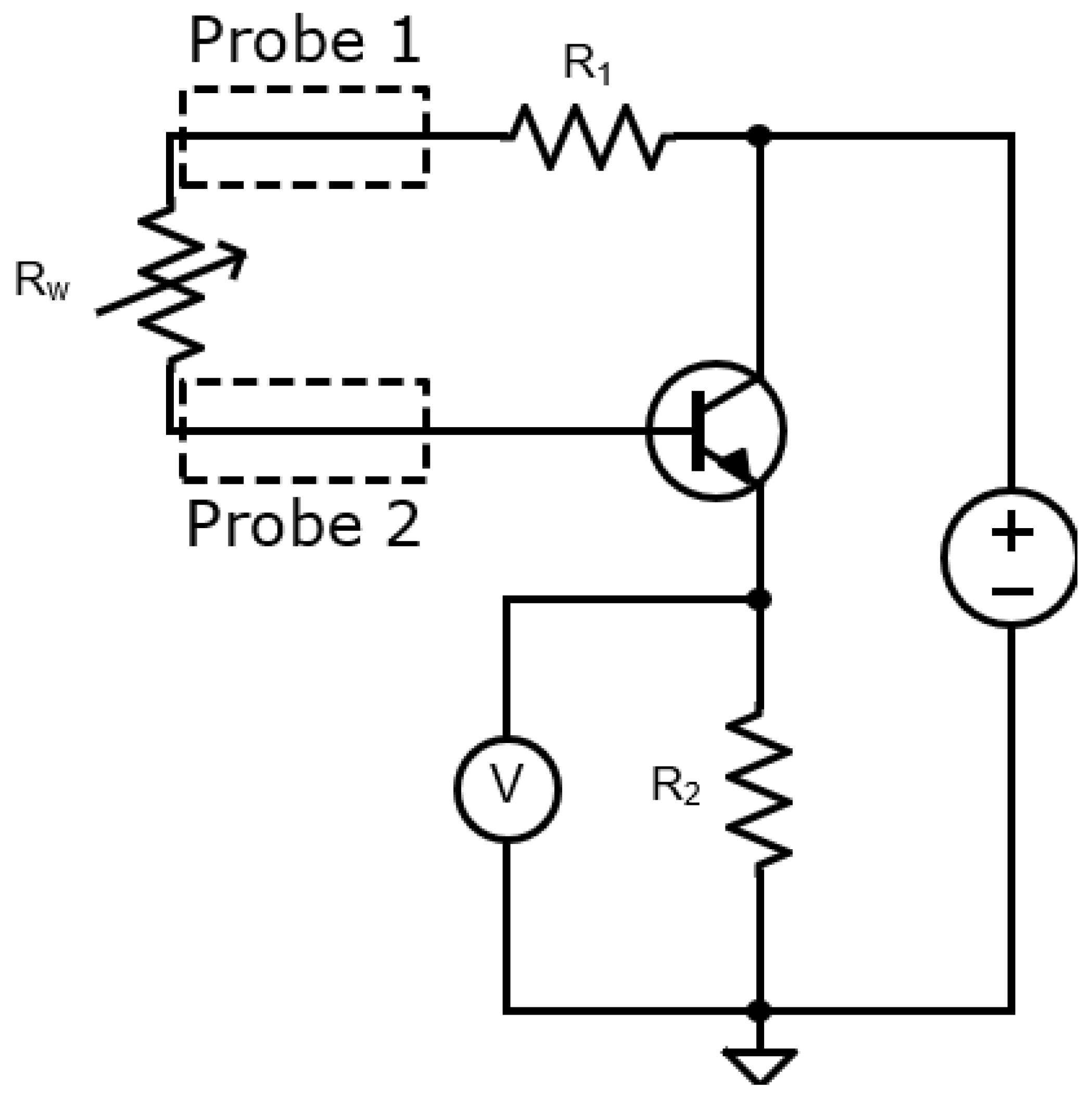
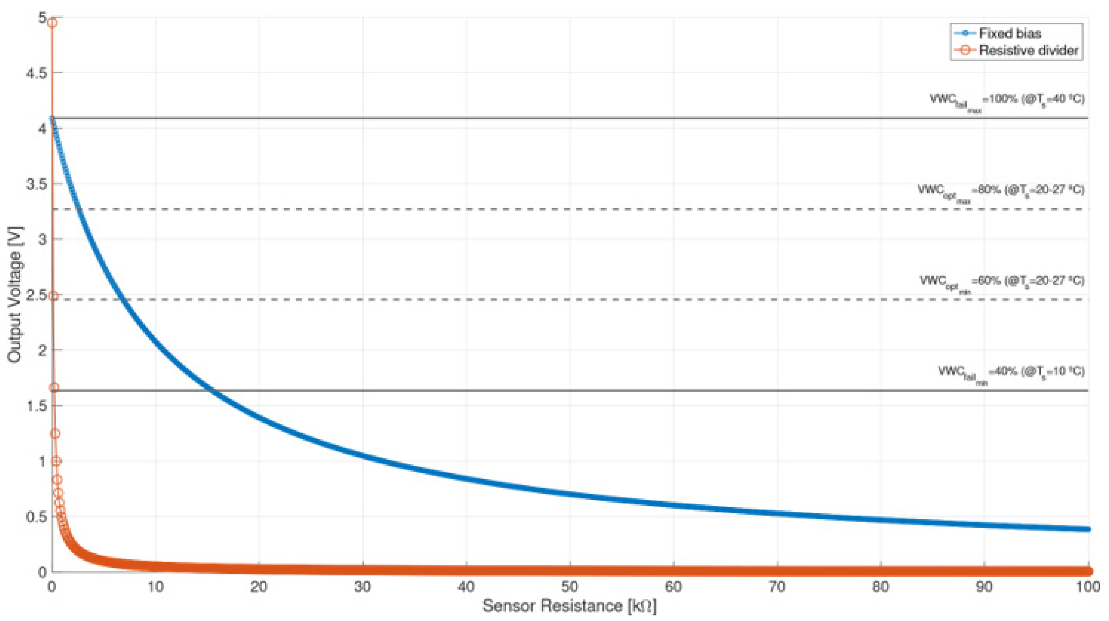
As illustrated, the encoded values for the lowest resistor are heavily mismatched for the main temperature range. There are a variety of different technologies to measure the amount of water in a substance, which rely on measurements of some other quantities. By far the cheapest commercially available hygrometers are resistivity-based soil moisture sensors, which fit in the categorical type of data measurement. Unlike a voltage divider, in which different resistance values (in linear fashion) rapidly decrease the output voltage, the circuits used in these sensors establish a somewhat linear relationship for a certain resistance value range, while not having too small increments for the voltage (effect visualized in Figure 25). This circuit has an NPN transistor in fixed bias with an emitter resistor, pictured in Figure 26.

To visualize the voltage for multiple values of the sensor resistance, the circuit in question was simulated in LTSpice, setting R₁ and R₂ to 100 Ω. Figure 27 shows the simulation result, both for the fixed bias and voltage divider (using a 100 Ω series resistance) circuits.

To transport the water from the reservoir to the end devices of the irrigation, a small, low power, submersible water pump will be utilized, as the amount of water that is required to water the crops is relatively low, considering the volume of soil in the greenhouse. In irrigation management, soil evaporation (E_s) is often seen as “water loss” to the atmosphere, as it cannot directly be used by the crop. This water loss and plant transpiration (T_r) represent what is called evapotranspiration E_T, which is described by Equation (13).

E_T = T_r + E_s

(13)

Thus, the total daily volume of water that is lost is defined as E_T. Considering the worst case scenarios, at maturity on sunny days, tomatoes may need up to 2.7 L/plant/day [9]. Knowing that greenhouse tomatoes need at least a growing area of 4 ft²/plant [10] (around 0.371612 m²), results in 4 tomato plants considering the total growing area, which induces T_r = 10.8 L/day. A study that estimated soil evaporation during the summers of 2010, 2011 and 2012 in southeast Portugal concluded that for wet areas the daily average was 2.41 L/m² [11]. For the total growing area this gives E_s = 4.71 L/day. Thus, the total required volume of water is V = E_T =15.51 L/day. Water pump manufacturers usually give the rated volumetric flux ($\dot{V}$) at a given rated voltage, defined in Equation (14).

$$\dot{V}=\frac{dV}{dt}$$

(14)

For a certain chosen commercially available 4.2 W 12 V water pump, $\dot{V}$ = 4 L/min. With this value, using the previous Equation, it is possible to know how much time it takes to deliver the required volume at such flux, that is around 4 minutes, which is a reasonable amount of time. In OpenStudio, the GHI was used to have a distinction between what was considered night and day for the lighting schedules. Further analysis with Radiance was used to determine illuminance values in the PAR region and, consequently DLI values.

In the real world, there are sensors that measure light in this range, using long and short pass filters, which can be expensive. Fortunately, an article describing an inexpensive apparatus using a TCS34715FN photodiode [12] that can distinguish between red, green, blue and white light, was able to perform comparably to a commercial PAR sensor [13]. By using an algorithm developed by Kuhlgert et al. (2016), PAR light values can be approximated using the outputs of the four light channels obtained from the photodiode [14], described by Equation (15).

PPFD = (W · 0.65) + (R · 1.60) + (G · 2.30) + (B · 0.50)

(15)

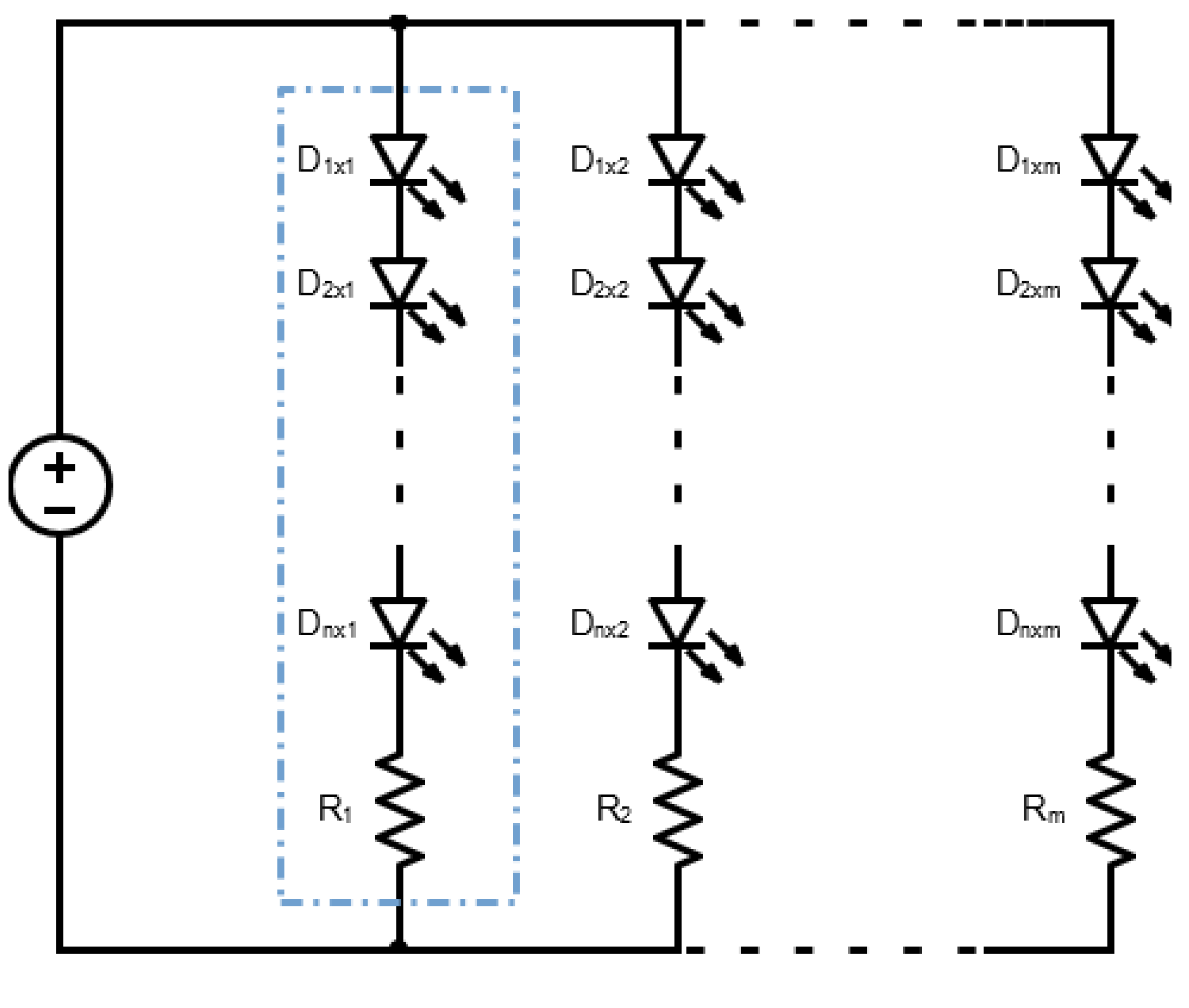
This method provides an easy-to-use, modular, cost-effective, and reliable solution for light intensity measurements. The said sensor comprises a 4 × 4 photodiode array, composed of red-filtered, green-filtered, blue-filtered, and clear photodiodes. For this application, there are commercially available LED strips, containing various LED chips in parallel. Each chip serves as the housing for various LEDs in series, adding the forward voltages (V_F) of each LED to establish the load voltage requirement. These chips also come with a resistor to establish a load current, protecting the LEDs. This combination of different chips with different strip lengths results in a matrix like arrangement considering each LED. Figure 28 shows the equivalent circuit for this type of grouping with voltage supply. The highlighted blue dashed box represents a single chip.

From this, one can deduce the voltage and current of the strip.

$$I_{strip}=m\frac{V}{R}$$

(16)

V_strip = V_chip = n · V_F + I · R

(17)

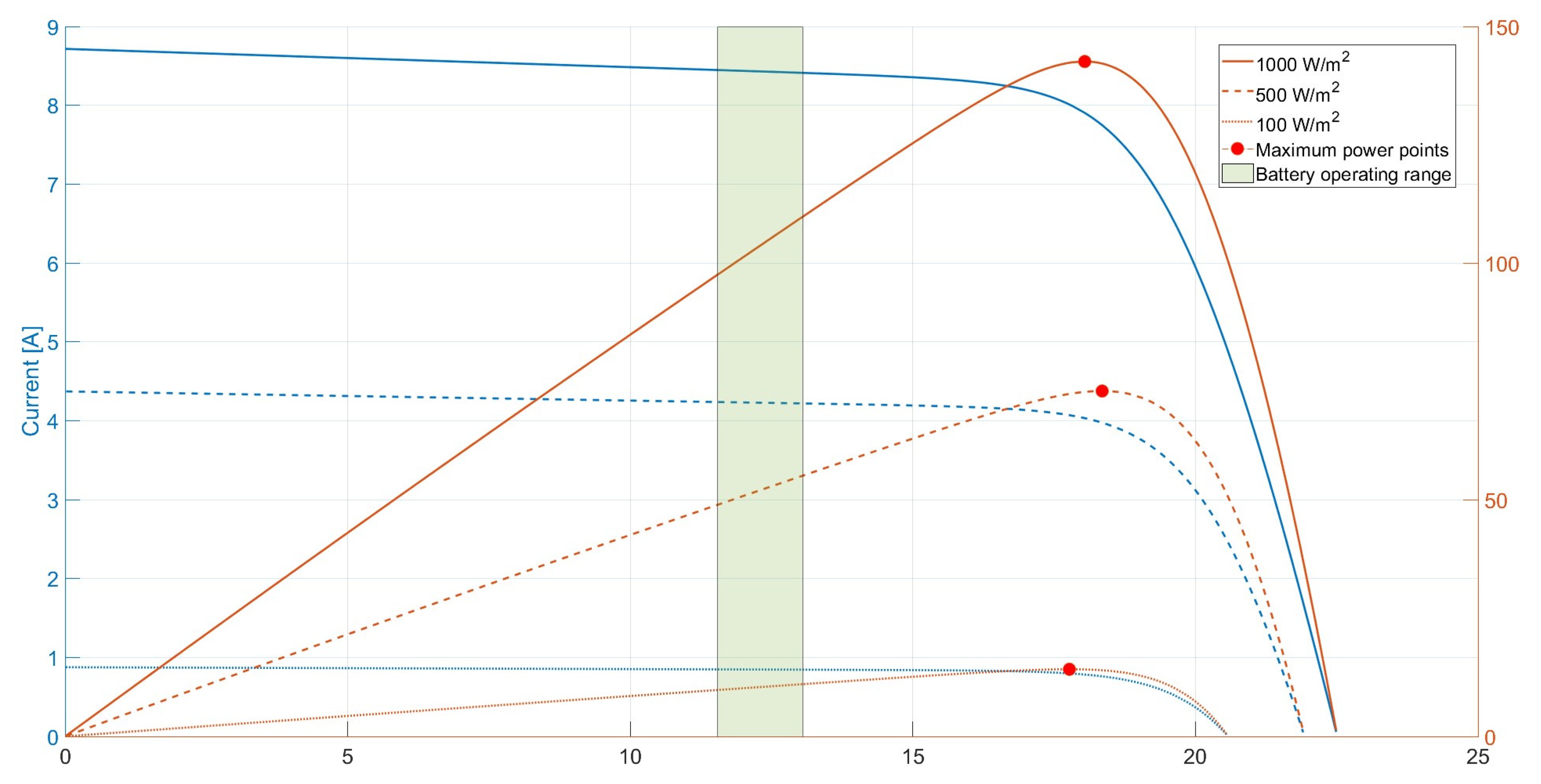
Until now, it was assumed that the solar panel would be directly connected to the battery. For applications where efficiency matters, this is not the best practice, as the solar panel is not a linear device and so its maximum power output is not constant. Figure 29 shows the characteristic curve at various irradiance values, with the battery operating range in a highlighted area.

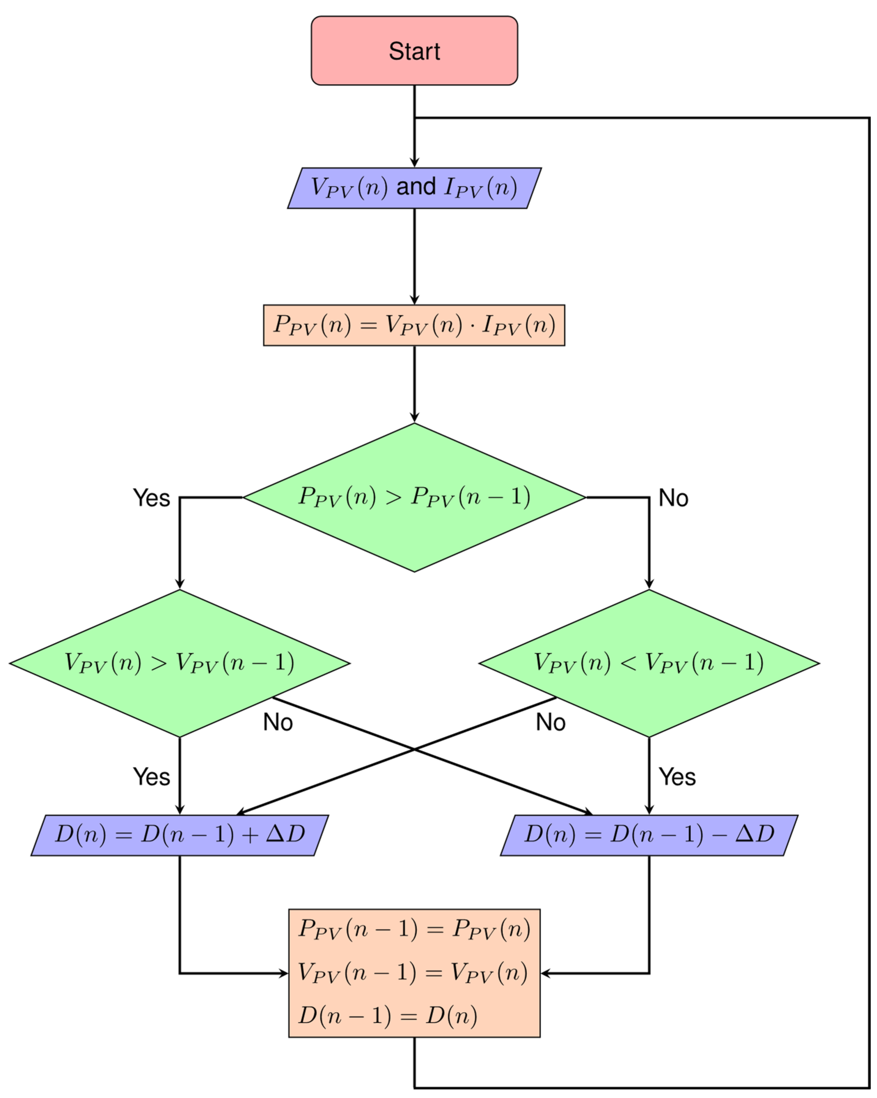
As can be seen, the maximum power points for almost any irradiance value is outside the range of the battery’s voltage. To fix this, a DC-DC converter establishing MPPT is employed. Equation (18) shows the relationship of the necessary duty cycle to implement MPPT.

$$D_{opt}=\frac{V_{BAT}}{V_{P{V}_{MP}}}$$

(18)

Figure 30 shows the flowchart of the chosen Perturb and Observe algorithm.

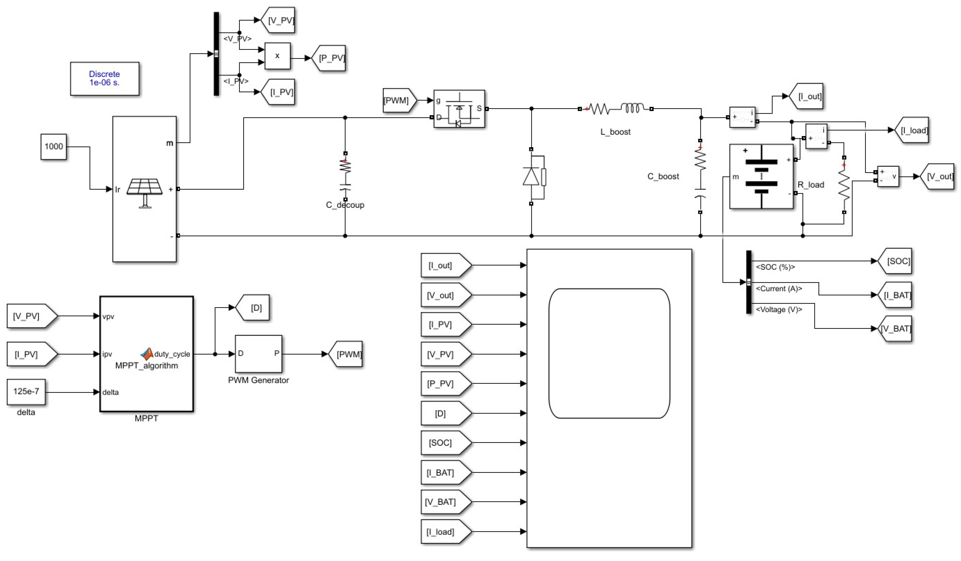
A Simulink model of the system was made using the built-in battery photovoltaic array blocks. The model is illustrated in Figure 31.

Usually, the design of a DC-DC converter is based on a required duty cycle and voltage and current ripples, so that for a given switching frequency (f_sw) the capacitance and inductance can be calculated. For this application, it is not sensible to use such an approach. The output ripples will be much lower, as the charging element is the battery, with a much higher response time than the rest of the components of the buck converter, disregarding the need for high frequency switching. For these reasons, a trial and error approach is executed with this model. 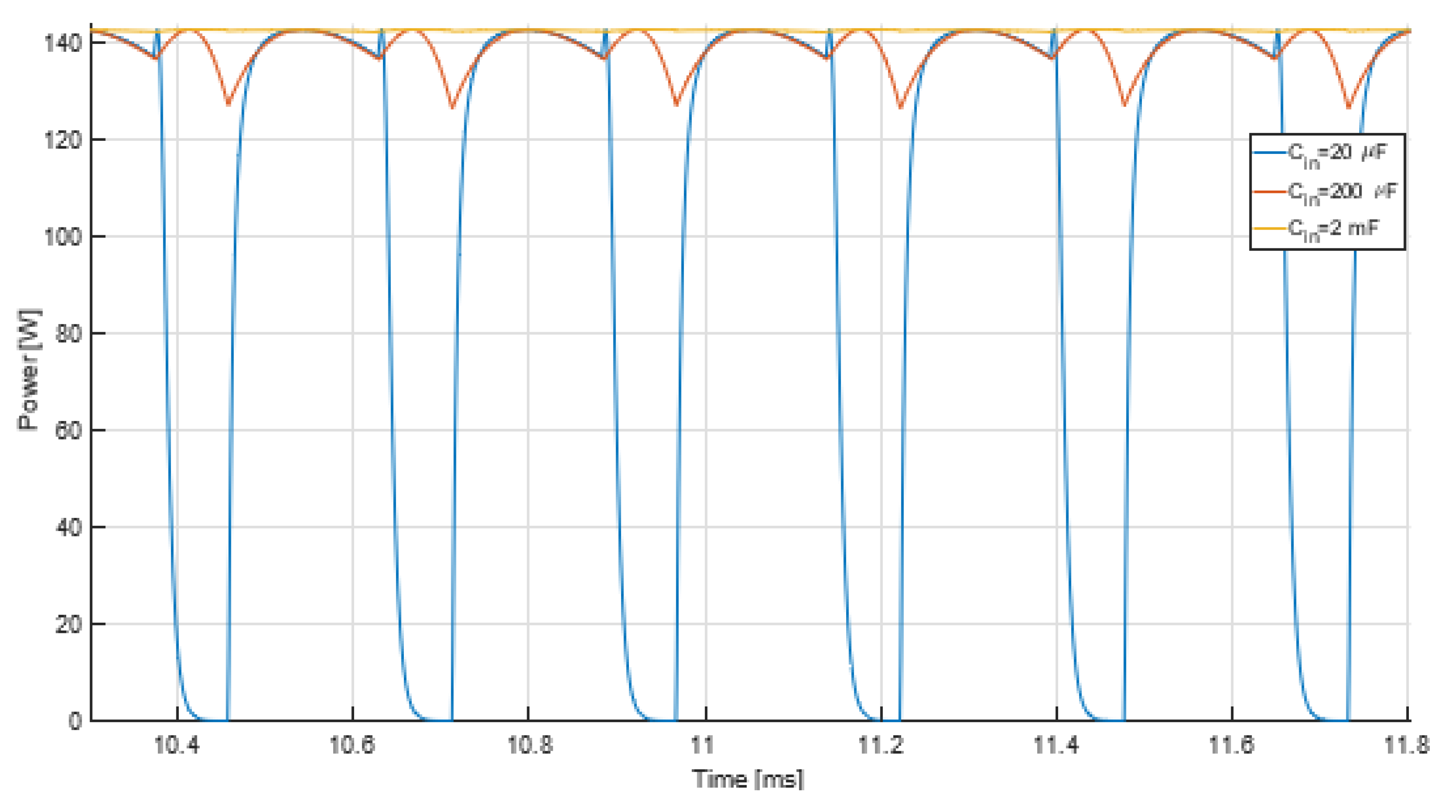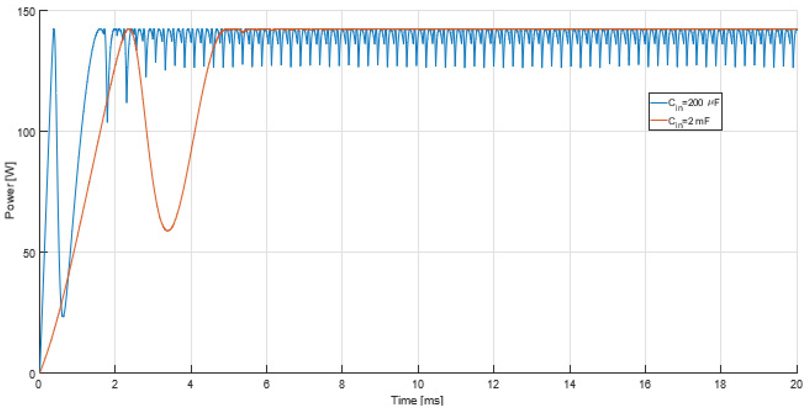Figure 32 and Figure 33 show the final solar array output power of this model.

From these figures, it can be concluded that the PO algorithm is working. The yellow line stays around the maximum power point, with minimal oscillatory behaviour.

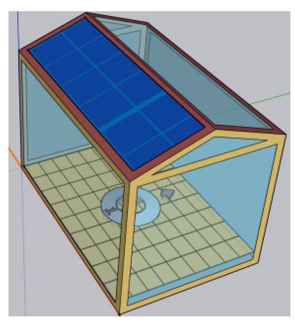
In the next figure (Figure 34), it is possible to see a Sketchup model of the greenhouse.

4. Conclusions

This paper investigated the design and implementation of a greenhouse situated in Lisbon. It was concluded that the best configuration for the greenhouse was an East-West orientation, with an even-span shape, while using a PC sheet with a 9.2 mm air-gap thickness as the glazing construction. This combination resulted in a total ideal annual heating and cooling energy of 0.2451 and 10.9030 MJ, respectively.

In the transition from ideal air loads to real world loads, using OpenStudio, a roof opening serving as natural ventilation on the east or west side resulted in the same cooling effect. With an opening area of 0.637 m² this resulted in summer internal peak temperatures going from 60 to 30 °C. With additional reflective shading using aluminium sheets, the internal temperatures were able to reach thermal equilibrium with the outside temperature. A unit heater composed of a 75 W heating coil with a 50 CFM heating fan managed to maintain the internal temperatures to the minimum temperature established for the crops during the night.

Radiance was used to establish an illuminance map in the growing area of the greenhouse, which was used to create a light schedule for OpenStudio using 30 W light load, based on a previously set target DLI for the crops. This load would be composed of red and blue LEDs, as they have nearly 4 times the effectiveness in the DLI when compared to natural sunlight, for the same irradiance. Figure 28 shows the result of the energy consumption of these loads.

Using OpenStudio, energy generation with a 150 W photovoltaic array was also simulated, concluding that using a tilt angle more appropriate for the winter season and an azimuth angle towards the south was the better decision.

Secondly, two 3.3 Ω, 50 W wire-wound resistors in parallel controlled by PWM were selected as the heating element for the heating subsystem, with a power MOSFET serving as the switching element, justifying the use of a gate resistor. A closed loop system with individual transfer functions was identified to determine the better transfer function for the PID controller. This estimation was done through Matlab’s System Identification toolbox, using previous OpenStudio data, with a 91.99% data fitting percentage. For the heating fan, the inductive flyback effect was described, using a flyback diode as the solution. For the temperature sensor, a thermistor with tight tolerances was chosen, choosing the best series resistor to minimize encoding errors.

For the irrigation subsystem, a low cost resistive soil moisture sensor was chosen as the VWC sensor, stating the required calibration procedures. The circuit of this sensor was also described, for the purpose of analysing the sensitivity across a range of resistive values. As the actuator, a submersible 12 V water pump was chosen, switched by a MOSFET. 15.51 L/day was the estimated worst case scenario for the required volume of water, for the chosen crops. For this scenario, the pump would take 4 min to transfer the water. It was also concluded that the accuracy of the control timer is irrelevant, considering the volume of the growing area.

For the lighting subsystem, an algorithm was used to convert inexpensive photodiode light measurements for individual colors into useful PAR radiation, which is used to calculate the DLI. As the actuator, 75 a custom sized 12 V 30 W LED strip was chosen, with 4 blue and 8 red chips, switched by a MOSFET.

Finally, the battery charging method was described and derived, using PO as the MPPT algorithm.

To sample the photovoltaic array’s voltage and current, a voltage divider and a Hall sensor, respectively, were chosen. With a buck converter to step down the voltage of the photovoltaic array, a Simulink model was successfully implemented, with constant maximum power available from the panel, mimicking the duty-cycle digital control behaviour of the microcontroller. The resulting voltage and current ripple was around 0.0025% (due to the battery’s transient) and 6%, respectively.

It can be concluded that the combination of all these systems can create a sustainable environment for the tomatoes, while having minimal power losses, satisfactory operational conditions for all of the electrical systems and reduced cost.

5. Future Work

Below are what the authors consider to be the most important issues for future investigation:

• Site shading. This can reduce energy generation from the photovoltaic array by a considerable amount, especially during the winter season.
• Different energy modelling software. Each software has its own thermal and fluid dynamics and weather models, which could make a measurable difference on the estimated loads.
• Range of crops. For simplicity sake, a single tomato crop was studied. A variety of crops would give different load estimations, depending on their needs.
• More greenhouse configuration scenarios. The presented scenarios were not exhaustive, being decided by their popularity in research articles and market availability/cost.
• Forced ventilation. During different simulations instances, forced ventilation for cooling was implemented. Unfortunately, it made no difference in the internal temperature of the greenhouse, even with absurd levels of airflow. Different methods and different software could further reduce the summer peak temperatures using this cooling method.
• Physical implementation of this project. There a lot of hidden variables that were not discussed in this paper that could impact a greenhouse: temperature gradients inside the greenhouse, heat leakages, organic heat loads, etc. A revision of the controller transfer function would have to be made as well, as the available data had a 5 min time interval, which could bring inaccuracies.