Revamping Optimization of a Pressure Piping System Using Artificial Neural Networks

Abstract

The paper proposes a new methodology for revamping design and optimization of a process piping system. Starting from ASME B31.3 Process Piping prescriptions for stress analysis, a nonlinear model is built to express the relationship between stress distribution generated by expansion and sustained loads (pressure, weight) and the geometry and routing of the pipeline, focusing on geometric parameters of expansion loops. The number of design variables affecting stress distribution over the pipe, together with the constraints to be respected, would make it hard to formulate an optimization procedure based on deterministic methods. This problem is overcome by applying a Feed Forward Neural Network, backpropagation trained, which makes it possible to interpolate a non-linear and multidimensional relation over a domain enclosed within the boundaries of a training set. Prediction of code stresses is obtained through the fitting of an artificial neural network for each examined loadcases. Network parameters are tuned offline, starting from a set of data obtained by finite element numerical simulation. As a result, an optimal geometry for expansion loops is found, allowing to revamp pipe routing by halving loops number and keeping code stress within the allowable limits.

1. Introduction

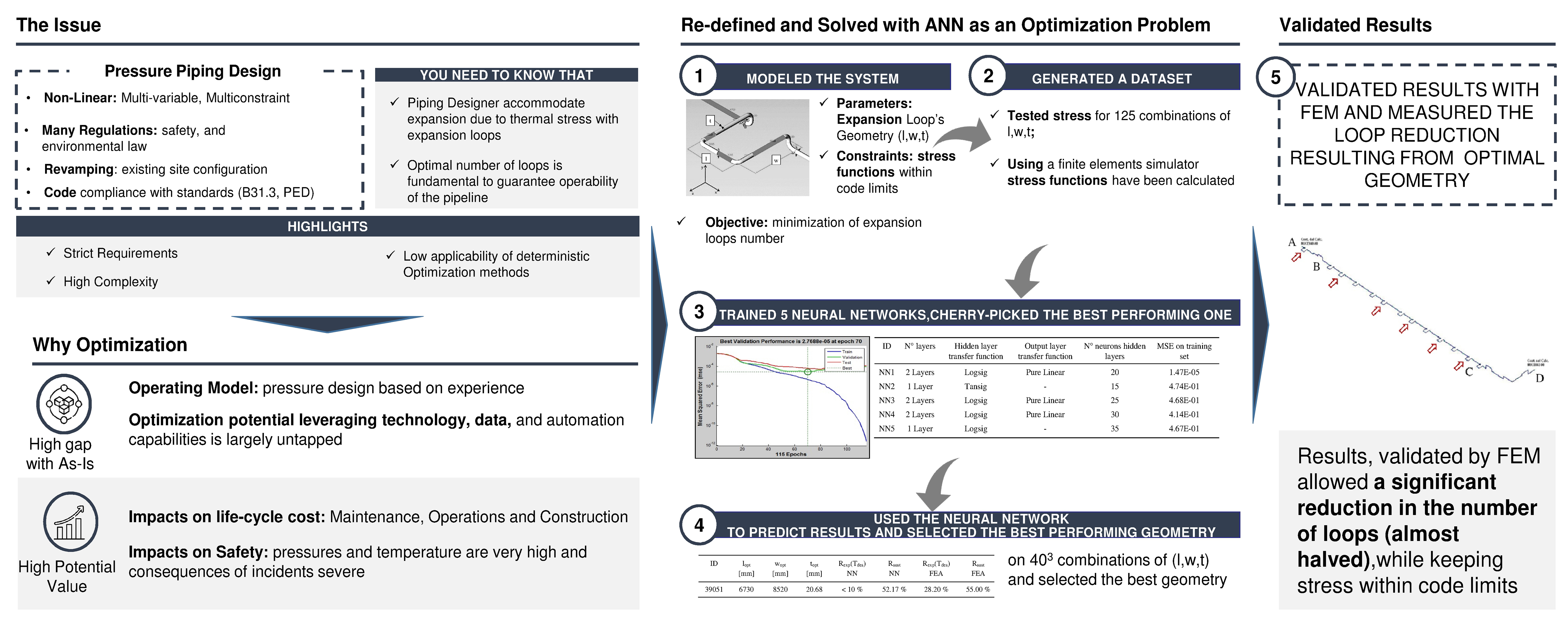
Technological knowledge has been advancing since the existing plants were designed. In addition, economic, environmental, regulatory conditions are dynamic and change over time. Consequently, a wide variety of reasons may emerge to improve, upgrade, adapt an existing plant, or a part of it. When new needs arise, such as to reduce the impact of the process on the environment, to improve the safety, reliability, and flexibility of the process, retrofitting of some equipment is required [1,2]. When instead more radical changes have to be made, such as to use feed of different quality or alternative feed, to meet new specifications of product or produce new products, a real reconversion of the systems becomes necessary, and the revamping of a part or of the whole plant must be planned [2,3].

It is precisely that which one occurs more and more frequently today for petrochemical plants. The increase in fuel price and environmental protection pressure, and the subsequent decrease in oil refined products demand in the long-term oil and gas industry outlook, promote large investment for petrochemical companies to switch their production toward more profitable and sustainable products. Therefore, the plants need to be reconverted for the production of alternative energy sources. This requires restoration of the industrial sites, and the rearrangement of plants through a series of revamping interventions, with the aim of avoiding excessive disposal and shutdown costs.

Piping systems are particularly sensitive to this problem, as they form the backbone of any type of process system, and are composed of a large number of elements. Furthermore, the failure of just one of their components can cause unwanted plant shutdowns, or even worse, severe problems to public health and safety.

In revamping interventions, the introduction of optimization methodologies is essential when it is required that plant lines to be reconceived, and suitably redesigned, in addition to meet new process requirements, should:

• Avoid interference with other pipes, structures, and in general with other existing equipment;
• Facilitate maintenance operations;
• Respect both the current safety and the environmental law;
• Cause stress conditions within the code requirements.

In fact, failure of piping systems can have insidious adverse effect on their safety and reliability. Piping failure frequency in a particular system is an important input parameter to probabilistic safety assessment, and in operating plant it is of great interest to evaluate failure rates and investigate their departure from generic reference values [4]. Estimates of pipeline failure frequencies are typically derived from reports on incident statistics. The most recent data relating to the European context made it possible to estimate a failure frequency over the entire period 1970–2019 equal to 0.29 per 10³ km·year [5]. They also highlighted how the causes of pipeline accidents are diversified, and determined by multiple factors (natural causes and geotechnical phenomena, external interference and third party actions, material/construction causes, corrosion phenomena, unknown causes).

Between them, construction defects and material failures typically constitute a significant share in failure cause distribution, being the wall thickness a key feature for its potential effects on different failure mechanisms [6]. In general, piping reliability is dependent on many construction factors, being the main reliability-related inclusive of, but not limited to, diameter and wall thickness, mechanical and metallurgical behavior of materials, configuration of piping, methods of fabrications and welding. Wall thickness, material, and operating pressure, in addition to the location, are considered key factors for failure classification in gas pipelines [7]. This highlights the importance in pipeline design of balancing all these factors in the best possible way, acting on the design variables in order to guarantee constructive efficiency and system safety.

ASME B31.3 Process Piping code [8] have been introduced expressly to state the requirements for effective stress analysis in piping design for process industry, and guarantee a high level of safety to the construction solutions adopted. Each pipe branch is considered as a hollow tubular element for fluid transfer, subjected to internal and external pressure thermal conditions, and other loading conditions, which create displacement and stress at the fittings, bends, laps, and branch connections.

One of the major aspects in stress analysis of piping system is the expansion of pipes, generally due to high temperature of fluid being transported from one point to another, and to the difference of the surrounding temperature. The corresponding addition of length creates high loads and moments on the fixed points (i.e., the points with zero displacement), such as nozzles and anchors. Furthermore, elbows of the pipe are subjected to the maximum expansion displacement due to space availability.

In oil and gas piping lines this aspect is enhanced by the high temperatures of the operating fluids, and combined with the high pressures, it entails severe condition in stress distribution, as demonstrated by study on thermo-mechanical coupling effect at high temperature [9].

Hangers and expansion joints, which use springs to reduce the loads at the elbows of the pipes, are frequently used: the formers absorb expansion along a vertical line only; the latter can compensate for all the axial expansion, but requires special fittings and supports. Furthermore, such solutions are restricted by high price. So, the most effective and sustainable approach to mitigate the high stresses due to the constraints of piping system to the expansion consists in changing the routing of the piping system by using expansion loops. However, they require extra space, supports, bends, and additional structure, so their geometry and number, and the supports, need to be optimized. With this purpose, a few previous works have proposed optimization analysis concerning the expansion loop dimensions and the number of supports, by using commercial software for pipe stress analysis [10,11].

The aim of this paper is to provide a method to optimize the main geometric parameters of expansion loops in high-pressure pipeline design, to be used in revamping optimization of piping systems. A nonlinear model is proposed to express the relationship between stress distribution generated by expansions and sustained loads (pressure, weight) and the expansion loops geometry and routing of the pipeline. The high number of design variables affecting stress distribution over the pipe, according to ASME B31.3 Process Piping code, together with the constraints to be respected, would make it hard to formulate an optimization procedure based on deterministic methods. This problem is overcome by applying a feed forward neural network, backpropagation trained, which makes it possible to interpolate a non-linear and multidimensional relation between design parameters and stress conditions, over a domain enclosed within the boundaries of a training set. Numerical simulation by the specialized finite element-based software for piping stress analysis Caesar II (Hexagon AB, Stockholm, Sweden) has been used to assess the stress behavior of the piping system as the variables of the optimization problem vary, and to obtain the data for network parameters tuning.

2. Models and Methods

2.1. Stress Analysis Calculation According to ASME B31.3 Code

High-pressure steam pipelines are among the most demanding design challenges. The internal pressure and the boundary constraints generate longitudinal, circumferential, and radial stresses. If the corresponding equivalent stress exceeds a critical value, the failure of the piping could typically occur at the brunch connections. Expansion loops give the piping system the right flexibility to accommodate the strains and stresses without exceeding the allowable stress of the material.

Different loadcase conditions can be considered in stress analysis for piping design. In all cases, according to the ASME B31.3 Process Piping code [8], the corresponding code stress S_(LC) for loadcase LC must not exceed the allowable stress SA, specified in tables based on used material and the operating temperature.

The stress ratio R_(LC), which is defined as the percentage ratio of the code stress S_(LC) to the allowable stress of the material S_A, is used to determine the piping locations with critical stress condition, and the acceptable range of stress within the piping system:

$${\mathrm{R}}_{\left(\mathrm{LC}\right)}=\frac{{\mathrm{S}}_{\left(\mathrm{LC}\right)}}{{\mathrm{S}}_{\mathrm{A}}} \times 100$$

(1)

Between the primary loadcases, sustained case and expansion case will be focused here:

• Sustained case takes into account the loads due to pressure, pipe and insulation weight, and fluid density. Sustained stresses consist in the stresses corresponding to the longitudinal loads, bending moments, and internal pressure.
• Expansion case focuses the expansion of the pipe under the temperature effect and the reactions at the fixed points (where zero displacements occur). With this regard, failure typically occurs due to high stresses. The expansion loops are used precisely to accommodate the expansion of the pipe in the axial direction without exceeding other design constraints.

The code stress S_(LC) is required to remain always lower than the allowable stress S_A under any circumstances for operating conditions. In flexibility stress analysis, the code stress S_(LC) is the displacement stress range S_E, which is defined taking into account the contributions of axial, bending, and torsional displacement stress ranges:

$${\mathrm{S}}_{\mathrm{E}}=\sqrt{{\left({\mathrm{S}}_{\mathrm{b}}+\left|{\mathrm{S}}_{\mathrm{a}}\right|\right)}^2{ + 4\mathrm{S}}_{\mathrm{t}}^2}$$

(2)

The bending stress range due to displacement strains S_b is expressed by

$${\mathrm{S}}_{\mathrm{b}}=\frac{\sqrt{{\left({\mathrm{i}}_{\mathrm{i}}{\mathrm{M}}_{\mathrm{i}}\right)}^2+{\left({\mathrm{i}}_{\mathrm{o}}{\mathrm{M}}_{\mathrm{o}}\right)}^2}}{\mathrm{Z}}$$

(3)

where M_i and M_o are the in-plane and out-plane bending moments, respectively, at the branch connections (elbows, bends, tees); i_i and i_o are the in-plane and out-plane stress intensification factors, respectively (they depend on shape and geometric parameters of bend or tee to which they refer); Z is the section modulus of the pipe.

The axial stress range due to displacement strains S_a is expressed as a function of the axial force F_a, the cross-sectional area of pipe A_p, and the axial stress intensification factor i_a:

$${\mathrm{S}}_{\mathrm{a}}=\frac{{\mathrm{i}}_{\mathrm{a}}{\mathrm{F}}_{\mathrm{a}}}{{\mathrm{A}}_{\mathrm{p}}}$$

(4)

The torsional stress range due to displacement strains S_t in Equation (2) is expressed as a function of the torsional moment M_t, and the torsional stress intensification factor i_t:

$${\mathrm{S}}_{\mathrm{t}}=\frac{{\mathrm{i}}_{\mathrm{t}}{\mathrm{M}}_{\mathrm{t}}}{2\mathrm{Z}}$$

(5)

ASME B31.3 states that the code stress SE should not exceed the value of the allowable displacement stress range S_A. It is defined according to the following conditions:

$${\mathrm{S}}_{\mathrm{A}}=\mathrm{f}\left(1.25{\mathrm{S}}_{\mathrm{c}}+0.25{\mathrm{S}}_{\mathrm{h}}\right){ \mathrm{for} \mathrm{S}}_{\mathrm{h}}{ < \mathrm{S}}_{\mathrm{L}}$$

(6)

$${\mathrm{S}}_{\mathrm{A}}=\mathrm{f}\left[1.25\left({\mathrm{S}}_{\mathrm{c}}{+\mathrm{S}}_{\mathrm{h}}\right){- \mathrm{S}}_{\mathrm{L}}\right]{ \mathrm{for} \mathrm{S}}_{\mathrm{h}}{ > \mathrm{S}}_{\mathrm{L}}$$

(7)

where S_c and S_h are the basic allowable stress at minimum metal temperature (cold condition) and maximum metal temperature (hot condition) expected during the displacement cycle under analysis, respectively, and f is the stress range reduction factor, which depends on equivalent number of full displacement cycles during the expected service life of the piping system.

The term S_L is the stress due to sustained loads (pressure and weight), defined by an equation in the same form of (2), where in this case S_b, S_a, and S_t are the bending, axial, and torsional stresses due to sustained loads, respectively.

In sustained case, which does not concern with expansion effects, the allowable stress S_A is expressed by:

$${\mathrm{S}}_{\mathrm{A}}=\frac{{\mathrm{S}}_{\mathrm{h}}}{{\mathrm{E}}_{\mathrm{c}} \mathrm{W}}$$

(8)

where S_h is the basic allowable stress at maximum metal temperature (hot condition), E_c is the casting quality factor (for cast piping materials), and W is the weld joint strength reduction factor.

As the loadcase condition varies, the generalized expression of the stress ratio in Equation (1) will be developed by substituting the corresponding expressions of the code stress S_(LC) and the allowable stress S_A.

Finally, the condition of pipe minimum thickness for pressure design must always be respected. According to the ASME B31.3 code, when t_p < D/6, being t_p the pressure design thickness and D the outside diameter of pipe, the minimum required thickness t_m is expressed by:

$${\mathrm{t}}_{\mathrm{m}}{ = \mathrm{t}}_{\mathrm{p}}+\mathrm{c}$$

(9)

where c is the sum of the mechanical allowances (thread or groove depth), plus corrosion and erosion allowances. The pressure design thickness t_p is expressed by:

$${\mathrm{t}}_{\mathrm{p}}=\frac{\mathrm{P} \mathrm{D}}{2\left(\mathrm{S} \mathrm{E} \mathrm{W}+\mathrm{P} \mathrm{Y}\right)}$$

(10)

where P is the internal design pressure, S is the basic allowable stress for pipe material, E is the quality factor, W is the weld joint strength reduction factor, and Y is a dimensionless factor which varies with temperature and material. In this type of expression, the term E can be the casting quality factor E_c or the longitudinal weld joint factor E_j; if a component is made of castings joined by longitudinal welds, both casting and weld joint quality factors are applied, and their product becomes the equivalent quality factor.

2.2. Problem Statement

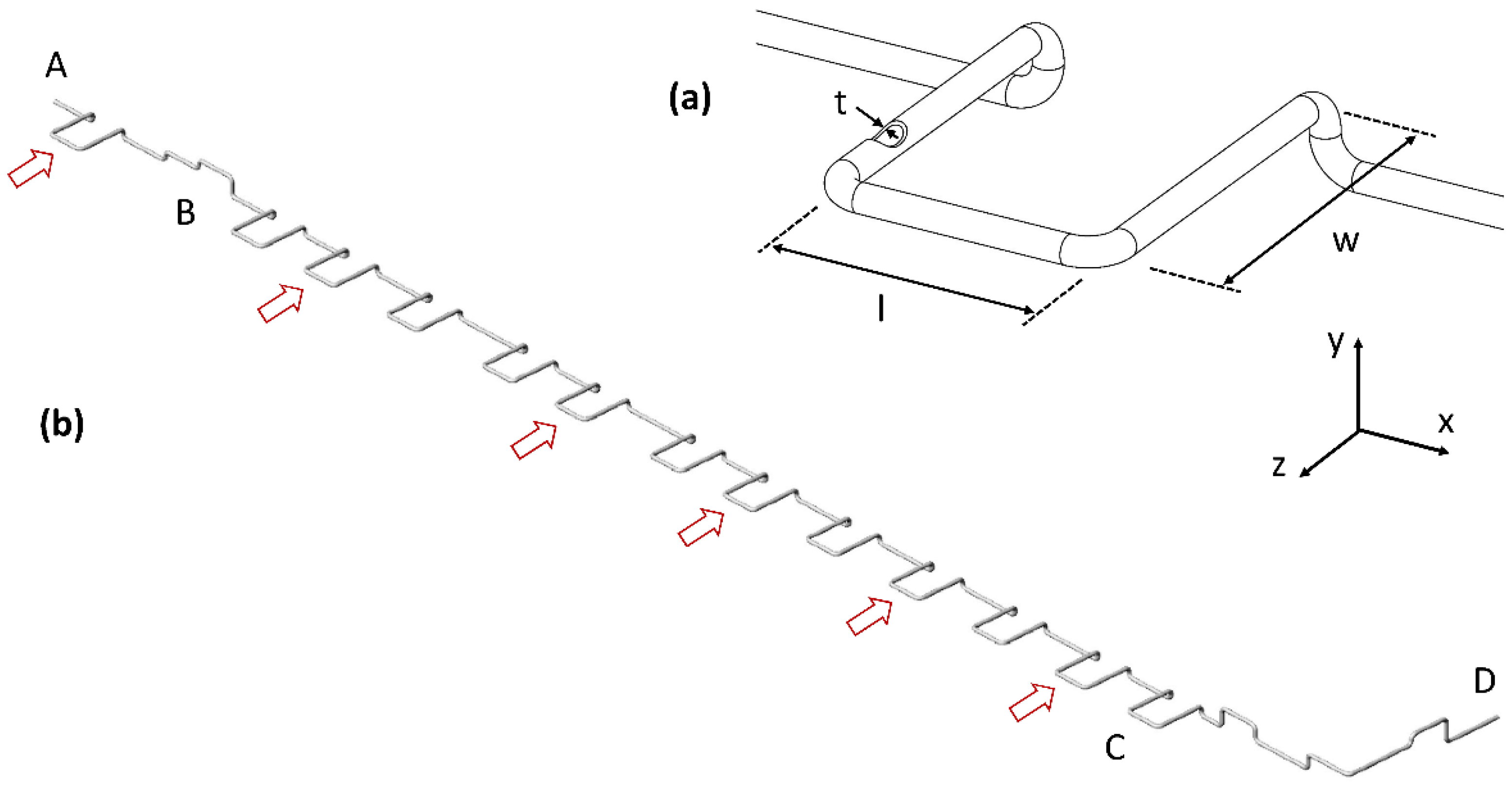
Given a piping system running along a certain path which connects two or more fixed points, let (l, w, t) be leg length, width, and wall thickness of the pipe in an expansion loop, as shown in Figure 1a. In general terms, in expansion loops the pipes can be routed in both the directions perpendicular to the main direction of the pipeline, obtaining a six-elbows loop developing along all the three axes x, y, z (such as in Figure 1a); or only in one direction perpendicular to the pipe, obtaining a four-elbows loop developing on the plane xz. The former is the most commonly used, the latter instead is used when less flexibility is needed or some process constraints prevail. However, when the vertical leg of the six-elbows loop is limited, as in the case analyzed, its effect on stresses distribution is limited and can be neglected, and no further geometric feature is needed to be added in the vector of variables to be optimized. With these premises, the expansion loops have been modelled by the six-elbows layout in Figure 1a, and the corresponding three-variables vector (l, w, t).

Trying to find an optimal set for (l, w, t) it is necessary to model the relationship between stress ratio and expansion loop geometry:

$${\mathrm{R}}_{\left(\mathrm{LC}\right)}{ = \mathrm{R}}_{\left(\mathrm{LC}\right)}\left(\mathrm{l},\mathrm{w},\mathrm{t}\right)$$

(11)

The high number of design variables affecting stress distribution over the pipe, introduced in the model for stress analysis of Section 2.1, together with the constraints to be respected, would not allow to define the relationship (11). This problem can be overcome by using a suitable artificial neural network (ANN) that makes it possible to interpolate a non-linear relation over a domain enclosed within the boundaries of a training set.

Let be routing, constraints on expansion loop geometry, and loadcase conditions the model parameters; the response variables are the stress ratios expressed by Equation (1), for each of the examined loadcase conditions:

• R_exp (T_des) and R_exp (T_op), stress ratios for expansion loading conditions at design temperature and operating temperature, respectively;
• R_sust, stress ratio for sustained loading condition.

On the one hand optimization process can be focused on the vector of variables (l, w, t) corresponding to minimum R_exp (T_des), since it results to be a condition more critical compared to R_exp (T_op). On the other hand, improving the resistance of the pipeline, the number of loops necessary to absorb the expansion is reduced with a consequent decrease of sustained loads over the pipe.

Therefore, the optimization model presented in this work uses as objective function the following:

$$\varnothing =\min \left[{\mathrm{R}}_{\exp }\left({\mathrm{T}}_{\mathrm{des}}\right)\right]$$

(12)

The examined pipeline is a high-pressure steam line, which is a part of a system serving a Combined Cycle Gas Turbine (CCGT) for power generation, and is schematized in Figure 1b. In

Table 1. Line data.

PED category	III	Material	CS A106 Gr.B
Rating	600#	Size	16″
Design pressure	4.5 MPa	Led length lo	6130 mm
Design temperature	420 °C	Leg width wo	8500 mm
Hydrostatic test pressure	6.75 MPa	Wall thickness to	17.48 mm
Operating temperature	360 °C	Corrosion allowance	1.27 mm
		Insulation thickness	160 mm

main data for existing pipeline (Pressure Equipment Directive PED category, rating, design conditions, operating conditions, material and size, expansion loop current geometric parameters) are reported.

In the choice of the discrete points to investigate, “feasibility” and “proximity to as-is” constraints were considered, to be intended as follows:

• Feasibility: feasible discrete points were chosen, as the dimension used can be found in standard components available on the market (this type of constraint has been applied particularly to thickness t).
• Proximity to actual design: artificial intelligence starts from the configuration already on place to find an optimal solution.

The discrete domain that satisfies the previous constraints is obtained by assigning five levels to each variable in the neighborhood of a given configuration (l, w, t). Therefore, the following sets of values for each term of the variables’ vector are defined:

• l ∊ (5930, 6130, 6330, 6530, 6730) [mm]
• w ∊ (8500, 8600, 8700, 8800, 8900) [mm]
• t ∊ (15.88, 16.66, 17.48, 19.02, 20.62) [mm]

Generally, the approach for a revamped design will be different from a new design, as it will have many existing constraints, set by the current design. Chiba et al. [12] proposed genetic algorithms for re-designing the support system of a pipeline starting from current configuration while Fong et al. [13] used Design of Experiments techniques to search for an optimal configuration starting from a sample obtained by means of a FEA. Following this, a 5³ factorial design consisting of 125 loops geometries in the neighborhood of the current configuration (l_o, w_o, t_o) has been generated and synthesized in

Table 2. Factorial design and FEA outputs.

ID	ID FEA	l [mm]	w [mm]	t [mm]	Rexp (Tdes)	Rsust
1	52	5930	8500	17.48	44.9%	66.8%
2	13	6330	8700	15.88	42.3%	65.8%
3	43	6330	8800	16.66	41.4%	63.6%
4	20	6730	8800	15.88	41.6%	65.9%
5	90	6730	8700	19.05	40.5%	58.0%
6	3	6330	8500	15.88	41.6%	60.8%
7	17	5930	8800	15.88	43.9%	71.3%
8	11	6130	8700	15.88	42.4%	65.8%
9	88	6330	8700	19.05	41.5%	61.5%
10	100	6730	8900	19.05	39.4%	58.0%
…	…	…	…	…	…	…
29	125	6730	8900	20.62	38.7%	55.1%
…	…	…	…	…	…	…
125	75	6730	8900	17.48	40.2%	61.5%

.

Effects of the generated geometric parameters have been simulated using FEA software Caesar II for pipe stress analysis [14,15]. With the aim of establishing the number of levels to be assigned to each variable, it has been made a core-business choice between opposing needs. A high number of tests improves the statistical significance of the training set. At the same time, too many tests make the calculation too heavy because each one of them needs to draw the pipeline including components, supports, insulation, constraints, and any other parameter necessary for the FEA software to work properly. Outputs values computed for R_exp (T_des) and R_sust are also reported in Table 2.

By adopting a trial and error approach, a designer could choose the solution ID 29 which corresponds to R_exp = 38.7%. Per contra, this could be a local minimum over the discrete domain composed by factorial design elements. The FEA cannot solve the problem because the response is only limited to the simulated configurations. Traditional methods for modeling and optimizing complex systems require huge amounts of computing resources, while artificial intelligence represents a smart alternative to solve those problems more efficiently. There are many interesting applications of ANN within civil and mechanical engineering. For instance, in the field of interest, Veerappan and Shanmugam [16] adopted an ANN to determinate the correlation between allowable pressure ratio and range of ovaling/thinning/thickening, and bend ratio of the pipe. In the present work the use of a Feed Forward Neural Network, backpropagation trained, which makes it possible to interpolate a non-linear and multidimensional relation over a domain enclosed within the boundaries of a training set, is proposed to find a vector (l_opt, w_opt, t_opt) which optimize the objective function (12), without eliciting the explicit law (11).

2.3. Neural Network Optimization Model

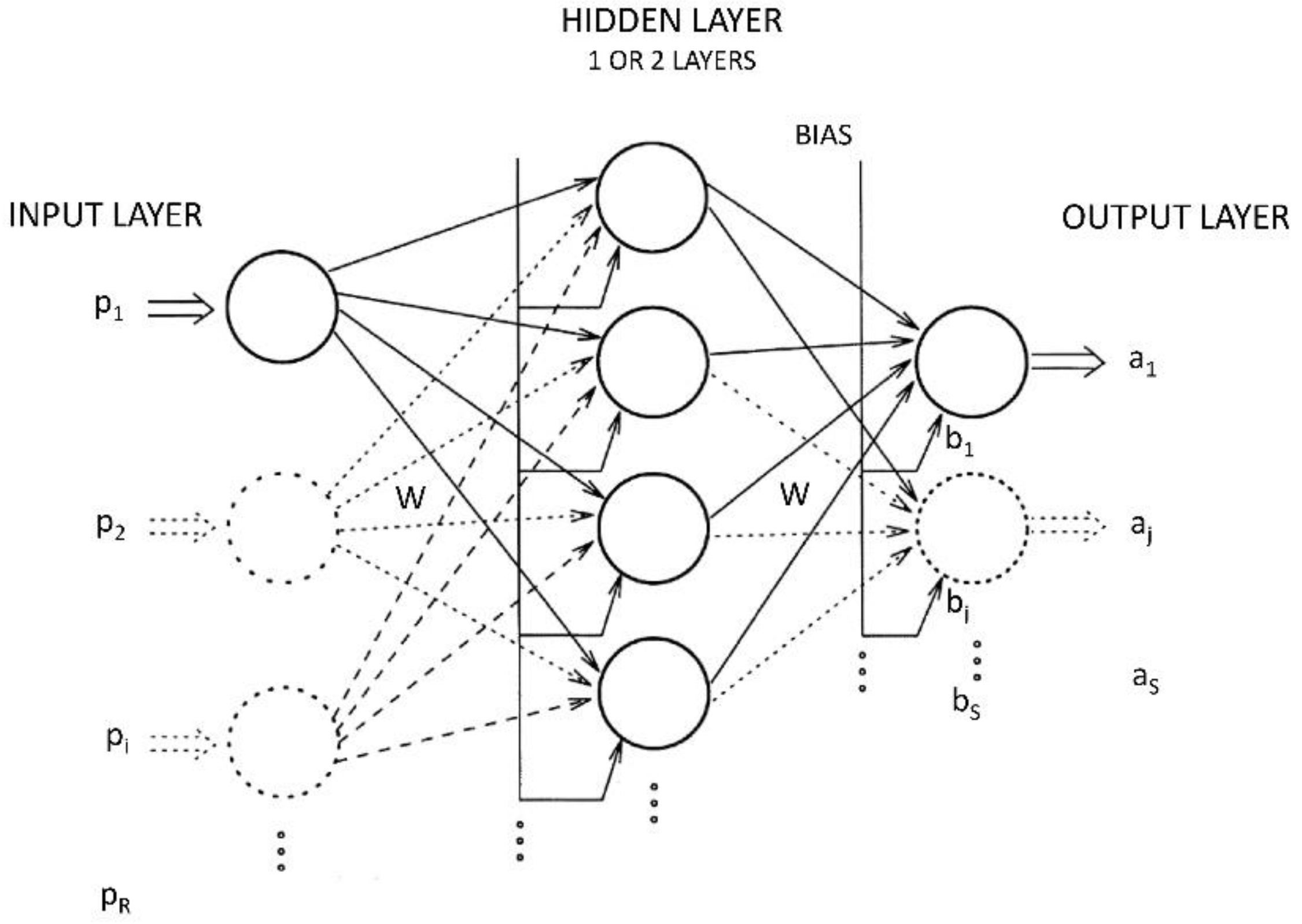
Artificial neural network (ANN) models, inspired by structure of the central nervous system, are widely used in problems of learning and pattern recognition. Here a feed forward artificial neural network (FFANN) model with backpropagation has been adopted to address the optimization problem [17,18], with a Multilayer Perceptron (MLP) structure [19], whose reference scheme is shown in the Figure 2.

In general, the network is composed of a wide number of largely interconnected processing units called neurons. They are linked through a bonding network of unidirectional communication channels. The strength of these bonds is represented by a numerical value named weight w. For each single input neuron, a transfer function f_t is defined, which transfers the scalar input p into output a through the relationship:

$${\mathrm{a}=\mathrm{f}}_{\mathrm{t}}\left(\mathrm{n}\right){=\mathrm{f}}_{\mathrm{t}}\left(\mathrm{w}·\mathrm{p}+\mathrm{b}\right)$$

(13)

where n is the net input, obtained by adding bias b to the product between the weight w and the scalar input p. Each layer of the neural network is then defined by:

• The input and output vectors p = (p₁, p₂, …, p_i, …, p_R) and a = (a₁, a₂, …, a_j, …, a_S), respectively;
• The weights matrix W = [w_ij], where I = 1, 2, …, R, and j = 1, 2, …, S;
• The biases vector b = (b₁, b₂, …, b_j, …, b_S).

The output of each neuron of the network is a scalar a_j (j = 1, 2, …, S), which can be generated by means of any differentiable transfer function f_t. Sigmoidal functions are widely used in fitting problems through ANN applications. Generally, a feed forward ANN contains, in addition to the input layer, at least two other layers:

• A hidden layer, with either Tansig or Logsig transfer function;
• An output layer with linear transfer function.

A feed forward ANN with backpropagation of error can potentially learn any type of input–output relationship. In order for the training to give accurate results, the more complex is the system to be interpolated, the more numerous and reliable training, test, and validation data should be, in order to train and test the network.

Network learning, at the end of training phase, remains stored in weight’s matrix W. Each neuron has a threshold of activation, related to the sum of inputs received by the network through weighed connections. Here the model is trained in such a way that a given input has to predict an output obtained by means of the stress analysis results obtained by the FEA software.

The first step in solving a fitting problem through ANN model is randomization of input data to be computed by the network. Preprocessing phase is followed by design of network’s structure. Since there is no rule of thumb to the choice of network’s architecture, it was decided to proceed with the development of different configurations, to the end of ranking their performance through the least mean square error (MSE). Five feed forward ANN, with 1 or 2 hidden layers, were implemented by MATLAB R2020a (The MathWorks Inc., Natick, MA, USA). Automatic adaptation of hyperparameters was adopted, by using the standard MATLAB routine. The characteristics of the five neural networks are described in

Table 3. Neural networks characteristics and performance results.

ID	N° Hidden Layers	Hidden Layer Transf Function	Output Layer Transf Function	N° Neurons Hidden Layers	MSE on Training Set
NN1	2	Logsig	Pure linear	20	1.47·10−5
NN2	1	Tansig	-	15	4.74·10−1
NN3	2	Logsig	Pure linear	25	4.68·10−1
NN4	2	Logsig	Pure linear	30	4.14·10−1
NN5	1	Logsig	-	35	4.67·10−1

.

The main architecture’s parameters are the type of hidden layer’s transfer function, and the number of neurons contained in the hidden layer. The latter must be equipped with great accuracy to obtain an efficient fitting process: there exist an optimum number of neurons, obtained by a choice of core business between opposing needs. On the one hand the increase in the number of neurons leads to excellent learning of the training set, on the other hand entails an increasing risk of over-fitting: this term is used to represent a situation in which a network has learned to perfection the training set but it generates mediocre predictions when changes occur to known inputs. A smaller number of neurons lead to a decrease in performance within the training set, but often increase generalization capacity of the network, defined as the accuracy of response to input data that the model has never “seen” before. On the other hand, a too low number of neurons can give rise to mediocre fitting and a long training, which does not reach a performance level sufficient to meet the stop criteria.

At each iteration, the parameters are tuned according to a training algorithm, until stopping criterion is satisfied. Algorithms for training/optimization generally used can be grouped into two main types, based on methods of descent gradient, and method of Gauss–Newton. Algorithm chosen for network training is Levenberg–Marquardt, which leverages the strengths of both those categories achieving good results for non-linear function’s fitting applications. Learning function used is gradient descendent type, with momentum weight and biases, which allows calculating variations of in weight matrix dW as a function of input matrix, and the difference between network’s responses and target simulated values. Cost function used to evaluate network’s performance is the mean square error (MSE) between forecasted response generated by the network and sample data simulated by FEA software.

After splitting sample data into three sets randomly extracted from initial sample of simulated data (Training set = 70% of samples; Validation set = 20% of samples; Test set = 10% of samples), Levenberg–Marquardt’s algorithm parameters have been set in such a way to ensure good stop criteria, in order to prevent the risk of overfitting.

Network’s training terminates when one of the stop criteria is satisfied:

• Maximum number of cycles (epochs) reached;
• Minimum gradient reached (in an iteration of a gradient descent algorithm, it is the minimum cost function’s decrease resulting by a shift of the weight vector dW; if there is no movement capable of producing a gradient higher than the minimum, the stopping criterion is satisfied and the algorithm stops);
• Maximum number of increments in validation phase is reached.

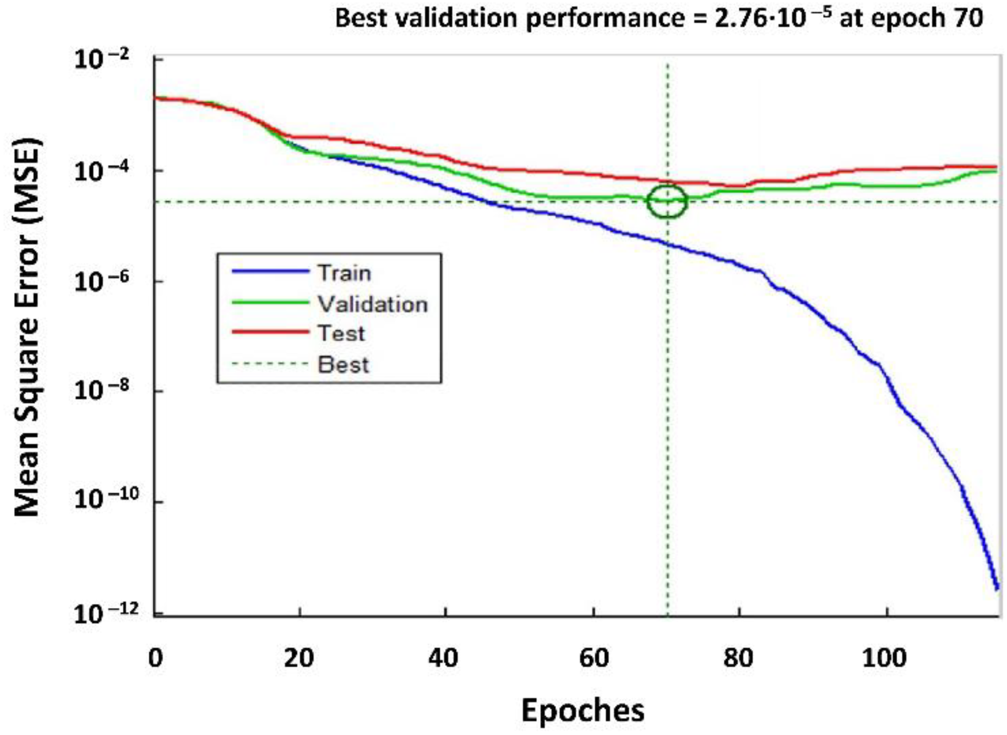
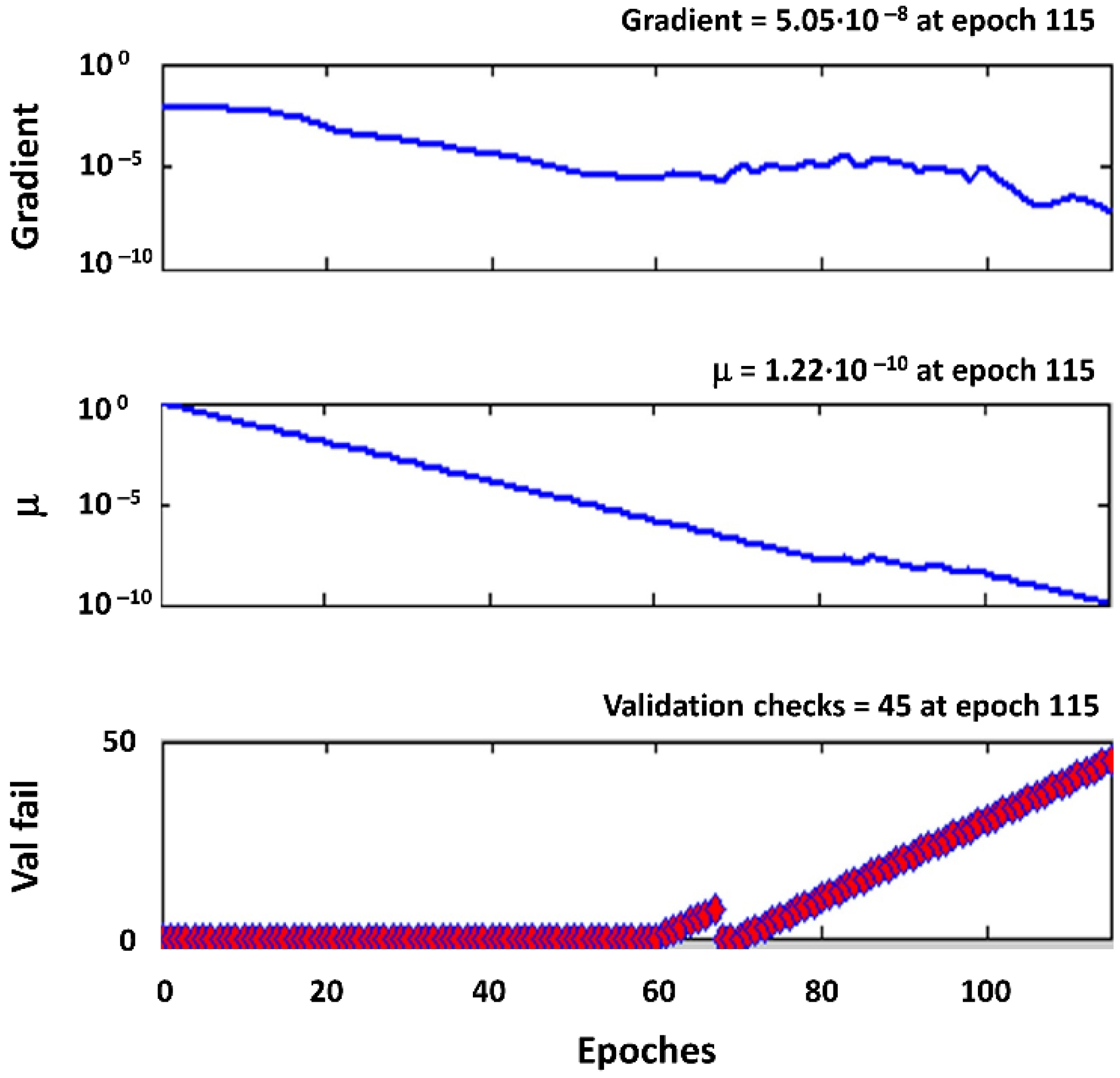
After 115 iterations of the Levenberg–Marquardt’s algorithm the training stopped and the weight matrix W was determined. Figure 3 shows the performance evaluation of training process and the performance function’s trend during the stages of training, validation and test. The values of weights w_ij stored inside matrix W, are those in correspondence of which validation error reaches a minimum, which is 2.76·10⁻⁵ at epoch 70. The trends of gradient, parameter μ (that is the NN hyperparameter used to avoid local minima in weights optimization), and validation fail are shown in Figure 4.

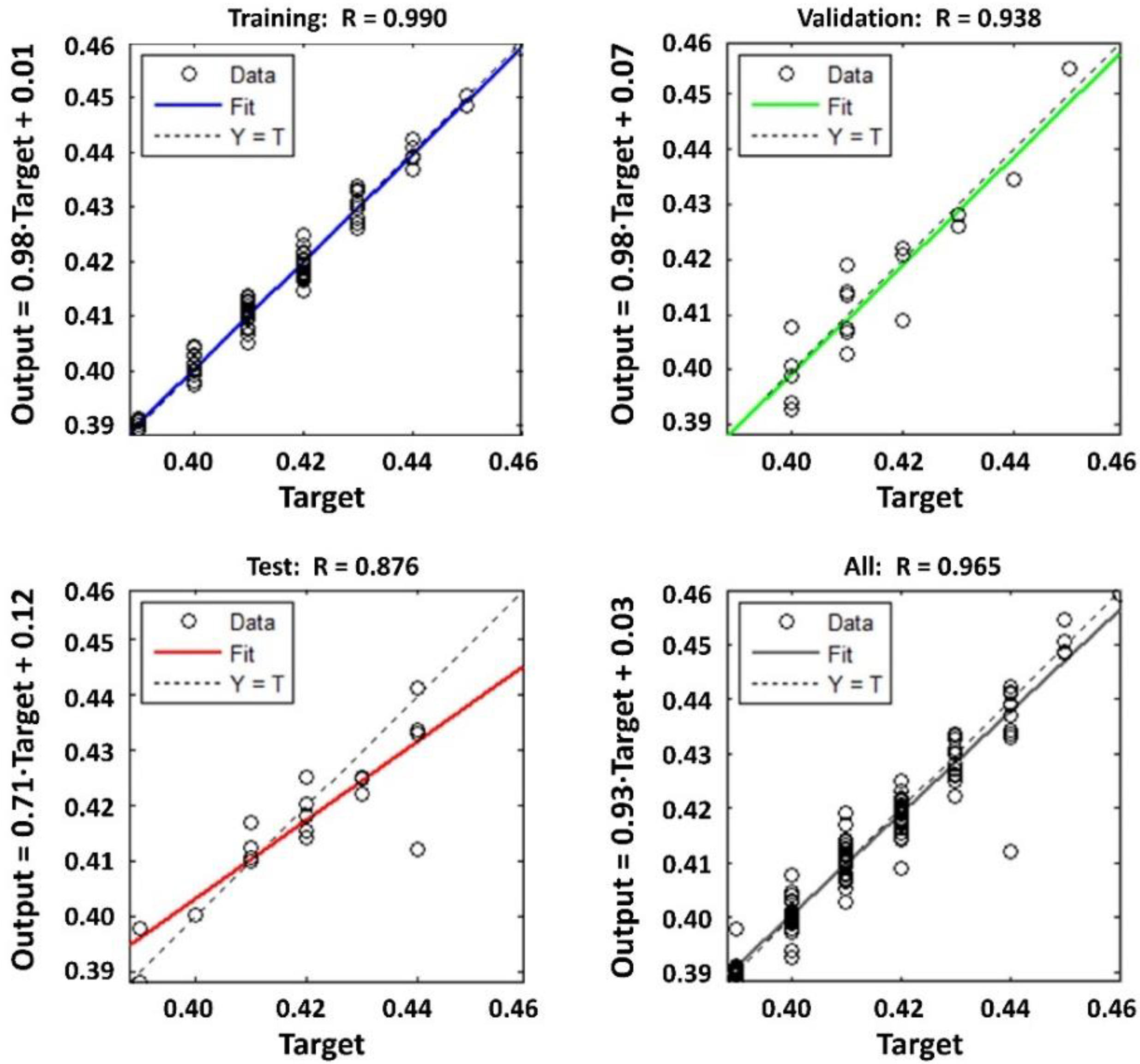
In Figure 5 the experimental observations are collocated on two axis plots. Target values are reported on abscissa, while values obtained from network’s prediction in correspondence of the same input value are reported on ordinate. In this way overfitting appears visually obvious when the points are distributed in correspondence with the bisector. The plots provide valuable information, such as performance of the fitting process respectively in the early stages of training, validation, testing, and total (overall), and the values of regressors and correlation ratio R.

3. Application and Discussion of Results

Going through the training process for the five networks configuration listed on Table 3, the results are reported in the last column, by comparison with the simulated FEA data, using MSE as performance function.

Network NN1, characterized by a MSE value that is four orders of magnitude lower than other architectures, certainly guarantees an excellent performance within the training set. Per contra, this could warned as a possible danger of overfitting, so the behavior of the network NN1 must be evaluated outside the training set. To that end, two tests are randomly selected in the training set, and a neighborhood is built around each one of them. First, a variation of each geometric loop’s parameter is generated in a range of (l, w, t) enclosed within the boundaries of the 5³ factorial domain, where the trained networks are supposed to demonstrate good prediction capacity. Geometries number o₁, …, o₈ represented in

Table 4. Tests for generalization capacity of the neural network.

ID	Variation Type	Rexp NN1	Rexp NN2	Rexp NN3
	Factorial test N° 99	6530	8900	19.05
o1	15.88 < t < 20.62	6530	8900	18.26
o2	8500 < w < 8900	6530	8850	19.05
o3	5930 < l < 6730	6630	8900	19.05
o4	Overall	6630	8850	18.26
	Factorial test N° 10	6130	8500	15.88
o5	15.88 < t < 20.62	6130	8500	16.00
o6	8500 < w < 8900	6130	8550	15.88
o7	5930 < l < 6730	6230	8500	15.88
o8	Overall	6230	8550	16.00
o9	t < 15.88	6530	8900	10.00
o10	w < 8500	6530	5000	19.05
o11	l > 6730	8000	8900	19.05
o12	Overall	8000	5000	10.00

are obtained starting from simulations N° 99 and N° 10, randomly selected from the sample of the 125 geometries simulated by the means of FEA software. Geometries number o₉, …, o₁₂ are built by varying loop’s parameters outside of factorial domain, with the aim of testing network’s performance outside the domain. Bold cells highlight the values of (l, w, t) that the neural network “does not know”.

The simulated responses obtained by the FEA for geometries o₁–o₁₂ have been compared to the ANN model predictions with the aim of evaluating generalization performance of the networks, as shown in

Table 5. Neural network generalization performance compared to FEA results.

ID	Rexp FEA	Rexp NN1	Rexp NN2	Rexp NN3	Rexp NN4	Rexp NN5
o1	0.28	0.52	0.36	0.30	0.24	0.16
o2	0.29	0.21	0.27	0.22	0.17	0.11
o3	0.28	0.16	0.23	0.18	0.25	0.26
o4	0.28	0.61	0.47	0.42	0.32	0.58
o5	0.30	0.73	0.73	0.75	0.71	0.65
o6	0.30	0.83	0.82	0.90	0.75	0.50
o7	0.30	0.53	0.58	0.67	0.66	0.58
o8	0.30	0.61	0.67	0.79	0.65	0.58
o9	0.39	0.75	0.74	0.76	0.73	0.48
o10	0.30	0.66	0.24	0.57	0.42	0.06
o11	0.51	0.77	0.19	0.95	0.27	0.08
o12	0.27	0.49	0.85	0.83	0.90	0.00

.

The outputs of the ranking process are shown in

Table 6. Neural network ranking results.

ID	MSE on Training Set	MSE Overall o1–o12	MSE within Factorial Domain o1–o8	MSE Outside of Factorial Domain o9–o12
NN1	1.47·10−5	0.10	0.10	0.09
NN2	4.74·10−1	0.22	0.09	0.55
NN3	4.68·10−1	0.15	0.12	0.22
NN4	4.14·10−1	0.10	0.08	0.14
NN5	4.67·10−1	0.08	0.06	0.16

. The networks NN1, …, NN5 have been tuned offline to predict the expansion stress ratio R_exp in response to the change of the loops geometries. The variances between the foreseen values of R_exp and the FEA data, expressed by MSE, are reported. They have been respectively calculated:

• Within the training set;
• Overall (inside and outside the domain);
• Comparing them with unknown values within the range defined by the factorial design 5³;
• Comparing them with the values outside the range defined by the factorial design 5³.

It is relevant to notice that NN1 shows the best fitting of training set, while performing well also out of the space of solutions. However, network’s configuration endowed with greater ability of generalization (i.e., more capabilities to fit experimental data) is NN5, which presents:

• The best performance interpolating factorial points characterized by MSE = 0.06;
• The minimum value of MSE inside and outside the factorial domain (0.08);
• Good knowledge of the training set, with MSE = 0.467;
• High prediction capacity in response to new inputs, expressed by the low value of MSE outside of the factorial domain (0.16), second only to the corresponding performance of NN4.

For all these reasons, NN5 can be considered as the best configuration, and adopted to continue the experiment. In order to find the optimal expansion loop geometry, the reticulum of triads (l, w, t) has been tightened increasing the number of intermediate points with a constant pitch, within the borders of the 5³ factorial design. By fragmenting into forty values each segment, initially divided into five values, a full factorial plane 40³ containing 64,000 nodes is obtained. This new reticule approximates with sufficient precision a continuum of space (l, w, t) bounded by the edges:

• 5930 ≤ l ≤ 6730
• 8500 ≤ w ≤ 8900
• 15.88 ≤ t ≤ 20.62

After having generated the plan 40³, the R_exp predicted values employing the NN5 network are reported in

Table 7. Optimization of loop’s geometry.

ID	l [mm]	w [mm]	t [mm]	Predicted Rexp
1	5990	8850	16.00	0.57
2	6270	8730	16.12	0.43
3	6370	8840	16.36	0.42
4	6510	8650	16.12	0.81
5	6490	8680	17.08	0.41
6	6050	8500	16.60	0.84
7	6410	8830	16.60	0.34
8	6370	8860	16.96	0.31
9	6230	8690	16.24	0.51
10	6730	8900	15.88	0.11
…	…	…	…	…
64000	6650	8900	19.96	0.03

.

Over the admissible region researched, the best feasible solution to the problem expressed by Equation (12) is given by the vector of variables N° 39051, reported in

Table 8. Loops optimal geometry and performances (NN predicted and FEA simulated).

ID	lopt [mm]	wopt [mm]	topt [mm]	Rexp (Tdes) NN	Rsust NN	Rexp (Tdes) FEA	Rsust FEA
39051	6730	8520	20.68	<10%	52.2%	28.2%	55.0%

with the comparison between NN predicted and FEA simulated stress ratios. It is characterized by a minimum stress ratio R_exp simulated by the network lower than 10%, and a R_sust value just above 50%, which does not compromise pipeline’s resistance to its own weight.

Although the neural network has not provided the exact value simulated by the FEA software for the optimal geometry, it has undoubtedly found a direction of minimum gradient, allowing to find an efficient set of values for (l, w, t). In fact, it optimizes the expansion stress distribution over the pipeline simulated by FEA much better than the minimum value obtained in 125 trials that make up the 5³ factorial design (R_exp = 38.7%, from Table 2). The reduction of the expansion stress ratio is equal to ΔR_exp = 38.7% − 28.2% = 10.5%.

After finding the geometry that minimizes R_exp (T_des), pipe routing was revamped by redesigning expansion loops with optimal values of the vector (l, w, t) = (l_opt, w_opt, t_opt). As overall result, simulation by means of FE model of the routing obtained by this way shows that the number of expansion loops can be halved (one loop belonging to the segment AB plus five loops belonging to BC could be removed, as highlighted by arrows in Figure 1b), keeping code stress within the allowable range by convenient margin (stress ratio 69.4%, sufficiently below the maximum limits generally imposed in the case of oil and gas process lines, up to 80%). This confirms the validity of the experimental results acknowledged.

The substantial simplification of the line obtained through optimization translates into significant lifecycle cost savings, concerning fabrication, piping installation and erection, maintenance, and final disposal.

Fabrication cost saving can be related to the quantity of material avoided to be used. The drastic reduction of the number of expansion loops obtained as a final result of the optimization, allows to replace the six loops eliminated by means of the corresponding straight section of length equal to l_opt. Neglecting the length of the six elbows for each loop (i.e., making a conservative estimate), and introducing nl_o as the number of expansion loops in the existing condition (equal to 13), and nl_opt as the number of loops in the new configuration (equal to 7), the optimization of the entire line allows saving of overall linear extension expressed by the basic efficiency metric:

$${\mathrm{SV}}_{\mathrm{LE}}={\mathrm{nl}}_{\mathrm{opt}} \left[2\left({\mathrm{w}}_{\mathrm{o}}-{\mathrm{w}}_{\mathrm{opt}}\right)+\left({\mathrm{l}}_{\mathrm{o}}-{\mathrm{l}}_{\mathrm{opt}}\right)\right]+\left({\mathrm{nl}}_{\mathrm{o}}-{\mathrm{nl}}_{\mathrm{opt}}\right) 2{\mathrm{w}}_{\mathrm{o}}$$

(14)

Using the values for w and l in the existing condition (Table 1), and after optimization (Table 8), the saving SV_LE = 98 m is obtained. Therefore, being LE_o = 415 m the extension of the existing line, and assuming the fabrication cost linearly proportional to the line extension, an approximate cost saving of 23% can be estimated.

Assessing piping installation costs in proportion to the field welding is a well-known practice. Distribution of welds between pre-fabrication and field is unpredictable at this level of analysis. However, as a first approximation can be observed that the number of welds to be executed decrease proportionally with the number of pieces in the line. The removal of 6 loops out of 13, considering 6 elbows for each loop, leads to an overall reduction in the number of elbows from 78 to 42 (46%), which involves a significant reduction in the number of welds to be made (all the more so if we consider not only the joint welds for the continuity of the line, but also those associated with supports, drains, vents, etc.).

The simplification of the line also includes beneficial effects in terms of maintenance and operation costs, which are strictly correlated with the number of components to maintain, and their linear extension.

Finally, savings in disposal cost can be estimated through the same proportion for fabrication costs. For a more accurate assessment in terms of both fabrication and disposal costs, the avoided resources consumption in terms of piping fitting cannot be neglected, as well as other savings not included in this estimate, due to reduction in piping foundations, supports, hangers, and insulation.

Another significant metric, which can quantify the efficiency of the optimization, is the weight saving, which can be estimated by:

$${\mathrm{SV}}_{\mathrm{W}}={\mathrm{LE}}_{\mathrm{o}} \mathsf{\pi } \mathrm{D} \left({\mathrm{t}}_{\mathrm{o}}-{\mathrm{t}}_{\mathrm{opt}}\right) \mathsf{\rho }+{\mathrm{SV}}_{\mathrm{LE}}{ \mathsf{\pi } \mathrm{D} \mathrm{t}}_{\mathrm{opt}} \mathsf{\rho }$$

(15)

where ρ is the density of the material. Assuming the value ρ = 7800 Kg·m³ for carbon steel, an overall savings in weight equal to 6870 Kg is calculated, which compared to the former line weight of 72,200 kg, involves a reduction of 9.5%. In this case the reduction factor is not incisive as in the case of the linear extension saving SV_LE, since the weight reduction due to the latter is compensated by the increase in the thickness of the piping due to the optimization (t_opt > t_o). Nevertheless, the weight reduction is still significant, particularly for the direct effect on metrics that can be correlated linearly to the weight; this is the case with environmental impact indicators associated to the quantity by weight of the material used and processed for fabrication and disposal of equipment and structures (such as the well-known carbon footprint).

4. Conclusions

The traditional design methodology, which is in large part based on the experience of senior designers, is focused on compliance with code requirements, generally verified by well-known numerical simulation-based tools; unfortunately, is not sufficient to assure an effective design to optimize the geometric parameters and reduce the number of expansion loops in high-pressure pipeline. Besides having awareness about the importance of an approach that relies on solid theoretical foundations, the number of aspects to take into account makes it practically impossible to obtain a closed-form analytical relation between expansion loops geometry and stress distribution.

The problem, which has been overcome through the development of a feed-forward neural network and the adoption of the Levenberg–Marquardt algorithm for network training, turned out to converge quickly at the solution. The optimal geometry for expansion loops may be defined, allowing to revamp pipe routing by halving loops number and keeping code stress within the allowable limits. As particularly significant aspects of the efficiency of the line obtained through optimization, the metrics for saving factors of linear extension and weight of the system have been formulated to obtain estimates that, although approximate, may allow for the preliminary evaluations on lifecycle costs and environmental impact of line fabrication.

Being stated in generalized terms, this optimization model can be applied to any pipeline subjected to various loadcase conditions. Compared to a traditional approach to design, which has no heuristic effectiveness, as it cannot manage the complexity of the optimization problem, the proposed approach has precisely the purpose of overcoming these limitations, providing the designer with a support that exploits the capabilities of a widely used soft computing tool such as neural network.

As a last general consideration, the proposed approach to the enhancement and optimization of the resources used to build and operate one of the fundamental components of process and fluid transport systems, and the results that can be obtained in terms of solutions efficiency, are fully aligned with many of the diversified Sustainable Development Goals (SDGs) outlined by the United Nations 2030 Agenda; the latter having become the reference framework in which the strategies for the ecological transition of industrial activities and infrastructures also find their place.