Smart Blade Flutter Alleviation with Rotational Effect

Abstract

The effect of using a piezoelectric material has been shown on postponing the flutter phenomenon on a regular blade with rotational effects in this paper. The system response of a smart blade with only flapwise and edgewise plunge and rotational DOFs showed that the oscillations of the smart blade can be effectively decayed in a very short time by using efficient piezopatches in the flapwise and edgewise plunge DOFs. Furthermore, in a smart blade with five DOFs, it has been indicated having piezopatches in flapwise and edgewise plunge DOFs can defer the flutter speed by 81.41%, which is a noticeable increase in the flutter speed. Finally, by adding a piezopatch to the pitch DOF of a smart blade, it is possible to postpone the flutter speed by 155%, which is a very considerable increase.

1. Introduction

In modern blades, because of high flexibility, aeroelastic analysis is crucial. To maximize the blade aerodynamic performance, it is very important to control aeroelastic instability [1,2]. The flutter phenomenon is one significant aeroelastic analysis. Flutter can affect negatively the blade performance even it can cause to redesign the blade. In modern blades, preventing flutter is crucial due to its effect on the long-term durability of the blade structure, energy efficiency of the system, operational safety, and performance [3,4,5,6,7].

For many years, smart materials as piezoelectric materials have been used in blade structures. Piezoelectric materials can operate as actuators and/or sensors on a blade. They can perform as dampers and actuators to control the blade aeroelastic behavior. In fact, implementing piezoelectric materials can avoid redesigning the blade which can significantly delay flutter [8,9]. These materials have been implemented on an adaptive blade with active aeroelastic control [10]. They have also been used in honeycomb materials [11]. Moreover, they can be implemented as vibration damping to control a plate under forcing function and time-dependent boundary moments [12]. In addition, piezoelectric materials can perform as flutter controllers by using the finite element method in damaged composite laminates [13]. Those materials can be used to study aeroelastic flutter analysis on thick porous plates [14]. Moreover, piezoelectric actuators and sensors have been investigated in aeroelastic optimization [15]. The blade’s aeroelastic behavior can be effectively modified by implementing piezopatch including a shunt circuit. Previously, there were some practical limits in the existing low-frequency range in aeroelastic phenomena because of the large size required inductance for passive aeroelastic control. However, nowadays, having a small-size inductor combined with a piezopatch can facilitate passive aeroelastic control [16]. Practically because of having too large internal resistance, standard inductors are not appropriate to be combined with a piezopatch for resonant shunt applications. By using closed magnetic circuits with high-level-permeability materials, it is possible to design large inductance inductors which have high-quality factors.

Damping in the blade structure without causing any instability can be augmented by using shunted piezopatches. Furthermore, shunted piezopatches are simple to apply and need little to no power. Their hardware needs piezoelectrics with a simple electric circuit which includes a capacitor, an inductor, and a resistor. The shunted piezopatches consume the energy created from the blade vibrations to control the blade aeroelastic vibration, which can reduce the oscillations of specific frequencies and modes.

In this paper, the flutter speed of a simple aeroelastic system can be increased by using piezoelectric materials. One system is a 2D blade with two piezoelectric patches which had flapwise and edgewise plunge DOFs as well as rotational DOFs. Later, another system used is a 2D blade including a piezoelectric patch with plunge, pitch, and control rotational degrees of freedom (DOFs) subjected to unsteady aerodynamic loads. The work objective was to present the effect of piezoelectric patches that can influence effectively a simple smart blade system with rotational effects.

In Section 2, the smart blade equations of motion with flapwise and edgewise plunge and rotational DOFs were described to solve those equations to calculate the flapwise and edgewise plunge velocities, displacements, electrical currents, and electric charges as well as rotational velocities and displacements. Then, the system fixed points and their stability around those points were studied to present the system response. Example 1 shows the considerable decay in the vibration of a smart blade in comparison to that in the vibration of a regular blade.

Section 3 shows a smart blade with plunge, pitch, and control DOFs and two piezopatches with flapwise and edgewise plunge and rotational DOFs to obtain the equations of motion under unsteady aerodynamic loads. Solving the system of equations provides the flapwise and edgewise plunge velocities, displacements, electrical currents, and electric charges as well as the pitching velocity, rotation, electrical current, and electric charge. Afterwards, by obtaining the flutter speed, we indicated how adding two piezopatches can effectively defer the flutter.

In Section 4, a smart blade with plunge, pitch, and control DOFs and piezopatches with plunge and pitch DOFs are presented. The results showed that the flutter speed can even be further raised by having three piezopatches.

In addition, the smart blade concept presented in this work can be applied to increase the performance of renewable energy devices such as wind turbine and marine turbine blades [17,18].

2. Aeroelastic Analysis of the Smart Blade

Before investigating the aeroelastic smart blade, it requires investigating the aeroelastic stability of the smart blade. The time response of the aeroelastic system can be written as [19]:

$$x\left(t\right)={{\displaystyle \sum }}_{i=1}^n{v}_i{e}^{{\lambda }_{i}t}{b}_i,$$

(1)

where $v_i$ is the smart blade spatial deformation, $e^{{\lambda }_{i}t}$ is the smart blade temporal deformation, and $b_i$ is the eigenvector. It is a good idea to study the fixed-point characteristics of three smart blades with DOFs in flapwise and edgewise plunge motions separately.

A Smart Blade with Only Plunge and Rotational DOFs

A smart blade which has flapwise and edgewise plunge and rotational DOFs is considered, as shown in Figure 1.

By assuming a constant rotational velocity, the smart blade equations of motion with two plunge and rotational DOFs in free vibrations can be written as below:

$$\left\{\begin{array}{l}m{\ddot{h}}_1+C_{h_1}{\dot{h}}_1+K_{h_1}{h}_1-{\beta }_{h_1}{q}_{h_1}=0\\ L_{h_1}{\ddot{q}}_{h_1}+R_{h_1}{\dot{q}}_{h_1}+\frac{1}{C_{p{h}_1}}{q}_{h_1}-{\beta }_{h_1}{h}_1=0\\ m\left({\ddot{h}}_2+r\ddot{\gamma }\right)+C_{h_2}{\widehat{h}}_2+K_{h_2}{h}_2-{\beta }_{h_2}{q}_{h_2}=0\\ L_{h_2}{\ddot{q}}_{h_2}+R_{h_2}{\dot{q}}_{h_2}+\frac{1}{C_{p{h}_2}}{q}_{h_2}-{\beta }_{h_2}{h}_2=0\\ mr\ddot{\gamma }-\frac{P}{r{\mathsf{\Omega }}^2}\dot{\gamma }-C_{h_2}{h}_2-K_{h_2}{h}_2=0\end{array}\right.$$

(2)

where the parameters can be as below:

$m$	mass of the smart blade
$C_{h_1}$	flapwise structural damping of the smart blade
$K_{h_1}$	flapwise structural stiffness
$h_1$	instantaneous flapwise displacement
${\beta }_{h_1}$	flapwise plunge electromechanical coupling
$q_{h_1}$	flapwise plunge electric charge
$L_{h_1}$	flapwise piezoelectric material plunge inductance
$R_{h_1}$	flapwise piezoelectric material plunge resistance
$C_{p{h}_1}$	flapwise plunge capacitance of the piezoelectric material
$r$	distance from the hub
$\gamma$	rotational displacement of the smart blade
$C_{h_2}$	edgewise structural damping of the smart blade
$K_{h_2}$	edgewise structural stiffness
$h_2$	instantaneous edgewise displacement
${\beta }_{h_2}$	edgewise plunge electromechanical coupling
$q_{h_2}$	edgewise plunge electric charge
$L_{h_2}$	edgewise piezoelectric material plunge inductance
$R_{h_2}$	edgewise piezoelectric material plunge resistance
$C_{p{h}_2}$	edgewise plunge capacitance of the piezoelectric material
$P$	hub force
$\mathsf{\Omega }$	rotational speed of the smart blade

As explained before, the flapwise plunge electromechanical coupling may be calculated as ${\beta }_{h_1}=e_{h_1}/C_{p{h}_1},$ where $e_{h_1}$ is the flapwise plunge coupling coefficient, and the edgewise plunge electromechanical coupling may be calculated as ${\beta }_{h_2}=e_{h_2}/C_{p{h}_2},$ where $e_{h_2}$ is the edgewise plunge coupling coefficient. Considering $x_1={\dot{h}}_1$, $x_2=h_1$, $x_3={\dot{q}}_{h_1}$, $x_4=q_{h_1}$, $x_5={\dot{h}}_2$, $x_6=h_2$, $x_7={\dot{q}}_{h_2}$, $x_8=q_{h_2}$, $x_9=\dot{\gamma }$, and $x_{10}=\gamma$, Equation (2) may be written as first-order differential equations:

$$\left\{\begin{array}{c}{\dot{x}}_1=-\frac{C_{h_1}}{m}{x}_1-\frac{K_{h_1}}{m}{x}_2+\frac{{\beta }_{h_1}}{m}{x}_4\hfill \\ {\dot{x}}_2=x_1\hfill \\ {\dot{x}}_3=-\frac{R_{h_1}}{L_{h_1}}{x}_3-\frac{1}{C_{p{h}_1}{L}_{h_1}}{x}_4+\frac{{\beta }_{h_1}}{L_{h_1}}{x}_1\hfill \\ {\dot{x}}_4=x_3\hfill \\ {\dot{x}}_5+r{\dot{x}}_9=-\frac{C_{h_2}}{m}{x}_5-\frac{K_{h_2}}{m}{x}_6+\frac{{\beta }_{h_2}}{m}{x}_8.\hfill \\ {\dot{x}}_6=x_5\hfill \\ {\dot{x}}_7=-\frac{R_{h_2}}{L_{h_2}}{x}_7-\frac{1}{C_{p{h}_2}{L}_{h_2}}{x}_8+\frac{{\beta }_{h_2}}{L_{h_2}}{x}_6\hfill \\ {\dot{x}}_8=x_7\hfill \\ {\dot{x}}_9=\frac{P}{m{r}^2{\mathsf{\Omega }}^2}{x}_5+\frac{C_{h_2}}{mr}{x}_5+\frac{K_{h_2}}{mr}{x}_6\hfill \\ {\dot{x}}_{10}=x_9\hfill \end{array}\right.$$

(3)

Defining and $\mathit{q}={[m{C}_{h_1} K_{h_1} {\beta }_{h_1} L_{h_1} R_{h_1} C_{{ph}_1} C_{h_2} K_{h_2} {\beta }_{h_2} L_{h_2} R_{h_2} C_{{ph}_2} r \Omega ]}^T$ and x = [x₁ x₂ x₃ x₄ x₅ x₆ x₇ x₈ x₉ x₁₀]^T, Equation (3) can be written as:

$$\left[\begin{array}{cccccccccc}1\hfill & 0\hfill & 0\hfill & 0\hfill & 0\hfill & 0\hfill & 0\hfill & 0\hfill & 0\hfill & 0\hfill \\ 0\hfill & 1\hfill & 0\hfill & 0\hfill & 0\hfill & 0\hfill & 0\hfill & 0\hfill & 0\hfill & 0\hfill \\ 0\hfill & 0\hfill & 1\hfill & 0\hfill & 0\hfill & 0\hfill & 0\hfill & 0\hfill & 0\hfill & 0\hfill \\ 0\hfill & 0\hfill & 0\hfill & 1\hfill & 0\hfill & 0\hfill & 0\hfill & 0\hfill & 0\hfill & 0\hfill \\ 0\hfill & 0\hfill & 0\hfill & 0\hfill & 1\hfill & 0\hfill & 0\hfill & 0\hfill & r\hfill & 0\hfill \\ 0\hfill & 0\hfill & 0\hfill & 0\hfill & 0\hfill & 1\hfill & 0\hfill & 0\hfill & 0\hfill & 0\hfill \\ 0\hfill & 0\hfill & 0\hfill & 0\hfill & 0\hfill & 0\hfill & 1\hfill & 0\hfill & 0\hfill & 0\hfill \\ 0\hfill & 0\hfill & 0\hfill & 0\hfill & 0\hfill & 0\hfill & 0\hfill & 1\hfill & 0\hfill & 0\hfill \\ 0\hfill & 0\hfill & 0\hfill & 0\hfill & 0\hfill & 0\hfill & 0\hfill & 0\hfill & 1\hfill & 0\hfill \\ 0\hfill & 0\hfill & 0\hfill & 0\hfill & 0\hfill & 0\hfill & 0\hfill & 0\hfill & 0\hfill & 1\hfill \end{array}\right]\dot{\mathbf{x}}=\mathbf{f}(\mathbf{x},\mathit{q})=\left[\begin{array}{c}-\frac{C_{h_1}}{m}{x}_1-\frac{K_{h_1}}{m}{x}_2+\frac{{\beta }_{h_1}}{m}{x}_4\\ x_1\\ -\frac{R_{h_1}}{L_{h_1}}{x}_3-\frac{1}{C_{p{h}_1}{L}_{h_1}}{x}_4+\frac{{\beta }_{h_1}}{L_{h_1}}{x}_2\\ x_3\\ -\frac{c_{h_2}}{m}{x}_5-\frac{K_{h_2}}{m}{x}_6+\frac{{\beta }_{h_2}}{m}{x}_8\\ x_5\\ -\frac{R_{h_2}}{L_{h_2}}{x}_7-\frac{1}{c_{p{h}_2}{L}_{h_2}}{x}_8+\frac{{\beta }_{h_2}}{L_{h_2}}{x}_6\\ x_7\\ \frac{P}{m{r}_7{\mathsf{\Omega }}^2}{x}_5+\frac{c_{h_2}}{mr}{x}_5+\frac{K_{h_2}}{mr}{x}_6\\ x_9\end{array}\right]$$

(4)

where $f$ presents linear functions, and $x_1$, $x_2$, $x_3$, $x_4$, $x_5$, $x_6$, $x_7$, $x_8$, $x_9$, and $x_{10}$ are the smart blade states and represent the system’s flapwise velocity, flapwise displacement, flapwise electrical current, flapwise electric charge response, edgewise velocity, edgewise displacement, edgewise electrical current, edgewise electric charge response, angular velocity, and angular displacement, respectively. The three aeroelastic smart blade system with DOFs had 10 eigenvalues that explained the fixed point stability. The static solutions or fixed points of the system are calculated from the following solutions:

$$f\left(x,\mathit{q}\right)=\mathbf{0},$$

(5)

or equivalently,

$$\dot{x}=\mathbf{0}.$$

(6)

By considering Equations (4) and (6), the following equations can be presented as:

$$\mathit{B}\dot{x}=\mathit{A}\left(\mathit{q}\right)x,$$

(7)

or

$$\dot{x}={\mathit{B}}^{-1}\mathit{A}\left(\mathit{q}\right)x,$$

(8)

where

$$\mathit{B}=\left[\begin{array}{cccccccccc}1\hfill & 0\hfill & 0\hfill & 0\hfill & 0\hfill & 0\hfill & 0\hfill & 0\hfill & 0\hfill & 0\hfill \\ 0\hfill & 1\hfill & 0\hfill & 0\hfill & 0\hfill & 0\hfill & 0\hfill & 0\hfill & 0\hfill & 0\hfill \\ 0\hfill & 0\hfill & 1\hfill & 0\hfill & 0\hfill & 0\hfill & 0\hfill & 0\hfill & 0\hfill & 0\hfill \\ 0\hfill & 0\hfill & 0\hfill & 1\hfill & 0\hfill & 0\hfill & 0\hfill & 0\hfill & 0\hfill & 0\hfill \\ 0\hfill & 0\hfill & 0\hfill & 0\hfill & 1\hfill & 0\hfill & 0\hfill & 0\hfill & r\hfill & 0\hfill \\ 0\hfill & 0\hfill & 0\hfill & 0\hfill & 0\hfill & 1\hfill & 0\hfill & 0\hfill & 0\hfill & 0\hfill \\ 0\hfill & 0\hfill & 0\hfill & 0\hfill & 0\hfill & 0\hfill & 1\hfill & 0\hfill & 0\hfill & 0\hfill \\ 0\hfill & 0\hfill & 0\hfill & 0\hfill & 0\hfill & 0\hfill & 0\hfill & 1\hfill & 0\hfill & 0\hfill \\ 0\hfill & 0\hfill & 0\hfill & 0\hfill & 0\hfill & 0\hfill & 0\hfill & 0\hfill & 1\hfill & 0\hfill \\ 0\hfill & 0\hfill & 0\hfill & 0\hfill & 0\hfill & 0\hfill & 0\hfill & 0\hfill & 0\hfill & 1\hfill \end{array}\right]$$

(9)

$$\mathit{A}=\left[\begin{array}{cccccccccc}-\frac{c_{h_1}}{m}& -\frac{K_{h_1}}{m}& 0& \frac{{\beta }_{h_1}}{m}& 0& 0& 0& 0& 0& 0\\ 1& 0& 0& 0& 0& 0& 0& 0& 0& 0\\ 0& \frac{{\beta }_{h_1}}{L_{h_1}}& -\frac{R_{h_1}}{L_{h_1}}& -\frac{1}{C_{p{h}_1}{L}_{h_1}}& 0& 0& 0& 0& 0& 0\\ 0& 0& 1& 0& 0& 0& 0& 0& 0& 0\\ 0& 0& 0& 0& -\frac{c_{h_2}}{m}& -\frac{K_{h_2}}{m}& 0& \frac{{\beta }_{h_2}}{m}& 0& 0\\ 0& 0& 0& 0& 1& 0& 0& 0& 0& 0\\ 0& 0& 0& 0& 0& \frac{{\beta }_{h_2}}{L_{h_2}}& -\frac{R_{h_2}}{L_{h_2}}& -\frac{1}{C_{p{h}_2}{L}_{h_2}}& 0& 0\\ 0& 0& 0& 0& 0& 0& 1& 0& 0& 0\\ 0& 0& 0& 0& \frac{P}{m{r}^2{\mathsf{\Omega }}^2}+\frac{C_{h_2}}{mr}& \frac{K_{h_2}}{mr}& 0& 0& 0& 0\\ 0& 0& 0& 0& 0& 0& 0& 0& 1& 0\end{array}\right]$$

(10)

The solution of Equation (8) can be written as Equation (1), where $v_i$ is the ith eigenvector of ${\mathit{B}}^{-1}\mathit{A}$, ${\lambda }_i$ is the ith eigenvalue of ${\mathit{B}}^{-1}\mathit{A}$, and $b_i$ is the ith element of $\mathit{b}={\mathit{V}}^{-1}{x}_0$, where $\mathit{V}$ is the eigenvector of ${\mathit{B}}^{-1}\mathit{A}$ and ${\mathbf{x}}_0$ is the initial condition.

Example 1.

A smart blade with flapwise and edgewise plunge and rotational DOFs in the system response.

In the first example, a smart blade with only flapwise and edgewise plunge and rotational DOFs (Figure 1) is considered, which has the following characteristics as [8]:

$m=0.3872 \mathrm{Kg}$	$C_{h_1}=0.3237 \mathrm{Ns}/\mathrm{m}$
$K_{h_1}=13380 \mathrm{N}/\mathrm{m}$	$e_{h_1}=80\times {10}^{-3} \mathrm{C}/\mathrm{m}$
$C_{p{h}_1}=1680 \mathrm{nF}$	$L_{h_1}=0.1 \mathrm{H}$
$R_{h_1}=4050 \mathsf{\Omega }$	$C_{h_2}=0.5 \mathrm{Ns}/\mathrm{m}$
$K_{h_2}=32112 \mathrm{N}/\mathrm{m}$	$e_{h_2}=7.55\times {10}^{-2} \mathrm{C}/\mathrm{m}$
$C_{p{h}_2}=268 \mathrm{nF}$	$L_{h_2}=0.1 \mathrm{H}$
$R_{h_2}=9050 \mathsf{\Omega }$	$P=1 \mathrm{N}$
$r=1 \mathrm{m}$	$\mathsf{\Omega }=10 \mathrm{rad}/\mathrm{s}$

and the initial conditions are as follows:

x1(0) = 0.1 m/s	x2(0) = 0 m
x3(0) = 0 A	x4(0) = 0 C
x5(0) = 0.1 m/s	x6(0) = 0 m
x7(0) = 0 A	x8(0) = 0 C
x9(0) = 0.1 rad/s	x10(0) = 0 rad

Figure 2 depicts the system response of velocity. The solid line represents the velocity of the smart blade, and the dashed line shows the velocity of the regular blade. As indicated in Figure 2, the vibrations can very effectively decay by the piezoelectric patches. Both system responses oscillate by decaying their amplitudes with time towards zero, which are called as damped responses. From Figure 2, it is clear that the amplitude of the smart blade responses can decay much faster than the one of the regular blade responses. The flapwise oscillation of the smart blade (Figure 2a) decays for almost $0.4 \mathrm{s};$ however, the flapwise oscillation of the regular blade takes around $12 \mathrm{s}$ to decay. Moreover, the edgewise oscillation of the smart blade (Figure 2b) decays $0.2 \mathrm{s};$ however, the edgewise oscillation of the regular blade takes around $8 \mathrm{s}$ to decay.

Figure 3 depicts the system response of displacement. The solid line represents the displacement of the smart blade, and the dashed line shows the displacement of the regular blade. As indicated in Figure 3, the vibrations can very effectively decay by the piezoelectric patches. Both system responses oscillate by decaying their amplitudes with time towards zero, which are called as damped responses. From Figure 3, it is clear that the amplitude of the smart blade responses can decay much faster than the one of the regular blade responses. The flapwise oscillation of the smart blade (Figure 3a) decays for almost $0.4 \mathrm{s}$; however, the flapwise oscillation of the regular blade takes around $12 \mathrm{s}$ to decay. Moreover, the edgewise oscillation of the smart blade (Figure 3b) decays for $0.2 \mathrm{s}$; however, the edgewise oscillation of the regular blade takes around $10 \mathrm{s}$ to decay.

Furthermore, the velocities and the displacements phase plane plots depict the point (0,0) recalls the system trajectory, as shown in Figure 4. The flapwise and edgewise trajectories of the smart blade start from the initial displacements and velocities at the far top, and it turns to the center of the phase plane, where (0,0) is the fixed point and x_F = 0. In fact, the phase plane plots indicate that the fixed points draw the smart blade trajectories.

Likewise, the electrical current and the charge phase plane start at the electrical current and charge initial conditions which are zeros, and they turn out counter-clockwise until arriving at the maximum values. The trajectories then turn towards the start point $\left(0,0\right)$, as shown in Figure 5.

Figure 6 depicts the system response of the rotational velocity. The solid line represents the rotational velocity of the smart blade, and the dashed line shows the rotational velocity of the regular blade. As indicated in Figure 6, the vibrations can very effectively decay by the piezoelectric patches. Both system responses oscillate by decaying their amplitudes with time towards zero, which are called as damped responses. From Figure 6a, it is clear that the amplitude of the smart blade responses can decay much faster than the amplitude of the regular blade responses. The oscillation of the rotational velocity of the smart blade decays for almost $0.15 \mathrm{s};$ however, the oscillation of the rotational velocity of the regular blade takes around $5 \mathrm{s}$ to decay, and it increases in the equilibrium position, as indicated in Figure 6b.

Figure 7 depicts the system response of the rotational displacement. The solid line represents the rotational displacement of the smart blade, and the dashed line shows the rotational displacement of the regular blade. As indicated in Figure 7, the vibrations can very effectively decay by the piezoelectric patches. Both system responses oscillate by decaying their amplitudes with time towards zero, which are called as damped responses. From Figure 7, it is clear that the amplitude of the smart blade responses decays much faster than the amplitude of the regular blade responses. The oscillation of the rotational displacement of the smart blade (Figure 7b) decays for almost $0.2 \mathrm{s};$ however, the oscillation of the rotational displacement of the regular blade takes around $1 \mathrm{s}$ to decay.

However, by considering $P=0$ in Equation (2), the system response of the rotational displacement can be changed as indicated in Figure 8, in which the mean value of the rotational displacement of the regular blade is not increased with the increase in time.

3. Smart Blade with Plunge, Pitch, and Control DOFs and Piezopatches with Plunge DOFs

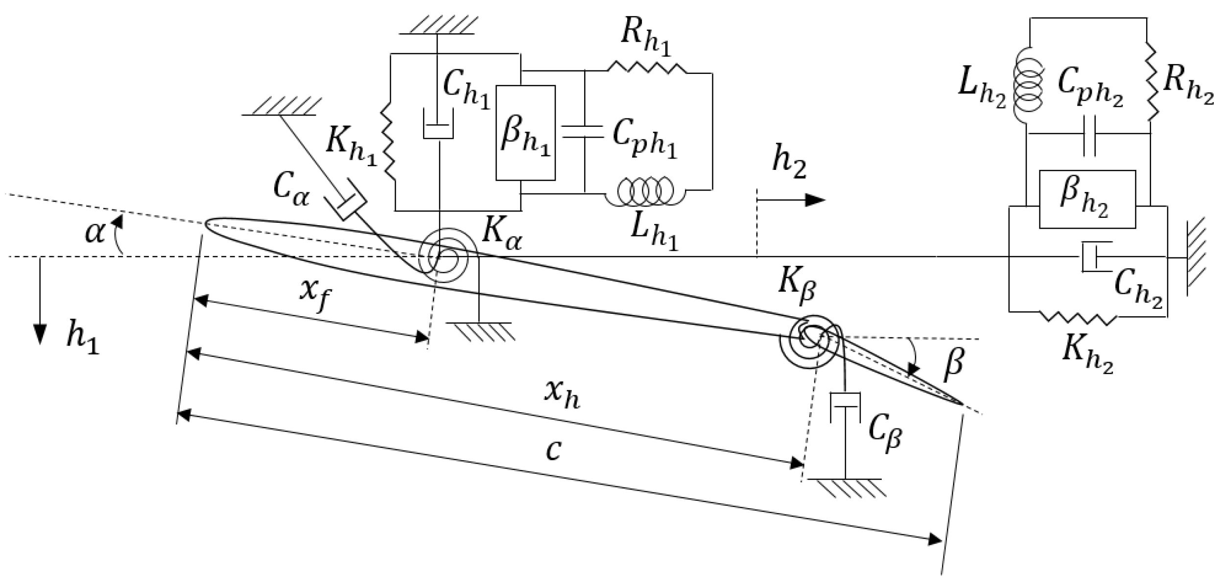
Figure 9 depicts a 2D smart blade with plunge, pitch, and control degrees of freedom. In the model, there are an airfoil with two piezoelectric patches in the flapwise and edgewise plunge DOFs. The system includes flapwise and edgewise plunge, pitch, and control degrees of freedom (DOFs) indicated by $h_1$, $h_2$, $\alpha$, and $\beta$, respectively. The control surface angle around its hinge, located at distance $x_h$ from the leading edge, is represented by the DOF $\beta ,$ and the stiffness of the control surface is denoted by $K_{\beta }$.

Using the Lagrange’s equations and the Kirchhoff’s law leads to the equations of motion as:

$$\left\{\begin{array}{c}m{\ddot{h}}_1+S_{\alpha h}\ddot{\alpha }+S_{\beta }\ddot{\beta }+C_{h_1}{\dot{h}}_1+K_{h_1}{h}_1-{\beta }_{h_1}{q}_{h_1}=-L\hfill \\ S_{\alpha h}{\ddot{h}}_1+I_{\alpha }\ddot{\alpha }+I_{\alpha \beta }\ddot{\beta }+C_{\alpha }\dot{\alpha }+K_{\alpha }\alpha =M_{xf}\hfill \\ S_{\beta }{\ddot{h}}_1+I_{\alpha \beta }\ddot{\alpha }+I_{\beta }\ddot{\beta }+C_{\beta }\dot{\beta }+K_{\beta }\beta =M_{xh}\hfill \\ L_{h_1}{\ddot{q}}_{h_1}+R_{h_1}{\dot{q}}_{h_1}+\frac{1}{C_{p{h}_1}}{q}_{h_1}-{\beta }_{h_1}{h}_1=0\hfill \\ m\left({\ddot{h}}_2+r\ddot{\gamma }\right)+C_{h_2}{\dot{h}}_2+K_{h_2}{h}_2-{\beta }_{h_2}{q}_{h_2}=0\hfill \\ L_{h_2}{\ddot{q}}_{h_2}+R_{h_2}{\dot{q}}_{h_2}+\frac{1}{C_{p{h}_2}}{q}_{h_2}-{\beta }_{h_2}{h}_2=0\hfill \\ mr\ddot{\gamma }-\frac{P}{r{\mathsf{\Omega }}^2}\dot{\gamma }-C_{h_2}{\dot{h}}_2-K_{h_2}{h}_2=0\hfill \end{array}\right.$$

(11)

where $m$, $C_{h_1}$, $K_{h_1}$, $h_1$, ${\beta }_{h_1}$, $q_{h_1}$, $L_{h_1}$, $R_{h_1}$, $C_{p{h}_1}$, $C_{h_2}$, $K_{h_2}$, $h_2$, $\gamma$, ${\beta }_{h_2}$, $q_{h_2}$, $L_{h_2}$, $R_{h_2}$, $C_{p{h}_2}$, $P$, $r$, and $\mathsf{\Omega }$ are defined as in Equation (2) and the rest are as follows:

$S_{\alpha h}$	static mass moment of the blade around the pitch axis $x_f$
$S_{\beta }$	static mass moment of the control surface around the hinge axis $x_h$
$I_{\beta }$	control surface moment of the inertia around the hinge axis
$I_{\alpha \beta }$	Product of the inertia of the blade and the control surface
$L$	lift
$M_{xf}$	pitching moment of the blade around the pitch axis $x_f$
$M_{xh}$	pitching moment of the control surface around the hinge axis $x_h$

By having unsteady aerodynamics, the lift and moments can be given as follows [17,18]:

$$\begin{gathered} L\left(t\right)=\rho b^2\left(U\pi \dot{\alpha }+\pi \ddot{h}-\pi ba\ddot{\alpha }-U{T}_4\dot{\beta }-T_{1}b\ddot{\beta }\right) \\ +2\pi \rho bU\left(\mathsf{\Phi }\left(0\right)w-{{\displaystyle \int }}_0^t\frac{\partial \mathsf{\Phi }\left(t-t_0\right)}{\partial t_0}w\left(t_0\right)d{t}_0\right), \end{gathered}$$

(12)

$$\begin{gathered} M_{xf}=-\rho b^2\left(-a\pi b\ddot{h}+\pi b^2\left(\frac{1}{8}+a^2\right)\ddot{\alpha }-\left(T_7+\left(c_h-a\right)T_1\right)b^2\ddot{\beta }\right) \\ -\rho b^2\left(\pi \left(\frac{1}{2}-a\right)Ub\dot{\alpha }+\left(T_1-T_8-\left(c_h-a\right)T_4+\frac{T_{11}}{2}\right)Ub\dot{\beta }\right)-\rho b^2\left(T_4+T_{10}\right)U^2\beta \\ +2\rho U{b}^2\pi \left(a+\frac{1}{2}\right)\left(\mathsf{\Phi }\left(0\right)w-{{\displaystyle \int }}_0^t\frac{\partial \mathsf{\Phi }\left(t-t_0\right)}{\partial t_0}w\left(t_0\right)d{t}_0\right), \end{gathered}$$

(13)

$$\begin{gathered} M_{xh}=-\rho b^2\left(-T_{1}b\ddot{h}+2T_{13}{b}^2\ddot{\alpha }-\frac{1}{\pi }{T}_3{b}^2\ddot{\beta }\right) \\ -\rho b^2\left(\left(-2T_9-T_1+T_4\left(a-\frac{1}{2}\right)\right)Ub\dot{\alpha }-\frac{1}{2\pi }Ub{T}_4{T}_{11}\dot{\beta }\right) \\ -\frac{\rho b^2{U}^2}{\pi }\left(T_5-T_4{T}_{10}\right)\beta -\rho b^{2}U{T}_{12}\left(\mathsf{\Phi }\left(0\right)w-{{\displaystyle \int }}_0^t\frac{\partial \mathsf{\Phi }\left(t-t_0\right)}{\partial t_0}w\left(t_0\right)d{t}_0\right) . \end{gathered}$$

(14)

Substituting Equations (12)−(14) into Equation (10) provides a set of equations of motion only in the time-dependent form and can be solved numerically such as using the backward finite difference scheme in numerical integration [20]. However, the equations of motion can be given as ordinary differential equations by using the exponential form of the Wagner function’s approximation. These equations can be solved analytically rather than numerically; therefore, they would be much more practical [21,22]. The Wagner function’s approximation can be presented as:

$$\mathsf{\Phi }\left(t\right)=1-{\mathsf{\Psi }}_1{e}^{-{\epsilon }_{1}Ut/b}-{\mathsf{\Psi }}_2{e}^{-{\epsilon }_{2}Ut/b},$$

(15)

where ${\mathsf{\Psi }}_1=0.165$, ${\mathsf{\Psi }}_2=0.335$, ${\epsilon }_1=0.0455$, and ${\epsilon }_2=0.3$.

The equations of motion in the full unsteady aeroelastic form can be given as follows:

$$\begin{gathered} \left(\mathit{A}+\rho \mathit{B}\right)\ddot{\mathit{y}}+\left(\mathit{C}+\rho U\mathit{D}\right)\dot{\mathit{y}}+\left(\mathit{E}+\rho U^2\mathit{F}\right)\mathit{y}+\rho U^3\mathit{W}=\rho U\mathbf{g}\dot{\mathsf{\Phi }}\left(t\right) \\ \dot{\mathit{w}}-{\mathit{W}}_1\mathit{y}-U{\mathit{W}}_2\mathit{w}=0, \end{gathered}$$

(16)

where $\mathit{y}={\left[h_1\hspace{1em}\alpha \hspace{1em}\beta \hspace{1em}{q}_{h_1}\hspace{1em}{h}_2\hspace{1em}{q}_{h_2}\hspace{1em}\gamma \right]}^T$ represents the displacement and the charge vector, $\mathit{w}={\left[w_1\hspace{1em}\cdots \hspace{1em}{w}_6\hspace{1em}0\right]}^T$ gives the aerodynamic states vector, $\mathsf{\Phi }\left(t\right)$ presents the Wagner function, $\mathit{A}$ is the inductance and structural mass matrix, $\mathit{B}$ represents the aerodynamic mass matrix, $\mathit{E}$ gives the structural stiffness and resistance matrix, $\mathit{F}$ is the aerodynamic stiffness matrix, $\mathit{W}$ represents the influence matrix of aerodynamic state, $\mathbf{g}$ gives the initial condition excitation vector, and ${\mathit{W}}_1$ and ${\mathit{W}}_2$ present the aerodynamic state equation matrices.

Equations (14) can be formed in purely ordinary differential equations in the first order by the following equation:

$$\dot{\mathbf{x}}=\mathit{Q}\mathbf{x}+\mathbf{q}\dot{\mathsf{\Phi }}\left(t\right),$$

(17)

where

$$\mathit{Q}=\left[\begin{array}{ccc}-{\mathit{M}}^{-1}\left(\mathit{C}+\rho U\mathit{D}\right)& -{\mathit{M}}^{-1}\left(\mathit{E}+\rho U^2\mathit{F}\right)& -\rho U^3{\mathit{M}}^{-1}\mathit{W}\\ {\mathit{I}}_{7\times 7}& {\mathbf{0}}_{7\times 7}& {\mathbf{0}}_{7\times 6}\\ {\mathbf{0}}_{6\times 7}& {\mathit{W}}_1& U{\mathit{W}}_2\end{array}\right],$$

(18)

$$\mathbf{q}=\left(\begin{array}{c}\rho U{\mathit{M}}^{-1}\mathbf{g}\\ {\mathbf{0}}_{13\times 1}\end{array}\right),$$

(19)

where $\mathbf{x}={\left[\begin{array}{ccccccccccccccccc}{\dot{h}}_1& \dot{\alpha }& \dot{\beta }& {\dot{q}}_{h_1}& {\dot{h}}_2& {\dot{q}}_{h_2}& \dot{\gamma }& h_1& \alpha & \beta & q_{h_1}& h_2& q_{h_2}& \gamma & w_1& \cdots & w_6\end{array}\right]}^T$ is the $20\times 1$ state vector, $\mathit{M}=\mathit{A}+\rho \mathit{B}$, ${\mathit{I}}_{7\times 7}$ is a $7\times 7$ unit matrix, ${\mathbf{0}}_{7\times 7}$ is a $7\times 7$ zero matrix, ${\mathbf{0}}_{7\times 6}$ is a $7\times 6$ zero matrix, ${\mathbf{0}}_{6\times 7}$ is a $6\times 7$ zero matrix, and ${\mathbf{0}}_{13\times 1}$ is a $13\times 1$ zero vector. The initial condition is $\mathbf{x}\left(0\right)={\mathbf{x}}_0$. The initial condition $\mathbf{g}\dot{\mathsf{\Phi }}\left(t\right)$, which plays an excitation role, can decays exponentially. In this work, in order to reach steady-state solutions, the initial condition is eliminated; hence, Equation (15) can be written as:

$$\dot{\mathbf{x}}=\mathit{Q}\mathbf{x}\mathbf{.}$$

(20)

Example 2.

A smart blade with plunge, pitch, and control DOFs and a piezopatch in flapwise and edgewise plunge DOFs.

As the second example, a smart blade with plunge, pitch, and control DOFs (Figure 10) is considered with the following parameters [19]:

$m=13.5 \mathrm{Kg}$	$e_{h_1}=0.145 \mathrm{C}/\mathrm{m}$
$S_{\alpha h}=0.3375 \mathrm{Kgm}$	$C_{p{h}_1}=268 \mathrm{nF}$
$S_{\beta }=0.1055 \mathrm{Kgm}$	$L_{h_1}=103 \mathrm{H}$
$C_{h_1}=2.1318 \mathrm{Ns}/\mathrm{m}$	$R_{h_1}=1274 \mathsf{\Omega }$
$K_{h_1}=2131.8346 \mathrm{N}/\mathrm{m}$	$K_{h_2}=2131.8346 \mathrm{N}/\mathrm{m}$
$I_{\alpha }=0.0787 {\mathrm{Kgm}}^2$	$C_{h_2}=2.1318 \mathrm{Ns}/\mathrm{m}$
$I_{\alpha \beta }=0.0136 {\mathrm{Kgm}}^2$	$e_{h_2}=0.145 \mathrm{C}/\mathrm{m}$
$C_{\alpha }=0.1989 \mathrm{Nms}/\mathrm{rad}$	$C_{p{h}_2}=2680 \mathrm{nF}$
$K_{\alpha }=198.9712 \mathrm{Nm}/\mathrm{rad}$	$L_{h_2}=103 \mathrm{H}$
$I_{\beta }=0.0044 {\mathrm{Kgm}}^2$	$R_{h_2}=1274 \mathsf{\Omega }$
$C_{\beta }=0.0173 \mathrm{Ns}/\mathrm{m}$	$P=1 \mathrm{N}$
$K_{\beta }=17.3489 \mathrm{N}/\mathrm{m}$	$r=1 \mathrm{m}$
$\mathsf{\Omega }=10 \mathrm{rad}/\mathrm{s}$

Running the simulation gives the flutter speed of $74.2973 \mathrm{m}/\mathrm{s}$ which presents an $81.41\%$ increase in the regular blade flutter speed with the same characteristics without piezoelectric patches. Figure 10 shows the regular and smart blade variations of the damping ratio with respect to the velocity or airspeed of airflow. It is clear that having piezoelectric patches on the blade can effectively increase the flutter speed.

Figure 11 shows the eigenvalues real part versus the velocity of freestream. Again, Figure 11b indicates the flutter speed of the smart blade can be effectively increased in comparison to that of the regular blade one.

Figure 12 depicts the imaginary part of eigenvalues versus the freestream velocity. Figure 12b indicates the flutter speed of the smart blade can be effectively increased in comparison to that of the regular blade one.

Equation (8) can be used to form the matrix $\mathit{Q},$ and its eigenvalues and eigenvectors can be obtained for two different airspeeds, $U=10 \mathrm{m}/\mathrm{s},$ and the flutter speed, $U=74.2973 \mathrm{m}/\mathrm{s}$. The structural states dynamics of the smart blade can be represented in eight complex eigenvalues. The complex eigenvalues of the regular blade are conjugate as the complex eigenvalues of the smart blade. Six real eigenvalues belong to the aerodynamics states dynamics. Moreover, the piezoelectric states dynamics include four real eigenvalues. The first three elements of each eigenvector give the structural velocities, and the flapwise piezoelectric electrical current is given by the fourth element. structural displacements can be obtained from the next three elements, and the flapwise piezoelectric electric charge is given by the eighth element. The edgewise velocity can be obtained from the ninth element, the edgewise displacement can be represented by the tenth element, the edgewise piezoelectric electric charge is given by the eleventh element, and finally, the last next element correspond to aerodynamic state displacements.

For the three structural modes, the smart blade eigenvalues at $U=10 \mathrm{m}/\mathrm{s}$ are as follows:

$${\lambda }_1=-1.3460\pm 42.7410i, {\lambda }_2=-5.4356\pm 64.2072i, {\lambda }_3=-6.2904\pm 110.9803i,$$

and its corresponding eigenvectors which represent the smart blade structural mode shapes are shown as follows:

$${\phi }_1=\left\{\begin{array}{c}-0.0034\\ 0.3795\\ 0.9249\\ -0.0005\end{array}\right\},{\phi }_2=\left\{\begin{array}{c}0.0000\\ 0.0000\\ 0.0000\\ 0.0000\end{array}\right\},{\phi }_3=\left\{\begin{array}{c}0.0014\\ 0.2027\\ -0.9792\\ 0.0003\end{array}\right\},$$

where, in each mode shape, the flapwise plunge displacement is presented by the first element, the pitch angle can be indicated by the second element, the control surface angle is presented by the third element, and the edgewise plunge displacement is given by the last element. Generally, since the degrees of freedom of aeroelastic systems are coupled to each other, they cannot occur independently. Mostly, in modes one and two, there are control surface and pitch displacements. The smart blade mode one has a significant pitch angle in comparison to the regular blade. Figure 13 depicts the deformation of the three modes of the smart blade. In addition, the value of the pitch in mode one is high; however, the value of the pitch in mode two is zero.

Furthermore, the eigenvalues of the smart blade at an airspeed $U=74.2973 \mathrm{m}/\mathrm{s}$ can be as follows:

$${\lambda }_1=-21.2035\pm 13.2734i, {\lambda }_2=-5.4356\pm 64.2072i, {\lambda }_3=0.0000\pm 97.5068i,$$

and its corresponding mode shapes are shown as follows:

$${\phi }_1=\left\{\begin{array}{c}0.0494\\ 0.8685\\ -0.3664\\ 0.0072\end{array}\right\}, {\phi }_2=\left\{\begin{array}{c}0.0000\\ 0.0000\\ 0.0000\\ 0.0000\end{array}\right\}, {\phi }_3=\left\{\begin{array}{c}0.0059\\ -0.1523\\ 0.9878\\ 0.0011\end{array}\right\}.$$

The real parts of ${\lambda }_1$ is much more negative in comparison to eigenvalues at an airspeed $U=10 \mathrm{m}/\mathrm{s}$, and the value of ${\lambda }_3$ real part is almost zero. Moreover, at $U=74.2973 \mathrm{m}/\mathrm{s}$, the value of the pitch in mode one is significant, as shown in Figure 14.

In the next section, a smart blade including three DOFs and two piezopatches in the plunge and pitch DOFs is used to compare its aeroelastic behavior with a regular blade, and investigate how the flutter phenomenon can be postponed more by implementing the third piezopatch on a smart blade.

4. A Smart Blade with Plunge, Pitch, and Control DOFs and Piezopatches in Plunge and Pitch DOFs

In this section, there is a smart blade with plunge, pitch, and control DOFs in which there are three piezopatches, two in the flapwise and edgewise plunge DOFs, and the third one in pitch DOFs, as shown in Figure 15. The same characteristics of the three smart blade are considered in this system.

The smart blade equations of motion can be written by considering the Kirchhoff’s law and the Lagrange’s equations as:

$$\left\{\begin{array}{c}m{\ddot{h}}_1+S_{\alpha h}\ddot{\alpha }+S_{\beta }\ddot{\beta }+C_{h_1}{\dot{h}}_1+K_{h_1}{h}_1-{\beta }_{h_1}{q}_{h_1}=-L\hfill \\ S_{\alpha h}{\ddot{h}}_1+I_{\alpha }\ddot{\alpha }+I_{\alpha \beta }\ddot{\beta }+C_{\alpha }\dot{\alpha }+K_{\alpha }\alpha -{\beta }_{\alpha }{q}_{\alpha }=M_{xf}\hfill \\ S_{\beta }{\ddot{h}}_1+I_{\alpha \beta }\ddot{\alpha }+I_{\beta }\ddot{\beta }+C_{\beta }\dot{\beta }+K_{\beta }\beta =M_{xh}\hfill \\ L_{h_1}{\ddot{q}}_{h_1}+R_{h_1}{\dot{q}}_{h_1}+\frac{1}{C_{p{h}_1}}{q}_{h_1}-{\beta }_{h_1}{h}_1=0\hfill \\ m\left({\ddot{h}}_2+r\ddot{\gamma }\right)+C_{h_2}{\dot{h}}_2+K_{h_2}{h}_2-{\beta }_{h_2}{q}_{h_2}=0\hfill \\ L_{h_2}{\ddot{q}}_{h_2}+R_{h_2}{\dot{q}}_{h_2}+\frac{1}{C_{p{h}_2}}{q}_{h_2}-{\beta }_{h_2}{h}_2=0\hfill \\ L_{\alpha }{\ddot{q}}_{\alpha }+R_{\alpha }{\dot{q}}_{\alpha }+\frac{1}{C_{p\alpha }}{q}_{\alpha }-{\beta }_{\alpha }\left(x_f-x_p\right)\alpha =0\hfill \\ mr\ddot{\gamma }-\frac{P}{r{\mathsf{\Omega }}^2}\dot{\gamma }-C_{h_2}{\dot{h}}_2-K_{h_2}{h}_2=0\hfill \end{array},\right.$$

(21)

where $m$, $S_{\alpha h}$, $S_{\beta }$, $C_{h_1}$, $K_{h_1}$, $h_1$, ${\beta }_{h_1}$, $q_{h_1}$, $L_{h_1}$, $R_{h_1}$, $C_{p{h}_1}$, $C_{h_2}$, $K_{h_2}$, $h_2$, $r$, $\gamma$, ${\beta }_{h_2}$, $q_{h_2}$, $L_{h_2}$, $R_{h_2}$, $C_{p{h}_2}$, $L$, $I_{\alpha }$, $I_{\alpha \beta }$, $C_{\alpha }$, $K_{\alpha }$, $M_{xf}$, $I_{\beta }$, $C_{\beta }$, $K_{\beta }$, $M_{xh}$, $x_f$, $x_p$, $P$, and $\mathsf{\Omega }$ are defined as in Equation (11), $L_{\alpha }$ is the piezoelectric material pitch inductance, $R_{\alpha }$ is the piezoelectric material pitch resistance, $C_{p\alpha }$ is the piezoelectric material pitch capacitance, ${\beta }_{\alpha }$ is the electromechanical coupling of the pitch, and $q_{\alpha }$ is the electric charge of the pitch. The electromechanical coupling of the pitch, ${\beta }_{\alpha }$, depends on the coupling coefficient of the pitch, $e_{\alpha }$, and the capacitance of pitch, $C_{p\alpha }$, and it can be obtained by ${\beta }_{\alpha }=e_{\alpha }/C_{p\alpha }$.

The aeroelastic equations of motion in the full unsteady form can be written as follows:

$$\begin{gathered} \left(\mathit{A}+\rho \mathit{B}\right)\ddot{\mathit{y}}+\left(\mathit{C}+\rho U\mathit{D}\right)\dot{\mathit{y}}+\left(\mathit{E}+\rho U^2\mathit{F}\right)\mathit{y}+\rho U^3\mathit{W}\mathit{w}=\rho U\mathbf{g}\dot{\mathsf{\Phi }}\left(t\right) \\ \dot{\mathit{w}}-{\mathit{W}}_1\mathit{y}-U{\mathit{W}}_2\mathit{w}=0, \end{gathered}$$

(22)

where $\mathit{y}={[h_1\hspace{1em}\alpha \hspace{1em}\beta \hspace{1em}{q}_{h_1}\hspace{1em}{h}_2\hspace{1em}{q}_{h_2}\hspace{1em}{q}_{\alpha }\hspace{1em}\gamma ]}^T$ is the displacement and charge vector.

In order to represent Equation (22) in purely ordinary differential equations in the first-order form, one can use the following equation:

$$\dot{\mathbf{x}}=\mathit{Q}\mathbf{x}+\mathbf{q}\dot{\mathsf{\Phi }}\left(t\right),$$

(23)

where

$$\mathit{Q}=\left[\begin{array}{ccc}-{\mathit{M}}^{-1}\left(\mathit{C}+\rho U\mathit{D}\right)& -{\mathit{M}}^{-1}\left(\mathit{E}+\rho U^2\mathit{F}\right)& -\rho U^3{\mathit{M}}^{-1}\mathit{W}\\ {\mathit{I}}_{8\times 8}& {\mathbf{0}}_{8\times 8}& {\mathbf{0}}_{8\times 6}\\ {\mathbf{0}}_{6\times 8}& {\mathit{W}}_1& U{\mathit{W}}_2\end{array}\right],$$

(24)

$$\mathbf{q}=\left(\begin{array}{c}\rho U{\mathit{M}}^{-1}\mathbf{g}\\ {\mathbf{0}}_{14\times 1}\end{array}\right),$$

(25)

where $x={[{\dot{h}}_1\hspace{1em}\dot{\alpha }\hspace{1em}\dot{\beta }\hspace{1em}{\dot{q}}_{h_1}\hspace{1em}{\dot{q}}_{\alpha }\hspace{1em}{\dot{h}}_2\hspace{1em}{\dot{q}}_{h_2}\hspace{1em}\dot{\gamma }\hspace{1em}{h}_1\hspace{1em}\alpha \hspace{1em}\beta \hspace{1em}{q}_{h_1}\hspace{1em}{q}_{\alpha }\hspace{1em}{h}_2\hspace{1em}{q}_{h_2}\hspace{1em}\gamma \hspace{1em}{w}_1\hspace{1em}\cdots \hspace{1em}{w}_6]}^T$ is a $21\times 1$ state vector, $\mathit{M}=\mathit{A}+\rho \mathit{B}$, ${\mathit{I}}_{8\times 8}$ is a $8\times 8$ unit matrix, ${\mathbf{0}}_{8\times 8}$ is a $8\times 8$ zero matrix, ${\mathbf{0}}_{8\times 6}$ is a $8\times 6$ zero matrix, ${\mathbf{0}}_{6\times 8}$ is a $6\times 8$ zero matrix, and ${\mathbf{0}}_{14\times 1}$ is a $14\times 1$ zero vector. The initial condition is $\mathbf{x}\left(0\right)={\mathbf{x}}_0$. The initial condition $\mathbf{g}\dot{\mathsf{\Phi }}\left(t\right)$, which plays an excitation role, can decay exponentially. In this work, in order to reach steady-state solutions, the initial condition is eliminated; hence, Equation (20) can be written as:

$$\dot{\mathbf{x}}=\mathit{Q}\mathbf{x}.$$

(26)

Example 3.

A smart blade with plunge, pitch, and control DOF and piezopatches in plunge and pitch DOFs.

In this example, one more piezopatch is implemented in the pitch DOFs of the example-two smart blade to control vibrations. As shown in Figure 11, a smart blade is considered which has plunge, pitch, and control DOFs. Furthermore, there are three piezopatches, two in plunge DOFs and one in pitch DOFs. The smart blade has the same characteristics for the smart blade of example two. It assumes that $e_{h_1}=0.145 \mathrm{C}/\mathrm{m}$, $C_{p{h}_1}=2680 \mathrm{nF}$, $L_{h_1}=200 \mathrm{H}$, $R_{h_1}=2974 \mathsf{\Omega }$, $e_{h_2}=0.0145 \mathrm{C}/\mathrm{m}$, $C_{p{h}_2}=2680 \mathrm{nF}$, $L_{h_2}=200 \mathrm{H},$ and $R_{h_2}=1274 \mathsf{\Omega }$, the parameters of the pitch piezopatch as the coupling coefficient of the pitch $e_{\alpha }=0.00145 \mathrm{C}/\mathrm{m}$, the piezoelectric material pitch capacitance $C_{p\alpha }=268 \mathrm{nF}$, the piezoelectric material of the pitch inductance $L_{\alpha }=200 \mathrm{H}$, and the piezoelectric material of the pitch resistance $R_{\alpha }=574 \mathsf{\Omega }$ [19].

The results of simulation showed that having one more piezopatch in the pitch DOFs can suppress the pitch mode flutter phenomenon, as shown in Figure 16. Therefore, there is possibility to remove flutter in the pitch DOFs by possessing three piezopatches, two in the plunge DOFs and one in the pitch DOFs. However, the flutter phenomenon appears with a higher speed in the flapwise plunge DOFs.

Figure 16 indicates flutter happens at $104.4198 \mathrm{m}/\mathrm{s}$ in the control DOFs in the smart blade with three piezopatches. The new flutter speed value shows that it is increased by $155\%$ in the smart blade in comparison to the one of a regular blade which has the same characteristics without a piezopatch. In addition, the new flutter speed is increased by $40.54\%$ in the smart blade in comparison to the one of a smart blade, which possesses the same characteristics and only two piezopatches in the flapwise and edgewise plunge DOFs. Obviously, implementing three piezopatches can suppress the pitch mode flutter phenomenon; however, it appears in the flapwise plunge mode with a higher speed, as depicted in Figure 16b.

Moreover, Figure 17 shows the eigenvalue real parts versus the freestream velocity. Figure 17b depicts clearly flutter is removed in the pitch mode but it happens in the flapwise plunge mode with a higher speed. It is also clear that the flutter speed of the smart blade with three piezopatches is increased in comparison to the flutter speed of the smart blade with only two piezopatches.

Furthermore, Figure 18 indicates the eigenvalues imaginary parts versus the freestream velocity. According to Figure 18b, it is clear that flutter happens in the flapwise plunge mode and the smart blade flutter speed is effectively increased in comparison to the regular blade one.

Equation (26) can be used to form the matrix $Q.$ Then, its eigenvalues and eigenvectors can be obtained for two different airspeeds, $U=10 \mathrm{m}/\mathrm{s},$ and the flutter speed, $U=104.4198 \mathrm{m}/\mathrm{s}$. The smart blade structural states dynamics can be represented by eight complex eigenvalues. Similar to the regular blade eigenvalues, these complex eigenvalues are conjugate. Six real eigenvalues are for the aerodynamics states dynamics. Moreover, six real eigenvalues represent the piezoelectric states dynamics. The first four eigenvector elements provide structural velocities, the next four elements give structural displacements, the next six elements provide aerodynamic state displacements, and finally, the last six elements correspond to piezoelectric electric charges.

At $U=10 \mathrm{m}/\mathrm{s}$, the eigenvalues of the smart blade for the three structural modes can be as follows:

$${\lambda }_1=-22.0865\pm 1.4051i, {\lambda }_2=-0.1630\pm 17.1215i, {\lambda }_3=-2.8733\pm 42.6701i,$$

and their corresponding eigenvectors can represent the smart blade structural mode shapes as:

$${\phi }_1=\left\{\begin{array}{c}-0.3729\\ 0.3119\\ 0.8688\\ -0.0498\end{array}\right\}, {\phi }_2=\left\{\begin{array}{c}0.0000\\ 0.0000\\ 0.0000\\ 0.0000\end{array}\right\}, {\phi }_3=\left\{\begin{array}{c}-0.0039\\ 0.3795\\ 0.9248\\ -0.0054\end{array}\right\},$$

Where, in each mode shape, the first element provides the flapwise plunge displacement, the second element presents the pitch angle, the third element indicates the control surface angle, and the last element provides the edgewise plunge displacement. The degrees of freedom of aeroelastic systems are generally coupled to each other and cannot appear independently. Mainly, flapwise plunge displacements and pitch and control surface angles happen in mode one; however, pitch and control surface angles happen in mode three. Mode one contains significant positive control surface angles; however, mode three includes significant negative pitch angles. Figure 19 shows the deformation of the smart blade in the three modes. Clearly, the deformations of the smart blade are similar in pitch and control with opposite signs in modes one and three.

Furthermore, at an airspeed $U=104.4198 \mathrm{m}/\mathrm{s}$, the smart blade eigenvalues can be shown as follows:

$${\lambda }_1=-0.1630\pm 17.1215i, {\lambda }_2=-3.1718\pm 43.1546i, {\lambda }_3=0.0000\pm 60.0816i;$$

and their corresponding mode shapes are shown as follows:

$${\phi }_1=\left\{\begin{array}{c}0.0000\\ 0.0000\\ 0.0000\\ 0.0000\end{array}\right\}, {\phi }_2=\left\{\begin{array}{c}0.0000\\ 0.0000\\ 0.0000\\ 0.0000\end{array}\right\}, {\phi }_3=\left\{\begin{array}{c}0.0839\\ -0.2131\\ 0.9732\\ -0.0100\end{array}\right\},$$

The real parts of ${\lambda }_1$ and ${\lambda }_3$ are much closer in comparison to eigenvalues at an airspeed $U=10 \mathrm{m}/\mathrm{s},$ and the real part of ${\lambda }_1$ and ${\lambda }_3$ are almost zero. In addition, at $U=104.4198 \mathrm{m}/\mathrm{s}$, all mode shape components of ${\phi }_1$ and ${\phi }_2$ become almost zero, and there is a significant control angle in mode three, as depicted in Figure 20.

5. Conclusions

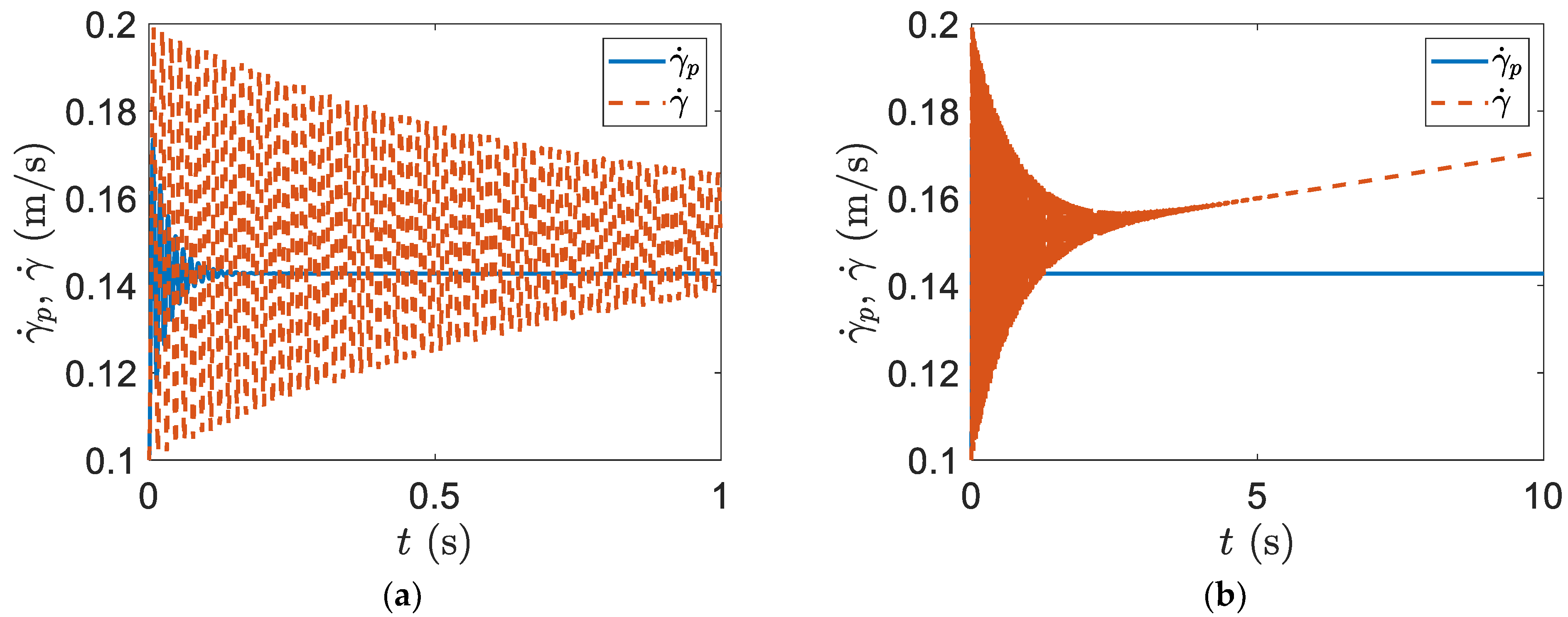
In this paper, it has been shown how by using piezoelectric patches and considering the blade rotational effect, the flutter can be delayed on a smart blade. Section 2 represents a smart blade system response with only plunge and rotational DOFs. Clearly, the oscillations of the smart blade can be effectively decayed in a very short time by implementing efficient flapwise and edgewise piezopatches. Almost in $0.4 \mathrm{s}$, the vibration of the smart blade flapwise velocity with only plunge and rotational DOFs can be decayed. However, the vibration of the regular blade flapwise velocity without a piezoelectric patch needs around $12 \mathrm{s}$ to decay. 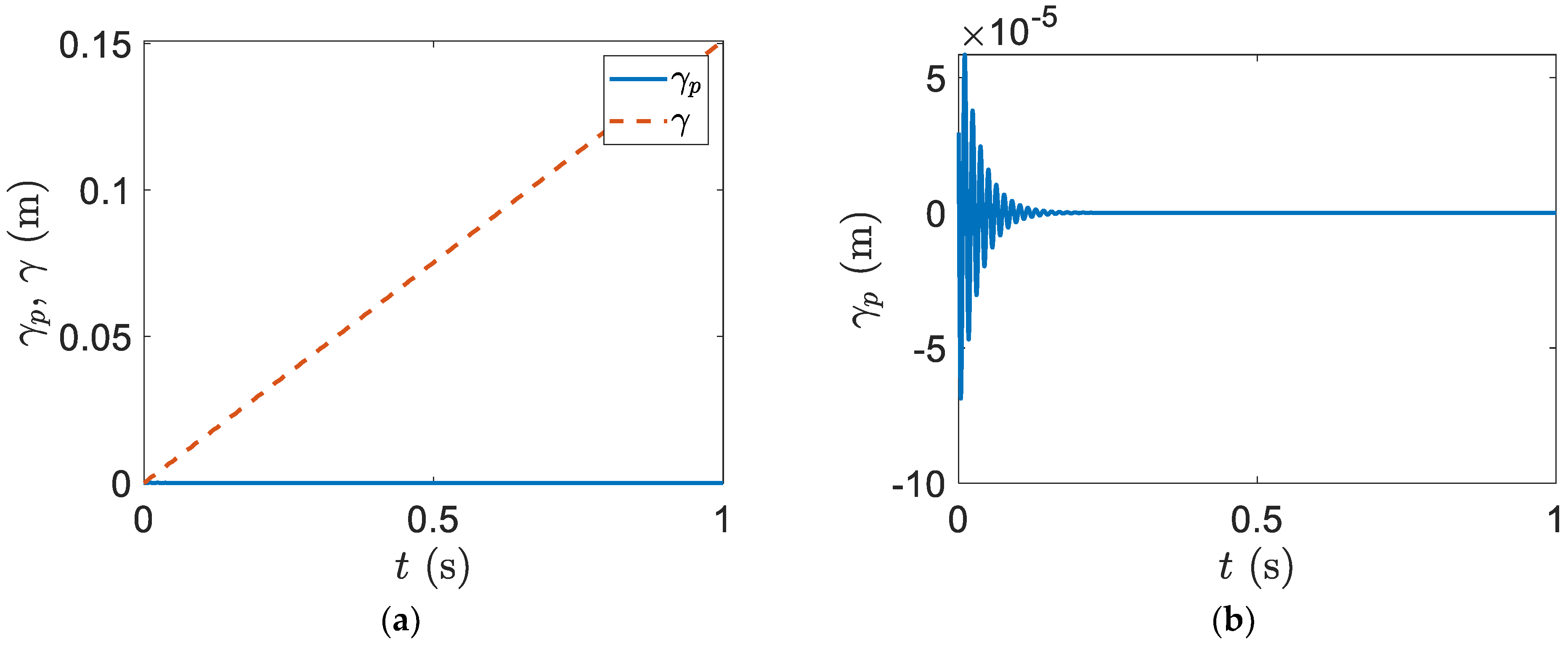Furthermore, the vibration of the smart blade edgewise velocity with only plunge and rotational DOFs can be decayed in $0.2 \mathrm{s};$ however, the vibration of the regular blade edgewise velocity without a piezoelectric patch needs around $8 \mathrm{s}$ to decay. In addition, in $0.4 \mathrm{s}$, the vibration of the smart blade flapwise displacement with only plunge and rotational DOFs can be decayed; however, the vibration of the regular blade flapwise displacement without a piezoelectric patch needs around $12 \mathrm{s}$ to decay. Moreover, the vibration of the smart blade edgewise displacement with only plunge and rotational DOFs can be decayed in $0.2 \mathrm{s}$; however, the vibration of the regular blade edgewise displacement without a piezoelectric patch needs around $10 \mathrm{s}$ to decay. In the rotational oscillation, the vibration of the smart blade rotational velocity with only plunge and rotational DOFs can be decayed in $0.15 \mathrm{s};$ however, the vibration of the regular blade rotational velocity without a piezoelectric patch needs around $5 \mathrm{s}$ to decay. Furthermore, the vibration of the smart blade rotational displacement with only plunge and rotational DOFs can be decayed in $0.2 \mathrm{s};$ however, the vibration of the regular blade rotational displacement without a piezoelectric patch needs around $1 \mathrm{s}$ to decay. As explained in Section 3, by using two piezopatches in the flapwise and edgewise plunge DOFs of a regular blade with three DOFs, the flutter speed can be postponed by $81.41\%$, which shows that the flutter speed is increased to a considerable value. Moreover, the results showed that how the flutter can shift from the flapwise plunge mode in a regular blade to the pitch mode in a smart blade. Later, it presents the effect of implementing one more piezopatch to a smart blade in the pitch DOF on the postponement of the flutter. The flutter speed in a smart blade can be postponed by $155\%$, which is a very considerable value.

References

1. Nguyen, N.T.; Ting, E.; Lebofsky, S. Aeroelastic Analysis of a Flexible Wing Wind Tunnel Model with Variable Camber Continuous Trailing Edge Flap Design. In AIAA Science and Technology Forum and Exposition (SciTech 2015); American Institute of Aeronautics and Astronautics: Reston, VA, USA, 2015. Available online: https://ntrs.nasa.gov/citations/20150021271 (accessed on 20 September 2022).
2. Hallissy, B.P.; Cesnik, C.E.S. High-Fidelity Aeroelastic Analysis of Very Flexible Aircraft. In AIAA Science and Technology Forum and Exposition (SciTech 2015); American Institute of Aeronautics and Astronautics: Reston, VA, USA, 2011; Available online: https://arc.aiaa.org/doi/abs/10.2514/6.2011-1914?cookieSet=1 (accessed on 20 September 2022).
3. Bisplinghoff, R.L.; Ashley, H.; Halfman, R.L. Aeroelasticity; Dover Publications: New York, NY, USA, 1996; Republication. [Google Scholar]
4. Fung, Y.C. An Introduction to the Theory of Aeroelasticity; Dover Publications: New York, NY, USA, 2008; Republication. [Google Scholar]
5. Dowell, E.H. A Modern Course in Aeroelasticity, 5th ed.; Springer International Publishing: Cham, Switzerland, 2015. [Google Scholar]
6. Hodges, D.H.; Pierce, G.A. Introduction to Structural Dynamics and Aeroelasticity, 2nd ed.; Cambridge University Press: Cambridge, UK, 2011. [Google Scholar]
7. Wright, J.R.; Cooper, J.E. Introduction to Aircraft Aeroelasticity and Loads, 2nd ed.; John Wiley & Sons, Ltd.: Hoboken, NJ, USA, 2015. [Google Scholar]
8. Moosavi, R.; Elasha, F. Smart Wing Flutter Suppression. Designs 2022, 6, 29. [Google Scholar] [CrossRef]
9. Verstraelen, E.; Gaëtan, K.; Grigorios, D. Flutter and Limit Cycle Oscillation Suppression Using Linear and Nonlinear Tuned Vibration Absorbers. In Proceedings of the SEM IMAC XXXV, Garden Grove, CA, USA, 30 January–2 February 2017. [Google Scholar]
10. Rocha, J.; Moniz, P.A.; Costa, A.P.; Suleman, A. On Active Aeroelastic Control of an Adaptive Wing Using Piezoelectric Actuators. J. Aircr. 2005, 42, 278–282. [Google Scholar] [CrossRef]
11. Olympio, K.R.; Poulin-Vittrant, G. A Honeycomb-Based Piezoelectric Actuator for a Flapping Wing MAV. In SPIE Smart Structures and Materials; Nondestructive Evaluation and Health Monitoring: San Diego, CA, USA, 2011. [Google Scholar]
12. Kucuk, I.; Yıldırım, K.; Adali, S. Optimal piezoelectric control of a plate subject to time-dependent boundary moments and forcing function for vibration damping. Comput. Math. Appl. 2015, 69, 291–303. [Google Scholar] [CrossRef]
13. Kuriakose, V.M.; Sreehari, V. Study on passive flutter control of damaged composite laminates with piezoelectric patches employing finite element method. Compos. Struct. 2021, 269, 114021. [Google Scholar] [CrossRef]
14. Bahaadini, R.; Saidi, A.R.; Majidi-Mozafari, K. Aeroelastic Flutter Analysis of Thick Porous Plates in Supersonic Flow. Int. J. Appl. Mech. 2019, 11, 1950096. [Google Scholar] [CrossRef]
15. Muc, A.; Flis, J.; Augustyn, M. Optimal Design of Plated/Shell Structures under Flutter Constraints—A Literature Review. Materials 2019, 12, 4215. [Google Scholar] [CrossRef] [PubMed] [Green Version]
16. Lossouarn, B.; Aucejo, M.; Deü, J.-F.; Multon, B. Design of inductors with high inductance values for resonant piezoelectric damping. Sens. Actuators A Phys. 2017, 259, 68–76. [Google Scholar] [CrossRef] [Green Version]
17. Zheng, C.; Song, H.; Liang, F.; Jin, Y.; Wang, D.; Tian, Y. 21st Century Maritime Silk Road: Wind Energy Resource Evaluation; Springer: Singapore, 2021. [Google Scholar]
18. Zheng, C.W.; Li, C.L.; Pan, J.; Liu, M.Y.; Xia, L.L. An overview of global ocean wind energy resource evaluations. Renew. Sustain. Energy Rev. 2016, 53, 1240–1251. [Google Scholar] [CrossRef]
19. Dimitriadis, G. Introduction to Nonlinear Aeroelasticity; Wiely: Hoboken, NJ, USA, 2017. [Google Scholar]
20. Theodorsen, T. General Theory of Aerodynamic Instability and the Mechanism of Flutter. NASA Ames Res. Cent. Class. Aerodyn. Theory 1934, 291–311. [Google Scholar]
21. Lee, B.; Price, S.; Wong, Y. Nonlinear aeroelastic analysis of airfoils: Bifurcation and chaos. Prog. Aerosp. Sci. 1999, 35, 205–334. [Google Scholar] [CrossRef]
22. Lee, B.; Gong, L.; Wong, Y. Analysis and computation of nonlinear dynamic response of a two-degree of freedom system and its application in aeroelasticity. J. Fluids Struct. 1997, 11, 225–246. [Google Scholar] [CrossRef]
Figure 1. A smart blade with flapwise and edgewise plunge and rotational DOFs.
Designs 06 00098 g001
Figure 2. The smart blade system responses of the velocity: (a) flapwise oscillation; (b) edgewise oscillation.
Designs 06 00098 g002
Figure 3. The smart blade system responses of the displacement: (a) flapwise oscillation; (b) edgewise oscillation.
Designs 06 00098 g003
Figure 4. Phase plane for the velocity and the displacement: (a) flapwise trajectory; (b) edgewise trajectory.
Designs 06 00098 g004
Figure 5. Phase planes for the electrical current and the charge: (a) flapwise trajectory; (b) edgewise trajectory.
Designs 06 00098 g005
Figure 6. The smart blade system responses of the rotational velocity: (a) time interval (0, 1) s; (b) time interval (0, 10) s.
Designs 06 00098 g006
Figure 7. The smart blade system responses of the rotational displacement: (a) the rotational displacement of smart and regular blades; (b) the rotational displacement of smart blade.
Designs 06 00098 g007
Figure 8. The smart blade system responses of the rotational displacement with P = 0 .
Designs 06 00098 g008
Figure 9. A smart blade with plunge, pitch, and control DOFs and a piezopatch in flapwise plunge DOFs.
Designs 06 00098 g009
Figure 10. Damping ratio versus airspeed: (a) regular blade; (b) smart blade.
Designs 06 00098 g010
Figure 11. Eigenvalues real part versus airspeed: (a) regular blade; (b) smart blade.
Designs 06 00098 g011
Figure 12. Eigenvalues imaginary part versus airspeed: (a) regular blade; (b) smart blade.
Designs 06 00098 g012
Figure 13. The smart blade unsteady plunge−pitch−control mode shapes at U = 10   m / s : (a) ω n = 6.8   Hz ; (b) ω n = 10.3   Hz ; (c) ω n = 17.7   Hz .
Designs 06 00098 g013
Figure 14. The smart blade unsteady plunge−pitch−control mode shapes at U = 74.2973   m / s : (a) ω n = 4.0   Hz ; (b) ω n = 10.2   Hz ; (c) ω n = 15.5   Hz .
Designs 06 00098 g014
Figure 15. A smart blade with plunge, pitch, and control DOFs and piezopatches in plunge and pitch DOFs.
Designs 06 00098 g015
Figure 16. The smart blade damping ratio versus airspeed with plunge piezopatches (a) and plunge and pitch piezopatches (b).
Designs 06 00098 g016
Figure 17. Eigenvalues real part versus airspeed: (a) smart blade with plunge piezopatches; (b) smart blade with plunge and pitch piezopatches.
Designs 06 00098 g017
Figure 18. Eigenvalues imaginary part versus airspeed: (a) smart blade with plunge piezopatches; (b) smart blade with plunge and pitch piezopatches.
Designs 06 00098 g018
Figure 19. Mode shapes of the smart blade in unsteady plunge, pitch, and control at U = 10   m / s : (a) ω n = 3.5   Hz ; (b) ω n = 2.7   Hz ; (c) ω n = 6.8   Hz .
Designs 06 00098 g019aDesigns 06 00098 g019b
Figure 20. Mode shapes of the smart blade in unsteady plunge, pitch, and control at U = 104.4198   m / s : (a) ω n = 1.9   Hz ; (b) ω n = 6.9   Hz ; (c) ω n = 9.6   Hz .
Designs 06 00098 g020aDesigns 06 00098 g020b
Publisher’s Note: MDPI stays neutral with regard to jurisdictional claims in published maps and institutional affiliations.