Abstract
A local scale Aerothermodynamic Generic Cycle Model (AGCM) is proposed. The AGCM accounts for several improvements not considered in similar models, such as compressor bleed extraction for aircraft Environmental Control System (ECS), parasitic shaft power extraction, and the enthalpy of the fuel entering the combustor. The AGCM is intended for steady-state Design Point (DP) and Off-Design (OD) performance analyses. The underlying physics is presented for the DP model. The turbomachinery component maps scaling and the system of nonlinear equations necessary to define the OD model are thoroughly discussed. The AGCM is compared with an equivalent model developed in the Numerical Propulsion System Simulation (NPSS). The comparisons were performed considering a DP envisioned to approximate a General Electric CF34-8C5B1 engine. The average errors found in these comparisons for the Specific Fuel Consumption (SFC) and net thrust were −0.111% and 0.193%, respectively. Finally, the predictions of the absolute levels of performance intended for the -8C5B1 engine are compared with empirical correlations derived from a comprehensive turbofan engine database. It was found that the predictions of the AGCM are in agreement with the empirical correlations; the errors found in SFC and net thrust at cruise flight condition were −0.43% and 2.06%, respectively.
1. Introduction
Simulation models of Gas Turbine Engines (GTEs) are key tools that predict their performance characteristics. For aero-propulsion applications, Fn and the Specific Fuel Consumption (SFC), are of utmost significance.
Several multidisciplinary studies for aircraft and engine models have been pursued in the Laboratory of Applied Research in Active Control, Avionics and AeroServoElasticity (LARCASE) [1]. Regarding engine models, the LARCASE has explored techniques, such as system identification [2,3], empirical equations [4], component level modeling [5], neural networks [6,7], etc., to predict the Fn and SFC for real engines, such as the Rolls-Royce AE3007C and the General Electric (GE) CF34-8C5B1.
Although novel methods have been explored, physics-based models are the ones most commonly used to predict the performance of GTEs. According to the literature review, the first computer physics-based simulation models date from the late 1960s and early 1970s [8,9,10]. Indeed, the offer of physics-based models has become ample over the years mainly due to the significant boost in computing capabilities.
Nowadays, robust and accurate physics-based models are typically developed on high-fidelity platforms such as the Numerical Propulsion System Simulation (NPSS) [11], GasTurb [12], GSP [13], and PROOSIS [14,15]. On the other hand, it is worth noting the progress made at Local Scale (LS), i.e., universities and research laboratories, to generate their own high-fidelity models for systematic research. For example, GSP and PROOSIS, before becoming professional commercial platforms, were developed at universities, such as the Technical University Delft (Delft, Netherlands) and the National Technical University of Athens (Athens, Greece), respectively. Other LS models found in the literature review include TSHAFT (U. of Padova, Padova, Italy) [16], Onyx (U. Toledo, Toledo, OH, USA) [17], T-MATS (NASA, Cleveland, OH, USA) [18], and C-MAPSS (NASA, Cleveland, OH, USA) [19]. Most of these LS models are available to a limited audience; at the moment of submitting this manuscript, only T-MATS [18] is available to the general public, free of charge.
An accurate physics-based GTE model for propulsion must account for the variation of the thermodynamic properties of the gas (air and combustion products) with P and T, and its composition, e.g., Water-to-Air Ratio (WAR) and Fuel-to-Air Ratio (FAR). Additionally, as the gas path flows in GTEs occur at high-speed, the compressibility effects in the thermodynamic properties must also be considered. Furthermore, the models must account for other effects that will take place during real operation, such as compressor bleed and shaft power extraction, which are of paramount importance to satisfy aircraft operational needs, e.g., the bleed extraction is used to supply the aircraft’s Environmental Control System (ECS). Additionally, cooling flow for the engine’s hot section (combustor and turbines) needs to be considered. On top of these characteristics, robust GTE aerothermodynamic models consider the capability to model Design Point (DP) and Off-Design (OD) performance.
The DP performance analyses are of interest during preliminary engine design phases when sizing the optimal engine. Several engine design characteristics are assessed to optimize the thermodynamic cycle based on technology limitations (e.g., materials, aerodynamics, cooling, etc.). Moreover, DP analyses are also suitable when aiming to approximate the aerothermodynamic DP of an engine already designed and built (as discussed later in this work).
Once the engine DP is fixed, and thus, the engine has been sized (i.e., the frontal and exhaust areas of the engine are known), it is crucial to understand its performance at different power settings ‘off’ from the DP, hence, the term ‘Off-Design’. Given that, in real operation, the propulsion engine is subjected to different power regimes (e.g., take-off, climb, cruise, idle, etc.) throughout its flight envelope, an OD model is needed to characterize its performance in such regimes.
In this paper, an Aerothermodynamic Generic Cycle Model (AGCM) is proposed first. The AGCM was completely developed in-house at the LARCASE using Matlab, and it is intended to run both DP and OD Steady-State (SS) simulations of GTEs for propulsion. The AGCM can simulate both high-pressure compressor bleed and shaft power extractions, the former is intended for ECS and turbine cooling, the latter satisfies aircraft and engine parasitic power demands.
While some of the LS models in the literature review, e.g., C-MAPSS [19] and T-MATS [20], suggest having the capability to account for compressor bleed extraction for ECS, it is not explicitly considered in their results. Indeed, bleed extraction for ECS has a significant penalty in SFC, given that the flow stream has already been compressed significantly in the high-pressure compressor and then sent to the aircraft cabin, producing no useful work within the engine. Similarly, shaft power extraction is not explicitly considered in the examples provided in these references, which also has a significant impact on engine performance (as discussed later in this work).
The AGCM also accounts for the hfuel entering the combustor. During real operation of modern turbofan engines, the fuel is used for thermal management purposes (i.e., cooling engine oil and aircraft components) before entering the combustor. The Δhfuel increase due to ΔTfuel is significant, about 1% of the fuel Lower Heating Value (LHV), which directly translates to a benefit in SFC of 1%. From the LS models mentioned above, it is not evident they account for Δhfuel either. However, it can be established that some of these models completely disregarded Δhfuel from their formulations, e.g., TSHAFT [16] and T-MATS [18].
The underlying thermodynamic calculations are developed for the AGCM-DP, and then these thermodynamic calculations are integrated with turbomachinery Component Maps (CMs) and a quasi-Newton numerical method to build the AGCM-OD. To assess the precision of the AGCM-OD, a comparison is made with an equivalent model programmed using the NPSS.
It is believed that a benchmark comparison against similar model(s) is key to generate credibility on any recent GTE model, although it is rarely encountered. Based on the literature review, few models have performed this benchmark comparison [14,18,21]; though, their comparisons are presented for a handful data points. In [14], only two SS data points (one at top of climb and other at sea-level static) are taken into account, whereas in [18,21], a single take-off point is considered in each study.
This work considered the comparison between the AGCM and NPSS models for a larger sample of points, comprising different flight conditions and power settings. Additionally, pertinent statistics are provided for the errors found in relevant performance parameters (e.g., SFC, Fn, Fg,pri, Fg,sec, NHcorr, etc.) which can be helpful for future model comparisons.
Finally, the AGCM is used to approximate the aerothermodynamic DP of a mid-size thrust engine, the GE CF34-85CB1. The assumptions of the DP are built based on a thorough literature review. The DP is used to define an OD performance model for the -8C5B1 engine, which is then compared with the empirical correlations proposed in [22]. These correlations are derived from a comprehensive database of commercial turbofan engines.
2. Model Description
The turbofan engine configuration characterized by the AGCM represents a two-spool separate exhaust turbofan engine (Figure 1). It is classified as a separate exhaust engine because the primary and the secondary streams each have their own exhaust nozzle.
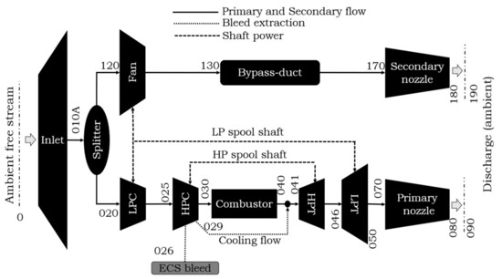
Figure 1.
Turbofan model schematic.
In Figure 1, the High-Pressure (HP) spool is formed by the HP Compressor (HPC) and the HP Turbine (HPT) connected by the same shaft. The Low-Pressure (LP) spool is given by the fan and the LP Compressor (LPC) connected to the same shaft as the LP Turbine (LPT). The turbofan engine also has a subsonic inlet, a single combustor, two convergent nozzles (primary and secondary), and a transition duct (bypass-duct) between the fan and the secondary nozzle. Moreover, the AGCM utilizes HPC bleed extraction for both ECS and HPT cooling, as well as HP shaft power extraction for customer (i.e., aircraft) and engine parasitic needs.
The nomenclature used herein to define a given parameter in the AGCM follows the pattern given in Figure 1, in which a numerical subscript is added to the parameter referring to a given station. For example, T0,040 is the total temperature at station 040 (i.e., at the exit of the combustor), is the corrected flow entering the engine (i.e., at station 0 or the ambient free stream). Similar nomenclature can be devised for other parameters.
The proposed AGCM is considered a zero-dimensional SS model, where no spatial and time-dependent variations in the thermodynamic properties of interest are considered; therefore, average thermodynamic properties at each station in Figure 1 are used. Aerothermodynamic zero-dimensional models show great capabilities and are widely used to address various GTEs problems: aircraft/engine optimization [23], specific engine matching [24], emissions assessment [25], engine diagnostics [26,27], etc.
The thermodynamic calculations in the AGCM consider the air and combustion products to behave as an ideal gas. Furthermore, to accurately calculate the thermodynamic properties of the air and combustion products, a set of tables proposed in [28] were included in the AGCM. The thermodynamic tables considered Φs from 0.0–1.0, WAR = 0.0 (i.e., dry air), and a fuel hydro-carbon ratio of 2.0. The Φ is defined as the ratio of the actual FAR to FARstoich, for example, Φ = 0.0 corresponds to dry air, and Φ = 1.0 to combustion products for FARstoich. The T and P ranges for the tabulated values are between 360–5400 R (200–3000 K), and 0.01–50 atmospheres, respectively. These tables also account for combustion products’ dissociation at high temperatures. The tabulated format is easy to use and inexpensive in terms of computational resources.
The compressibility effects in the flow path are considered by means of total thermodynamic properties (e.g., P0, T0, h0, etc.); however, the AGCM computes static properties (e.g., P, T, h, etc.) wherever flow areas are provided or calculated (e.g., engine inlet and nozzles discharge). Finally, the AGCM uses the ICAO Standard Atmosphere (SA) model [29] to compute P and T boundary conditions based on the geometric altitude.
2.1. Design Point Model
The aerothermodynamic calculations of each process in the AGCM-DP are presented in Appendix A. The calculations are performed sequentially from left-to-right according to Figure 1, first computing the secondary stream, then the primary stream. While most of the calculations are straightforward, few iterative processes are required to determine some of the unknowns (e.g., the FAR040 required to match T0,040, see Appendix A).
In the AGCM-DP, several characteristics that define the engine power (e.g., , β, compressive system PRs, T0,040, etc.) must be defined. Additionally, the figures of merit for the efficiency in each component must be specified (e.g., η, CV, ΔP/P, etc.). The main outcome of the DP is the prediction of the high-level performance (Fn and SFC); additionally, key information to size the engine is also obtained, i.e., nozzles’ exhaust areas (A080 and A180).
The AGCM-DP could be used, mainly, for two purposes: (1) to explore different engine thermodynamic cycle designs for new applications, and (2) to approximate the DPs of engines already designed and built. In this paper, the latter purpose is pursued.
2.2. Aerothermodynamic Design Point
One of the objectives of this work is to use the proposed AGCM to approximate the high-level performance of the CF34-8C5B1 engine. While any other engine approximation would have worked for the purpose of the comparison in this work, the -8C5B1 is of particular interest for LARCASE research.
The set of assumptions considered to approximate the DP of the CF34-8C5B1 engine are listed in Table 1, Table 2 and Table 3. These assumptions have been established based on a thorough literature review. The following paragraphs describe how these assumptions were obtained.

Table 1.
Top of Climb (TOC) assumptions.
Table 2.
Design Point (DP) engine component assumptions.
Table 3.
DP off-takes and cooling flow assumptions.
The aerothermodynamic DP considered in this work was assumed as the Top of Climb (TOC) at Cruise (CR) altitude (see Table 1). The TOC is typically the DP considered for commercial GTE aero-propulsion applications, given that is the condition at which the highest Overall PR (OPR), rotational corrected speeds, and inlet corrected flow are expected within the flight envelope [30].
The estimation of the maximum temperature of the thermodynamic cycle (i.e., T0,040) at TOC was threefold. First, the Fn,CR was determined at the minimum SFC condition. Second, the Fn,CR was scaled by 20% to determine the Fn corresponding to the TOC. The Fn,TOC is about 20 [31,32]—30% [30] higher than that of CR; in this work, 20% was considered. Third, the T0,040 associated with Fn,TOC was regarded as the throttle setting parameter (i.e., T0,040 = 2723.1 R, 1512.8 K) used to run the AGCM-DP.
The maximum PR for a single-stage fan is around 1.9 [32]; for this study, both the fan tip and hub PRs were assumed to be equal to 1.6. While the CF34-8C5B1 does not have an LPC [33], for modeling purposes in the AGCM, it was necessary to consider the fan tip and hub PRs separately, thus the compression of the fan hub stream was assumed to be performed by the LPC.
The β = 5.0 and the OPR = 28.0 values were obtained from the Original Engine Manufacturer (OEM) data presented in [34]. It is worth noting that, for obvious proprietary information reasons, the OEM does not specify to which flight condition both the β and OPR correspond, however, it was assumed that these numbers are representative of the engine aerothermodynamic DP. The HPC PR was obtained knowing that the OPR = PRHPC * PRLPC * PRInlet-duct. The PRInlet-duct was set to 1.0 (i.e., ΔP/PInlet-duct = 0.0), the reason behind this assumption is discussed later.
The estimation of the engine inlet total flow () was done considering the fan (tip and hub) inlet D010A and MN010A, the former equal to 46.2 in (1.17 m) [34] and the latter equal to 0.55 (average of the MN range (0.5–0.6) proposed in [35]). The estimated mass flow entering the engine was 177.11 lbm/s (80.34 kg/s). From the mass continuity equation, .
The LHVfuel is assumed to be 18,500 Btu/lbm (43,031 kJ/kg) per the OEM [33]. The hfuel was computed based on the Tfuel estimated at the combustor inlet. According to [36], the ΔTfuel when the engine is operating at high altitude could go to about 144 °F (80 °C), assuming Tfuel in the tank equal to 68 °F (20 °C), and at the combustor inlet, Tfuel = 212 °F (100 °C). A pressure average fuel enthalpy was calculated for JP-4 fuel in accordance with the information presented in [37] based on Tfuel at the combustor inlet, obtaining hfuel = 176 Btu/lbm (409.4 kJ/kg). The hfuel value represents 0.95% of the LHV, which is not negligible. A better prediction of the , and hence of the SFC, could be estimated when considering the hfuel, as discussed in this paper. Otherwise, both and SFC would be overpredicted by about 1.0%, which is significant for high-fidelity simulations.
The adiabatic efficiencies (η) of the turbomachinery components (e.g., compressors and turbines) were obtained from an engine design proposed by GE for the NASA Energy Efficient Engine (EEE) [38]. This design was aimed for an engine intended to be introduced in-service late 1980s to early 1990s. The CF34-8C5B1 obtained its FAA certification in 2002 [33], however it is believed that its design must have been conceived a decade earlier. Given that both engine designs belonged to the same OEM, it is likely they share similar technology (e.g., aerodynamics, cooling, materials, etc.).
The combustor efficiency (ηComb), it was also obtained from [38]. Regarding the combustor pressure loss (ΔP/P), it was assumed that the so-called ‘cold pressure loss’ played a dominant role in the overall pressure loss. Cold pressure loss is associated with the combustor diffuser and liner. A typical cold pressure loss for annular combustors (such as the one for the CF34-8C5B1 engine) is 6.0% [39].
As for the mechanical transmission efficiencies in both the HP and LP shafts, according to [32], the power loss could be up to 5% of that being transmitted in the spool (due to bearing friction and windage). An intermediate value of 2.5% was considered for both transmission efficiencies, hence ηHP,mech, ηLP,mech = 0.975.
Regarding the inlet and bypass ducts pressure losses, ΔP/P = 0.0 was assumed for both, as the same engine power plant can be used in different aircraft applications; for example, the CF34 engine is used in two aircraft applications: CRJ-700 and Embraer-170. Depending on the airframer, both the inlet and bypass duct can present different ΔP/P’s, thus it was assumed to use the uninstalled performance for DP purposes. However, the installation effects are considered for the OD comparisons, as detailed later.
During DP calculations, the nozzles’ exit areas must be resized to match the exit flow and the thermodynamic conditions, thus, the CD is intrinsically considered, and therefore CD,pri, CD,sec = 1.0. Regarding the CV, in [40] it was found empirically that for conic convergent nozzles, the CV is practically constant (CV = 0.945) in the range of PRs 1.3–1.8 (critical PR), thus CV,pri, CV,sec = 0.945.
Concerning the customer off-takes, such as ECS bleed extraction and HP shaft power extraction, they were set to zero due to the same reasons as for the inlet and bypass ducts ΔP/P’s. The parasitic off-takes (i.e., those necessary for the engine operation), such as parasitic power extraction for oil and fuel pumps, and HPC bleed extraction for turbine cooling are presented in Table 3.
The parasitic power extraction from the HP shaft was considered as 155 hp (115.6 kW) as in [33]. Regarding HPT cooling flow, 25% of the HPC flow was considered for cooling [30]. The total of the cooling flow is assumed to be non-chargeable, i.e., it will be reinstated to the main flow path upstream of the HPT (see Figure 1). Additionally, it was assumed the extraction P matches the HPT inlet P. The fractions , and were set to meet the intended flow and to comply with the second law of thermodynamics (e.g., ). The definitions of these fractions are presented in the compressor calculations in Appendix A.
2.3. Off-Design Model
The AGCM-OD inherited the thermodynamic calculations from the -DP model. However, some adjustments were made in the way in which the calculations are executed. As discussed previously, the DP calculations are rather straightforward, with few iterative processes. However, OD performance calculations are iterative in nature; the main objective during OD simulations is to obtain suitable operating points on each engine Component Map (CM), such that the mass and energy conservation within the engine is observed. At this stage in the AGCM, only turbomachinery CMs are considered (i.e., compressor and turbines).
A turbomachinery CM comprises a series of correlations that relate the overall thermodynamic parameters to its rotational speed. These correlations are presented based on corrected (or referred) parameters, which are a helpful tool to define a unique set of correlations regardless of the Pin and Tin boundary conditions at which the turbomachinery component is exposed. The corrected parameters are typically referred to as the Sea-Level (SL) condition by means of Equations (1) and (2), in which Tstd = 518.67 R (288.15 K) and Pstd = 14.696 psia (101.325 kPa).
The correlations defined in a typical compressor map are presented in Equations (3)–(5). These correlations are functions of the Ncorr and R-lines, the latter are auxiliary coordinates defined in a compressor map to uniquely define its operating point at a given power-setting. It is worth mentioning that the auxiliary coordinate can be defined in several ways, e.g., β-lines [41], however, for the compressor maps included in the AGCM, only R-lines were used. The definition of Ncorr is presented in Equation (6), in which θin represents the dimensionless corrected temperature at the inlet of the compressor in question.
For the turbine maps, the typical correlations are presented for the so-called Flow Function (FF) and ηTurb, Equations (7) and (8); these correlations are functions of the inverse of the PR (e.g., P0,in/P0,out) and the corrected turbine speed NP, Equation (9). The T0,in in Equation (9) represents the total temperature of the turbine in question.
In research work, it is highly likely that the turbomachinery CMs of the engine under analysis are not known. Indeed, CMs are proprietary information owned by OEMs, and thus are not broadly shared. However, researchers can cope with the lack of knowledge about the turbomachinery of a specific engine by scaling a known set CMs.
The AGCM-OD model uses a linear scaling method to project the turbomachinery CMs to represent engines of different sizes. In this scaling method, it is assumed that a given parameter X in a CM at the DP preserves a constant relationship (i.e., scalar) to that of the scaled application DP. The scalars are calculated by means of Equation (10), where X can represent Ncorr, NP, , FF, η. For the specific case of the PR, X = PR−1. Once the scalars are calculated, they remain fixed throughout the analysis.
To appropriately determine the operating points on each CM, the AGCM-OD uses an iterative process in which n-independent parameters, represented by the n-vector x, are varied such that Equation (11) holds. The m-vector ε in Equation (11) represents the mass and energy imbalance errors, and the expression represents its Euclidian norm. Each vector element εj is the error between the state and demand of a given yj in Equation (12). In Equation (11), μ represents a convergence tolerance, which was set to μ = 1 × 10⁻⁵ in the present study. The set of xi and yj defined in the -OD model is presented in Table 4.
Table 4.
Aerothermodynamic Generic Cycle Model (AGCM) independent and dependent parameters.
To find the solution vector x* that satisfies Equation (11), a series of iterations must be performed. The attempt to find x* begins with an educated initial guess of the solution, x0, then at the kth + 1 iteration, an improved value of x is computed by means of Equation (13), in which p represents the step direction from the current iterate xk, and α stands for the step size. The vector p is computed by solving a system of m = n nonlinear equations given by Equation (14), in which J is an mxn square matrix that is composed by the , Equation (15). α is nonnegative scalar computed by means on an inexact line search method.
For thermodynamic cycle modeling, calculating J in every kth iteration is a time-consuming task, given that to compute the mth gradient, (i.e., each row in J), the calculations of the whole cycle model (see Appendix A) must be executed m + 1 times.
To improve the execution time in the kth + 1 iteration, the Jk + 1 in Equation (14) is replaced by Bk + 1, the latter approximates the J precluding computing the . The numerical methods that make an approximation of J are called quasi-Newton or secant methods. The Bk + 1 is computed by the so-called Broyden formulae [42], presented in Equation (16). Bk + 1 is obtained by an inexpensive vector-matrix computation that depends on Bk, Δxk, and Δεk, the latter two defined in Equations (17) and (18), respectively. In [43], it is reported that the quasi-Newton method is, on average, 55% faster than a Matlab ‘off-the-shelf’ non-linear least square method.
Finally, it should be noted that for the quasi-Newton method implemented in the AGCM-OD, J had to be calculated in the first iteration (i.e., J0) or when no sufficient progress towards the solution was made, as defined in Equation (19), in which τ has been arbitrarily set to 0.10. The quasi-Newton numerical method algorithm programmed in the AGCM is shown in Figure 2.
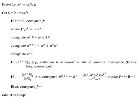
Figure 2.
Quasi-Newton method iteration algorithm.
2.4. Model Comparison
To benchmark the precision of the AGCM-OD, a comparison was made with an equivalent model programmed in the NPSS. To prevent any systematic bias in this comparison, the NPSS model showed the same characteristics of the turbofan engine depicted in Figure 1; additionally, the DP assumptions reflected in Table 1, Table 2 and Table 3 were also utilized in the NPSS model. For the OD computation, both the NPSS and the AGCM used the same CMs considering linear scaling. Finally, the NPSS model was run with the so-called ‘allFuel’ thermodynamic package, which according to [44], ‘is generally consistent’ with the US customary units’ version of the thermodynamic tables provided by [28] and implemented in the AGCM. A comparison was made to assess the alleged ‘consistency’ between these sets of tables. Indeed, the absolute values for h and s are not the same between NPSS ‘allFuel’ (after the units’ conversion to SI) and [28], however, similar derivatives in h vs. T and s vs. T were observed at constant P and Φ, i.e., and . It should be noted that for thermodynamic calculations, what matters is the ΔZ from the thermodynamic state A to B, rather than the absolute values of Z in A and B. To perform a quantitative comparison of these derivatives, the absolute levels of h and s from [28] were normalized relative to the NPSS ‘allFuel’ tables utilizing the corrections shown in Table 5. The temperature used to define the corrections was Tstd, and the corrections were invariant of P.
Table 5.
Thermodynamic properties corrections.
The comparisons of the properties of interest (e.g., h, s, γ, R) between NPSS ‘allFuel’ and [28] after normalization are presented in Figure 3. The small errors shown in Figure 3 (less than ±0.2% for 400 ≤ T ≤ 3000 R or 222.2 ≤ T ≤ 1666.7 K) indicate that the derivatives between both sources of thermodynamic properties are alike, and thus consistent.
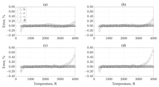
Figure 3.
Numerical Propulsion System Simulation (NPSS) ‘allFuel’ thermodynamic package vs. [28] (P = 1.0 atm). (a) Φ = 0.0 (upper-left), (b) Φ = 0.25 (upper-right), (c) Φ = 0.50 (lower-left), (d) Φ = 0.75 (lower-right).
The comparison between the two OD models was done based on three representative flight conditions, one on-ground and two in-flight, according to the conditions listed in Table 6. The engine power setting parameter was considered as the NLcorr with steps of ΔNLcorr = 2.5%. At each flight condition, two temperature levels were considered, one for ΔTICAO-SA = 0.0 °F (0.0 °C) and the other for a representative corner point temperature in turbofan commercial applications, e.g., ΔTICAO-SA = 27.0 °F (15.0 °C) for SL and ΔTICAO-SA = 18.0 °F (10.0 °C) for both flight conditions. In this comparison, the pressure losses for the inlet and bypass ducts, as well as the bleed extraction for ECS were considered and are discussed next.
Table 6.
Flight conditions for model comparison.
For the inlet duct, the ΔP/Pinlet-duct = 0.34% was obtained from a relationship of ΔP/P vs. MNTh presented in [35] assuming a MNTh = 0.70. Regarding the bypass duct, it was assumed ΔP/Pbyapss-duct = 2.4% based on Equation (20) [31].
The bleed extraction was set to 1.32 lbm/min (0.60 kg/min) per passenger [32]. The CF34-8C5B1 powers the CRJ-700; this aircraft has a capacity of 73 total passengers (68 passengers plus 5 crew members) [45], and each plane is powered by two -8C5B1 engines. The calculated bleed extraction per engine was 48.18 lbm/min (21.85 kg/min). The corresponding mass fraction was = 0.0272.
To define the PR at the extraction port (i.e., station 026 in Figure 1), it was assumed that the bleed was extracted from the 6th stage (out of 10 compression stages), as in [33]. Additionally, assuming that each compression stage provides the same PR, and knowing the HPC PR = 17.5 (see Table 1), then, at the 6th stage, the PR = 10.5. Finally, the Pf,ECS and wf,ECS were set to 0.5758 and 0.7569, respectively. Similar to the fractions for HPT cooling, Pf,ECS and wf,ECS were set to comply with the second law of thermodynamics (e.g., ).
It is worth mentioning that during real engine operation, the HPC bleed extraction for ECS switches between intermediate pressure (6th stage, station 026 in Figure 1) and compressor discharge (station 030 in Figure 1). For mid-to-high power operation, the bleed is extracted from the former and at low power settings from the latter. In this work, on both the AGCM and NPSS models, the ECS bleed was extracted from the intermediate pressure port regardless of the power setting. The current version of the AGCM does not allow to switch between pressure ports.
Lastly, the predictions of the CF34-8C5B1 obtained from the AGCM were compared with the correlations proposed by [22]. Indeed, engine data is difficult to obtain for research purpose unless there is a specific agreement with an OEM to obtain such data, otherwise researchers rely on data publicly available. The correlations provided in [22] were used to obtain a realistic reference to compare the high-level performance absolute values, such as Fn and SFC, for the -8CB1 approximation. These correlations were derived from an engine database of commercial turbofan engines; they provide average performance estimates based on engine size (e.g., fan diameter) and power (e.g., thrust at take-off). The set of correlations from [22] was adapted and are presented in Equations (21)–(27).
3. Results Discussion
The results discussion begins with the maximum temperature of the thermodynamic cycle used in the DP, T0,040. According to Table 1, the T0,040 at TOC was 2723.1 R (1512.8 K). It is of utmost importance to determine if this temperature is representative of the CF34-8C5B1 engine.
The temperatures at the exit of the combustor are not typically available in the literature, except in wide ranges, thus the HPT inlet temperature (T0,041) was used as surrogate for comparison. The T0,041 obtained in the present design was compared against its equivalent temperature from [38], the former equal to 2384.7 R (1324.8 K) and the latter to 2799.3 R (1555.2 K). The observed ΔT0,041 between both designs, taking [38] as reference, was −414.6 R (−230.4 K) which was deemed significant.
While both designs considered the same turbomachinery and combustor efficiencies, there are differences in other assumptions that produced the significant gap in ΔT0,041. For example, it was found that the differences in HPC PR and β were responsible for most of the observed ΔT0,041. In [38], the HPC PR and β were set to 23.0 and 6.8, respectively, whereas in this study, these parameters were equal to 17.5 and 5.0, respectively. The ΔHPC PR and Δβ are equal to −31.4% and −26.0%, respectively.
Table 7 presents the contribution of HPC PR and β differences to the ΔT0,041, the former contributes 55.8 R (31.0 K) and the latter 322.3 R (179.1 K), thus, the total contribution from both is 378.1 R (210.1 K). These results suggest that when correcting for the HPC PR and β differences, the T0,041 in the present study becomes significantly closer to the one in [38], reducing ΔT0,041 to −36.5 R (−20.3 K). It was concluded that the T0,040 = 2723.1 R (1512.8 K) used in this work was deemed reasonable based on the assumed HPC PR and β.
Table 7.
Assumption differences vs. [38].
The second part of our discussion is centered in the CMs scalars used to approximate the CF34-8C5B1. The scalars presented in Table 8 were computed per Equation (10) based on the DP approximation of the -8C5B1 engine and the DP of the CMs in the AGCM. It should be noted that these CMs are intended for a bigger engine (i.e., higher rated thrust and total corrected flow) than that of the CF34-C5B1.
Table 8.
Turbomachinery components scaling factors (dimensionless).
The scalars represent a deviation in a parameter of the current map (e.g., η, PR, etc.) to match the same parameter on the intended design (i.e., the CF34-8C5B1). When a significant difference exists between the aforementioned parameters, the scalar tends to deviate, significantly, from unity. For example, in the case of the corrected fan and HPC flow scalar, the corrected flow estimated in these components for the CF34-8C5B1 at DP was 380.93 lbm/s (172.79 kg/s) and 51.31 lbm/s (23.27 kg/s), respectively, whereas the corrected flow in the fan and HPC maps at DP were 1441.71 lbm/s (653.95 kg/s) and 123.57 lbm/s (56.05 kg/s), respectively. Thus, the flow in the fan and HPC maps had to be reduced by 73.6% and 58.5%, respectively, to match the desired intent. As noted previously, researchers need to cope with the limited CMs data available, thus it is not uncommon to observe scalars that deviate significantly from unity, e.g., [21].
The comparison of the AGCM-OD and NPSS results is discussed next. The errors for the high-level performance were computed, taking as reference the NPSS model. Figure 4 presents the errors for , Fn, Fg,pri, Fg,sec, , NHcorr, , and for the ‘Ground’ condition across engine power (i.e., NLcorr). This comparison comprises the average values obtained from ΔTICAO-SA equal to 0.0 and +27 °F (+15 °C).
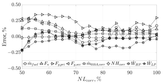
Figure 4.
Average errors (ΔTICAO-SA = 0.0 and +27 °F/+15 °C) vs. NLcorr (‘Ground’ condition).
In Figure 4, it is clear the errors are fairly distributed around zero, i.e., they do not present an apparent correlation with NLcorr, which was expected, given that, as discussed in Section 2.4, any systematic bias between models was deliberately precluded.
Next, the errors are compared for the different flight conditions considered in Table 6. Figure 5, Figure 6 and Figure 7 present the key statistics for the errors on each flight condition, which include the average, ±t95σ, and Maximum Absolute Error (MAE). It is worth noting that the SFC comparison was computed at constant Fn, in contrast to the other parameters (e.g., Fn, , etc.), for which the errors were calculated at constant NLcorr. The statistics were computed throughout the NLcorr power range considering both temperature levels on each flight condition, thus the sample sizes for ‘Ground’, ‘Flight 1’, and ‘Flight 2’ were n = 42, n = 36, n = 28, respectively. The value of ±t95σ is a measure of the model precision, i.e., 95% of the computed errors should fall within this range. The t95 value is a suitable statistic for a small sample size, e.g., n ≤ 30. For large samples, the t95 approaches asymptotically to 2.0, i.e., the value of a normal distribution. The corresponding t95 values for these conditions were 2.018, 2.028, and 2.048, respectively. The σ corresponds to the sample standard deviation of the errors. The MAE is a measure of the extreme error found in the comparison, and which, as noted in Figure 5, Figure 6 and Figure 7, can be outside the ±t95σ range.
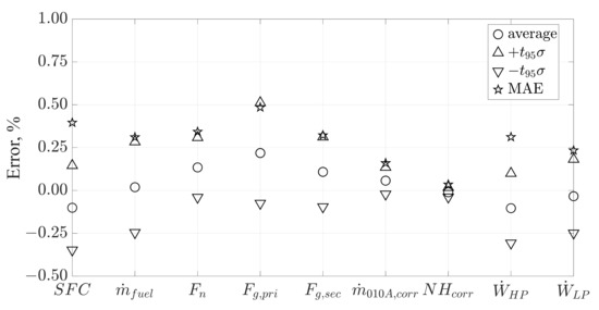
Figure 5.
‘Ground’ condition error statistics (n = 42).
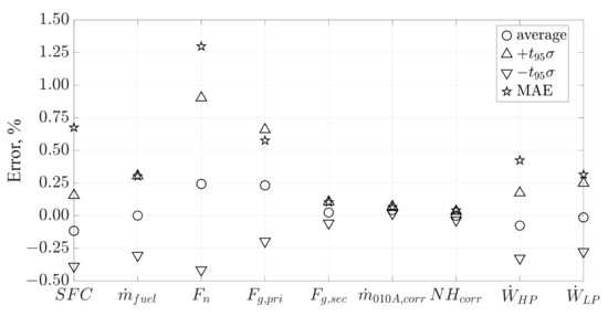
Figure 6.
‘Flight 1’ condition error statistics (n = 36).
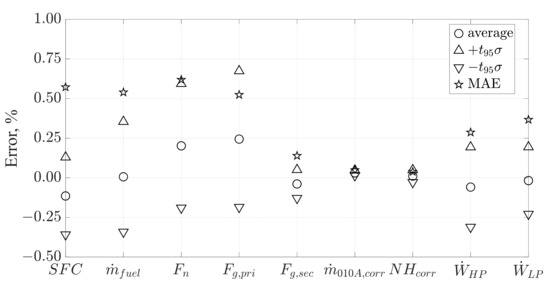
Figure 7.
‘Flight 2’ condition error statistics (n = 28).
Overall, the errors observed in Figure 5, Figure 6 and Figure 7 are considered small and acceptable; for example, the average SFC and Fn for the three flight conditions in Table 6 were −0.111% and 0.193%, respectively. The highest ±t95σ and MAE values were observed for Fn at the ‘Flight 1’ condition, which is explained by the small absolute values Fn obtained at low power conditions. For example, at NLcorr = 57.5% and ΔTICAO-SA = 0.0 °F (0.0 °C), the Fn = 314.8 lbf (1400.3 N), thus 1.0% of Fn is 3.1 lbf (14 N).
The errors shown in these comparisons could be used as a reference to compare (or validate) aerothermodynamic cycle models for propulsion, given that, as mentioned previously, the comparisons found in similar models [14,18,21] do not consider all the parameters shown in Figure 5, Figure 6 and Figure 7, in particular SFC. Moreover, the comparisons in the aforementioned references rely on limited data points, e.g., two data points (SLS and TOC) in [14], and a single take-off data point in [18,21].
While the comparisons between models shown hitherto have considered all the modeling characteristics that differentiate the AGCM from other LS models, e.g., ECS bleed extraction, HP shaft power extraction, and hfuel, these comparisons do not provide information about the impact of these factors on the overall performance; this is addressed next. Table 9 summarizes the impact of not considering these factors. The figures in this table were computed taking as reference the scenario in which these three factors are considered, i.e., , hp (115.6 kW), and hfuel = 176 Btu/lbm (409.4 kJ/kg).
Table 9.
, , hfuel impact on performance.
Table 9 shows that the ΔSFCs are significant. For example, ignoring, deliberately or by omission, both the ECS bleed and HP shaft power extractions, i.e., and , the SFC predictions would improve by 3.59% and 1.53%, respectively. These overly optimistic figures could be a cause of trouble when simulating, for example, the fuel consumption throughout an aircraft’s flight mission. Additionally, neglecting the hfuel effect, the SFC would be incorrectly penalized by 0.97%, which is also a significant figure. When the fuel is used for thermal management purposes, the simulations should take credit for the SFC improvement due to the increased hfuel.
It is worth mentioning that there could be scenarios in which some of these assumptions could be disregarded, for example, ECS bleed extraction is not considered for uninstalled performance predictions (as discussed later in this work), or when simulating an engine in a test cell stand. However, it is better to have a model that could consider them whenever necessary rather than not at all.
The final part of the discussion results is focused on the CF34-8C5B1’s absolute levels of performance predicted by the AGCM compared to those of the correlations provided in [22]. It should be noted that several drawbacks arise when these correlations are used; for example, one cannot be certain which flight conditions (e.g., altitude, MN¸ ΔTICAO-SA) and assumptions (e.g., installed vs. uninstalled) were used to define the engine performance data from which these correlations were derived.
In the case of the AGCM predictions, uninstalled performance was considered (i.e., no ECS bleed extraction, and 100% recovery for inlet and bypass ducts). The TKOF flight condition was set to SL static (MN = 0.0), ΔTICAO-SA = 0.0 °F (0.0 °C), and the Fn was set equal to the CF34-8C5B1 Normal Take-Off thrust rating, i.e., Fn,TKOF = 12,670 lbf (56,359 N) [33]. In the case of CR, the altitude and MN were the same as ‘Flight 2’ in Table 6 with ΔTICAO-SA = 0.0 °F (0.0 °C). The Fn setting at CR was set as the corresponding to NLcorr = 100.0%, i.e., Fn,CR = 2790.4 lbf (12,412.3 N). The correlations presented in Equations (21)–(27) were evaluated at Fn,TKOF = 12,670 lbf (56,359 N).
The comparison of the -8C5B1 predictions by the AGCM and those of the correlations in [22] are presented in Table 10. It should be noted that for the AGCM, Dfan is not obtained from computation, but instead is an input used to define in Table 1. The Dfan obtained from the correlations agrees with the value used in the model calculations (ΔDfan = 0.65%). Moreover, the small error in ( = 3.86%) is linked to the Dfan considered in the AGCM calculations.
Table 10.
Performance absolute levels comparison (CF34-8C5B1 engine prediction, AGCM vs. [22]).
The errors for β, OPR, and SFCTKOF seem contrasting compared to other parameters, although, when comparing their absolute values with the individual data points from which the correlations were derived (see Figure 8), the predictions of the AGCM are well within the family of data points. In other words, other data points in the population show similar or even higher errors relative to the correlation line.
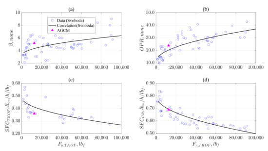
Figure 8.
Performance comparison, Aerothermodynamic Generic Cycle Model (AGCM) vs. [22]. (a) β vs. Fn,TKOF, (b) OPR vs. Fn,TKOF, (c) SFCTKOF vs. Fn,TKOF, (d) SFCCR vs. Fn,TKOF.
Regarding the SFCTKOF, it can be observed in (Figure 8c) that the sample of data points is 35% smaller and has a greater scatter than that of SFCCR (Figure 8d); thus a higher error is expected in the former. Nonetheless, the AGCM predictions for SFCTKOF are within the cluster of points grouped between Fn: 5700–14,200 lbf (25.4–63.2 × 10³ N) in Figure 8c, suggesting that this prediction is within expectations.
Concerning the errors in Fn,CR and SFCCR, these are considered small and acceptable; in the case of the latter, Figure 8d shows its good agreement with the correlation line. Finally, according to the OEM specifications in [34], the SFCCR is quoted as 0.67 lbm/h/lbf (0.0683 kg/h/N). The error relative to this specification is 2.8%, which was also considered acceptable.
The results obtained throughout this work suggest that the DP assumptions, CMs scalars, and high-fidelity aerothermodynamic modeling of the AGCM seem to reasonably approximate the absolute levels of performance expected of an engine of the size and thrust of a CF34-8C5B1.
4. Conclusions and Final Remarks
The high-fidelity AGCM presented in this work is able to perform both DP and OD performance calculations accounting for effects such as compressor bleed extraction for aircraft ECS, shaft power extraction, and sensible enthalpy of the liquid fuel entering the combustor. These improved features are not explicitly encountered in similar LS models in the literature.
The AGCM presented in this work was compared with an equivalent model programmed in the high-fidelity platform NPSS, the average errors for the SFC and Fn found in this comparison were −0.111 and 0.193%, respectively. The statistics reported in this paper could serve as a reference for similar comparisons of other GTE aerothermodynamic models for propulsion.
The set of DP assumptions considered to approximate the CF34-8C5B1 engine and the turbomachinery scalars resulted in performance absolute value predictions that were considered in agreement with the expectations derived from empirical correlations. The errors for the SFC and Fn at cruise conditions were −0.43% and 2.06%, respectively. Moreover, the error in the SFC at cruise with respect to that reported by the OEM was 2.8%.
Lastly, it is expected that the results from this research will be used in the future to perform systematic research in GTE at the LARCASE. Specifically, to match the AGCM results to the CF34-8C5B1 engine data obtained from a high-fidelity Level D flight simulator, manufactured by CAE Inc. and located at the LARCASE.
Author Contributions
M.d.J.G.A.: Conceptualization, methodology, software, validation, data curation, formal analysis, investigation, and writing—original draft preparation. R.M.B.: Writing—review and editing, supervision, project administration, and funding acquisition. All authors have read and agreed to the published version of the manuscript.
Funding
This work was funded by the NSERC through the Canada Research Chair in Aircraft Modeling and Simulation Technologies.
Institutional Review Board Statement
Not applicable.
Informed Consent Statement
Not applicable.
Acknowledgments
This research was performed at the Laboratory of Applied Research in Active Controls, Avionics and AeroServoElasticity (LARCASE). For more information related to this research, please visit the LARCASE website at http://larcase.etsmtl.ca (accessed on 29 September 2022).
Conflicts of Interest
The authors declare no conflict of interest. The funders had no role in the design of the study; in the collection, analyses, or interpretation of data; in the writing of the manuscript; or in the decision to publish the results.
Nomenclature
| A | flow area | Greek letters | |
| c | speed of sound | α | step size |
| B | mxn Broyden matrix | β | bypass ratio |
| CD | flow coefficient | θ | dimensionless temperature |
| Cp | specific heat at constant pressure | δ | dimensionless pressure |
| Cv | specific heat at constant volume | η | efficiency |
| CV | velocity coefficient | Δ | difference |
| D | Diameter | Φ | equivalence ratio |
| FAR | Fuel-to-Air Ratio | mass flow bleed fraction | |
| Fg | gross thrust | λs | numerical tolerance |
| FF | Flow Function | τ | error function improvement tolerance |
| Fn | net thrust | γ | specific heat ratio |
| Fram | ram drag | σ | standard deviation |
| h | specific enthalpy | μ | convergence tolerance |
| J | mxn Jacobian matrix | ε | m-vector of errors |
| LHV | Lower Heating Value of the fuel | ρ | density |
| maxIt | maximum number of iterations | ζ | thermodynamic state |
| mass flow | Γ | scrubbing drag due to external engine wet surfaces | |
| MFP | Mass Flow Parameter | Subscripts | |
| MN | Mach Number | bleed | at bleed extraction port |
| n | sample size | cool | cooling |
| N | rotational speed | Comp | compressor |
| Ncorr | corrected rotational speed for a compressor | Comb | combustor |
| NLcorr | corrected rotational speed for the LP spool | corr | corrected |
| NHcorr | corrected rotational speed for the HP spool | cust | customer (i.e., aircraft) |
| NP | corrected rotational speed for a turbine | demand | demand of dependent parameter |
| p | step direction m-vector | fuel | parameter associated with the fuel entering the combustor |
| P | pressure | ideal | corresponding to ideal process |
| Pf | pressure bleed fraction | in | at the inlet of an engine component |
| PR | Pressure Ratio (i.e., PR = P0,out/P0,in) | mech | mechanical transmission |
| shaft power extraction | par | parasitic | |
| net heat transfer | pri | engine primary stream | |
| R | gas constant | out | at the exit of an engine component |
| R-line | auxiliary coordinate | real | corresponding to real process |
| s | specific entropy | sec | engine secondary (or bypass) stream |
| S | scaling factor | stoich | stoichiometric |
| SFC | Specific Fuel Consumption | state | state of the dependent parameter |
| t95 | inverse of student’s t distribution (95% confidence) | std | standard day condition |
| T | Temperature | Th | inlet duct throat |
| V | flow velocity | Turb | turbine |
| w | specific work (i.e., work per unit mass) | 0 | representing a total (or stagnation) thermodynamic property (e.g., h0, T0, P0) |
| wf | work bleed fraction | ||
| WAR | Water-to-Air Ratio | ||
| shaft power | |||
| x | n-vector of independent parameters | ||
| x* | solution n-vector | ||
| X | generic map parameter | ||
| y | m-vector of dependent parameters | ||
| Z | generic thermodynamic property (e.g., T, P, h, etc.) | ||
Appendix A
Table A1 summarizes the modeling of the aerothermodynamics processes that occur in the turbofan engine depicted in Figure 1. These calculations are intended for the -DP model, however, the reader might deduce the changes that need to take place for the -OD based on the information presented in Section 2.3. The ‘Inputs’ column of Table A1 refers to those parameters that are intended to be provided by the user. The ‘Modeling’ column details the aerothermodynamic modeling of each component based on the thermodynamic properties at the inlet of the component and the physics behind the process. The aim of the thermodynamic modeling is to find two independent properties that, along with the gas composition (i.e., FAR), allow to determine the thermodynamic state (ζ) at the end of the thermodynamic process, i.e., at the exit of the component. It should be noted that the ζ could be determined based on static or total thermodynamic properties. Given that in most of the engine components, there is no information (e.g., A or MN) to determine the static properties, the total properties are used; however, in components such as the ambient, the inlet duct (if fan diameter is provided), and both primary and secondary nozzles, the static properties are also computed. The nomenclature used to summarize the set of thermodynamic properties that are calculated once ζ is defined is as follows
[h, s, Cp, Cv, γ, R, c, ρ] = [static] = ζ(FAR, Z1, Z2)
The expression ‘[static]’ or ‘[total]’ in Equations (A1) and (A2), respectively, refers to the set of thermodynamic properties that are computed by the thermodynamic tables in the AGCM. The set of thermodynamic properties h, s, Cp, Cv, γ, R, c, ρ correspond to static properties, the same set is calculated for the total properties (subscript ‘0’). The expression ζ(FAR, Z1, Z2) is intended to represent that the thermodynamic state is defined based on FAR and two independent thermodynamic properties, Z1 and Z2, e.g., P-T, P-h or P-s. Finally, it is worth noting that all the thermodynamic processes in Table A1 are assumed adiabatic, i.e., .
Table A1.
Detailed aerothermodynamic DP model.
Table A1.
Detailed aerothermodynamic DP model.
| Component | Inputs | Modeling |
| Ambient free stream | Flight conditions: e.g., geometric altitude, MN, ΔTICAO-SA, engine flow ( or ), FAR (normally, FAR = 0.0 at ambient conditions) | ICAO standard atmosphere model: [PICAO-SA, TICAO-SA] = f(geometric altitude) Static properties P = PICAO-SA; T = TICAO-SA + ΔTICAO-SA Initialize FARin = 0.0 (i.e., dry air) [static] = ζ(FARin, P, T) Flight velocity V = f(MNin, γ, R) Total properties T0 = f(MNin, γ, T); P0 = f(T0/T, γ) [total] = ζ0(FARin, P0, T0) |
| Subsonic inlet duct | ΔP/P, Aout (optional), CD | ; FARin = FARout Energy Conservation (EC): h0,in = h0,out P0,out = (1—ΔP/P) * P0,in [total]out = ζ0(FARout, P0,out, h0,out) If exit area (i.e., Aout = fan face area) is provided, go to P1 P1-begin and ). Initial guesses for MNout = 0.55 and hout = h0,out Hint. Use Matlab built-in function ‘fsolve’ [static]out = ζ(FARout, hout, ) , CD = 1.0 (for preliminary studies) MFPout,calc, Rout) h0,out,calc = f(hout, Tout, MNout, , Rout) P1-end Normalized entropy (s) Balance (NsB) ; λs = −0.0001 (allowance for small negative numerical error) |
| Splitter | β | ; ; ; FARin = FARout,sec = FARout,pri EC: h0,in = h0,out,sec = h0,out,pri Assume no momentum loss, P0,in = P0,out,sec = P0,out,pri Secondary (bypass) stream [total]out,sec = ζ0(FARout,sec, P0,out,sec, h0,out,sec) Primary (core) stream [total]out,pri = ζ0(FARout,pri, P0,out,pri, h0,out,pri) |
| Combustor | ΔP/P, η, T0,out, LHVfuel, hfuel | Exit pressure, P0,out = (1—ΔP/P) * P0,in EC: , iterating on FARout Initial guess for FARout = 0.005 Hint. Use Matlab built-in function ‘fsolve’ [total]out = ζ0(FARout, P0,out, T0,out) If solution attained, then |
| Compressor (e.g., fan, LPC, HPC) | PR, η, Pf,i, | ; FARin = FARout; FARbleed,i = FARin Exit pressure after compression, P0,out = PR * P0,in ) [total]out,ideal = ζ0,ideal(FARout, P0,out, ) EC: No Bleed Extraction (NBE) Real compression, [total]out,real = ζ0,real(FARout, P0,out, h0,out,real) Energy compensation due to bleed fraction not compressed to Pout ith bleed extraction [total]bleed,i = ζ0,bleed,i(FARbleed,i, P0,bleed,i, h0,bleed,i) |
| Duct (e.g., bypass duct) | ΔP/P | ; FARin = FARout EC: h0,in = h0,out Exit pressure, P0,out = (1–ΔP/P) * P0,in [total]out = ζ0(FARout, P0,out, h0,out) |
| Turbine (e.g., HPT, LPT) | η, , | ; FARin = FARout EC: ) [total]out,ideal = ζ0,ideal(FARout, , ) ) [total]out,real = ζ0,real(FARout, , ) |
| Nozzle (e.g., primary, secondary) | CD, CV | ; FARin = FARout EC: h0,in = h0,out P0,in = P0,out [total]out = ζ0(FARout, P0,out, h0,out) Static properties when nozzle throat is choked (i.e., MNout = 1.0) , iterating on Tout ) to ambient pressure Hint. Use Matlab built-in function ‘fsolve’ [static]out,chk = ζout,chk(FARout, Tout, ) If solution attained, then Determine if the nozzle is choked , nozzle is choked Then, Pout = Pout,chk Else, Pout = Pamb [static]out = ζ(FARout, Pout, ) ; MFPout = f(MNout,γout, Rout) Compute throat area, Compute nozzle gross thrust |
| Bleed reinstatement to flow stream (e.g., chargeable and non-chargeable cooling flow) | ; EC: Assume flow mixing process occurs at constant pressure P0,in = P0,out = P0,bleed [total]out = ζ0,out(FARout, , ) NsB: | |
| High-level performance | Γ, , V0 | Net thrust (Fn) For Fg,sec and Fg,pri see Nozzle calculations Note. Assumed Γ = 0.0, i.e., no scrubbing drag Specific Fuel Consumption (SFC) |
References
- Botez, R.M. Morphing Wing, UAV and Aircraft Multidisciplinary Studies at the Laboratory of Applied Research in Active Controls, Avionics and AeroServoElasticity LARCASE. Aerosp. Lab. 2018, 14, 1–11. [Google Scholar] [CrossRef]
- Ghazi, G.; Botez, R.M. Identification and Validation of an Engine Performance Database Model for the Flight Management System. J. Aerosp. Inf. Syst. 2019, 16, 307–326. [Google Scholar] [CrossRef]
- Ghazi, G.; Botez, R.; Achigui, J.M. Cessna Citation X Engine Model Identification from Flight Tests. SAE Int. J. Aerosp. 2015, 8, 203–213. [Google Scholar] [CrossRef]
- Rodriguez, L.F.; Botez, R.M. Generic New Modeling Technique for Turbofan Engine Thrust. J. Propuls. Power 2013, 29, 1492–1495. [Google Scholar] [CrossRef]
- Botez, R.M.; Bardela, P.-A.; Bournisien, T. Cessna Citation X simulation turbofan modelling: Identification and identified model validation using simulated flight tests. Aeronaut. J. 2019, 123, 433–463. [Google Scholar] [CrossRef]
- Andrianantara, R.P.; Ghazi, G.; Botez, R.M. Aircraft Engine Performance Model Identification using Artificial Neural Networks. In Proceedings of the AIAA Propulsion and Energy 2021 Forum, Online Event, 9–11 August 2021. [Google Scholar] [CrossRef]
- Zaag, M.; Botez, R.M.; Wong, T. CESSNA Citation X Engine Model Identification using Neural Networks and Extended Great Deluge Algorithms. INCAS Bull. 2019, 11, 195–207. [Google Scholar] [CrossRef]
- McKinney, J.S. Simulation of Turbofan Engine: Part I. Description of Method and Balancing Technique; AFAP-TR-67-125; Air Force Aero Propulsion Laboratory: Dayton, OH, USA, 1967. [Google Scholar]
- Koening, R.W.; Fishbasch, L.H. GENEG—A Program for Calculating Design and Off-Design Performance for Turbojet and Turbofan Engines. Lewis Research Center, NASA; TN D-6552; 1972. Available online: https://ntrs.nasa.gov/api/citations/19720011133/downloads/19720011133.pdf (accessed on 1 July 2021).
- MacMillan, W.L. Development of a Modular-Type Computer Program for the Calculation of Gas Turbine Off-Design Performance; School of Mechanical Engineering, Cranfield Institute of Technology: Cranfield, UK, 1974. Available online: http://dspace.lib.cranfield.ac.uk/handle/1826/7401 (accessed on 3 February 2022).
- Lytle, J.K. The Numerical Propulsion System Simulation: An Overview; National Aeronautics and Space Administration. NASA TM-2000-209915; John H. Glenn Research Center at Lewis Field: Cleveland, OH, USA, 2000. Available online: https://ntrs.nasa.gov/api/citations/20000063377/downloads/20000063377.pdf (accessed on 4 December 2021).
- Kurzke, J. Advanced User-Friendly Gas Turbine Performance Calculations on a Personal Computer. In Proceedings of the ASME 1995 International Gas Turbine and Aeroengine Congress and Exposition, Houston, TX, USA, 5 June 1995. [Google Scholar] [CrossRef]
- Visser, W. Generic Analysis Methods for Gas Turbine Engine Performance; Technical University Delft: Delft, The Netherlands, 2015. [Google Scholar] [CrossRef]
- Alexiou, A.; Mathioudakis, K. Development of Gas Turbine Performance Models Using a Generic Simulation Tool. In Proceedings of the ASME Turbo Expo 2005: Power for Land, Sea, and Air, Reno, NV, USA, 6–9 June 2005; pp. 185–194. [Google Scholar] [CrossRef]
- Alexiou, A. Introduction to Gas Turbine Modelling with PROOSIS. 2014. Available online: https://www.researchgate.net/publication/270742324_Introduction_To_Gas_Turbine_Modelling_With_PROOSIS_-_2nd_EDITION (accessed on 23 June 2022).
- Misté, G.A.; Benin, E. Performance of a Turboshaft Engine for Helicopter Applications Operating at Variable Shaft Spee. In Proceedings of the Asme 2012 Gas Turbine India Conference (GTINDIA2012), Mumbai, Maharashtra, India, 1 December 2012. Paper No. GTINDIA2012-9505. [Google Scholar] [CrossRef]
- Reed, J.A.; Afjeh, A.A. Computational Simulation of Gas Turbines: Part 1—Foundations of Component-Based Models. J. Eng. Gas Turbines Power 2000, 122, 366–376. [Google Scholar] [CrossRef]
- Chapman, J.W.; Lavelle, T.M.; May, R.; Litt, J.S.; Guo, T.-H. Propulsion System Simulation Using the Toolbox for the Modeling and Analysis of Thermodynamic Systems (T MATS). In Proceedings of the 50th AIAA/ASME/SAE/ASEE Joint Propulsion Conference, Cleveland, OH, USA, 28–30 July 2014. [Google Scholar]
- DeCastro, J.; Litt, J.; Frederick, D. A Modular Aero-Propulsion System Simulation of a Large Commercial Aircraft Engine. In Proceedings of the 44th AIAA/ASME/SAE/ASEE Joint Propulsion Conference, Hartford, CT, USA, 21–23 July 2008. [Google Scholar] [CrossRef]
- Chapman, J.W.; Lavelle, T.M.; Litt, J.S. Practical Techniques for Modeling Gas Turbine Engine Performance. In Proceedings of the 52nd AIAA/SAE/ASEE Joint Propulsion Conference, Salt Lake City, UT, USA, 25–27 July 2016. [Google Scholar] [CrossRef]
- Chapman, J.W.; Lavelle, T.M.; Litt, J.S.; Guo, T.-H. A Process for the Creation of T-MATS Propulsion System Models from NPSS data. In Proceedings of the 50th AIAA/ASME/SAE/ASEE Joint Propulsion Conference, Cleveland, OH, USA, 28–30 July 2014. [Google Scholar] [CrossRef]
- Svoboda, C. Turbofan engine database as a preliminary design tool. Aircr. Des. 2000, 3, 17–31. [Google Scholar] [CrossRef]
- Misté, G.A.; Benini, E.; Garavello, A.; Gonzalez-Alcoy, M. A Methodology for Determining the Optimal Rotational Speed of a Variable RPM Main Rotor/Turboshaft Engine System. J. Am. Helicopter Soc. 2015, 60, 1–11. [Google Scholar] [CrossRef]
- Garavello, A.; Benini, E. Preliminary Study on a Wide-Speed-Range Helicopter Rotor/Turboshaft System. J. Aircr. 2012, 49, 1032–1038. [Google Scholar] [CrossRef]
- Shakariyants, S.A.; van Buijtenen, J.P.; Visser, W.P.J.; Tarasov, A. Generic Airplane and Aero-Engine Simulation Procedures for Exhaust Emission Studies. In Proceedings of the ASME Turbo Expo 2007: Power for Land, Sea, and Air, Montreal, QC, Canada, 14–17 May 2007; pp. 163–175. [Google Scholar] [CrossRef]
- Verbist, M.L.; Visser, W.P.J.; Van Buijtenen, J.P. Experience With Gas Path Analysis for On-Wing Turbofan Condition Monitoring. J. Eng. Gas Turbines Power 2013, 136, 011204. [Google Scholar] [CrossRef]
- Koskoletos, O.A.; Aretakis, N.; Alexiou, A.; Romesis, C.; Mathioudakis, K. Evaluation of Aircraft Engine Diagnostic Methods Through ProDiMES. In Proceedings of the ASME Turbo Expo 2018: Turbomachinery Technical Conference and Exposition, Lillestrøm, Norway, 11–15 June 2018. [Google Scholar] [CrossRef]
- Gordon, S. Thermodynamic and Transport Combustion Properties of Hydrocarbons with Air (I—Properties in SI Units). NASA TP-1906. 1982. Available online: https://ntrs.nasa.gov/api/citations/19820024310/downloads/19820024310.pdf (accessed on 14 June 2021).
- ICAO. Manual of the ICAO Standard Atmosphere—Calculations by the NACA; International Civil Aviation Organization: Montreal, QC, Canada, 1954. Available online: https://ntrs.nasa.gov/archive/nasa/casi.ntrs.nasa.gov/19930083952.pdf (accessed on 9 January 2020).
- Philpot, M.G. Practical Considerations in Designing the Engine Cycle, in Steady and Transient Performance Predictions of Gas Turbine Engines; AGARD-LS-183; Advisory Group for Aerospace Research and Development: Neuilly sur Siene, France, 1992; pp. 2–24. [Google Scholar]
- Kurzke, J.; Halliwell, I. Propulsion and Power: An Exploration of Gas Turbine Performance Modeling; Springer: Berlin/Heidelberg, Germany, 2018; Volume 95, p. 36. [Google Scholar]
- Walsh, P.P.; Fletcher, P. Gas Turbine Performance, 2nd ed.; John Wiley & Sons: Hoboken, NJ, USA, 2004; pp. 35–188, 229–226. [Google Scholar]
- FAA. Type Certificate Data Sheet (E00063EN, rev. 8) GE CF34-8C/8E. 2016. Available online: https://rgl.faa.gov/Regulatory_and_Guidance_Library/rgMakeModel.nsf/0/9acac768eea6c6cb86256c0800477e3b/$FILE/E00063en.pdf (accessed on 17 March 2020).
- General-Electric. CF34-8C Turbofan Propulsion System. Available online: https://www.geaviation.com/sites/default/files/datasheet-CF34-8C.pdf (accessed on 5 April 2020).
- Viall, W.S. The Engine Inlet on the 747. In Proceedings of the ASME 1969 Gas Turbine Conference and Products Show, Cleveland, OH, USA, 9–13 March 1969. [Google Scholar] [CrossRef]
- Streifinger, H. Fuel/oil system thermal management in aircraft turbine engines. In Design Principles and Methods for Aircraft Gas Turbine Engines (RTO Meeting Proceedings 8); Research and Technology Organization/NATO: Neuilly sur Siene, France, 1999. [Google Scholar]
- Council, C.R. Handbook of Aviation Fuel Properties; Coordinating Research Council (CRC): Atlanta, GA, USA, 1983; p. 58. [Google Scholar]
- Johnston, R.P.; Beitler, R.S.; Bobinger, R.O.; Broman, C.L.; Gravitt, R.D.; Heineke, H.; Holloway, P.R.; Klem, J.S.; Nash, D.O.; Ortiz, P. Energy Efficient Engine—Flight Propulsin System Preliminary Analysis and Design. 1979. Available online: https://ntrs.nasa.gov/citations/19810009532 (accessed on 11 January 2022).
- Lefebvre, A.H.; Ballal, D.R. Gas Turbine Combustion Alternative Fuels and Emissions, 3rd ed.; CRC Press: Boca Raton, FL, USA, 2010. [Google Scholar]
- Grey, R.E.; Wilsted, H.D. Performance of conical jet nozzles in terms of flow and velocity coefficients. NACA: Boston, MA, USA, 1949. Available online: https://ntrs.nasa.gov/citations/19930091998 (accessed on 28 December 2022).
- Kurzke, J. How to Get Component Maps for Aircraft Gas Turbine Performance Calculations. In Proceedings of the ASME 1996 International Gas Turbine and Aeroengine Congress and Exhibition, Birmingham, UK, 10–13 June 1996. [Google Scholar] [CrossRef]
- Nocedal, J.; Wright, S.J. Numerical Optimization, 2nd ed.; Springer: New York, NY, USA, 1999; p. 280. [Google Scholar]
- Gurrola-Arrieta, M.D.J.; Botez, R.M. New Generic Turbofan Model for High-Fidelity Off-Design Studies. In Proceedings of the AIAA AVIATION 2022 Forum, Chicago, IL, USA, 27 June–1 July 2022. [Google Scholar] [CrossRef]
- NPSS User’s Guide v3.2.2.
- FAA. Type Certificate Data Sheet No. A21EA-1, CL-600 (Reginal Jet Series 100-1000). Available online: https://rgl.faa.gov/Regulatory_and_Guidance_Library/rgMakeModel.nsf/0/7b91660cbfc4b517862586b900662131/$FILE/A21EA-1_Rev3.pdf (accessed on 17 March 2020).
Publisher’s Note: MDPI stays neutral with regard to jurisdictional claims in published maps and institutional affiliations. |
© 2022 by the authors. Licensee MDPI, Basel, Switzerland. This article is an open access article distributed under the terms and conditions of the Creative Commons Attribution (CC BY) license (https://creativecommons.org/licenses/by/4.0/).