
Minimizing Misalignment Effects in Finite Length Journal Bearings
by
 , ,
, ,
Hazim U. Jamali
1,
Hakim S. Sultan
2 ,
,
Adolfo Senatore
3,
Zahraa A. Al-Dujaili
1,
Muhsin Jaber Jweeg
4,
Azher M. Abed
5 and
Oday I. Abdullah
6,7,8,*
1
Mechanical Engineering Department, College of Engineering, University of Kerbala, Karbala 56001, Iraq
2
College of Engineering, University of Warith Al-Anbiyaa, Karbala 56001, Iraq
3
Department of Industrial Engineering, University of Salerno, 84084 Fisciano, Italy
4
College of Technical Engineering, Al-Farahidi University, Baghdad 10001, Iraq
5
Air Conditioning and Refrigeration Techniques Engineering Department, Al-Mustaqbal University College, Hillah 51001, Iraq
6
Department of Energy Engineering, College of Engineering, University of Baghdad, Baghdad 10001, Iraq
7
System Technologies and Engineering Design Methodology, Hamburg University of Technology, 21079 Hamburg, Germany
8
Department of Mechanics, Al-Farabi Kazakh National University, Almaty 050040, Kazakhstan
*
Author to whom correspondence should be addressed.
Designs 2022, 6(5), 85; https://doi.org/10.3390/designs6050085
Submission received: 31 July 2022
/
Revised: 2 September 2022
/
Accepted: 21 September 2022
/
Published: 27 September 2022
(This article belongs to the Section Mechanical Engineering Design)
Abstract
:This paper focuses on a method to reduce the detrimental effects that occur due to the misalignment in journal bearings by approaching it with the more complete model of a finite length bearing. Such a drawback is quite common in industrial applications, and it is generally accepted that misalignment causes a significant thinning in the film thickness in the area that is close to the bearing edges. Therefore, removing a certain volume of material from the inner surface of the bearing (bushing) over a distance that is at the bearing edges provides an additional clearance to compensate for the clearance reduction that is due to misalignment. A numerical solution that is used in this work is based on the finite difference method where the Reynolds boundary conditions are considered in the solution scheme, thereby, using an iterative procedure to identify the cavitation zone. A three-dimensional misalignment model is incorporated in the solution in order to provide a more realistic presentation of the deviations and errors that there are in comparison with the ideal aligned case. It has been found in the present work that the edge modification increases the thickness of the lubricant layer considerably and reduces the pressure spikes that are associated with the presence of misalignment. The suggested design also reduces the coefficient of friction in comparison with that of the misaligned case. Furthermore, this method helps in reducing the asymmetry of the hydrodynamic pressure field that results from the misalignment. This method enables the operation of journal bearings over a wider range of misalignment levels without sacrificing the load-carrying capacity of the bearing by maintaining a relatively thicker layer of lubricant at the critical positions that are not so due to the effects of misalignment.
1. Introduction
Journal bearings are widely used in industrial uses which represent an essential part of many applications such as generators, turbines, pumps and compressors. The shaft rotates inside the bearing where the clearance is normally in the order of tens of microns, and which is filled with a useful lubricant. Such relatively thin clearance provides limited tolerances against installation errors, manufacture errors and shaft deformation under load. Misalignment is the common term that is used when the journal bearing operates under these conditions. In general, a misalignment in journal bearing is unavoidable but it is possible, to some extent, to limit its consequences on the system’s performance. Extensive works have been published to explain the misalignment effects on journal bearings characteristics. Ebrat et al. in 2004 [1] studied the dynamic characteristics of journal bearings considering their misalignment, where they emphasized that the effect of shaft misalignment is very important in assessing the rotor dynamic behavior and the interaction of the crankshaft and block of the internal combustion engine. Sun and Gui in 2004 [2] found that a misalignment due to shaft deformation has significant effects on the film thickness and the pressure distributions in the full film lubrication of a bearing. Jang and Khonsari in 2015 [3] explained that a misalignment is detrimental to the overall performance of the bearings. Jamali and Al-Hamood in 2018 [4] studied the 3D misalignment effects in journal bearings, where they found that misalignment causes severe thinning in the film thickness and significant increasing in the pressure levels. Recently, Song et al. in 2022 [5] showed that the friction increases obviously due to a misalignment in the mixed lubrication area. In the mixed lubrication regime of a lubricated contact, the surface roughness significantly affects the performance of the contact. Mixed lubrication, which is also known as the partial lubrication regime, has significant considerations in a wide range of applications such as the internal combustion engine. The operation of many components is usually classified to be under this regime of lubrication. In this case, the applied load is supported by the surface asperities and the fluid film of the lubricant which results in metal-to-metal contact as well as elastohydrodynamic lubrication regime. In this regime (mixed lubrication), the calculation of the coefficient of friction is relatively difficult as a result of the continuous changing of the instantaneous surface topography over the contact zone due to the movement of the surfaces. Therefore, the solution of the hydrodynamic lubrication regime problems is relatively simple. However, solving any contact problem that is based on the mixed lubrication regime is related to the ratio of the film thickness to the combined surface roughness [6].
The friction (as well as wear) in journal bearings has been under investigation by researchers for decades due to its significant effects on the performance of this type of bearing. Muskat and Morgan [7] showed that the friction coefficient for finite length journal bearings is greater than those of infinite length bearings for fixed Sommerfeld variables and it is in direct proportion with the increasing of the bearing’s length. Dufrane et al. [8] proposed a model to study the wear effect on hydrodynamic lubrication. They found that there is an optimum value for the film thickness that is related to the progress of wear in the bearings. Unlu et al. [9] used a new approach that was based on experimental and artificial neural network approaches to determine the friction coefficients in radial bearings. Dry and lubricated conditions were examined under different values of velocity and load. The misalignment effects on the rate of wear progress in journal bearings have been examined numerically by researchers using finite difference or finite element methods. Goenka [10] used a numerical solution for the analysis of the journal bearings. His model can be used to analyze the bearings when they are under misalignment conditions without needing to employ a high-computing cost for both partial and full arc journal bearings. Nikolakopoulos and Papadopoulos [11] analyzed misaligned journal bearings based on a numerical solution for the Reynolds equation. Both of the linear and nonlinear characteristics of journal bearings were presented. Bouyer and Fillon [12] presented a more significant experimental study to evaluate the performance of journal bearings (100 mm diameter) that were under misalignment torque. Their results showed that the bearings’ performance is greatly affected by this applied misalignment torque. For example, the minimum film thickness is decreased by 80% due to misalignment. Boedo and Booker [13] also investigated, numerically, the steady-state and transient behaviors of misaligned bearings. Sun et al. [14] used a special test bench to examine the journal bearings’ performance considering the journal misalignment due to the shaft bending under load. They found that there were changes in the values and distributions of the pressure field and film thickness as a result of the presence of misalignment. Padelis et al. [15] developed a model to determine the relationships among misalignments, the coefficients of friction and wear depths in journal bearings. They used a numerical solution to solve Reynolds equation that was based on the finite element method. The presented functions are related to the friction coefficient with the misalignment conditions and wear depth for different values of the Sommerfeld number.
The optimization of the bearing’s geometry was investigated experimentally by Nacy in 1997 [16] where the bearing was chamfered at the edges in order to control the bearing side leakage. Also, Bouyer and Fillon in 2004 [17] used defects on the geometry of the bearing in order to investigate the bearing’s performance when it was under misalignment torque. Strzelecki in 2005 [18] modified the bearing over the whole length of it by creating a hyperboloidal profile where he found that such a profile is useful in carrying extreme loads under misalignment. Chasalevris and Dohnal in 2016 [19] used journal bearings of variable geometry to improve the stability of the system. More recently Ren et al. in 2021 [20] studied numerically the effects of the axial profile parameters on the bearing’s performance, where their results showed that using quadratic profile significantly improves the bearing’s performance.
Booker et al. [21] presented an interesting review for an engine-bearing design that was based on conformal elastohydrodynamic analyses. In their review, physical models and solution methods were examined. Allmaier and Offner [22] also reviewed the elastohydrodynamic simulation of journal bearings. They addressed a wide range of topics such as polymer coatings, the mixed lubrication regime, the simulation of the thermal behavior and a low-viscosity lubricant. This review emphasized that journal bearings are still facing new challenges which motivate the researcher to develop more accurate and new methods to address the previously mentioned topics.
Recently, Krishnkant et al. [23] explained that shaft misalignment is considered as a major issue that hampers the satisfactory operation of the bearing system, and perfect alignment is rather difficult to achieve. In practical applications of the journal bearing, there is always some amount of misalignment that exists. Song et al. [5] established a mixed lubrication model for misaligned bearings while considering the effects of turbulence and cavitation using a finite difference scheme. Their results showed that the misalignment increases the friction obviously at the mixed lubrication area. Guo et al. [24] used profile modification for journal bearings while considering the misalignment effects in order to minimize the bearing wear due to the journal defection under the external load. They concluded that bearing modification provides an engineering approach for the anti-wear design of this type of bearing. Also, there are many other research papers that have investigated the aforementioned misalignment effects, but they have done so marginally and without an in-depth study and analysis of the problem [25,26,27].
This work aims at improving the geometrical design of journal bearings that are working under misalignment in more than one plane. It has been found that, despite the extensive work that is available in the literature about journal bearings, this topic (geometrical design) still requires more investigation in order to minimize the consequences of the severe levels of misalignment. A wide range of misalignment deviations as well as bearing modification parameters in both the longitudinal and radial directions are considered in this work. Such a comprehensive study is necessary to identify the optimum position for the modification along the bearing’s length as well as the depth of modifications in the radial direction. This study is achieved numerically using a finite difference method where the Reynolds boundary conditions are used in the solution scheme for the finite length bearings. The results are presented in a dimensionless form to serve the general applications for the outcome of this work.
2. Mathematical Models and Numerical Solution
The problem of journal bearings is governed by the Reynolds equation in additional to the film thickness equation which is essentially a geometrical relationship. For the steady-state case and incompressible flow, the Reynolds equation is given by [28]:
where U: mean velocity, p: pressure, h: film thickness and : viscosity.
The geometry of the journal bearing is shown in Figure 1. Figure 1a illustrates the coordinates, attitude angle ), the angle , which is measured counter-clockwise from the positive y-axis, and the eccentricity (e), which is the distance between the bearing center and the shaft center. Figure 1b shows a 3D representation of the bearing.
The film thickness is calculated by [29]:
where is the eccentricity ratio and C is the radial clearance between the bearing and the shaft.
Using dimensionless variables, these equations become:
where:
2.1. Misalignment Model
The model of misalignment that is used in this paper is essentially adopted from a previous work of one of the authors of this paper [4]. This reference provided a detailed explanation for the misalignment model for its solution. Figure 1c shows an exaggerated schematic drawing of the 3D misalignment model. Using the 3D misalignment model in the solution scheme provides a more realistic presentation of the misalignment case where the deviations and errors that are in comparison with the ideal, aligned case can be considered in the analyses. The dimensionless deviations along the bearing’s length in the horizontal as well as the vertical directions are given by:
where is the dimensional value of the misalignment, is the dimensionless misalignment and .
It is worth mentioning that the attitude angle in the case of misaligned bearing is a function of the z position which can be given by [4]:
2.2. Bearing Modification
The new shape of the inner surface at the two bearing ends is schematically illustrated in the Figure 2. The resulting gap in the circumferential direction, which is a function of the position z along the bearing’s length, is given by:
| (6) | ||
| (7) | ||
| (8) |
The dimensionless parameters and in Equations (6)–(8) are: = and .
The values of A and B are used to investigate the adopted method of removing the material from the bearing’s inner surface. Scaling the design parameters to the clearance, and the bearing length, gives us a clearer picture about the amount of change that occurs in the bearing’s geometry.
The coupling of the Equations (4)–(8) provides the gap between the misaligned shaft and the modified bearing.
2.3. Coefficient of Friction
The coefficient of friction is also calculated in this work in order to investigate the effect of bush chamfering on this important contact characteristic. The friction coefficient that is calculated in this work is based on the model which is given by Lund and Thomsen [30] which is,
where is the total load, the friction force is , , and the power loss is:
where and are the bearing forces in the horizontal and vertical direction, respectively, which can be easily calculated by the integration of the resulting pressure field.
2.4. Numerical Solution
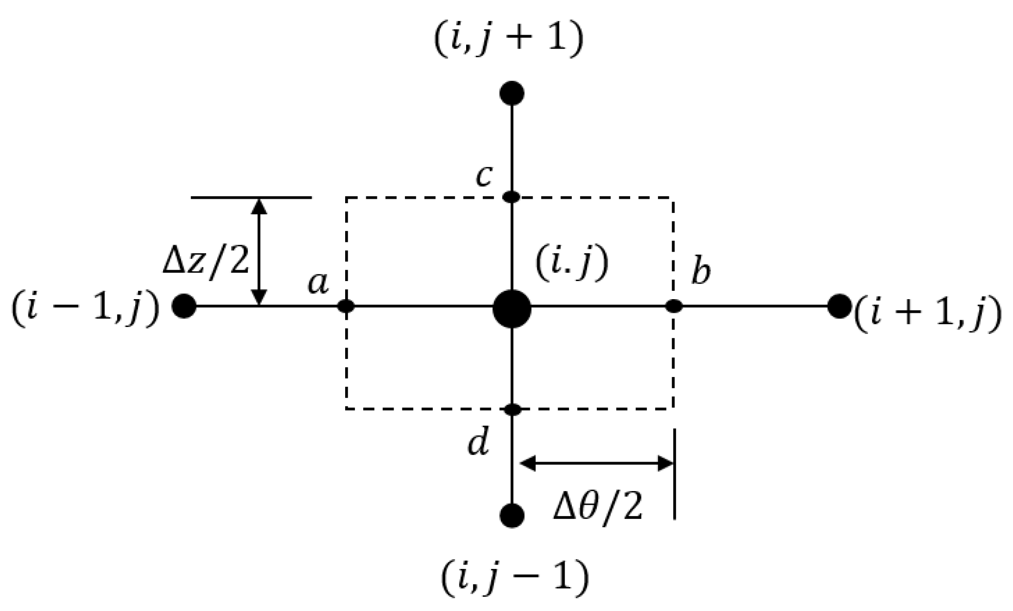
The analytic solution of the hydrodynamic problem in journal bearings is possible for particular cases, where the approximate solutions are obtained. These approximate solutions involve ignoring one of the pressure gradients in the Reynolds equation. The pressure gradient in the circumference direction is ignored in the case of short bearings, and the gradient in the longitudinal direction is ignored in the assumption of long bearings. These assumptions give acceptable results for a certain length-to-diameter ratio of the bearing. However, for finite length bearings where neither of the pressure gradients can be ignored, a numerical solution is required. In this work, the governing equations are solved numerically using the finite difference method. This solution is explained in reference [4]. The solution space is divided to points, where and are the numbers of points in the circumferential and longitudinal direction of the bearing, respectively. Part of the solution space is shown in Figure 3 where point and its surrounding four mesh points are illustrated.
By using the central difference to discretize the pressure gradient as well as the variation of the film thickness in the circumferential direction, it gives us,
The film thickness at the boundaries of the control volume that shown in Figure 3 is used as an average value which can be given by:
Similarly, the gradient in the z direction is discretized as follows:
By substituting Equations (10)–(20) into Equation (2), the pressure at point can be given by:
where: , , , , and are the mesh steps.
The oil film thickness in terms of the position is,
2.5. Solution Procedure
Equation (21) is solved at all points on the solution domain except for the boundaries where the pressure values are set to zero. This step requires a first assumption of the pressure field over this solution domain. The new calculated pressure values are then used as the input values to calculate another pressure field using Equation (21). The pressure distribution in the solution space is obtained iteratively by using a successive over relaxation method to reduce the required number of iterations. The relaxation factor that is used in this case is with there being an optimum value of 1.93. The calculated pressure ( that is based on Equation (11) is updated using the following equation:
where is the pressure value from the previous iteration at the node.
It is worth mentioning that the overall convergence of the solution requires the convergence of the pressure distribution which is given by in addition to the convergence of the load which is explained below.
After the convergence of the solution is achieved, the pressure values are available at all positions in the solution domain. Therefore, the bearing forces in the radial and tangential forces can be easily calculated numerically, using the following discrete forms in order to calculated the total load :
The calculated load is compared with the input load to achieve an accuracy limit that is relative to the input load. If the calculated load is not within this tolerance limit, then the eccentricity ratio is continuously updated until the load convergence is obtained.
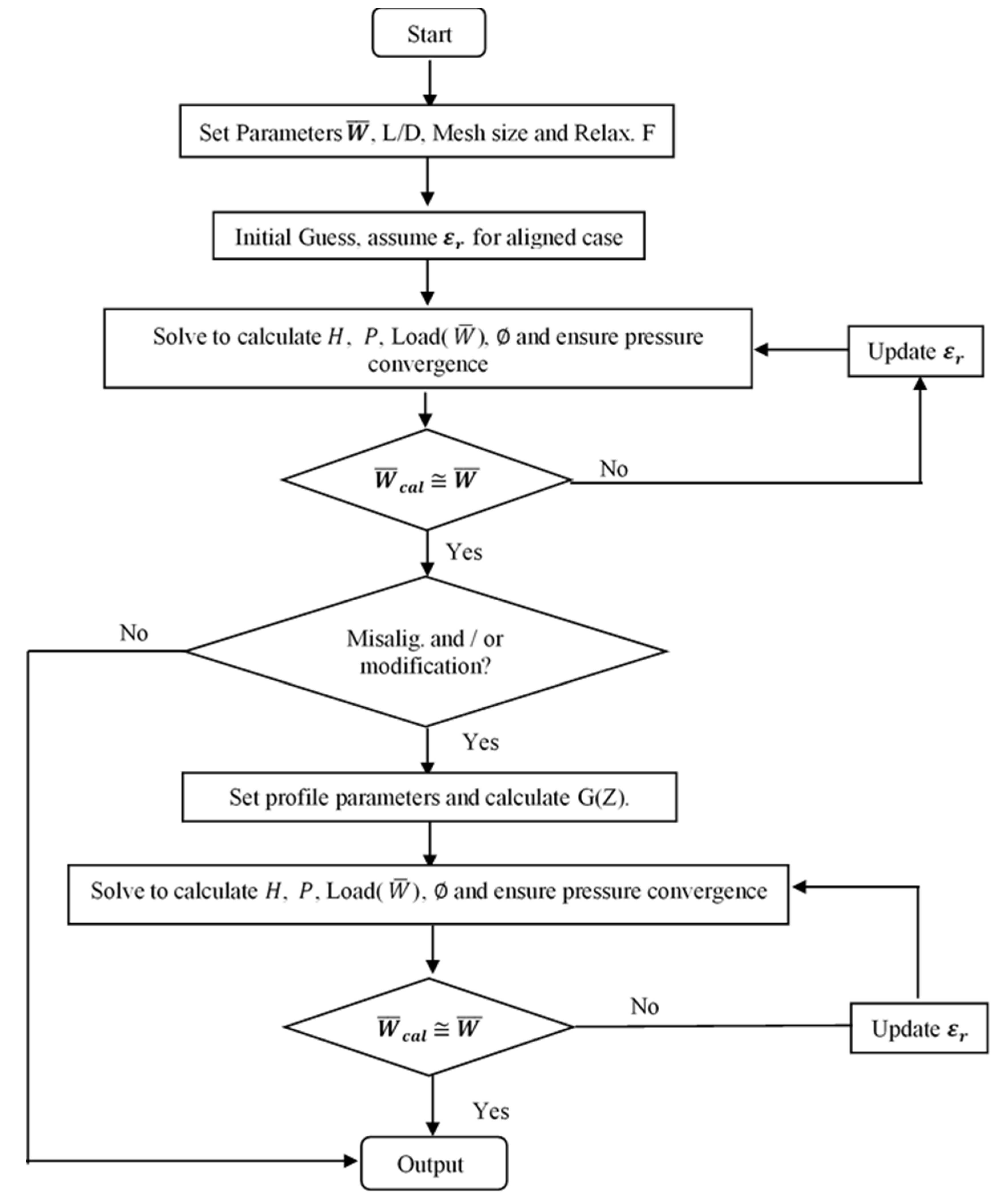
Equations (5)–(8) are also easily discretized and combined with Equation (10) to obtain the total gap between the surfaces at any and node. The Reynolds boundary conditions are used in the solution scheme using an iterative procedure to identify the cavitation zone where and are satisfied at the limit of this zone. It is worth mentioning that the iterations for the misaligned and modified design cases (under overrelaxed solution) are continued until the results converge to the same load in all of the cases. This load corresponds to an eccentricity ratio of 0.6 in the aligned case. A flow chart for the solution scheme is shown in Figure 4.
3. Results and Discussions
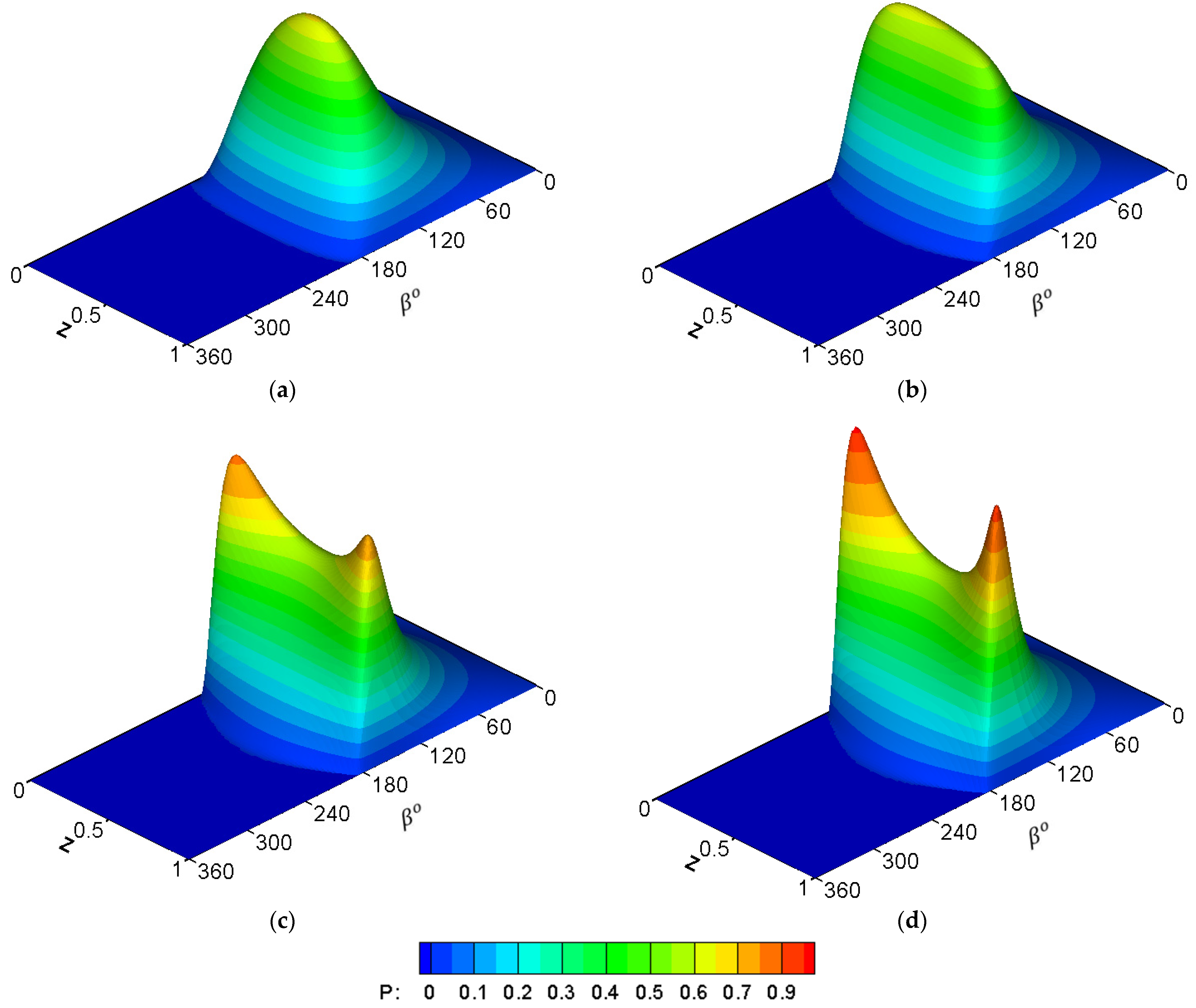
The numerical solution is first performed to examine the required mesh size in both directions that is sufficient enough to obtain independent results on the number of nodes in the solution space. The effect of misalignment on the pressure distribution is shown in Figure 5 for a finite length bearing where . Figure 5a shows the case when , which represents a perfectly aligned bearing. It can be seen how the pressure distribution is uniform and symmetric about the line (half of the bearing length). Figure 5b–d shows the results for the cases , and .58, respectively. The case of is chosen as the intermediate step between the perfectly aligned bearing and the extreme cases of and . The film thickness becomes extremely thin in the last two cases, and it is explained below, the maximum pressure values correspond to each case.
The influences of bearing edge chamfering on the pressure distributions are shown in Figure 6. The result of the misaligned case (without modification) that is presented in previous figure is repeated here for the purpose of comparison, as shown in Figure 6a, where . Figure 6b–d shows the effect of the modification on the pressure distribution where , and , respectively. These values are selected to be presented in this figure after implementing a wide range of modification parameters and in the solution scheme.
It can be seen from this figure that the modification returns to some degree the symmetrical pressure distribution despite the presence of a misalignment. This outcome is expected to have significant effects on the dynamic behavior of the system, particularly when it is under dynamic load such as impact load and position perturbation, which will be addressed comprehensibly in future work.
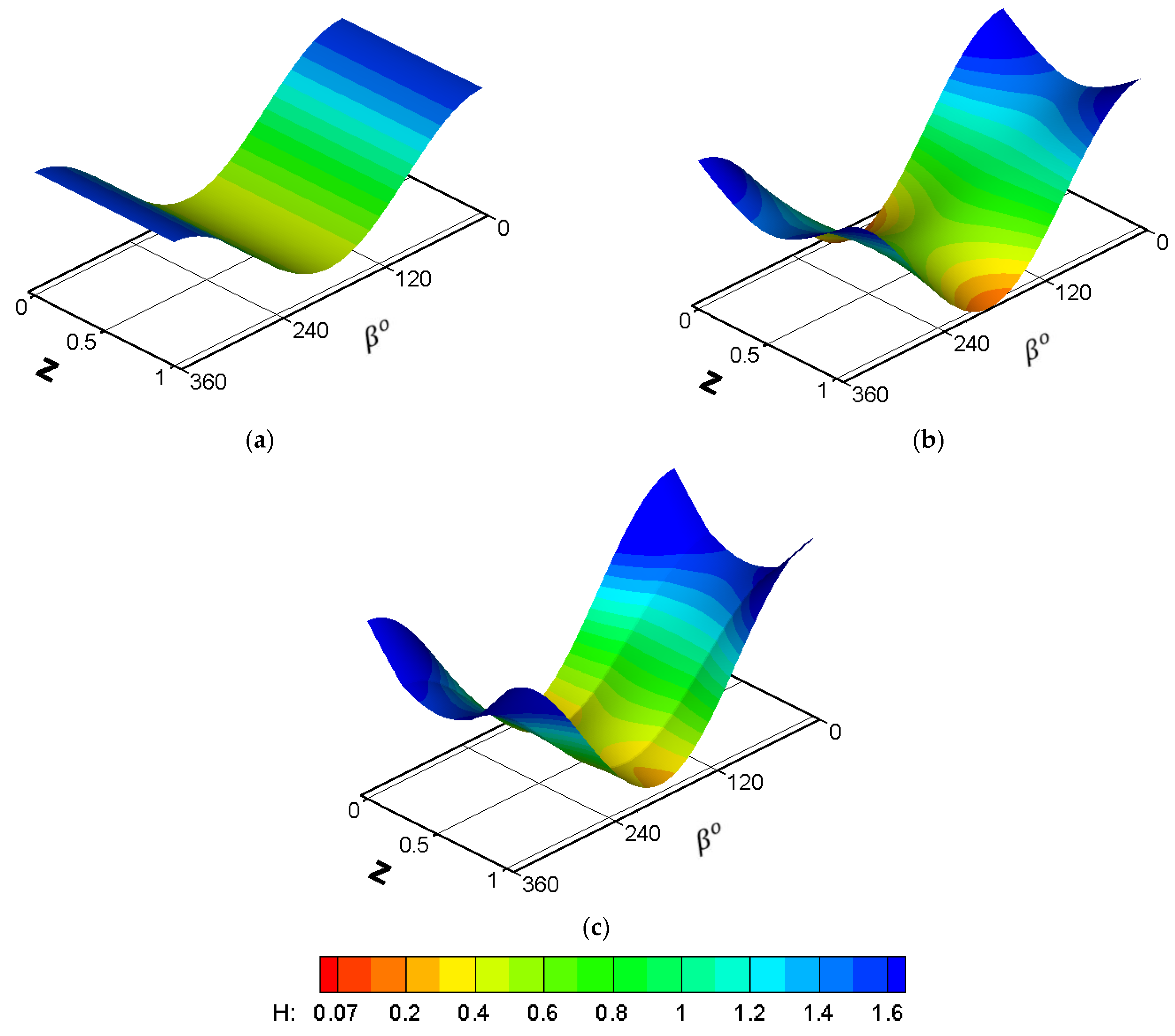
The corresponding film thickness distributions are shown in Figure 7. Figure 7a shows the case of the aligned bearing, while Figure 7b shows the results of the misaligned case where . Figure 7c illustrates the effect of modification on the film thickness of a misaligned bearing where and . These figures explain how the misalignment disturbs the perfectly extruded shape of film thickness along the bearing’s length which results in a reduction in the film thickness and a concentration of the pressure spikes that are close to the film thinning position which is related to the misalignment.
Figure 8 shows a more detailed comparison for the previous results at the section of maximum pressure in the circumferential direction. Figure 8a shows the results of the pressure variation, whereas Figure 8b shows the corresponding results about the film thickness for three cases of a perfectly aligned bearing, a misaligned bearing and a modified misaligned bearing (where ). It is clear from these figures that removing material from the bearing’s inner surface at the edges brings back the shape of both the pressure and film thickness at a level that is very close to the normal case of an aligned bearing at the position of maximum pressure.
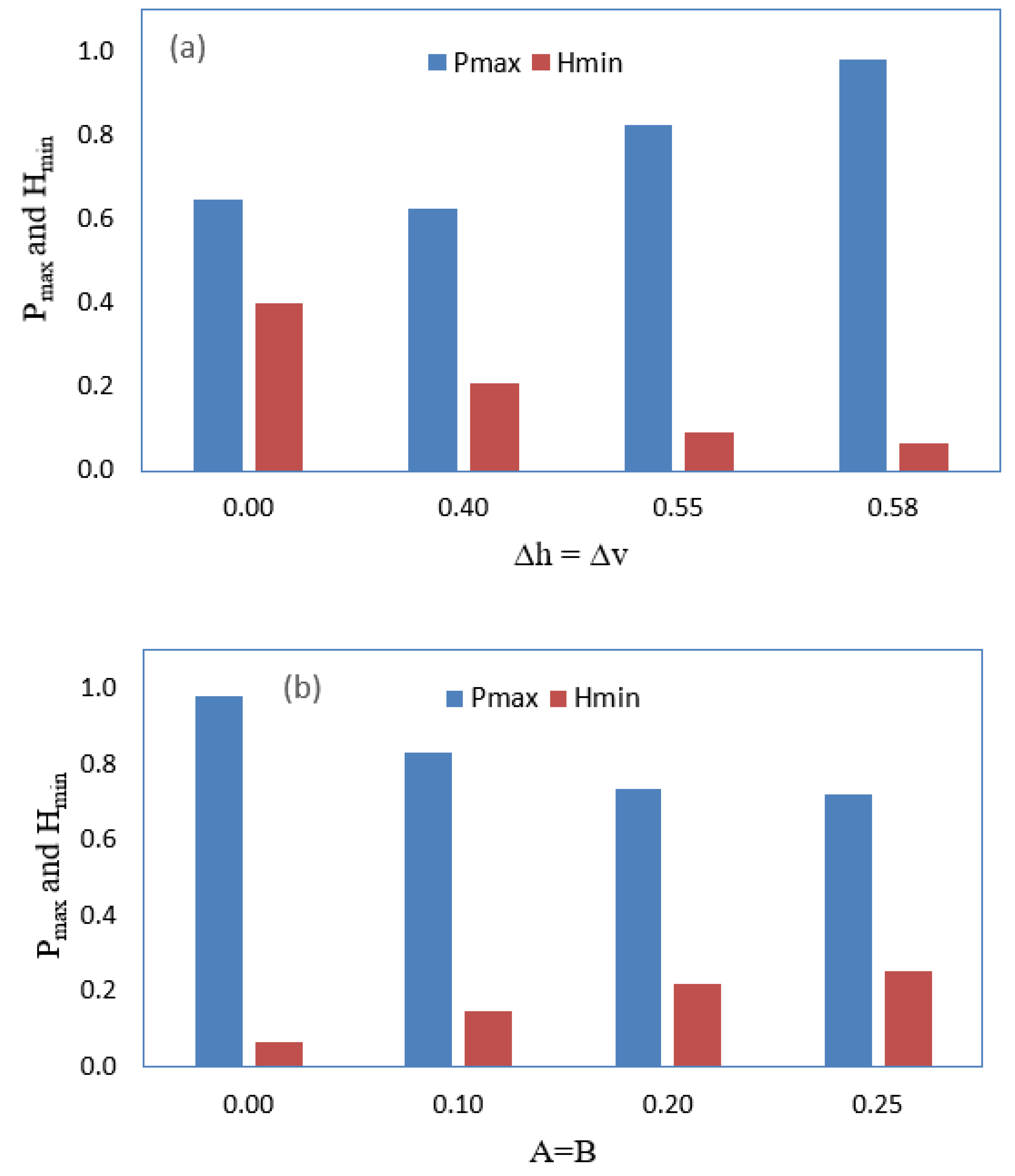
The values of and for the cases that are shown in Figure 5 and Figure 6 are shown in Figure 9a,b, respectively. The maximum pressure increases by 51.63 %, in comparison with the aligned case when and the corresponding film thickness reduces by 83.5%. The bearing chamfering reduces the by 26.38% and increases the to be 0.254, which was 0.066 (an increase of 284.85%) when for the misaligned bearing. This important outcome is expected to have positive consequences on the bearing life through the limitation of the occurrence of partial contact between the asperities (mixed regime) of the shaft and the journal bushing when a very thin layer of oil is interposed in the resulting wedge.
More details about the effect of the modification parameters on the maximum pressure and the minimum film thickness of the misaligned bearings are shown in Table 1. In this table, two extreme misalignment cases that were under wide range of chamfer parameters are investigated. The misalignments in these cases have the following values: and . On the other hand, the modification parameters are (Unmodified bearings), , , and . It can be seen that in both cases, the modification reduces the maximum pressure values and increases the minimum film thickness when the chamfer parameters are less than 0.3. When , the minimum film thickness continues to increase but, on the other hand, the maximum pressure value also increases. This can be attributed to the fact that as the parameter increases (modification parameter in the radial direction), the modification part of the bearing will be less involved in supporting the load. This can be explained in other words; that the pressure will generate over a smaller part of the modified portion of the bearing. Despite that the pressure values are slightly increased when , higher values for the chamfer parameters are not recommended.
Table 2 shows the results of the coefficient of friction for three cases which are the perfectly aligned shaft and bush , the misaligned shaft ( and the modified bush under misalignment (. It is worth mentioning that the coefficient of friction is calculated for a wide range of cases where different values for both the misalignment and the chamfering parameters were considered and the values that are shown in this table are the most important ones for the purpose of comparison. In general, a misalignment has no significant effect on the friction coefficient unless it causes an essential reduction in the oil film thickness. The values that are shown in this table provide a clear picture for the effect of chamfer for the cases that are discussed in the previous figures, where the film thickness is reduced significantly due to the presence of a misalignment. It can be seen that in the first case, the coefficient of friction is 2.218 and in the second case, the misalignment increases the friction coefficient by 14.56%.
On the other hand, chamfering the bush edges for the misaligned case reduces the coefficient of friction by 9.76%, in comparison to that which is achieved with the misaligned case. However, as the misalignment reduces, the thickness of the lubricant layer that is close to the bush edges increases. The surface roughness of the shaft and the bush will certainly have its contribution to the friction between the two surfaces. In such case, the coefficient of friction in the misaligned case is clearly more than the calculated value is as based on the approach that adopted in this work. Therefore, a more realistic analysis is required to consider the surface features that are at least over the region where the film thickness is relatively thin. Such a solution requires an elastohydrodynamic analysis of the contact problem in order to incorporate the deformation of the rough surfaces. Nevertheless, chamfering the bush edges increases the minimum film thickness significantly, as illustrated previously (see Figure 9). This is highly expected to minimize the surface features’ effects on the characteristics of this contact problem. However, the elastohydrodynamic analysis of the contact problem of the journal bearing while considering the surface features that are under misalignment as well as bush chamfering will be studied by the authors in future works.
4. Conclusions
In this work, the effects of chamfering the bearing inner surface on the pressure and film thickness distributions are presented in detail. A 3D misalignment model is incorporated in the analysis scheme where a numerical solution is used to solve the problem of the finite length journal bearing. The solution procedure involves the use of the Reynolds boundary conditions, where the limit of the cavitation zone is determined iteratively. the results showed that such a design overcomes the problem of the thinning of the lubricant layer that is due to misalignment by increasing the film thickness significantly (almost three times) and helping to reduce the pressure spike that result due to misalignment by 26.38%. The coefficient of friction which is one of the most important characteristics of this type of bearing is also reduced by 9.76% due to introducing the chamfering of the bush edges in comparison with the misaligned case. Another important outcome has been found is the reduction of non-symmetry in the 3D pressure distribution which is expected to have marked influence on the dynamic response of the rotor-bearing system through its impact on the dynamic coefficients.
Author Contributions
H.U.J.: Numerical methodology and writing; H.S.S.: Numerical methodology; A.S.: investigation and writing—review and editing; Z.A.A.-D.: Numerical methodology visualization; M.J.J.: writing—review and editing; A.M.A.: writing—review and editing; O.I.A.: methodology and writing—review and editing; All authors have read and agreed to the published version of the manuscript.
Funding
This research received no external funding.
Institutional Review Board Statement
Not applicable.
Informed Consent Statement
Not applicable.
Data Availability Statement
The study did not report any data.
Conflicts of Interest
The authors declare no conflict of interest.
Nomenclature
| Symbol | Description | Units |
| Design parameters | m | |
| A, B | Dimensionless design parameters | - |
| Clearance | m | |
| Eccentricity of journal | m | |
| Oil film thickness | m | |
| Dimensionless film thickness, | - | |
| Dimensionless Minimum Oil film thickness | - | |
| Bearing length | m | |
| Dimensionless oil film pressure, | - | |
| Bearing radius | m | |
| Velocity | m/s | |
| Mean velocity | m/s | |
| Axial coordinate, | m | |
| Dimensionless coordinate, | - | |
| degree | ||
| Attitude angle | degree | |
| General description of misalignment ( or) | m | |
| Horizontal misalignment | m | |
| Vertical misalignment | m | |
| General dimensionless description of misalignment ( | - | |
| Dimensionless horizontal misalignment | - | |
| Dimensionless horizontal misalignment at the bearing edge | - | |
| Dimensionless vertical misalignment | - | |
| Dimensionless vertical misalignment at the bearing edge | - | |
| Eccentricity Ratio, | - | |
| Lubrication viscosity | Pa·s | |
| Mass density of oil | kg/ | |
| Angle in the circumferential direction | degree | |
| ω | Journal Angular velocity, | rad/s |
| Step in the circumferential direction | degree | |
| Step in the longitudinal direction | - |
References
- Omidreza, E.; Zissimos, P. Mourelatos, Nickolas Vlahopoulos & Kumar Vaidyanathan Calculation of Journal Bearing Dynamic Characteristics Including Journal Misalignment and Bearing Structural Deformation©. Tribol. Trans. 2004, 47, 94–102. [Google Scholar] [CrossRef]
- Sun, J.; Gui, C.L. Hydrodynamic lubrication analysis of journal bearing considering misalignment caused by shaft deformation. Tribol. Int. 2004, 37, 841–848. [Google Scholar] [CrossRef]
- Jang, J.; Khonsari, M. On the characteristics of misaligned journal bearings. Lubricants 2015, 3, 27–53. [Google Scholar] [CrossRef]
- Jamali, H.U.; Al-Hamood, A. A New Method for the Analysis of Misaligned. J. Bear. Tribol. Ind. 2018, 40, 213–224. [Google Scholar] [CrossRef]
- Song, X.; Wu, W.; Yuan, S. Mixed-lubrication analysis of misaligned journal bearing considering turbulence and cavitation. AIP Adv. 2022, 12, 015213. [Google Scholar] [CrossRef]
- Xin, Q. Diesel Engine System Design; Woodhead Publishing Limited: Sawston, UK, 2011; Chapter 10; pp. 651–758. [Google Scholar] [CrossRef]
- Muskat, M.; Morgan, F. Studies in lubrication V. the theory of the thick film lubrication of flooded journal bearings and bearings with circumferential grooves. J. Appl. Phys. 1939, 10, 398–407. [Google Scholar] [CrossRef]
- Dufrane, K.F.; Kannel, J.W.; McCloskey, T.H. Wear of steam turbine journal bearings at low operating speeds. J. Lubr. Technol. 1983, 105, 313–317. [Google Scholar] [CrossRef]
- Unlu, B.S.; Durmus, H.; Mericc, C.; Atik, E. Determination of friction coefficient at journal bearings by experimental and by means of artificial neural networks method. Math. Comput. Appl. 2004, 9, 399–408. [Google Scholar]
- Goenka, P.K. Dynamically loaded journal bearings: Finite element method analysis. J. Tribol. Trans. ASME 1984, 106, 429–439. [Google Scholar] [CrossRef]
- Nikolakopoulos, P.G.; Papadopoulos, C.A. Non-linearities in misaligned journal bearings. Tribol. Int. 1994, 27, 243–257. [Google Scholar] [CrossRef]
- Bouyer, J.; Fillon, M. An experimental analysis of misalignment effects on hydrodynamic plain journal bearing performances. J. Tribol. 2002, 124, 313–319. [Google Scholar] [CrossRef]
- Boedo, S.; Booker, J.F. Classical bearing misalignment and edge loading: A numerical study of limiting cases. J. Tribol. 2004, 126, 535–541. [Google Scholar] [CrossRef]
- Sun, J.; Gui, C.; Li, Z. An experimental study of journal bearing lubrication effected by journal misalignment as a result of shaft deformation under load. J. Tribol. 2005, 127, 813–819. [Google Scholar] [CrossRef]
- Padelis, G. Nikolakopoulos, C.; Papadopoulos, A. A study of friction in worn misaligned journal bearings under severe hydrodynamic lubrication. Tribol. Int. 2008, 41, 461–472. [Google Scholar] [CrossRef]
- Nacy, S.M. Effect of Chamfering on Side-Leakage Flow Rate of Journal Bearings. Wear 1997, 212, 95–102. [Google Scholar] [CrossRef]
- Fillon, M.; Bouyer, J. Thermohydrodynamic Analysis of a Worn Plain Journal Bearing. Tribol. Int. 2004, 37, 129–136. [Google Scholar] [CrossRef]
- Strzelecki, S. Operating Characteristics of Heavy Loaded Cylindrical Journal Bearing with Variable Axial Profile. Mater. Res. 2005, 8, 481–486. [Google Scholar] [CrossRef]
- Chasalevris, A.; Dohnal, F. Enhancing Stability of Industrial Turbines Using Adjustable Partial Arc Bearings. J. Phys. 2016, 744, 012152. [Google Scholar] [CrossRef]
- Ren, P.; Zuo, Z.; Huang, W. Effects of axial profile on the main bearing performance of internal combustion engine and its optimization using multiobjective optimization algorithms. J. Mech. Sci. Technol. 2021, 35, 3519–3531. [Google Scholar] [CrossRef]
- Booker, J.F.; Boedo, S.; Bonneau, D. Conformal elastohydrodynamic lubrication analysis for engine bearing design: A brief review. Proceedings of the Institution of Mechanical Engineers. Part C J. Mech. Eng. Sci. 2010, 224, 2648–2653. [Google Scholar] [CrossRef]
- Allmaier, H.; Offner, G. Current Challenges and Frontiers for the EHD Simulation of Journal Bearings: A Review; SAE Technical Paper 2016-01-1856; SAE International: Warrendale, PA, USA, 2016. [Google Scholar] [CrossRef]
- Krishnkant, S.; Satish, C.; Sharma, N.R. Misalignment and Surface Irregularities Effect in MR Fluid Journal Bearing. Int. J. Mech. Sci. 2022, 221, 107196. [Google Scholar] [CrossRef]
- Guo, J.; Xiang, G.; Wang, J.; Song, Y.; Cai, J.; Dai, H. On the dynamic wear behavior of misaligned journal bearing with profile modification under mixed lubrication. Surface Topogr. Metrol. Prop. 2022, 10, 025026. [Google Scholar] [CrossRef]
- Jameel, A.; Ali, A.; Mohammad, T. Dynamic Stability Analysis and Critical Speed of Rotor supported by a Worn Fluid film Journal Bearings. J. Eng. 2016, 22, 148–167. [Google Scholar]
- Shamal, S.J.; Al-Ansari, L.S.; Alhusseny, A.N.M.; Nasser, A.G. Roughness Effect on Thermo-Elasto-Hydrodynamic Performance of a 170ᵒ-Arc Partial Journal Bearing. J. Eng. 2021, 27, 16–34. [Google Scholar] [CrossRef]
- Sattar, M.A.; Yousif, A.E. The Effect of Additives on The Performance of HydrostaticThrust Bearings. Al-Khwarizmi Eng. J. 2008, 4, 57–70. [Google Scholar]
- Zhou, W.; Wang, Y.; Wu, G.; Gao, B.; Zhang, W. Research on the lubricated characteristics of journal bearing based on finite element method and mixed method. Ain Shams Eng. J. 2022, 13, 101638. [Google Scholar] [CrossRef]
- Sayed, H.; El-Sayed, T.A. A Novel Method to Evaluate the Journal Bearing Forces with Application to Flexible Rotor Model. Tribol. Int. 2022, 173, 107593. [Google Scholar] [CrossRef]
- Lund, J.W.; Thomsen, K.K. A Calculation Method and Data for the Dynamic Coefficients of Oil-Lubricated Journal Bearings, Topics in Fluid Film Bearing and Rotor Bearing System Design and Optimization. ASME 1978, 1–28. [Google Scholar]
Figure 1.
Schematic drawing of the journal-bearing. (a) Side view of aligned bearing, (b) 3D representation and (c) misalignment model used in this work.
Figure 1.
Schematic drawing of the journal-bearing. (a) Side view of aligned bearing, (b) 3D representation and (c) misalignment model used in this work.
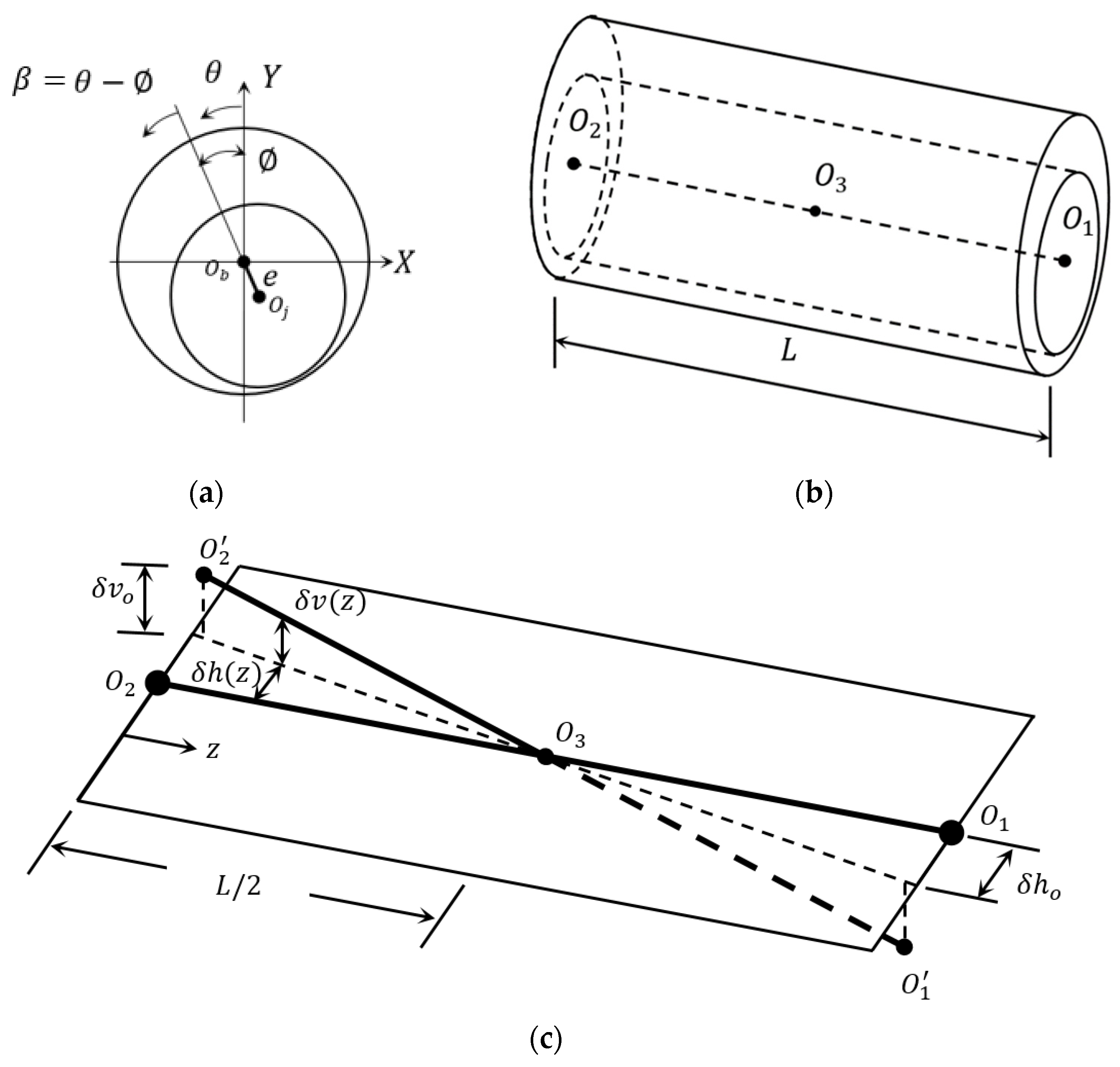
Figure 2.
Bearing with modified edges. (a) 3D full bearing, (b) 3D section and (c) Schematic drawing of the bearing after removing material from the inner surface.
Figure 2.
Bearing with modified edges. (a) 3D full bearing, (b) 3D section and (c) Schematic drawing of the bearing after removing material from the inner surface.
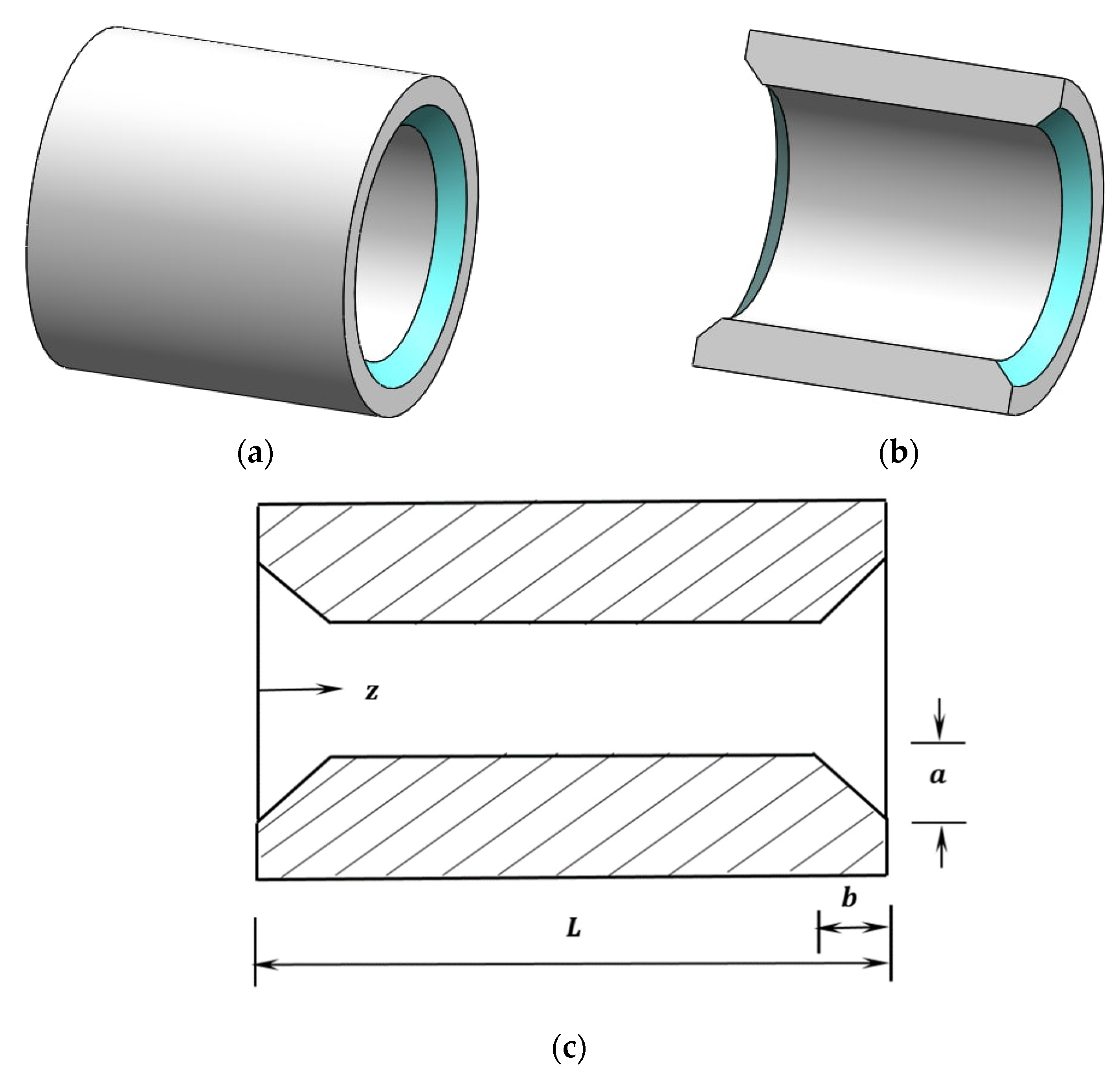
Figure 3.
Part of solution domain.

Figure 4.
Flow chart for the solution procedure.

Figure 5.
Effect of misalignment on dimensionless pressure distribution (L/D = 1.25). (a): Aligned, (b): , (c): and (d): . .
Figure 5.
Effect of misalignment on dimensionless pressure distribution (L/D = 1.25). (a): Aligned, (b): , (c): and (d): . .

Figure 6.
Effect of linear modification on dimensionless pressure distribution (L/D = 1.25) when (a): Without modification, (b): , (c): and (d): .
Figure 6.
Effect of linear modification on dimensionless pressure distribution (L/D = 1.25) when (a): Without modification, (b): , (c): and (d): .
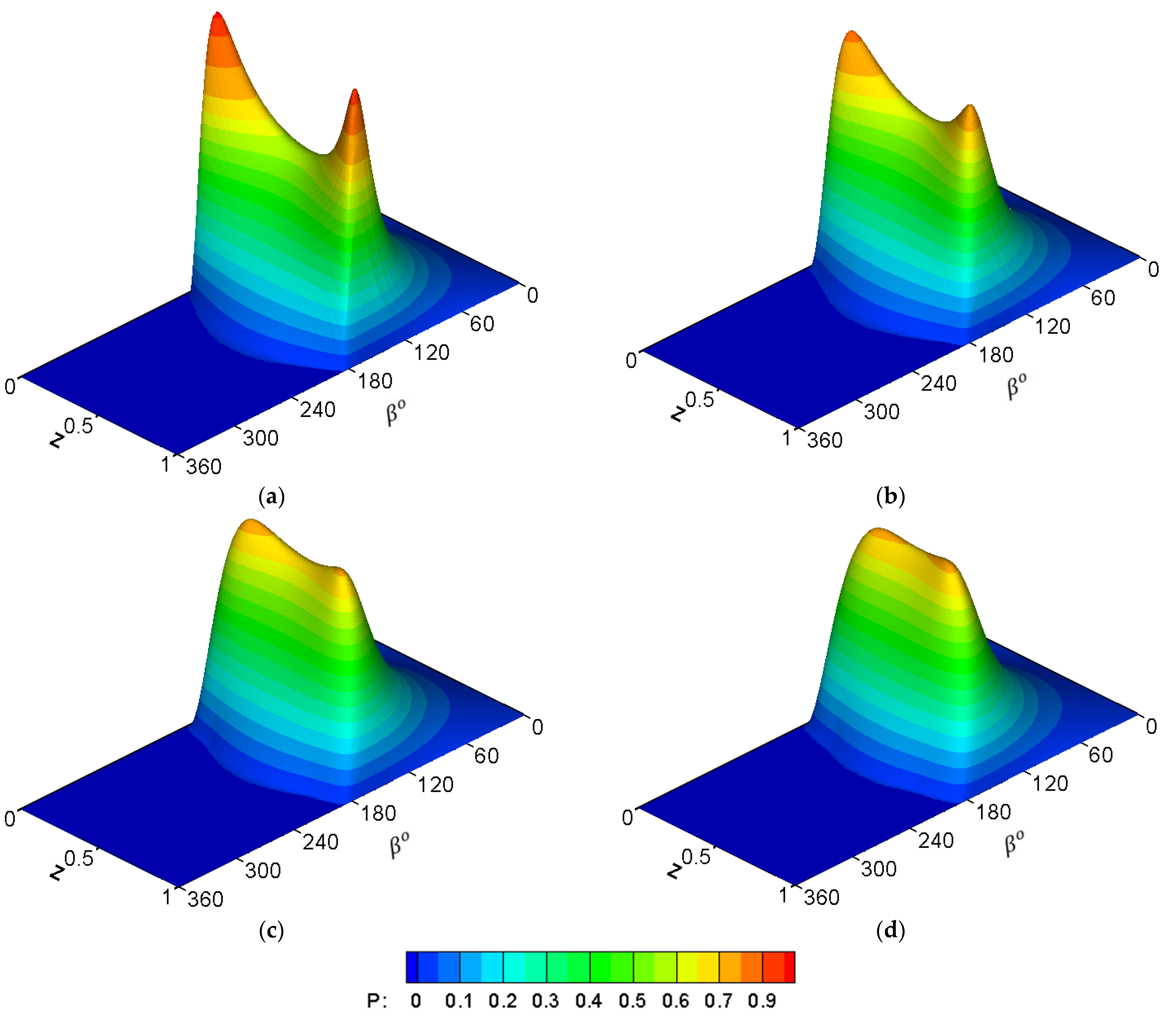
Figure 7.
Dimensionless film thickness (L/D = 1.25). (a): Aligned (, (b): misaligned and (c): modified bearing ( and ).
Figure 7.
Dimensionless film thickness (L/D = 1.25). (a): Aligned (, (b): misaligned and (c): modified bearing ( and ).

Figure 8.
Effect of misalignment and profile modification on (a): pressure variation and (b): film thickness at the section of maximum pressure.
Figure 8.
Effect of misalignment and profile modification on (a): pressure variation and (b): film thickness at the section of maximum pressure.
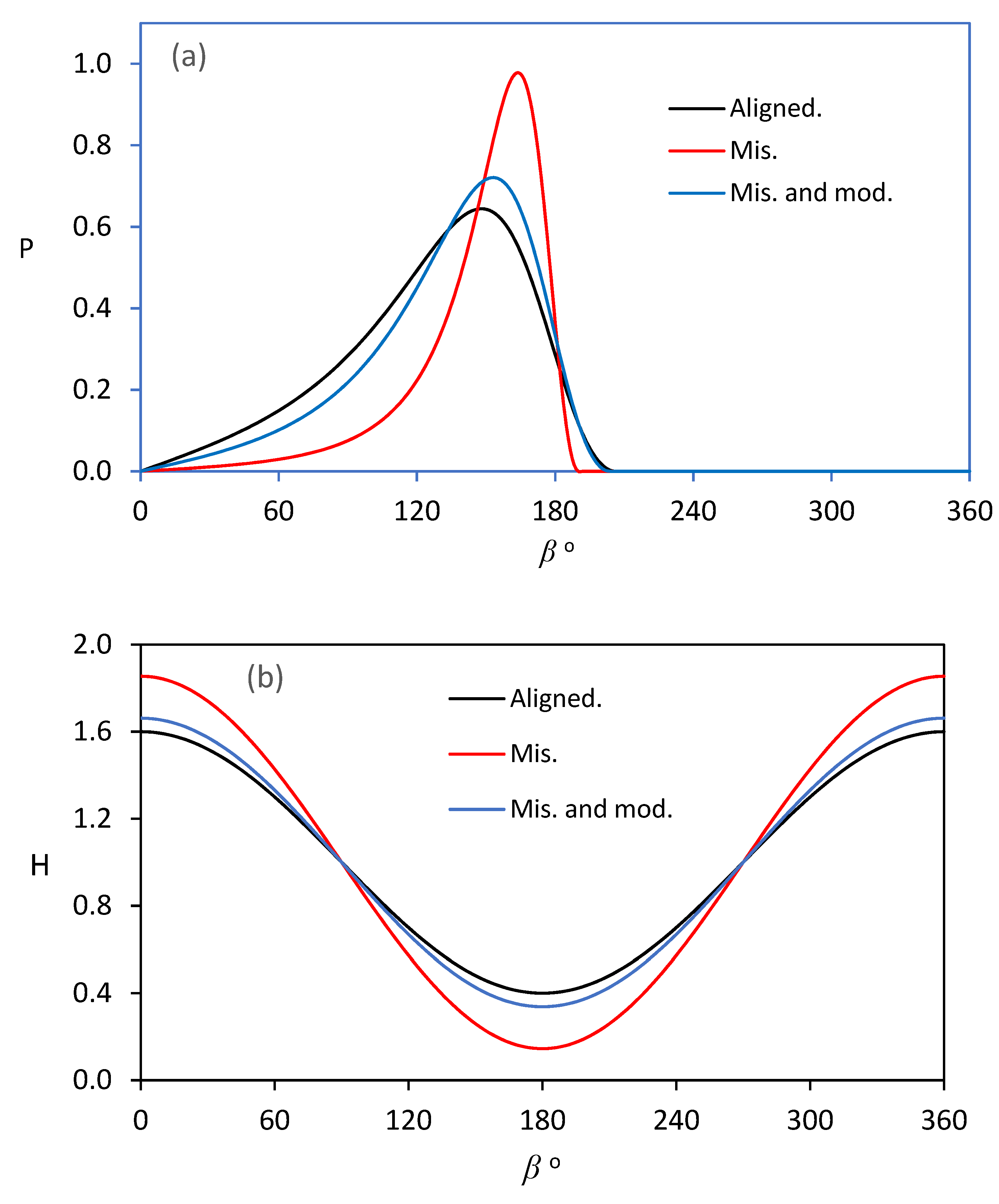
Figure 9.
Dimensionless maximum pressure and minimum film thickness for (a): unmodified bearing with different misalignment values and (b) modified misaligned bearing when .
Figure 9.
Dimensionless maximum pressure and minimum film thickness for (a): unmodified bearing with different misalignment values and (b) modified misaligned bearing when .


Table 1.
Effect of modification parameters on maximum pressure and minimum film thickness of misaligned bearings (Dimensionless).
Table 1.
Effect of modification parameters on maximum pressure and minimum film thickness of misaligned bearings (Dimensionless).
| Case | Unmodified Bearings | Modified Bearings | ||||||||
|---|---|---|---|---|---|---|---|---|---|---|
| 0.824 | 0.091 | 0.751 | 0.173 | 0.716 | 0.268 | 0.714 | 0.280 | 0.756 | 0.306 | |
| 0.978 | 0.066 | 0.830 | 0.145 | 0.733 | 0.218 | 0.720 | 0.254 | 0.749 | 0.278 | |
Table 2.
The values for the coefficient of friction calculations for different cases.
| Case |
Aligned |
Misaligned |
Misaligned, Modified Edges |
|---|---|---|---|
| 2.218 | 2.535 | 2.288 |
Publisher’s Note: MDPI stays neutral with regard to jurisdictional claims in published maps and institutional affiliations. |
© 2022 by the authors. Licensee MDPI, Basel, Switzerland. This article is an open access article distributed under the terms and conditions of the Creative Commons Attribution (CC BY) license (https://creativecommons.org/licenses/by/4.0/).
Share and Cite
MDPI and ACS Style
Jamali, H.U.; Sultan, H.S.; Senatore, A.; Al-Dujaili, Z.A.; Jweeg, M.J.; Abed, A.M.; Abdullah, O.I. Minimizing Misalignment Effects in Finite Length Journal Bearings. Designs 2022, 6, 85. https://doi.org/10.3390/designs6050085
AMA Style
Jamali HU, Sultan HS, Senatore A, Al-Dujaili ZA, Jweeg MJ, Abed AM, Abdullah OI. Minimizing Misalignment Effects in Finite Length Journal Bearings. Designs. 2022; 6(5):85. https://doi.org/10.3390/designs6050085
Chicago/Turabian StyleJamali, Hazim U., Hakim S. Sultan, Adolfo Senatore, Zahraa A. Al-Dujaili, Muhsin Jaber Jweeg, Azher M. Abed, and Oday I. Abdullah. 2022. "Minimizing Misalignment Effects in Finite Length Journal Bearings" Designs 6, no. 5: 85. https://doi.org/10.3390/designs6050085