A Design Synthesis Method for Robust Controllers of Active Vehicle Suspensions ^†

Abstract

This paper presents a design synthesis method for robust controllers of active vehicle suspensions (AVSs). Various control techniques have been applied to the design of AVSs for enhancing ride comfort and handling performance of ground vehicles. However, most of these model-based controller designs show poor robustness when the vehicle models are not accurate and operating conditions vary. To address the poor robustness problem of AVSs, a new controller is designed using the $H_{\infty }$ loop-shaping control technique. The controller targets robustness issues on vehicle models with parametric uncertainties and unmodelled dynamics. To facilitate the robust controller design, a design synthesis method is proposed: the $H_{\infty }$ loop-shaping controller design is formulated as a multi-objective optimization problem, the weighting functions’ parameters of the controller are treated as design variables, the expensive computing loads are handled by a parallel computing technique, and the solution of the optimization problem is the desired robust AVS controller. Simulation results demonstrate the benefits of the proposed AVS design.

1. Introduction

With given elastic and damping features, passive vehicle suspensions show poor ride quality when traveling in severe operating conditions, e.g., low frequency bumps, pit holes, and high frequency road irregularities [1]. In contrast, active vehicle suspensions (AVSs) adjust these properties to external disturbances in a broadband frequency range for improving ride comfort and handling performance [2]. Semi-active suspensions provide a compromised solution between passive and active suspensions in terms of performance and cost (i.e., energy consumption) [3,4].

The linear quadratic Gaussian (LQG) and linear quadratic regular (LQR) techniques have been used in the design of AVSs [5,6,7,8]. In these LQG/LQR-based AVS designs, forward speed, payload, center of gravity (CG) position, and other system parameters are generally assumed as constants. It is demonstrated that these LQG/LQR-based controllers exhibit poor robustness to operating condition variations, parametric uncertainties, unmodelled dynamics, and external disturbances [9,10].

To address the poor robustness of these LQG/LQR-based controllers, robust control techniques, e.g., $H_{\infty }$ [11] and sliding-mode control [12,13,14,15], have been applied to the design of active vehicle safety systems. Robustness is a fundamental requirement for a controller design due to the differences between the dynamic model utilized for devising the controller and the actual physical system [16]. Attempts have been made to compare the robust control characteristics of $H_{\infty }$/$\mu$-synthesis control and sliding-mode control for different active vehicle safety systems [17,18]. The $H_{\infty }$ control technique has been successfully used for addressing robustness problems on models with external disturbances and parametric uncertainties [19,20,21].

However, due to the complex conflicting suspension design requirements on ride quality, suspension working space, and dynamic tire loading [22], the $H_{\infty }$-based AVS controllers reported in the literature have not adequately addressed the trade-off design problem [23]. Moreover, one of the challenges in the $H_{\infty }$ controller design is parameters’ tuning for weighting functions [16]. The weighting functions pose significant impacts on the performance and robustness of the respective $H_{\infty }$ controller design. Conventionally, the parameters of weighting functions are tuned by the trial and error approach [24]. This parameter tuning process is time-consuming and tedious.

To tackle the aforementioned problems associated with the $H_{\infty }$-based AVS controller designs, this paper proposes a design synthesis method for the $H_{\infty }$ controller of AVSs. A robust $H_{\infty }$ loop-shaping controller (LSC) is designed for an AVS of a vehicle represented by a quarter-car model. In the controller design, vehicle parametric uncertainties are considered. The frequency weighting functions are specified by selecting optimal values for the parameters through solving a multi-objective optimization problem with the expensive computation loads handled by a parallel computing technique provided in Matlab. Numerical simulation is performed to demonstrate the effectiveness of the proposed design synthesis method.

The remainder of the paper is organized as follows. Section 2 introduces the vehicle model. Section 3 formulates the $H_{\infty }$ controller design problem. The proposed design synthesis method is described in Section 4. Section 5 presents selected simulation results. Conclusions are drawn in Section 6.

2. Vehicle Model

To investigate the ride comfort of road vehicles, various dynamic models have been generated and used. In particular, to study the ride comfort and handling characteristics of a passenger car, a 7 degrees of freedom (DOF) ‘full-car’ model was proposed [4,25]. In this model, the bounce, roll, and pitch of the vehicle body, as well as the bounce of the four wheels are considered. Assuming that the car travels on a good road and the difference between right and left wheel track undulations can be ignored, we may neglect the roll motion of the vehicle body, and the 7-DOF model may be reduced to a 4-DOF ‘half-car’ model [25]. In the 4-DOF model, the bounce and pitch of the vehicle body, as well as the bounce of the front and rear wheels are taken into consideration. For the half-car model, it is assumed that the sprung mass, i.e., the mass of the vehicle body, is distributed at three points, that is, the point of attachment of front suspension to the vehicle body, the CG, and the point of attachment of rear suspension to the vehicle body. Considering the fact that for conventional passenger cars, the sprung mass distribution coefficient is within the range of 0.9 to 1.0 [26], the concentrated mass at the CG of the half-car model is approximately zero, and the motions of the front and rear suspensions of the half-car model are uncoupled. Thus, the 4-DOF half-car model can be further simplified and reduced to a 2-DOF ‘quarter-car’ model, which considers the bounce of the sprung and unsprung mass [15]. Note that the sprung mass distribution coefficient is defined as $\epsilon =\raisebox{1ex}{${\rho }_y^2$}\!\left/ \!\raisebox{-1ex}{$ab$}\right.$, where ${\rho }_y$ denotes the radius of gyration of the half-car sprung mass with respect to the lateral axis (i.e., y axis) of the body fixed coordinate system, $a$ the distance between the CG to the front axle, and $b$ the distance between the CG to the rear axle.

A road vehicle represents a sophisticated vibration system with many degrees of freedom. In general, the vehicle model fidelity increases with the degrees of freedom of the model. However, the analysis burden becomes increasingly heavy while increasing the degrees of freedom. It is rational to simplify the complex vibration system by considering only its major motions. To gain a qualitative insight into the functions of the suspension and, in particular, the effects of the sprung and unsprung mass, spring stiffness, and damping on vehicle vibrations, a linear 2-DOF quarter-car model may be used [26]. With the aforementioned considerations, this study selects the linear 2-DOF quarter-car model to explore the robust controllers for AVSs.

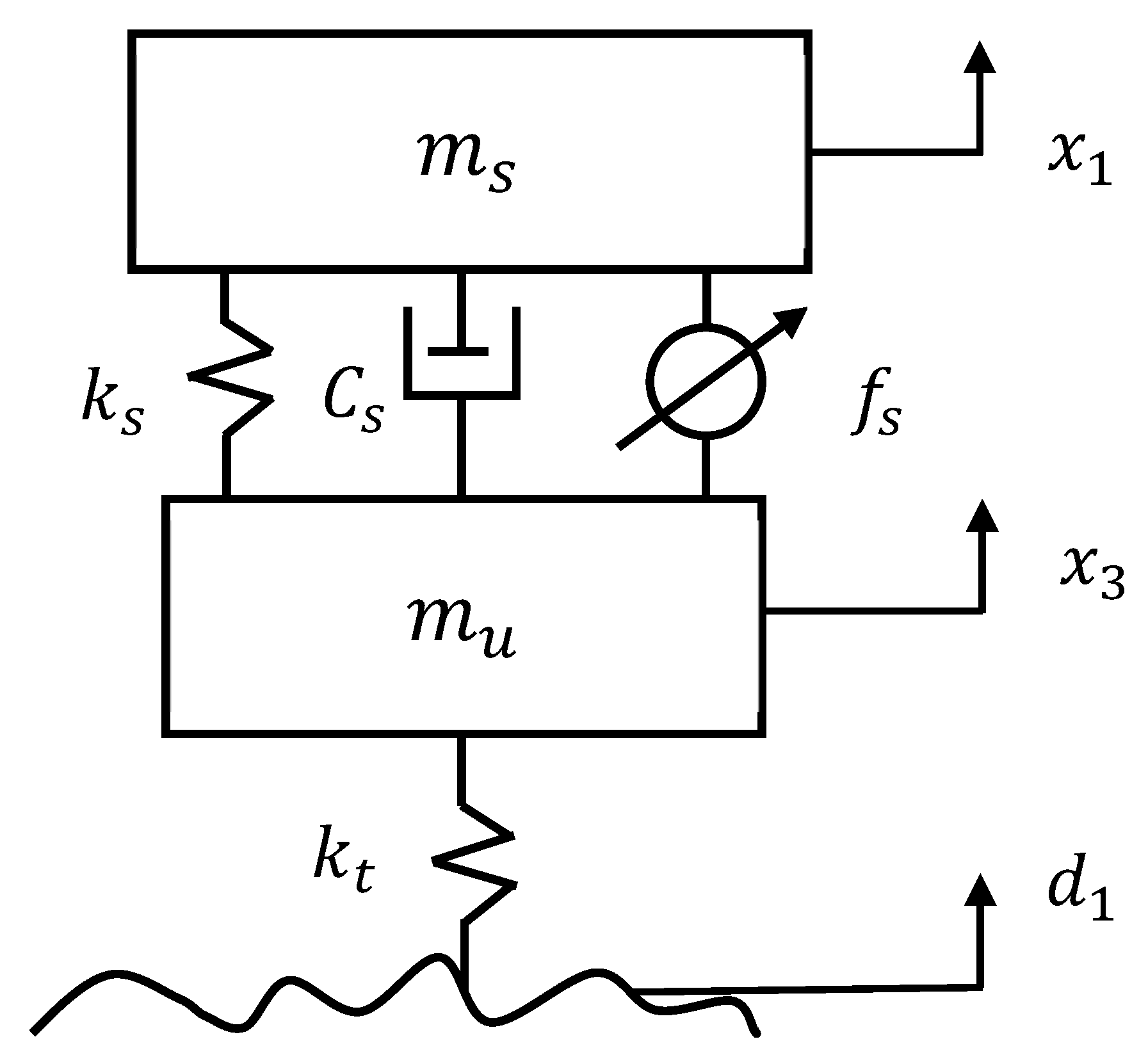
Figure 1 illustrates the linear 2-DOF quarter-car model with an unsprung mass $m_u$, sprung mass $m_s$, tire spring stiffness $k_t$, and a suspension with a linear spring with stiffness $k_s$, as well as a linear damper with damping coefficient $c_s$ [8]. As shown in the figure, $d_1$ denotes the external disturbance due to the road roughness, $f_s$ the actuator force, $x_1$ the sprung mass vertical displacement, ${\ddot{x}}_1$ the sprung mass vertical acceleration, $x_3$ the unsprung mass vertical displacement, and $x_1-x_3$ the suspension dynamic deflection. With the assumption of ${\dot{x}}_1=x_2$ and ${\dot{x}}_3=x_4$, the governing equations of motion of the 2-DOF vehicle model can be expressed in the state-space form as:

$$\dot{\mathit{x}}=\mathit{A}\mathit{x}+{\mathit{B}}_2\mathit{u},$$

(1a)

$$\mathit{y}={\mathit{C}}_2\mathit{x}+{\mathit{D}}_{22}\mathit{u}$$

(1b)

where the state, control, and output variable vector are defined as $\mathit{x}={\left[\begin{array}{cc}{x}_1& \begin{array}{ccc}{x}_2& x_3& x_4\end{array}\end{array}\right]}^T$, $\mathit{u}={\left[\begin{array}{cc}{d}_1& f_s\end{array}\right]}^T$, and $\mathit{y}={\left[\begin{array}{ccc}{x}_1& {\ddot{x}}_1& \begin{array}{cc}{x}_1-x_3& f_s\end{array}\end{array}\right]}^T$, respectively, matrices $\mathit{A}$, ${\mathit{B}}_2$, ${\mathit{C}}_2$ and ${\mathit{D}}_{22}$ are provided in Appendix A.

Considering parametric uncertainties, the system parameters $c_s$, $k_s$, $k_t$, $m_s$, and $m_u$ can be modeled as a combination of the respective nominal value and a corresponding possible relative perturbation as:

$$c_s={\overline{c}}_s\left(1+p_{cs}{\delta }_{cs}\right),$$

(2a)

$$k_s={\overline{k}}_s\left(1+p_{ks}{\delta }_{ks}\right),$$

(2b)

$$k_t={\overline{k}}_t\left(1+p_{kt}{\delta }_{kt}\right),$$

(2c)

$$m_s={\overline{m}}_s\left(1+p_{ms}{\delta }_{ms}\right),$$

(2d)

$$m_u={\overline{m}}_u\left(1+p_{mu}{\delta }_{mu}\right),$$

(2e)

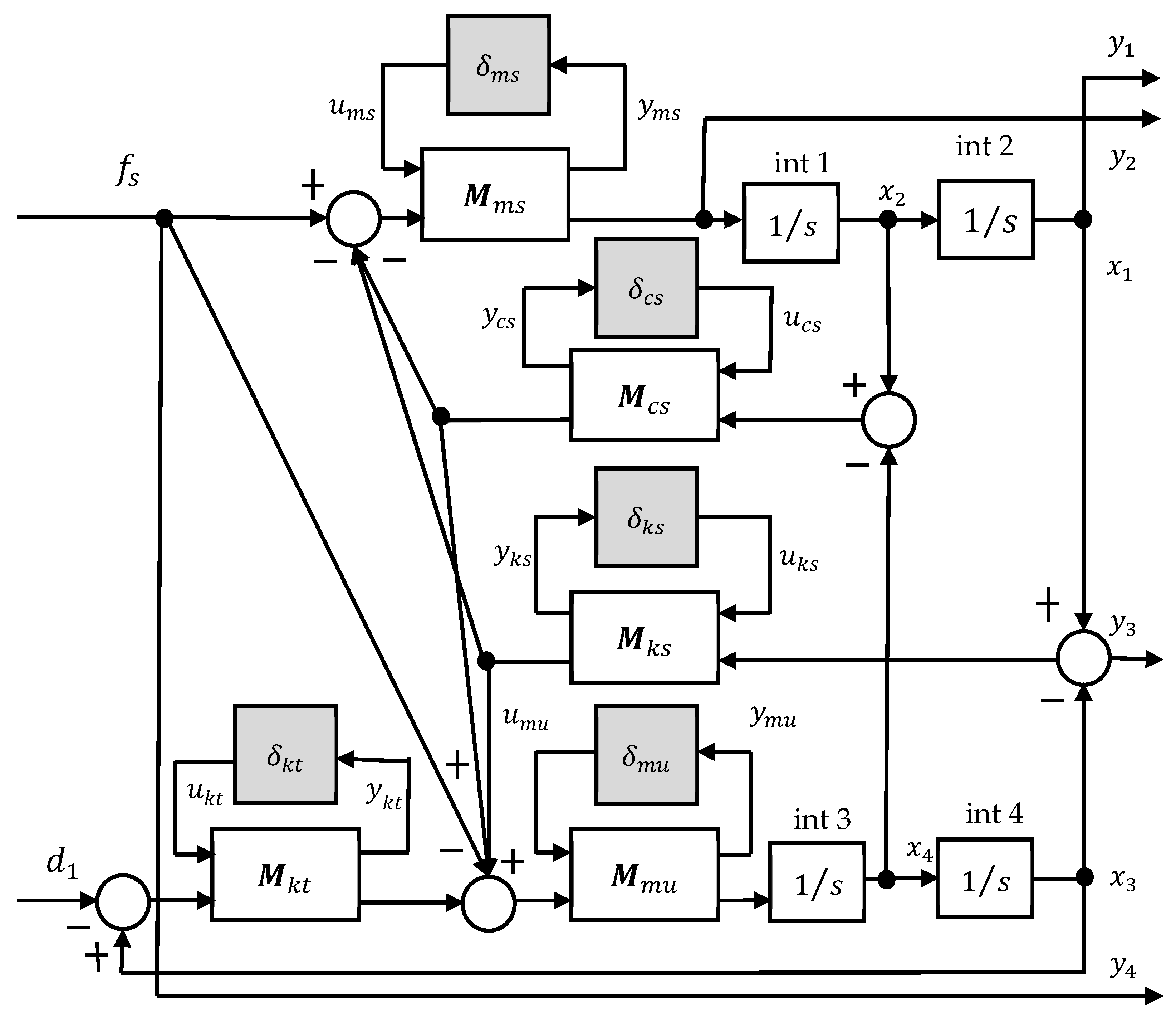
where ${\overline{c}}_s$, ${\overline{k}}_s$, ${\overline{k}}_t$, ${\overline{m}}_s$, and ${\overline{m}}_u$ are the nominal values of the system parameters $c_s$, $k_s$, $k_t$, $m_s$, and $m_u$, respectively, similarly $p_{cs}$, $p_{ks}$, $p_{kt}$, $p_{ms}$, and $p_{mu}$ the respectively possible relative variations, and ${\delta }_{ks}$, ${\delta }_{ks}$, ${\delta }_{kt}$, ${\delta }_{ms}$ and ${\delta }_{mu}$ variable coefficients, which are bounded as $-1\le {\delta }_{ij}\le 1$. The system parameters with uncertainties can be represented as upper linear fractional transformations (LFTs) [16] as $F_u\left(M_{cs},{\delta }_{cs}\right)$, $F_u\left(M_{ks},{\delta }_{ks}\right)$, $F_u\left(M_{kt},{\delta }_{kt}\right)$, $F_u\left(M_{ms},{\delta }_{ms}\right)$, and $F_u\left(M_{mu},{\delta }_{mu}\right)$ with:

$$M_{cs}=\left[\begin{array}{cc}0& {\overline{c}}_s\\ p_{cs}& {\overline{c}}_s\end{array}\right],$$

(3a)

$$M_{ks}=\left[\begin{array}{cc}0& {\overline{k}}_s\\ p_{ks}& {\overline{k}}_s\end{array}\right],$$

(3b)

$$M_{kt}=\left[\begin{array}{cc}0& {\overline{k}}_t\\ p_{kt}& {\overline{k}}_t\end{array}\right],$$

(3c)

$$M_{ms}=\left[\begin{array}{cc}-p_{ms}& \raisebox{1ex}{$1$}\!\left/ \!\raisebox{-1ex}{${\overline{m}}_s$}\right.\\ -p_{ms}& \raisebox{1ex}{$1$}\!\left/ \!\raisebox{-1ex}{${\overline{m}}_s$}\right.\end{array}\right],$$

(3d)

$$M_{ms}=\left[\begin{array}{cc}-p_{mu}& \raisebox{1ex}{$1$}\!\left/ \!\raisebox{-1ex}{${\overline{m}}_u$}\right.\\ -p_{mu}& \raisebox{1ex}{$1$}\!\left/ \!\raisebox{-1ex}{${\overline{m}}_u$}\right.\end{array}\right].$$

(3e)

Figure 2 illustrates the block diagram to represent the 2-DOF vehicle model with system parameters featured with uncertainties defined by Equations (2a–e) and (3a–e). With the above-defined system parameters with uncertainties, Equation (1a,b), which represents the dynamics of the 2-DOF vehicle model shown in Figure 1, can be rewritten as:

$$\left[\begin{array}{c}\dot{\mathit{x}}\\ {\mathit{y}}_{un}\\ \mathit{y}\end{array}\right]=\left[\begin{array}{ccc}\mathit{A}& {\mathit{B}}_1& {\mathit{B}}_2\\ {\mathit{C}}_1& {\mathit{D}}_{11}& {\mathit{D}}_{12}\\ {\mathit{C}}_2& {\mathit{D}}_{21}& {\mathit{D}}_{22}\end{array}\right]\left[\begin{array}{c}\mathit{x}\\ {\mathit{P}}_{ert}\\ \mathit{u}\end{array}\right],$$

(4a)

$${\mathit{P}}_{ert}=\Delta {\mathit{y}}_{un},$$

(4b)

where matrix $\Delta$, vector ${\mathit{y}}_{un}$, and ${\mathit{P}}_{ert}$ are defined as follows:

$$\Delta =diag\left[\begin{array}{ccc}{\delta }_{cs}& {\delta }_{ks}& \begin{array}{cc}{\delta }_{kt}& \begin{array}{cc}{\delta }_{ms}& {\delta }_{mu}\end{array}\end{array}\end{array}\right],$$

(5a)

$${\mathit{y}}_{un}={\left[\begin{array}{ccc}{y}_{cs}& y_{ks}& \begin{array}{ccc}{y}_{kt}& y_{ms}& y_{mu}\end{array}\end{array}\right]}^T,$$

(5b)

$${\mathit{P}}_{ert}={\left[\begin{array}{ccc}{u}_{cs}& u_{ks}& \begin{array}{ccc}{u}_{kt}& u_{ms}& u_{mu}\end{array}\end{array}\right]}^T,$$

(5c)

and matrices ${\mathit{B}}_1$, ${\mathit{C}}_1$, ${\mathit{D}}_{11}$, ${\mathit{D}}_{12}$, as well as ${\mathit{D}}_{21}$ are provided in Appendix A.

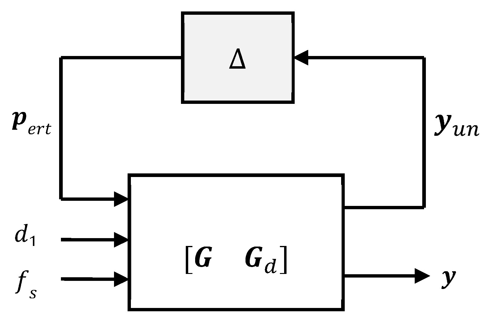
Extracting parametric uncertainties, Equation (3a–e) can be described in an LFT form as illustrated in Figure 3, in which $\mathit{G}$ and ${\mathit{G}}_d$ denote the transfer function of control input and road disturbance, respectively, and $\Delta$ is the diagonal parametric uncertainty matrix with singular values equal or less than unity.

3. Controller Design

This section first introduces the controller design problem, then formulates the design problem, and ends with describing the $H_{\infty }$ LSC controller.

3.1. Controller Design Problem

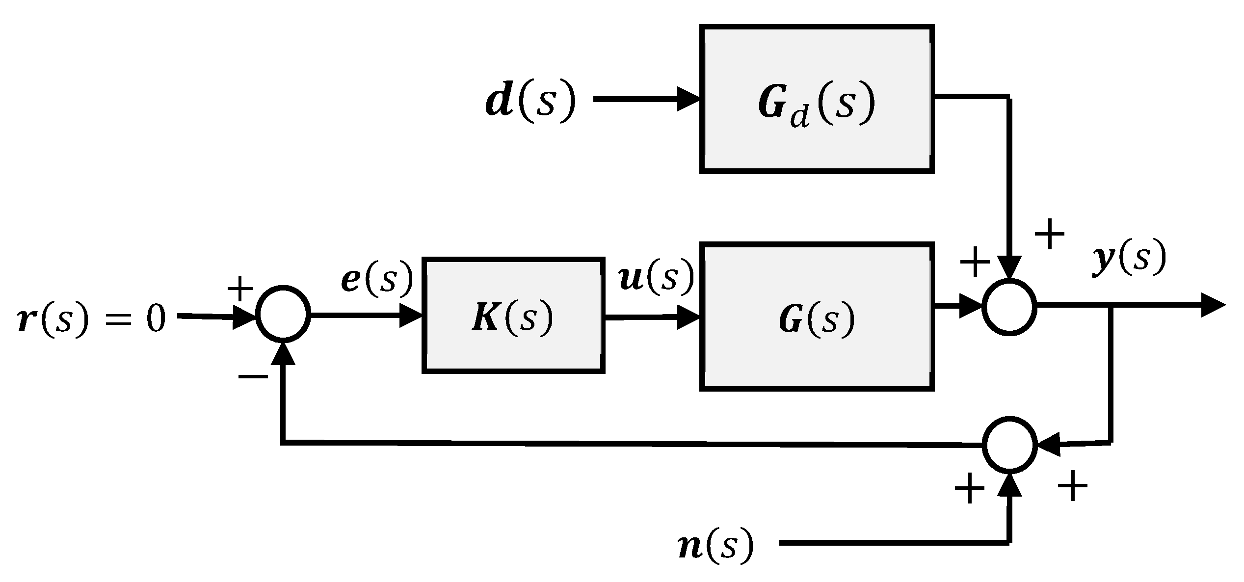
To design the controller for active suspension using the $H_{\infty }$ control technique, the vehicle dynamic system is represented as a control structure in the frequency domain as shown in Figure 4. As shown in the figure, $\mathit{r}\left(s\right)$ represents the reference input, $\mathit{e}\left(s\right)$ the tracking error, $\mathit{u}\left(s\right)$ the control input, $\mathit{d}\left(s\right)$ the external (e.g., road) disturbance, $\mathit{y}\left(s\right)$ the output, $\mathit{n}\left(s\right)$ the noise of measurement, and $\mathit{K}\left(s\right)$ the $H_{\infty }$ LSC controller to be devised. We define the output $\mathit{y}\left(s\right)$, tracking error $\mathit{e}\left(s\right)$, and control input $\mathit{u}\left(s\right)$ as:

$$\mathit{y}\left(s\right)=\mathit{T}\left(s\right)\mathit{r}\left(s\right)+\mathit{S}\left(s\right){\mathit{G}}_d\left(s\right)\mathit{d}\left(s\right)-\mathit{T}\left(s\right)\mathit{n}\left(s\right),$$

(6a)

$$\mathit{e}\left(s\right)=\mathit{S}\left(s\right)\mathit{r}\left(s\right)-\mathit{S}\left(s\right){\mathit{G}}_d\left(s\right)\mathit{d}\left(s\right)-\mathit{S}\left(s\right)\mathit{n}\left(s\right),$$

(6b)

$$\mathit{u}\left(s\right)=\mathit{S}\left(s\right)\mathit{K}\left(s\right)\mathit{r}\left(s\right)-\mathit{S}\left(s\right)\mathit{K}\left(s\right){\mathit{G}}_d\left(s\right)\mathit{d}\left(s\right)-\mathit{S}\left(s\right)\mathit{K}\left(s\right)\mathit{n}\left(s\right),$$

(6c)

where $\mathit{L}\left(s\right)=\mathit{G}\left(s\right)\mathit{K}\left(s\right)$ denotes the loop transfer function, $\mathit{S}\left(s\right)={\left[\mathit{I}+\mathit{G}\left(s\right)\mathit{K}\left(s\right)\right]}^{-1}$ the sensitivity function, $\mathit{T}\left(s\right)={\left[\mathit{I}+\mathit{G}\left(s\right)\mathit{K}\left(s\right)\right]}^{-1}\mathit{G}\left(s\right)\mathit{K}\left(s\right)$ the complementary sensitivity function [27], which is subjected to the conservation law specified as [28],

$$\mathit{I}=\mathit{S}\left(s\right)+\mathit{T}\left(s\right).\mathit{ }$$

(7)

With the consideration of additive modeling errors and removing the road disturbance for simplicity, we illustrate the control system in the block diagram shown in Figure 5, in which $\Delta \left(s\right)$ denotes the modeling uncertainty. The transfer function between the uncertain input and output can be expressed as:

$$\mathit{w}\left(s\right)=-\mathit{T}\left(s\right)\mathit{\nu }\left(s\right).\mathit{ }$$

(8)

In a controller design, the following performance criteria are usually considered [8,9,14]: command following (CF), disturbance rejection (DR), measurement-noise attenuation (MNA), control sensitivity minimization (CSM), and robustness to modeling errors (RME). To achieve the objectives, the design principle is followed: (1) effectively manipulating the controller $\mathit{K}\left(s\right)$ to minimize the sensitivity function $\mathit{S}\left(s\right)$ for improving CF and DR at low frequency; and (2) appropriately tuning the complementary function $\mathit{T}\left(s\right)$ for enhancing MNA, CSM and RME at high frequency.

3.2. Design Problem Formulation

The active suspension control design is to search for a solution in terms of the $H_{\infty }$ LSC controller, which stabilizes the vehicle system in the presence of potential perturbations, parametric uncertainties, and unmodeled dynamics. To realize the desired stability and design criteria, the controller is devised by solving two optimization problems in a frequency range of interest. The design objective is formulated as a cost function:

$$\underset{\mathit{K}\left(j\omega \right)}{\min }\left|\right|{\begin{array}{c}\mathit{S}\left(j\omega \right){\mathit{G}}_d\left(j\omega \right)\\ \mathit{T}\left(j\omega \right)\end{array}\left|\right|}_{\infty }=\underset{\mathit{K}\left(j\omega \right)}{\min }\left|\right|{\begin{array}{c}{\left[\mathit{I}+\mathit{G}\left(j\omega \right)\mathit{K}\left(j\omega \right)\right]}^{-1}{\mathit{G}}_d\left(j\omega \right)\\ {\left[\mathit{I}+\mathit{G}\left(j\omega \right)\mathit{K}\left(j\omega \right)\right]}^{-1}{\mathit{G}}_d\left(j\omega \right)\mathit{K}\left(j\omega \right)\end{array}\left|\right|}_{\infty }.$$

(9)

The first optimization problem is to ensure desired CF and DR, while the second one intends to guarantee the required MNA, CSM, and RME. Formulation (9) is the so-called S over T mixed sensitivity optimization [16]. These optimization problems cannot be solved without considering a frequency range preference due to the conservation law expressed in Equation (7), that is, minimizing one while maximizing the other. The cure to this dilemma is the frequency shaping technique, which introduces weighting functions ${\mathit{W}}_S\left(j\omega \right)$ and ${\mathit{W}}_T\left(j\omega \right)$ as:

$$\underset{\mathit{K}\left(j\omega \right)}{\min }\left|\right|{\begin{array}{c}{\mathit{W}}_S\left(j\omega \right)\mathit{S}\left(j\omega \right){\mathit{G}}_d\left(j\omega \right)\\ {\mathit{W}}_T\left(j\omega \right)\mathit{T}\left(j\omega \right)\end{array}\left|\right|}_{\infty }=\underset{\mathit{K}\left(j\omega \right)}{\min }\left|\right|{\begin{array}{c}{\mathit{W}}_S\left(j\omega \right){\left[\mathit{I}+\mathit{G}\left(j\omega \right)\mathit{K}\left(j\omega \right)\right]}^{-1}{\mathit{G}}_d\left(j\omega \right)\\ {\mathit{W}}_T\left(j\omega \right){\left[\mathit{I}+\mathit{G}\left(j\omega \right)\mathit{K}\left(j\omega \right)\right]}^{-1}{\mathit{G}}_d\left(j\omega \right)\mathit{K}\left(j\omega \right)\end{array}\left|\right|}_{\infty }.$$

(10)

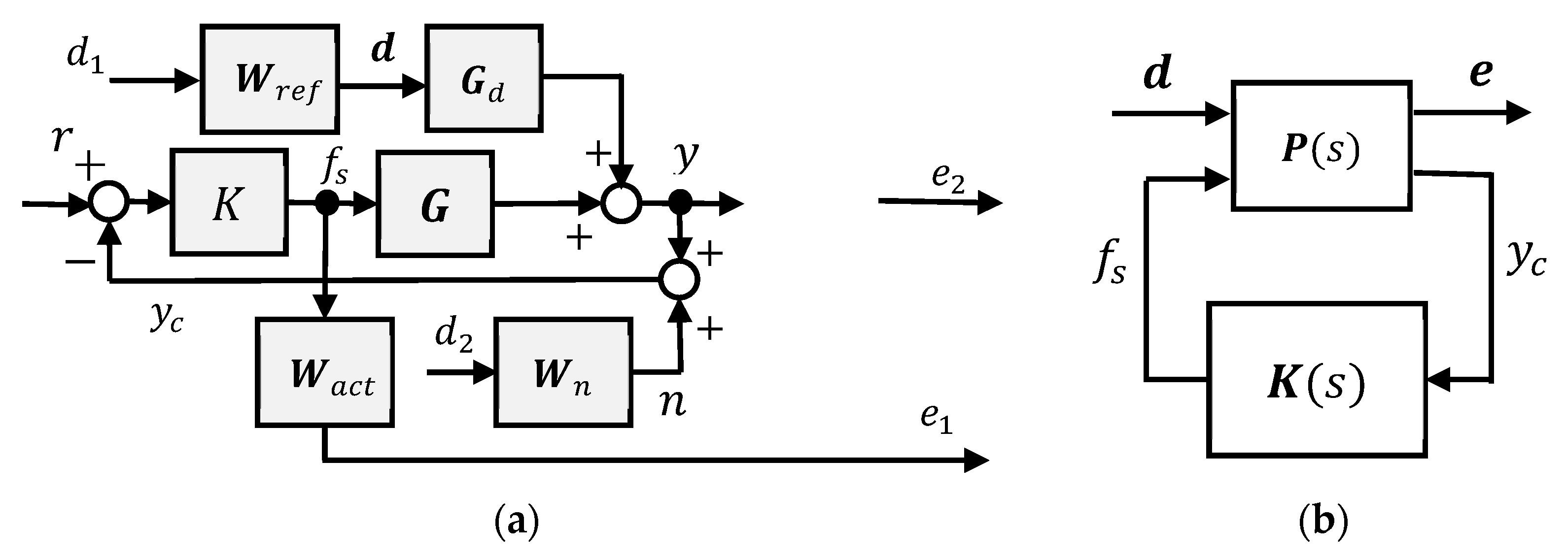
The weighting functions, ${\mathit{W}}_S\left(j\omega \right)$ and ${\mathit{W}}_T\left(j\omega \right)$, are introduced so that they have similar shapes of frequency response features, and can thus be minimized simultaneously. These weighting functions are chosen from the proper, minimum phase transfer functions of the low- or high-pass filters, depending on the application purpose [29]. A high-pass weighting function ${\mathit{W}}_T\left(j\omega \right)$ is used to shrink the space of $\mathit{T}\left(j\omega \right)$ at high frequency, while a low-pass weighting function ${\mathit{W}}_S\left(j\omega \right)$ is utilized to squeeze the space of $\mathit{S}\left(j\omega \right)$ at low frequency. The resulting active suspension systems and the respective LFT form are illustrated in Figure 6a,b, accordingly. In Figure 6b, $\mathit{P}\left(s\right)$ represents the vehicle suspension model, which consists of $\mathit{G}\left(s\right)$, ${\mathit{G}}_d\left(s\right)$, parametric uncertainties, as well as the respective weighting functions, exogenous inputs, and exogenous outputs. The active suspension system transfer function matrix, its state-space representation, input, and output interrelationship are expressed as:

$$\mathit{P}\left(s\right)=\left[\begin{array}{ccc}\mathbf{0}& \mathbf{0}& {\mathit{w}}_{act}\left(s\right)\\ {\mathit{W}}_p\left(s\right){\mathit{G}}_d\left(s\right){\mathit{W}}_{ref}\left(s\right)& \mathbf{0}& {\mathit{W}}_p\left(s\right)\mathit{G}\left(s\right)\\ {\mathit{G}}_d\left(s\right){\mathit{W}}_{ref}\left(s\right)& {\mathit{W}}_n\left(s\right)& \mathit{G}\left(s\right)\end{array}\right]\stackrel{\mathrm{def}}{=}\left[\begin{array}{ccc}{\mathit{A}}_w& {\mathit{B}}_{1w}& {\mathit{B}}_{2w}\\ {\mathit{C}}_{1w}& {\mathit{D}}_{11w}& {\mathit{D}}_{12w}\\ {\mathit{C}}_{2w}& {\mathit{D}}_{21w}& {\mathit{D}}_{22w}\end{array}\right],$$

(11a)

$$\mathit{e}=F_l\left[\mathit{P}\left(s\right), \mathit{K}\left(s\right)\right]\mathit{d},$$

(11b)

where ${\mathit{W}}_p\left(s\right)$, ${\mathit{W}}_{ref}\left(s\right)$, ${\mathit{W}}_n\left(s\right)$ and ${\mathit{w}}_{act}\left(s\right)$ are the weighting matrix of the system output vector ${\left[\begin{array}{ccc}{x}_1& {\ddot{x}}_1& x_1-x_3\end{array}\right]}^T$, weighting function of road disturbance $d_1$, weighting function of measurement noise $d_2$, and weighting function of suspension actuator force $f_s$, respectively, ${\mathit{A}}_w$, ${\mathit{B}}_{1w}$, ${\mathit{B}}_{2w}$, ${\mathit{C}}_{1w}$, ${\mathit{C}}_{2w}$, ${\mathit{D}}_{11w}$, ${\mathit{D}}_{12w}$, ${\mathit{D}}_{21w}$, and ${\mathit{D}}_{22w}$ denote the weighting matrices of the matrices $\mathit{A}$, ${\mathit{B}}_1$, ${\mathit{B}}_2$, ${\mathit{C}}_1$, ${\mathit{C}}_2$, ${\mathit{D}}_{11}$, ${\mathit{D}}_{12}$, ${\mathit{D}}_{21}$, and ${\mathit{D}}_{22}$ in Equation (4a), $\mathit{d}={\left[\begin{array}{cc}{d}_1& d_2\end{array}\right]}^T$, and $\mathit{e}={\left[\begin{array}{cc}\begin{array}{cc}{e}_1& e_2\end{array}& \begin{array}{cc}{e}_3& e_4\end{array}\end{array}\right]}^T$, denoting the tracking errors of the four state variables, and $F_l\left[\mathit{P}\left(s\right), \mathit{K}\left(s\right)\right]$ is the lower linear fractional transformation of $\mathit{P}$ and $\mathit{K}$ [16].

3.3. $H_{\infty }$ Loop-Shaping Controller

An $H_{\infty }$ loop-shaping controller is devised for the weighted active suspension system by solving an optimization problem. For the $H_{\infty }$ LSC optimization designs, the small-gain theorem provides a sufficient and necessary condition [16], which can be expressed as:

$$\left|\right|F_l\left[\mathit{P}\left(s\right), \mathit{K}\left(s\right)\right]\mathit{d}{||}_{\infty }<1,$$

(12)

which implies:

• Nominal stability and performance. The $H_{\infty }$ LSC controller ensures that the closed-loop system is internally stable, and the desired closed-loop responses are achieved for the nominal vehicle suspension model.
• Robust stability and performance. The $H_{\infty }$ LSC controller guarantees that the closed-loop system is internally stable, and the desired closed-loop responses are obtained for all possible vehicle suspension models with parametric uncertainties.

While satisfying the condition specified by (12), there exist three algorithms for solving the optimization problem defined in (10). The solutions are three designs: (1) an $H_{\infty }$ suboptimal controller, (2) an $H_{\infty }$ LSC controller, and (3) an $\mu$ analysis and synthesis controller [16]. In this study, an $H_{\infty }$ LSC controller is devised.

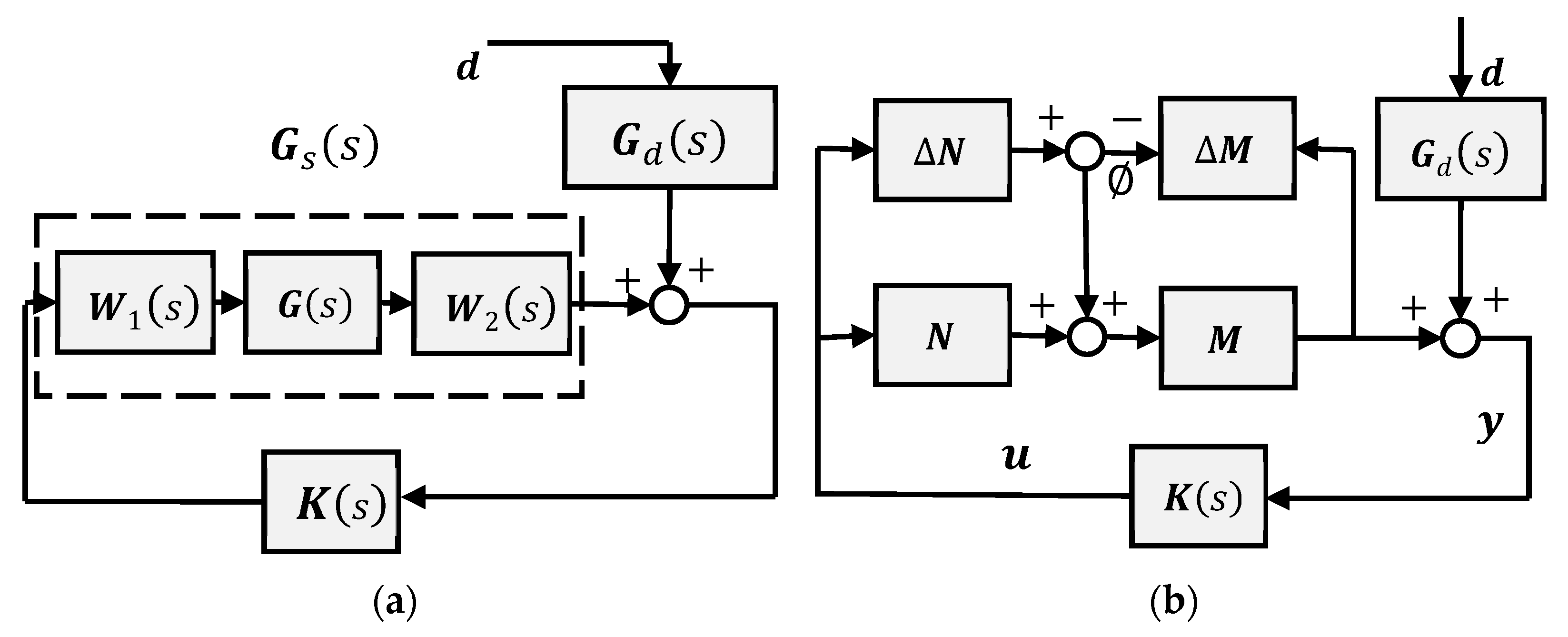
The design of the $H_{\infty }$ LSC controller follows a two-step procedure. First, the vehicle suspension system is pre- and post-compensated to shape the open-loop frequency response [29]. Second, the shaped vehicle suspension system is stabilized with a controller as illustrated in Figure 7a. For simplicity, several weighting functions are removed.

Given the state-space equation defined in Equation (1a,b) for representing the vehicle system, transfer function matrix $\mathit{G}\left(s\right)$ can be derived using Laplace transform with the assumption of zero initial condition of the state variables. Similarly, for the resulting pre- and post-weighted transfer function matrix ${\mathit{G}}_s\left(s\right),$ the open-loop transfer function and the respective state-space model of the shaped vehicle suspension model can be cast as:

$${\mathit{G}}_s\left(s\right)={\mathit{W}}_1\left(s\right)\mathit{G}\left(s\right){\mathit{W}}_2\left(s\right)={\mathit{D}}_s+{\mathit{C}}_s{\left(s\mathit{I}-{\mathit{A}}_s\right)}^{-1}{\mathit{B}}_s\stackrel{\mathrm{def}}{=}\left[\begin{array}{cc}{\mathit{A}}_s& {\mathit{B}}_s\\ {\mathit{C}}_s& {\mathit{D}}_s\end{array}\right],$$

(13)

where matrices ${\mathit{A}}_s$, ${\mathit{B}}_s$, ${\mathit{C}}_s$, and ${\mathit{D}}_s$ are the counterparts of $\mathit{A}$, ${\mathit{B}}_2$, ${\mathit{C}}_2$, and ${\mathit{D}}_{22}$ in Equation (1a,b), ${\mathit{W}}_1\left(s\right)$ and ${\mathit{W}}_2\left(s\right)$ denote the weighting functions for pre- and post-compensating the suspension system to shape the open-loop response, respectively.

To constitute a left coprime factorization of the shaped vehicle suspension model [16], it is assumed that the weighted transfer function matrix ${\mathit{G}}_s\left(s\right)$ can be expressed as:

$${\mathit{G}}_s\left(s\right)={\mathit{M}}^{-1}\left(s\right)\mathit{N}\left(s\right).\mathit{ }$$

(14)

For ${\mathit{G}}_s\left(s\right)$, the normalized left coprime factorization can be derived by solving the filter algebraic Riccati equation:

$$\left({\mathit{A}}_s-{\mathit{B}}_s{\mathit{D}}_s^T{\mathit{R}}^{-1}{\mathit{C}}_s\right){\mathit{Z}}_s+{\mathit{Z}}_s{\left({\mathit{A}}_s-{\mathit{B}}_s{\mathit{D}}_s^T{\mathit{R}}^{-1}{\mathit{C}}_s\right)}^T-{\mathit{Z}}_s{\mathit{C}}_s^T{\mathit{R}}^{-1}{\mathit{C}}_s{\mathit{Z}}_s+{\mathit{B}}_s\left(\mathit{I}-{\mathit{D}}_s^T{\mathit{R}}^{-1}{\mathit{D}}_s\right){\mathit{B}}_s^T=0,$$

(15)

where the solution, i.e., the normalized left coprime factorization is:

$$\left[\begin{array}{cc}\mathit{N}\left(s\right)& \mathit{M}\left(s\right)\end{array}\right]\stackrel{\mathrm{def}}{=}\left[\begin{array}{ccc}{\mathit{A}}_s+\mathit{H}{\mathit{C}}_s& {\mathit{B}}_s+\mathit{H}{\mathit{D}}_s& \mathit{H}\\ {\mathit{R}}^{-1/2}{\mathit{C}}_s& {\mathit{R}}^{-1/2}{\mathit{D}}_s& {\mathit{R}}^{-1/2}\end{array}\right],$$

(16)

with $H=-\left(Z_s{\mathit{C}}_s^T+{\mathit{B}}_s{\mathit{D}}_s^T\right){\mathit{R}}^{-1}$, $\mathit{R}\stackrel{\mathrm{def}}{=}\mathit{I}+{\mathit{D}}_s{\mathit{D}}_s^T$, and ${\mathit{Z}}_s\ge \mathbf{0}$.

The LSC controller is devised as a robust stabilizer with the left coprime factorized uncertainties and the road disturbance as shown in Figure 7b. Note that considering the introduced perturbations, i.e., $\Delta \mathit{M}$ and $\Delta \mathit{N}$, shown in Figure 7b, the perturbed vehicle system transfer function can be described by:

$${\mathit{G}}_{s\Delta }\left(s\right)={\left(\mathit{M}\left(s\right)+\Delta \mathit{M}\left(s\right)\right)}^{-1}\left(\mathit{N}\left(s\right)+\Delta \mathit{N}\left(s\right)\right),\mathit{ }$$

(17)

where $\Delta \mathit{M}$ and $\Delta \mathit{N}$ are unknown but stable transfer functions, which denote the uncertainty in the nominal vehicle system model. The design objective of robust stabilization is to stabilize not only the nominal vehicle model ${\mathit{G}}_s\left(s\right)$, but also the perturbed model ${\mathit{G}}_{s\Delta }\left(s\right)$.

To maximize the robust stability of the closed-loop vehicle system shown in Figure 7b, we need to minimize:

$$\gamma \stackrel{\mathrm{def}}{=}{\left|\right|\left[\begin{array}{cc}\mathit{I}& \mathit{K}\end{array}\right]}^T{\left(\mathit{I}-{\mathit{G}}_s\mathit{K}\right)}^{-1}{\mathit{M}}^{-1}\left|\right|{}_{\infty }\mathit{ }$$

(18)

The achievable minimum value of $\gamma$ for all stabilizing controllers $\mathit{K}$ is given by:

$${\gamma }_{min}={\left\{1-{\lambda }_{max}\left[{\mathit{Z}}_s{\mathit{X}}_s{\left(\mathit{I}+{\mathit{Z}}_s{\mathit{X}}_s\right)}^{-1}\right]\right\}}^{-1/2},$$

(19)

where ${\lambda }_{max}(\dot{})$ represents the maximum eigenvalue, and ${\mathit{X}}_s$ is the solution of the algebraic Riccati equation,

$${\left({\mathit{A}}_s-{\mathit{B}}_s{\mathit{S}}^{-1}{\mathit{D}}_s^T{\mathit{C}}_s\right)}^T{\mathit{X}}_s+{\mathit{X}}_s\left({\mathit{A}}_s-{\mathit{B}}_s{\mathit{S}}^{-1}{\mathit{D}}_s^T{\mathit{C}}_s\right)-{\mathit{X}}_s{\mathit{B}}_s{\mathit{S}}^{-1}{\mathit{B}}_s^T{\mathit{X}}_s+{\mathit{C}}_s^T\left(\mathit{I}-{\mathit{D}}_s{\mathit{S}}^{-1}{\mathit{D}}_s^T\right){\mathit{C}}_s=\mathbf{0},$$

(20)

where $\mathit{S}=\mathit{I}+{\mathit{D}}_s^T{\mathit{D}}_s$. Thus, with $\gamma >{\gamma }_{min}$, an LSC controller $\mathit{K}$ can be found from the state-space and described by:

$${\mathit{K}}_s\stackrel{\mathrm{def}}{=}\left[\begin{array}{cc}{\mathit{A}}_s+{\mathit{B}}_s\mathit{F}+{\gamma }^2{\left({\mathit{L}}^T\right)}^{-1}{\mathit{Z}}_s{\mathit{C}}_s^T\left({\mathit{C}}_s+{\mathit{D}}_s\mathit{F}\right)& {\gamma }^2{\left({\mathit{L}}^T\right)}^{-1}{\mathit{Z}}_s{\mathit{C}}_s^T\\ {\mathit{B}}_s^T{\mathit{X}}_s& -{\mathit{D}}_s^T\end{array}\right],$$

(21)

where $\mathit{F}=-{\mathit{S}}^{-1}\left({\mathit{D}}_s^T{\mathit{C}}_s+{\mathit{B}}_s^T{\mathit{X}}_s\right)$ and $\mathit{L}=\left(1-{\gamma }^2\right)\mathit{I}+{\mathit{X}}_s{\mathit{Z}}_s$.

4. Proposed Design Synthesis Method

Figure 8 shows the proposed design synthesis method for robust controllers of active vehicle suspensions. This is a two-layer design optimization approach. In the design optimization of the $H_{\infty }$ loop-shaping controller for AVSs, all the parameters for the relevant weighting functions of the controller are treated as design variables. Initially, n sets of the design variables are randomly selected in the design space by a genetic algorithm (GA) at the top layer [30]. Considering the expensive computational loads due to the application of the GA, we use the parallel computing technique available in Matlab [31]. The scheduler parallelly sends each of the n design variable sets to the respective Worker of the parallel computing system. At the bottom layer, with a given design variable set, such as set i, the respective Worker i ‘operates’ the virtual vehicle with the $H_{\infty }$ LSC-based AVS under a specified testing maneuver. After the virtual testing, the required performance measures denoted by ${\overline{M}}_{i,j} \left(j=1,2,\dots , N\right)$, which are acquired from the respective numerical simulation response. After the virtual test for all the Workers from $\mathbf{1} \mathrm{to} n$, we can achieve a performance measure matrix ${\overline{M}}_{i,j}$ with the size of $n\times N$. With the performance measure matrix, the defined constraints and the objective function are evaluated.

Similar to the cost function defined in [8], in this research, we specify the objective function at the top layer as:

$$J=\frac{{\sigma }_1{\phi }_1}{{\phi }_1^p}+\frac{{\sigma }_2{\phi }_2}{{\phi }_2^p}+\frac{{\sigma }_3{\phi }_3}{{\phi }_3^p}+\frac{{\sigma }_4{\phi }_4}{{\phi }_4^p},$$

(22)

where ${\sigma }_i$, $i=1,2,3,4,$ are weighting factors, ${\phi }_1$, ${\phi }_2$, ${\phi }_3$, and ${\phi }_4$ are the root mean square (RMS) values of the vertical acceleration of sprung mass, vertical acceleration of unsprung mass, suspension dynamic deflection, and wheel deflection achieved by the $H_{\infty }$ LSC-based AVS, while ${\phi }_1^p$, ${\phi }_2^p$, ${\phi }_3^p$, and ${\phi }_4^p$ represent the RMS values of the passive suspension relative to ${\phi }_1$, ${\phi }_2$, ${\phi }_3$, and ${\phi }_4$, respectively. With the objective function defined by (22), the number ($N$) of performance measures acquired for each virtual testing during the process shown in Figure 8 is 4, and we have the performance measure matrix ${\overline{M}}_{i,j}$ with the size of $n\times 4$ after the virtual test for all the Workers from $1 \mathrm{to} n$. Note that the number ($n$) of Workers of the design optimization is dependent on the slave notes of the master-slave computer cluster used for the design optimization [32,33]. In (22), the objective function is formulated in the form of the so-called scalarization [34,35], which converts a multi-objective optimization problem into a single objective one. This will significantly facilitate design optimization. The use of normalization aims at ensuring the same order of digital value of each performance measure involved in the objective function.

After the objective function evaluations, the performance index vector, i.e., ${\left[J_1, J_2, \dots , J_n\right]}^T$, is achieved for the n sets of design variables. At this point, if the convergence criteria, e.g., a predefined total generation number, an acceptable error between the best objective function values of the last two generations, etc., are satisfied, the optimization process terminates; otherwise, this performance index vector is feedbacked to the GA at the top layer. Based on the returned performance index values corresponding to the given sets of design variables, the GA creates the next generation of design variable sets using genetic operators, such as selection, crossover, and mutation. This process repeats until the optimal variable set, i.e., the best weighting function parameter set for the $H_{\infty }$ LSC controller is identified.

5. Results and Discussion

To perform the design optimization of the vehicle suspension system with the $H_{\infty }$ loop-shaping controller, the vehicle model parameters take the nominal values listed in

Table 1. The nominal parameter values of the passive vehicle suspension system [36].

${\mathit{m}}_{\mathit{s}} \left(\mathbf{kg}\right)$	${\mathit{m}}_{\mathit{u}} \left(\mathbf{kg}\right)$	${\mathit{k}}_{\mathit{s}} (\mathbf{N}/\mathbf{m})$	${\mathit{c}}_{\mathit{s}} (\mathbf{N}/\mathbf{m}/\mathbf{s})$	${\mathit{k}}_{\mathit{t}} (\mathbf{N}/\mathbf{m})$
299.0	59.0	16,182.0	1000	190,000

. To assess the performance of the AVS designs, the road disturbance is defined by:

$$d_1\left(t\right)=\{\begin{array}{cc}0.025\left[1-cos\left(8\pi t\right)\right],& 0\le t\le 0.25\\ 0& otherwise\end{array},$$

(23)

Table 2. Weighting functions devised with conventional frequency shaping technique.

${\mathit{W}}_{\mathit{r}\mathit{e}\mathit{f}} \left(\mathit{s}\right)$	${\mathit{W}}_{\mathit{n}} \left(\mathit{s}\right)$	${\mathit{W}}_{\mathit{a}\mathit{c}\mathit{t}} \left(\mathit{s}\right)$	${\mathit{W}}_{{\mathit{x}}_{\mathbf{1}}} \left(\mathit{s}\right)$
$\frac{0.0633}{0.0798s+1}$	0.0157	$\frac{8.658s+77.88}{s+140.7}$	$\frac{16.35}{s^2+8.678s+17.91}$
${\mathit{W}}_{{\ddot{\mathit{x}}}_{\mathbf{1}}} \left(\mathit{s}\right)$	${\mathit{W}}_{{\mathit{x}}_{\mathbf{1}}-{\mathit{x}}_{\mathbf{2}}} \left(\mathit{s}\right)$	${\mathit{W}}_{\mathbf{1}} \left(\mathit{s}\right)$	${\mathit{W}}_{\mathbf{2}} \left(\mathit{s}\right)$
$\frac{2.389}{0.4554s+1}$	$\frac{10.28}{0.0786s+1}$	$\frac{2.474e7s+4.768e7}{s+3859}$	1

lists the weighting functions and compensators, which are designed with the conventional frequency shaping technique [27,28]. These weighting functions are applied to road disturbance $d_1$, measurement noise $d_2$, control input $f_s$, as well as outputs $x_1$, ${\ddot{x}}_1$, and $x_1-x_2$ to reshape the closed- and open-loop frequency characteristics while designing the $H_{\infty }$ loop-shaping controllers as shown in Figure 6a and Figure 7a, respectively.

Table 3. Weighting functions devised by using the proposed design synthesis method.

${\mathit{W}}_{\mathit{r}\mathit{e}\mathit{f}} \left(\mathit{s}\right)$	${\mathit{W}}_{\mathit{n}} \left(\mathit{s}\right)$	${\mathit{W}}_{\mathit{a}\mathit{c}\mathit{t}} \left(\mathit{s}\right)$	${\mathit{W}}_{{\mathit{x}}_{\mathbf{1}}} \left(\mathit{s}\right)$
$\frac{0.1252}{0.5512s+1}$	0.0196	$\frac{1.197s+2.138}{s+58.47}$	$\frac{4.304}{s^2+6.357s+9.718}$
${\mathit{W}}_{{\ddot{\mathit{x}}}_{\mathbf{1}}} \left(\mathit{s}\right)$	${\mathit{W}}_{{\mathit{x}}_{\mathbf{1}}-{\mathit{x}}_{\mathbf{2}}} \left(\mathit{s}\right)$	${\mathit{W}}_{\mathbf{1}} \left(\mathit{s}\right)$	${\mathit{W}}_{\mathbf{2}} \left(\mathit{s}\right)$
$\frac{1.328}{0.7701s+1}$	$\frac{1.474}{0.7612s+1}$	$\frac{1.6e7s+3.7e7}{s+2791}$	1

provides the respective weighting functions derived from the design optimization using the method shown in Figure 8.

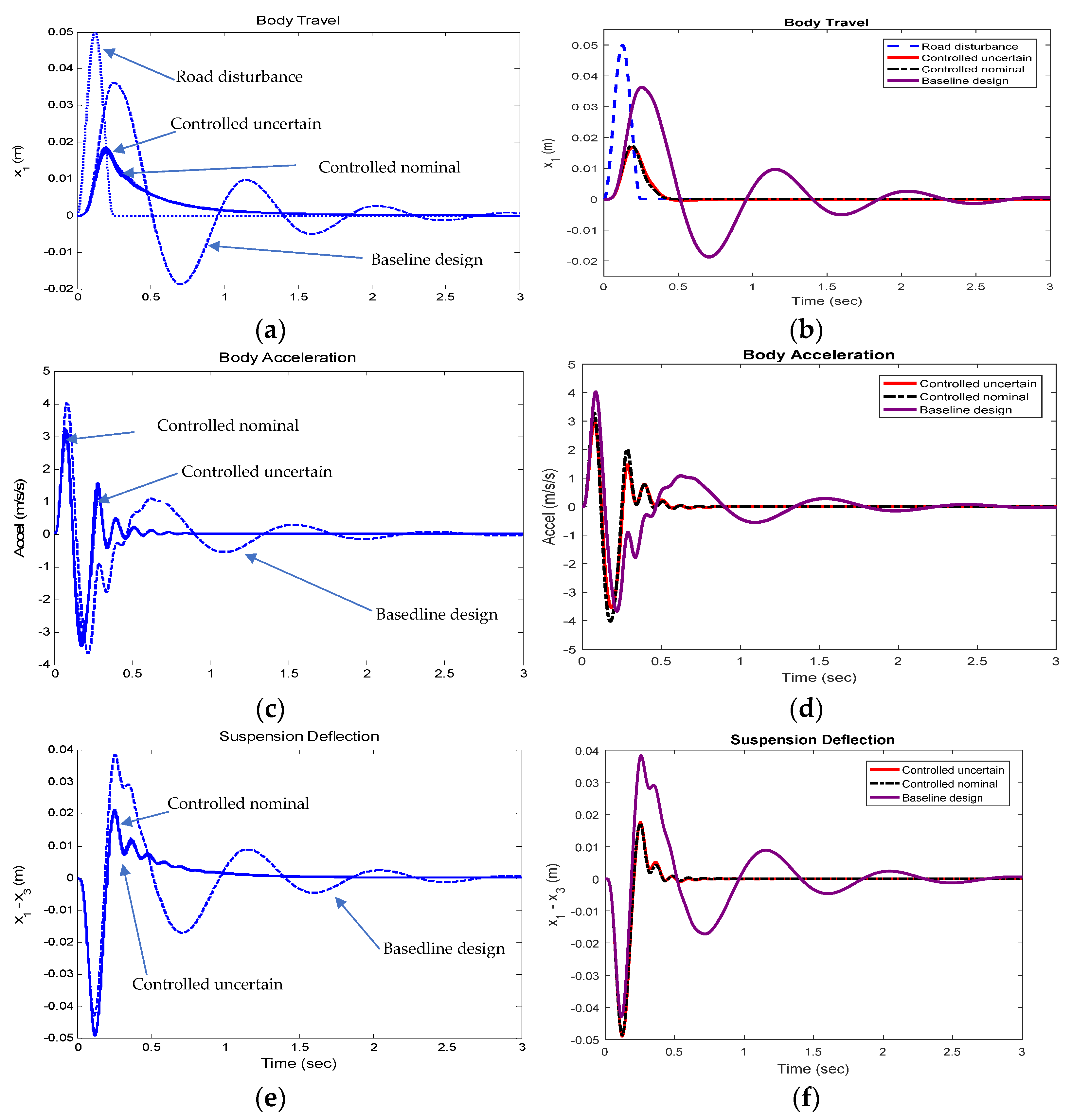
The performance of the $H_{\infty }$ LSC-based AVSs is compared against that of the baseline design. For the benchmark, three designs are considered: (1) the baseline design, i.e., the vehicle model shown in Figure 1 without the force actuator $f_s$; (2) the controlled nominal design, that is, the $H_{\infty }$ LSC-based AVS is designed with the vehicle model parameters taking the nominal values listed in Table 1 and with the application of weighting functions listed in Table 2 and Table 3 the controlled uncertain design, in which the vehicle system is modeled with uncertain parameters and the $H_{\infty }$ LSC-based AVS is optimally devised using the proposed design synthesis method. For simplicity, hereafter the three designs are denoted by Design 1, 2 and 3. For Design 3, 100 design cases are obtained with the maximum parametric uncertainty of $\pm 30\%$ for sprung mass $m_s$ and the maximum parametric uncertainty of $\pm 10\%$ for all other vehicle model parameters. The performance comparison of the three designs is shown in Figure 9.

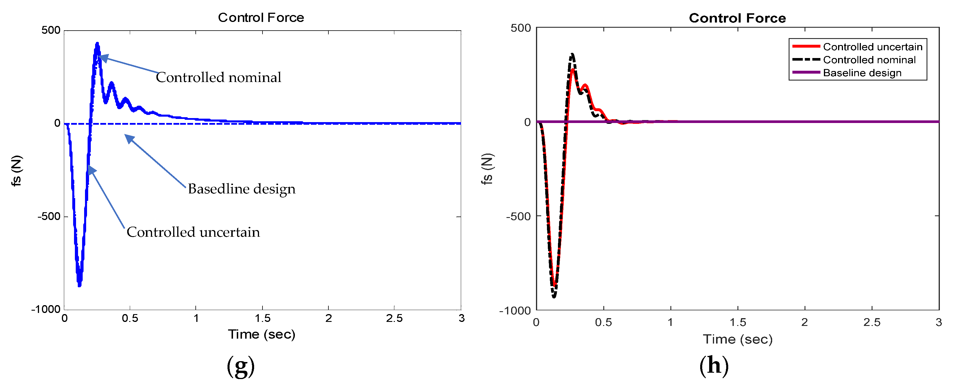
Figure 9a,c,e,g show the performance of the three designs in terms of time-history of sprung mass vertical displacement, sprung mass vertical acceleration, suspension dynamic deflection, and actuator force, respectively. Since the curves of Design 3 (with 100 design cases) overlap their counterparts of Design 2 in the aforementioned figures, and it is difficult to distinguish the curves of Design 3 from the respective curves of Design 2, we replot the curves of Designs 1 and 2 shown in Figure 9a,c,e,g in Figure 9b,d,f,h, respectively. Moreover, to facilitate the performance comparison, the curves for the average performance measures of the 100 cases of Design 3 are used to represent the performance of this design, and the respective average performance curves are also shown in Figure 9b,d,f,h.

To facilitate quantitative comparison of the performance measures among the three designs, the maximum performance measure values shown in Figure 9b,d,f,h are listed in

Table 4. Comparison of the maximum performance measure values among the three designs.

Performance Measures	Design 1	Design 2	Improvement a	Design 3 b	Improvement c
$\mathrm{maximum} \mathrm{sprung} \mathrm{mass} \mathrm{vertical} \mathrm{displacement} \left(\mathrm{m}\right)$	0.0363	0.0173	52.34%	0.0167	3.47%
$\mathrm{maximum} \mathrm{sprung} \mathrm{mass} \mathrm{vertical} \mathrm{acceleration} (\mathrm{m}⁄{\mathrm{s}}^2)$	4.0638	4.0426	0.52%	3.5532	12.11%
$\mathrm{maximum} \mathrm{suspension} \mathrm{dynamic} \mathrm{deflection} \left(\mathrm{m}\right)$	0.0433	0.0490	−13.16%	0.0495	−1.02%
$\mathrm{maximum} \mathrm{actuator} \mathrm{force} \left(\mathrm{N}\right)$		940.476		869.048	7.59%

^a Improvement: performance measure improvement of Design 2 with respect to that of Design 1. ^b Design 3: the average performance measure of the 100 design cases of Design 3. ^c Improvement: performance measure improvement of Design 3 with respect to that of Design 2.

. Compared with Design 1, Design 2 significantly reduces the maximum sprung mass travel by 52.34% and marginally decreases the maximum sprung mass vertical acceleration by 0.52% at the expense of degrading the maximum suspension dynamic deflection by 13.16% and consuming the control effort with the maximum peak actuator force of 940.476 N. Moreover, with respect to Design 1, Design 2 responds to the road disturbance faster in terms of all system outputs. A close observation of the performance difference between Designs 2 and 3 discloses that, within the given bounded model parameter variation ranges, the parametric uncertainties pose no significance on the sprung mass travel, suspension dynamic deflection, and sprung mass acceleration. To quantitatively compare the performance measures of Design 2 and 3, we assume that the latter is represented by the average design of the 100 design cases. With respect to Design 2, Design 3 improves performance by reducing the maximum sprung mass vertical displacement by 3.47%, the maximum sprung mass vertical acceleration by 12.11%, and the maximum actuator force by 7.59% at the cost of marginally increasing the maximum suspension dynamic deflection by 1.02%. Interestingly, compared with and Design 2, Design 3 improves the performance in maximum sprung mass travel, maximum sprung mass vertical acceleration, maximum control effort, and maintaining approximately the same maximum peak value of suspension deflection. This implies that the optimal design of the $H_{\infty }$ LSC controller with parameter uncertainty attenuates the level of conflicting performance measures of the AVS with a $H_{\infty }$ sub-optimal controller reported in [36]. This benefit of the $H_{\infty }$ LSC controller may be attributed to the application of the proposed design synthesis method for optimally tuning the parameters of the weighting functions to compromise the trade-offs among the conflicting performance measures of AVSs.

The above observation indicates that, for Design 3 with the given bounded model parameter variation ranges, parametric uncertainties pose minor impacts on the performance of the AVS. To further examine this issue, we conduct a parametric sensitivity analysis for this design. Each time, only one parameter is allowed to be varied and others are fixed at their nominal values. The selected parameter varies until it approaches a value, at which the controller loses its stability. This value is denoted as the threshold value of this parameter, and the variation range constrained by the threshold value is defined as the threshold uncertainty.

Table 5. The threshold uncertainties of vehicle model parameters (% of nominal values).

${\mathit{m}}_{\mathit{s}}$	${\mathit{m}}_{\mathit{u}}$	${\mathit{k}}_{\mathit{s}}$	${\mathit{c}}_{\mathit{s}}$	${\mathit{k}}_{\mathit{t}}$
100.0	25.0	41.0	21.0	39.0

lists the threshold uncertainties of all the model parameters.

6. Conclusions

This paper proposes a design synthesis method for robust controllers of active vehicle suspensions (AVSs). This method provides a framework for two-layer design optimization problems. At the top layer, the specified objective function and constraints are evaluated, and an evolutionary algorithm, i.e., a genetic algorithm, is introduced to search in the design space to find optimal design variables for the robust controller. At the bottom layer, the robust controller and the vehicle model are integrated to form a virtual vehicle with robust active suspensions. With a design variable set from the top layer, the robust controller is updated, and a numerical simulation is performed to mimic a testing maneuver and to extract performance measures from the dynamic responses of the simulation. The acquired data are feedbacked to the top layer for evaluating the objective function and constraints. The proposed method is applied to the search of optimal parameters for the weighting functions of an $H_{\infty }$ loop-shaping controller for a vehicle with AVS. To address the problem of expensive computational loads of design optimization, a parallel computing technique is recommended.

The proposed method systematically deals with parametric uncertainties and unmodelled dynamics of a vehicle model with AVS. The optimal $H_{\infty }$ loop-shaping controller designed using the method achieves robust stability and performance with specified parameter uncertainties. With the given testing condition and the specified vehicle model parameter variation ranges, compared with the $H_{\infty }$ loop-shaping controller design with the nominal model parameter values and the weighting functions determined using the conventional technique, the optimal controller design based on the proposed method improves performance by reducing the maximum sprung mass vertical displacement by 3.47%, the maximum sprung mass vertical acceleration by 12.11%, and the maximum actuator force by 7.59% at the cost of marginally increasing the maximum suspension dynamic deflection by 1.02%. With the resulting robust controller, the stability margin of the active suspension system on individual parametric uncertainties can be easily identified. The achieved parametric uncertainty thresholds may be used as a guideline for robust controller designs of active vehicle suspensions. Simulation results indicate that a compromised design solution can be achieved for the conflicting performance measures of active suspension by optimally tuning the weighting functions of the $H_{\infty }$ loop-shaping controller. The application of the proposed method can be extended to the robust controller designs for other active vehicle safety systems, e.g., active steering and anti-roll systems.

References

1. Chi, Z.; He, Y.; Naterer, G.F. Design optimization of vehicle suspensions with a quarter-vehicle model. Trans. Can. Soc. Mech. Eng. 2008, 32, 297–312. [Google Scholar] [CrossRef]
2. He, Y.; McPhee, Y. Application of optimization algorithms and multibody dynamics to ground vehicle suspension design. Int. J. Heavy Veh. Syst. 2007, 14, 158–192. [Google Scholar] [CrossRef]
3. Sohn, H.C.; Hong, K.T.; Yoo, W.S. An adaptive LQG control for semi-active suspension systems. Int. J. Veh. Des. 2004, 34, 309–325. [Google Scholar] [CrossRef]
4. Aljarbouh, A.; Fayaz, M.; Qureshi, M.S.; Boujoudar, Y. Hybrid sliding mode control of full-car semi-active suspension systems. Symmetry 2021, 13, 2442. [Google Scholar] [CrossRef]
5. He, Y.; McPhee, J. Multidisciplinary design optimization of mechatronic vehicles with active suspensions. J. Sound Vib. 2005, 283, 217–241. [Google Scholar] [CrossRef]
6. He, Y.; McPhee, J. A design methodology for mechatronic vehicles: Application of multidisciplinary optimization, multibody dynamics and genetic algorithms. Veh. Syst. Dyn. 2005, 43, 697–733. [Google Scholar] [CrossRef]
7. He, Y. Design of Rail Vehicles with Passive and Active Suspensions Using Multidisciplinary Optimization, Multibody Dynamics, and Genetic Algorithms. Ph.D. Thesis, University of Waterloo, Waterloo, ON, Canada, 2003. [Google Scholar]
8. Lee, E.; He, Y. Automated design synthesis of LQR controllers for road vehicle active suspension systems. In Proceedings of the 25th CANCAM, London, ON, Canada, 31 May–4 June 2015. [Google Scholar]
9. Miege, A.J.; Cebon, D. Optimal roll control of an articulated vehicle: Theory and model validation. Veh. Syst. Dyn. 2005, 43, 867–884. [Google Scholar] [CrossRef]
10. Fu, Z.; Dong, X. H optimal control of vehicle active suspension system in two time scales. Automatika 2021, 62, 284–292. [Google Scholar] [CrossRef]
11. Ryu, S.; Kim, Y.; Park, Y. Robust H preview control of an active suspension system with norm-bounded uncertainties. J. Automot. Technol. 2008, 9, 585–592. [Google Scholar] [CrossRef]
12. Chen, B.C.; Shiu, Y.H.; Hsieh, F.C. Sliding-mode control for semi-active suspension with actuator dynamics. Veh. Syst. Dyn. 2011, 49, 277–290. [Google Scholar] [CrossRef]
13. Koshkouei, A.J.; Burnham, K.J. Sliding mode controllers for active suspensions. In Proceedings of the 17th World Congress, the International Federation of Automatic Control, Seoul, Korea, 6–11 July 2008. [Google Scholar]
14. Yagiz, N.; Hacioglu, Y.; Taskin, Y. Fuzzy sliding-mode control of active suspensions. IEEE Trans. Ind. Electron. 2008, 55, 3883–3890. [Google Scholar] [CrossRef]
15. Aljarbouh, A.; Fayaz, M. Hybrid modelling and sliding mode control of semi-active suspension systems for both ride comfort and road-holding. Symmetry 2020, 12, 1286. [Google Scholar] [CrossRef]
16. Gu, D.W.; Petkov, P.H.; Konstantinov, M.M. Robust Control Design with Matlab; Springer London Limited: London, UK, 2005. [Google Scholar]
17. Logan, C.L. A comparison between H-infinity/Mu-synthesis control and sliding-mode control for rubust control of a small autonomous underwater vehicle. In Proceedings of the IEEE Symposium on Autonomous Underwater Vehicle Technology, Cambridge, MA, USA, 19–20 July 1994. [Google Scholar]
18. Koshy, R.; Jayasree, P.R. Comparative study of H and sliding mode control for a manipulator with oscillatory-base. In Proceedings of the 2017 International Conference on Circuit, Power and Computing Technologies (ICCPCT), Kollam, India, 20–21 April 2017. [Google Scholar]
19. Ahamd, I.; Abdurraqeeb, A. H control design with feed-forward compensator for hysteresis compensation in piezoelectric actuator. Automatika 2016, 57, 691–702. [Google Scholar] [CrossRef] [Green Version]
20. Yin, G.D.; Chen, N.; Wang, J.X.; Wu, L.Y. A study on μ-synthesis control for four-wheel steering system to enhance vehicle lateral stability. J. Dyn. Syst. Meas. Control 2011, 133, 011002. [Google Scholar] [CrossRef]
21. Ahangarnejad, H.A.; Radmebhr, A.; Ahmadian, M. A review of vehicle active safety control methods: From antilock brakes to semiautonomy. J. Vib. Control 2021, 27, 1683–1712. [Google Scholar] [CrossRef]
22. He, Y.; McPhee, J. A review of automated design synthesis approaches for virtual development of ground vehicle suspensions. SAE Tech. Pap. 2007, 116, 867–879. [Google Scholar]
23. Rajala, S.; Roinila, T.; Vilkko, M.; Ajala, O.; Rauh, J. H control design of a novel active quarter-car suspension system. IFAC Pap. 2017, 50, 14519–14524. [Google Scholar] [CrossRef]
24. Tijani, I.B.; Akmeliawati, R.; Legowo, A.; Iwan, M.; Muthalif, A.G.A. Robust H-infinity controller synthesis using multi-objectives differential evolution algorithm (MODE) for two-mass-spring system. In Proceedings of the 2011 Fourth International Conference on Modeling, Simulation and Applied Optimization (ICMSAO), Kuala Lumpur, Malaysia, 19–21 April 2011. [Google Scholar]
25. Yu, Z. Theory of Automobiles, 3rd ed.; Publishing House of the Mechanical Industry: Beijing, China, 2000. [Google Scholar]
26. Wong, J. Theory of Ground Vehicles, 4th ed.; John Wiley & Sons, Inc.: Hoboken, NJ, USA, 2008. [Google Scholar]
27. Bibel, J.E.; Malyevac, D.S. Guidelines for the Selection of Weighting Function for H-Infinity Control; NAVAL Surface Warfare Center: Dahlgren, VA, USA, 1992. [Google Scholar]
28. Kneppova, V.U.; Kiffineier, U.; Unbehauen, K. Weighting Function Selection in H -Optimal Control with Application to a Thyristor-Driven DC-motor. In Proceedings of the American Control Conference, Seattle, WA, USA, 21–23 June 1995; Volume 5, pp. 3002–3006. [Google Scholar]
29. Skogestad, S.; Postlethwaite, I. Multivariable Feedback Control. Analysis and Design, 2nd ed.; John Willey and Sons: Hoboken, NJ, USA, 2001. [Google Scholar]
30. Gad, S.; Metered, H.; Bassuiny, A.; Ghany, A.M.A. Multi-objective genetic algorithm fractional-order PID controller for semi-active magnetorheologically damped seat suspension. J. Vib. Control. 2017, 23, 1248–1266. [Google Scholar] [CrossRef]
31. Her, Y.; Raj, C.; Chaubey, I. Application of parallel computing methods for improving efficiency of optimization in hydrologic and water quality. Appl. Eng. Agric. 2015, 31, 455–468. [Google Scholar]
32. Mostaghim, S.; Branke, J.; Lewis, A.; Schmeck, H. Parallel multi-objective optimization using Master-Slave model on heterogeneous resources. In Proceedings of the 2008 IEEE Congress on Evolutionary Computation (IEEE World Congress on Computational Intelligence), Hong Kong, China, 1–6 June 2008. [Google Scholar]
33. Wang, N.; Chang, Y.; Tsai, C. The application of nearly embarrassingly parallel computation in the optimization of fluid-film lubrication. Tribol. Trans. 2004, 47, 34–42. [Google Scholar] [CrossRef] [Green Version]
34. Eberhard, P.; Schiehlen, W.; Bestle, D. Some advantages of stochastic methods in multicriteria optimization of multibody systems. Arch. Appl. Mech. 1999, 69, 543–554. [Google Scholar] [CrossRef]
35. Eberhard, P.; Bestle, D. Dynamic system design via multicriteria optimization. In Multiple Criteria Decision Making, Proceedings of the 12th International Conference on Multiple Criteria Decision Making, Hagen, Germany, 19–23 June 1995; Fandel, G., Gal, T., Fandel, G., Gal, T., Eds.; Springer: Berlin/Heidelberg, Germany, 1995; pp. 467–478. [Google Scholar]
36. Zhu, S.; Islam, M.M.; He, Y.; Ren, J.; Esmailzadeh, E. Active vehicle suspension design using H control technique. In Proceedings of the International Conference on Mechanical Engineering and Mechatronics, Toronto, ON, Canada, 8–10 August 2013. [Google Scholar]
Figure 1. Schematic representation of the 2-DOF quarter-car model.
Designs 06 00014 g001
Figure 2. The block diagram of the 2-DOF vehicle model with uncertain system parameters.
Designs 06 00014 g002
Figure 3. LFT representation of the vehicle model with uncertain system parameters.
Designs 06 00014 g003
Figure 4. Representation of the control structure for the active suspension system.
Designs 06 00014 g004
Figure 5. Representation of the control structure for the active suspension system with modeling uncertainty.
Designs 06 00014 g005
Figure 6. (a) Control structure of the weighted active suspension system, (b) LFT representation of the weighted active suspension system.
Designs 06 00014 g006
Figure 7. (a) Configuration of the shaped active vehicle suspension system with stabilizing controller, and (b) robust stabilization of the left coprime factorized shaped vehicle suspension model.
Designs 06 00014 g007
Figure 8. Schematic representation of the proposed design synthesis method for robust controllers of active vehicle suspensions.
Designs 06 00014 g008
Figure 9. Performance measure comparison among the three designs: (a) time-history of sprung mass vertical displacement; (b) time-history of sprung mass vertical displacement with the average performance curve of Design 3; (c) time-history of sprung mass vertical acceleration; (d) time-history of sprung mass vertical acceleration with the average performance curve of Design 3; (e) time-history of suspension dynamic deflection; (f) time-history of suspension dynamic deflection with the average performance curve of Design 3; (g) time-history of actuator force; and (h) time-history of actuator force with the average performance curve of Design 3.
Designs 06 00014 g009aDesigns 06 00014 g009b