Abstract
The use of machine-learning techniques is becoming more and more frequent in solving all those problems where it is difficult to rationally interpret the process of interest. Intrusion detection in networked systems is a problem in which, although it is not fundamental to interpret the measures that one is able to obtain from a process, it is important to obtain an answer from a classification algorithm if the network traffic is characterized by anomalies (and hence, there is a high probability of an intrusion) or not. Due to the increased adoption of SW-defined autonomous systems that are distributed and interconnected, the probability of a cyber attack is increased, as well as its consequence in terms of system reliability, availability, and even safety. In this work, we present the application of different machine-learning models to the problem of anomaly classification in the context of local area network (LAN) traffic analysis. In particular, we present the application of a K-nearest neighbors (KNN) and of an artificial neural network (ANN) to realize an algorithm for intrusion detection systems (IDS). The dataset used in this work is representative of the communication traffic in common LAN networks in military application in particular typical US Air Force LAN. This work presents a training phase of the different models based on a multidimensional-scaling preprocessing procedure, based on different metrics, to provide higher performance and generalization with respect to model prediction capability. The obtained results of KNN and ANN classifiers are compared with respect to a commonly used index of performance for classifiers evaluation.
1. Introduction
NIDS, network intrusion detection systems, are software or hardware tools that analyze the traffic of one or more segments of a LAN (local area network) to detect anomalies in the flows or probable computer intrusions [1]. The most common NIDS are composed of one or more probes located on the network, which communicate with a centralized server, which generally relies on a database.
Among the anomalous activities that can occur and that can be detected by NIDS, there are unauthorized accesses, propagation of malicious software, abusive acquisitions of privileges belonging to authorized subjects, traffic interceptions (sniffing), and denial of service (DoS) attacks.
The logic on which NIDS rely to recognize unauthorized flows can be divided into:
- -
- Pattern matching: the ability of NIDS to match flows to signatures, antivirus style, and promptly notify them. Signatures typically indicate a set of conditions, for example: If a packet is IPv4-TCP, the destination port is 31337, and the payload contains foo to trigger the “alarm”.
- -
- Anomaly detection: the detection of suspicious flows thanks to a sophisticated mechanism of functions and mathematical algorithms based on the RFCs-IETF (request for comments-internet engineering task force) and their standards. If one or more traffic flows do not meet the standards, the system signals the error with the usual alarm.
In general, the network sensors that communicate with the centralized NIDS server carry out passive full-duplex monitoring of the network, positioned behind a network tap, which can be brutally defined as a “tap” that regulates traffic and ensures that the probe remains invisible on the network. For the sensors to work properly, they must undergo a continuous updating of signatures to counter the latest vulnerabilities.
Intrusion detection techniques can be divided into (i) misuse detection, which uses patterns of well-known attacks or system weaknesses to identify intrusions, and (ii) anomaly detection, which tries to determine a possible deviation from established patterns of normal system use.
A misuse detection system, also known as signature-based intrusion detection system, identifies intrusions by searching for patterns in network traffic or data generated by applications. These systems encode and compare a series of characteristic signs (signature actions) of the various types of known intrusion scenarios. These characteristics can be, for instance, changes of ownership of a file, certain character strings sent to a server, and so on. The main disadvantages of such systems are that the known intrusion patterns normally require to be entered manually into the system, but their disadvantage is mainly that they are not able to detect any future (therefore unknown) type of intrusion if it is not present in the system. Their great benefit is that they generate a relatively low number of false positives and are adequately reliable and fast.
To obviate the problem of the mutations, the anomaly-based intrusion detection systems were born, which analyze the functioning of the system in search of anomalies. The anomaly-based intrusion detection makes use of profiles (patterns) of normal system use derived from statistical and heuristic measurements of system characteristics (e.g., the CPU used and the I/O activities of a particular user or program). The anomalies are analyzed, and the intrusion detector tries to define whether they are dangerous to the integrity of the system. Anomaly detectors have a set of rules that define the normal state of the system. These rules define characteristics such as network load, type of network protocols used, active services, type of packets, and more. These rules are used to identify anomalies that are passed to the analyzer, which determines their dangerous level.
The main problems linked to anomaly-detection units are mainly related to the selection of the system characteristics to be adopted. Indeed, system characteristics can vary enormously according to the various computing environments; furthermore, some intrusions can only be detected by studying the relationships between different events because the single event could correctly fit into the profiles.
Beneficial for anomaly-detection units is the adoption of technologies derived from artificial intelligence so that they can learn from their mistakes and not report anomalies that have already been identified as nonmalignant.
To this aim, this paper compares different machine-learning (ML) techniques in detecting anomalies in a LAN communication traffic, analyzing in detail the effects of “parametric variations” on the final accuracy. The algorithms are applied on a dataset of public domain, representative of the problem of intrusion detection, that has been preliminary analyzed for what concerns the representatives of the characteristics derived from the network analyzer. A safety-critical application consisting of a distributed control system for defense applications was selected as the application case study.
Hereafter, the paper is organized as follows: Section 2 reviews the use of ML paradigms for intrusion detection systems (IDS) and describes the advantages in the usage of MATLAB in the model’s development. Section 3 provides a review of the state of the art to create the adequate context to our work.
Section 4 proposes the considered case study plus a preprocessing based on multidimensional scaling analysis to compact the features to be used for the ML classification design. Section 5 deals with the design of a ML classifier for IDS in which are described and compared the developed models, K-nearest neighbors (KNN) and artificial neural network (ANN). Conclusions are discussed in Section 6.
2. Machine-Learning Approach and Development Tool
2.1. Machine-Learning (ML) Paradigms
Below is a map of the fundamental concepts related to ML methods [2,3], in order to identify them as a useful tool for intrusion detection.
ML tasks are typically classified into three broad categories, depending on the nature of the “signal” used for learning or the “feedback” available to the learning system. These categories, also known as paradigms, are as follows:
- -
- Supervised learning: in which the model is given examples in the form of possible inputs and the respective desired outputs, and the objective is to extract a general rule that associates the input to the correct output.
- -
- Unsupervised learning: in which the model aims to find a structure in the inputs provided without the inputs being labeled in any way.
- -
- Reinforcement learning: in which the model interacts with a dynamic environment in which it tries to achieve a goal (e.g., drive a vehicle) with a teacher telling it only whether it has achieved the goal. Another example is learning to play a game by playing against an opponent.
Halfway between supervised and unsupervised learning is semi-supervised learning, in which the teacher provides an incomplete training dataset, i.e., a training dataset among which there is data without the respective desired output. Transduction is a special case of this principle, in which the entire set of problem instances is known during learning, except for the part of the desired outputs that is missing.
Another categorization of machine-learning task is found when considering the desired outputs of the ML system, as schematized in Figure 1.
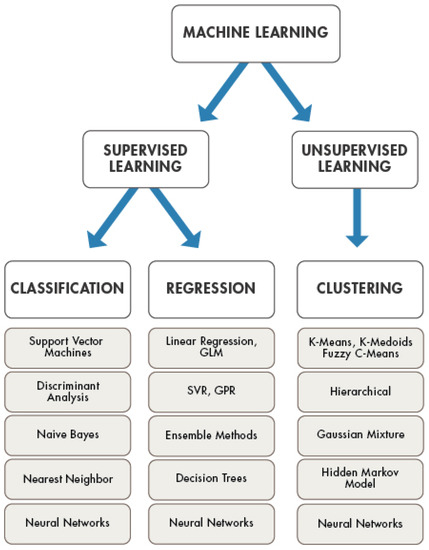
Figure 1.
Machine-learning paradigms schematization.
- -
- Classification: the outputs are divided into two or more classes, and the learning system must produce a model that assigns the unseen inputs to one or more of these. This is usually done in a supervised manner. Antispam filtering is an example of classification, where the inputs are emails and the classes are “spam” and “non-spam”.
- -
- Regression: which is also a supervised problem, the output and model used are continuous. An example of a regression is determining the amount of oil in a pipeline by having measurements of the attenuation of gamma rays passing through the pipeline. Another example is predicting the value of the exchange rate of a currency in the future, given its values in recent times.
- -
- Clustering: in which a set of inputs is divided into groups. Unlike in classification, the groups are not known beforehand, making it typically an unsupervised task.
As far as the application of the ML in the context of the algorithms of intrusion detection is concerned, reference is made to the paradigm of supervised learning and to the problem of classification. In fact, the features that will be extracted from the analyzing device of the network traffic can be pre-analyzed to decide if the observations made are relative to normal traffic or in which anomalies are present. Therefore, we speak of a “labeled” dataset, i.e., one in which the right answers for the model to learn are known (obviously only for the learning phase).
In this paper, we will refer to supervised learning, making the implicit working assumption that at least in the learning phase, the learning algorithm has the opportunity to compare the prediction with the actual response.
2.2. ML for IDS
Electronic distribution of information is becoming increasingly important, and the complexity of the data exchanged between systems is increasing at a rapid pace. Computer networks today carry all kinds of data, voice, and video traffic. Network applications require full availability without interruption or congestion. As the information systems in a company grow and develop, more networking devices are deployed, resulting in large physical ranges covered by the networked system. It is crucial that this networked system operates as effectively as possible, because downtime is both costly and an inefficient use of available resources. Network and/or protocol analysis is a range of techniques that network engineers and technicians use to study the properties of networks, including connectivity, capacity, and performance. Network analysis can be used to estimate the capacity of an existing network, look at performance characteristics, or plan for future applications and upgrades [4,5].
One of the best tools for performing network analysis is a network analyzer like Wireshark. A network analyzer is a device that gives you a very good idea of what is happening on a network by allowing you to look at the actual data that travels over it, packet by packet. A typical network analyzer understands many protocols, which enables it to display conversations taking place between hosts on a network. Wireshark can be used in this capacity.
Network analyzers typically provide the following capabilities:
- -
- Capture and decode data on a network
- -
- Analyze network activity involving specific protocols
- -
- Generate and display statistics about the network activity
- -
- Perform pattern analysis of the network activity.
Network analyzers can automatically derive a set of features that characterize network traffic [6]. This means that the network analyzer associates values to the features for each time in which the network traffic is observed. In other words, the network analyzer can be used to create a dataset that can be used in the training process of any machine-learning model. Figure 2 shows the schematic representation of essential steps in usage of ML to implement an intrusion detection algorithm.
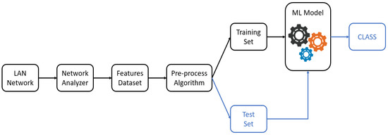
Figure 2.
Machine-learning workflow in intrusion detection.
2.3. MATLAB for Machine/Deep Learning
MATLAB is used by engineers and scientists to develop, automate, and integrate machine/deep-learning models into their domain-specific workflows. It helps them achieve this by providing:
- An open framework that supports interoperability with Python and other open-source deep-learning frameworks.
- Capabilities that extend beyond modeling to develop end-to-end applications.
- Integration and simulation of machine/deep-learning models into larger domain-specific systems.
- Dedicated support from engineers at MathWorks, developers of MATLAB.
The development efforts of MATLAB are aimed at addressing the entire system design workflow, represented in Figure 3, for building systems that rely on machine/deep learning.

Figure 3.
Workflow of AI-based project development in MATLAB.
This workflow is being applied to develop domain-specific machine/deep-learning applications in areas such as computer vision, signal processing, controls systems (reinforcement learning), image processing, automated driving, audio processing, and wireless systems.
For each of the domain’s mentioned above, MATLAB provides specialized tools and functions for data preprocessing and preparation, training interfaces, evaluation tools, and reference examples.
Having the right data is critical to the success of developing a deep-learning model but can be a time-consuming process. MATLAB provides apps for automating domain-specific labeling (signal labeler, image labeler, video labeler & audio labeler) and functions for preprocessing data, which aim at saving development time.
Users have the choice if they would like to use models developed in MATLAB, pretrained models such as GoogleNet or ResNet-50, or those available in OpenSource Frameworks TensorFlow, PyTorch or ONNX through framework interoperability. MATLAB’s deep-learning toolbox provides interactive apps that automate network design, training, and experiment management, allowing users to avoid steps that can be automated or eliminated.
Deep-learning models created in MATLAB can be integrated into system-level designs, developed in Simulink, for testing and verification using simulation. System-level simulation models can be used to verify how deep-learning models work with the overall design, and test conditions that might be difficult or expensive to test in a physical system.
These applications are being deployed to embedded and production systems through automatic code generation. Automatic code generation generates optimized native code for Intel and ARM CPUs, FPGAs, SoCs, and NVIDIA GPUs for deep networks along with preprocessing and postprocessing, eliminating errors of transcription or interpretation.
3. Related Works
This section recalls the works [7,8,9,10,11,12,13,14,15,16,17,18,19,20] from which inspiration was taken for the application of ML models and to make a comparison between the state-of-the-art results and the results achieved by the techniques we presented in the next sections.
The review in [7] intends to provide an exhaustive survey of the currently proposed ML-based intrusion detection systems to assist network intrusion detection system developers to gain a better intuition. The usefulness of this paper is to summarize the fundamental concept of ML and the intrusion detection problem, but in fact it does not present an innovative method or operational procedure of learning-model design as it is done in next sections of our paper.
The work in [8] compares different supervised algorithms for the anomaly-based detection technique. The algorithms have been applied on the KDD99 dataset, which is the benchmark dataset used for anomaly-based detection technique.
In [9], a novel supervised ML system is developed to classify network traffic whether it is malicious or benign. To find the best model considering detection success rate, a combination of a supervised learning algorithm and feature selection method has been used.
In particular, the authors present the application of an SVM (support vector machine) model compared to an artificial neural network (ANN) based on a back-propagation algorithm, applying them to the NSL–KDD dataset to which is also applied a statistical feature selection procedure.
In such works, the two models presented arrived at a final accuracy of 82% and 94% in the best cases, respectively. These results are much lower than the results achieved by the techniques proposed in this paper, especially about the result of our classifier based on k-NN, which arrives up to 99.6%.
Regarding ANN, the result of the authors in [9] is probably due to having used only “fully-connected” layers without exploiting the “batch normalization” stage, and a rather limited number of neurons for each hidden layer. It is possible to make this comparison because the NSL–KDD dataset used in [9] and our dataset (see Section 2) are organized with the same set of features and the same number of training examples.
In [10], a very detailed investigation is reported for observing several issues on the intrusive performance by using the ML classification. Here, an ML-classification algorithm is used for detecting the several categories of attacks. Furthermore, this study evaluates the performance criteria based on the feature extraction and ML-classification techniques algorithm.
In paper [11], the authors use novel feature reduction-based ML algorithms for detecting anomalous patterns in the recently provided dataset, declaring that a “high” accuracy of 86.15% has been achieved. In this paper, a comparison is presented between more classical statistical methods such as “naive Bayesian” and “logistic regression” models and ML models such as “decision tree” and “random forest”, evaluating the variation of the results as the number of features considered in a new representation space of the starting dataset is changed, reducing the number of features used down to 10.
In [11], there are reported rather mediocre results, especially about statistical methods that came to have an accuracy limited to about 75%.
In [12], a new hybrid-ML algorithm is presented that combines two existing algorithms to improve both the trained classification model performance and training time in network intrusion detection. Hybrid-ML algorithm means that multiple learning models are employed simultaneously, usually one in series with the other, so that the upstream one “helps in understanding the dataset” of the next one.
Usually this approach is used when there are no resource problems of the platforms used for the deployment of the algorithms both in terms of computing power and memory space, especially during the training phase.
In [12], the authors exploit this approach to reach an accuracy of 86.1%, which in fact is relatively low considering the type of application and compared to other works.
The authors in [13] presented the results of their experiments in evaluating the performance of detecting different types of attacks, analyzing the recognition performance by applying the random forest algorithm to the various datasets that are constructed from the Kyoto 2006+ dataset, which is the latest network packet data collected for developing intrusion detection systems.
This is the only work in which a result of comparable accuracy with the one we derived is presented, hovering around 99%. The authors decided to exploit the decision tree as a learning model, associating an Ensemble learning paradigm (random Ffrest) that has the defect of being strongly subject to the phenomenon of overfitting and has a very high computational cost with respect to a k-NN model, for example.
In the study reported in [15], an analysis was carried out by using ML approaches to determine whether the data received on the internet was normal or abnormal data. In order to achieve this goal, the KDD Cup 99 dataset, which is frequently used in literature studies, was classified by naive Bayes (NB), bayes NET (bN), random forest (RF), multlayer perception (MLP), and sequential minimal optimization (SMO) algorithms.
The intrusion detection system is used in analyzing huge traffic data; thus, an efficient classification technique is necessary to overcome the issue. This problem is considered in [16]. Well-known ML techniques, namely, SVM, random forest, and extreme learning machine (ELM), are applied.
These techniques are well-known because of their capability in classification. The NSL-knowledge discovery and data-mining dataset was used, which is considered a benchmark in the evaluation of intrusion detection mechanisms. The results indicated that ELM outperforms other approaches.
In [17] by using k-means clustering algorithm and an alternative method of support vector machine classification algorithm, it can automatically construct the distribution of normal packet payload and detect its deviation. Furthermore, the method proposed by the authors showed that the proposed hybrid algorithm provides significantly more detection accuracy than the most used open-source Snort system.
The authors of [18] presented a method which integrated a clustering algorithm with support vector machine to improve the accuracy and recognition rate of IDS. Firstly, the preprocessed data was processed by clustering algorithm and divided into several subsets, and then ML algorithm was used to model each subset.
In [19], the authors analyzed the advantages and disadvantages of the existing intrusion detection algorithm, focused on the in-depth study of the intrusion data feature based on deep learning, proposed a new feature selection method, conducted experiments with the special dataset of intrusion detection, and verified the scientific support and practicability of the theoretical method through full comparative experiments and parameter analysis.
In [20], the performances of some supervised (i.e., KNN and SVM) and unsupervised (i.e., isolation forest and k-means) algorithms were evaluated for intrusion detection, using dataset UNSW-NB12.
The research presented in [21] was focused on the evaluation of characteristics for different well-established machine-leaning algorithms commonly applied to IDS scenarios. To do this, a categorization for cybersecurity datasets into several groups was first considered. Making use of this division, [21] sought to determine which neural network model (multilayer or recurrent), activation function, and learning algorithm yielded higher accuracy values, depending on the group of data.
The work presented in [22] provides an interactive method of visualizing network intrusion detection data in three-dimensions. The objective was to facilitate the understanding of network-intrusion-detection data using a visual representation to reflect the geometric relationship between various categories of network traffic. This interactive visual representation can potentially provide useful insights to aid the understanding of machine learning results.
The survey in [23] comprehensively reviews and compares the key previous deep learning-focused cybersecurity surveys. Through an extensive review, this survey provides a novel fine-grained taxonomy that categorizes the current state-of-the-art deep learning-based IDSs with respect to different facets, including input data, detection, deployment, and evaluation strategies.
In general, the problem with the works mentioned above is the absolute accuracy of the algorithms, which is around 85% on average. This value is unacceptable in applications where a high rate of security of systems under attack is required, such as the military defense field, which is instead referred to in the work developed in this paper.
4. Use Case Dataset Analysis and Preprocessing
4.1. Dataset Analysis and Managing
The dataset [24] to be audited was provided, consisting of a wide variety of intrusions simulated in a defense-network environment. It created an environment to acquire raw TCP/IP dump data for a network by simulating a typical US Air Force LAN, as shown in Figure 3. This case study has been selected as being representative of a safety-critical networked application.
The features which composed the used dataset with a brief description of the meaning of each one are reported below. In this sense, the dataset used in this work is organized as the more commonly used KDD-99 dataset. The main difference is that our dataset it is representative of military scenario, meanwhile the commonly used dataset are related with classic LAN from a non-safety-critical application.
Table 1 provides the list of features of the used dataset with a short description, dividing features in terms of “Basic”, “Content-based”, “Time-based” and “Connection-based”. Table 1 also details if the reported feature is a “Continuous” (C) or “Discrete” (D) one.

Table 1.
Features Description.
The LAN topology is Figure 4 in [24] was representative of a real distributed control system for defense applications and was blasted with multiple attacks. A connection is a sequence of TCP packets between a source IP address and a target IP address under some well-defined protocol. The sequence of TCP packets is starting and ending at some specific time deadlines, between which the data flows. Also, each connection is labeled as either normal or as an attack with exactly one specific attack type. Each connection record in [24] consists of about 100 bytes. For each TCP/IP connection, 41 quantitative and qualitative features are obtained from normal and attack data (3 qualitative and 38 quantitative features). The class variable has two categories: Normal and Anomalous.
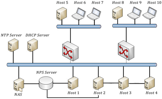
Figure 4.
Network-topology schematization of the considered case study.
To be able to use the dataset, it is also necessary to convert the features that assume categorical values into alternative features that assume numerical values. A possible choice, which besides being the most used is also the one adopted in this work, is that of “dummy” variables [25]. The concept of dummy variables is schematized in the Figure 4.
Each column of d in Figure 5 represents one of the categories in c. Each row corresponds to an observation and has one element with value 1 and all other elements equal to 0. The 1 appears in the column corresponding to that observation’s assigned category.
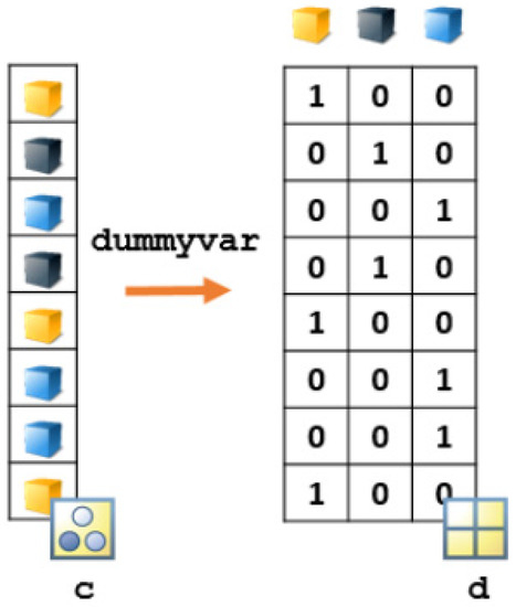
Figure 5.
Network-topology schematization.
Upon visual inspection, some columns of the dataset consist of many zeroes, and some features take on significantly larger values than others. To avoid these distortion effects from affecting the classification process using one of the chosen learning models, another preliminary operation is to apply normalization to the columns of the dataset. Some features have a “very small” variability, which returns downstream of normalization many NaNs (not-a-number). This happens in when the transformation is applied. Therefore, for columns in the dataset with small variance, the calculator interprets division by a very small number as a NaN. It can be assumed that the columns of the dataset that have many NaNs have little information content and can therefore be eliminated.
4.2. Multidimensional-Scaling Analysis
Multidimensional scaling (MDS) is a set of techniques for projecting points from a multidimensional space into a space of lower dimension [26]. The aim is to try to reproduce as much as possible the distances between the original points but in a space of reduced dimension. The input for MDS is “proximity data”, i.e., the observed similarities or dissimilarities between all pairs of observations.
The proximity matrix is usually visualized as a lower triangular matrix of non-negative values, with the implicit idea that the values on the diagonal are all zero and that the upper triangular part of the matrix is a mirror image of the lower triangular part (i.e., the matrix is symmetrical).
The general MDS problem can be specified, in its essence, as follows: given a matrix of proximity between objects (i.e., observations or variables), one wants to reconstruct the original map as precisely as possible. Another aspect of the problem is that the number of dimensions in which the given entities are to be projected is not known a priori. Consequently, determining the number of dimensions is another problem to be solved. The operating procedure for deriving the matrix representing the data in the reduced space of the new features is given below [27].
The feature matrix , where is the number of accumulated observations and is the number of features extracted from each observation, can be written as follows, where represents the value that the feature takes on at the observation.
The “similarity” matrix is constructed, defined through the choice of metric (which then defines the measure of similarity between observations in the dataset, i.e., between the rows of X). Usually the Euclidean distance or the cosine of similarity are chosen. Equation (2) shows the formal definition of the two metrics and
where . Then the general element of the similarity matrix can be written as . Let define the “double centering” matrix as in Equation (3):
with and apply a congruence transformation to the matrix , defining the new “barycenter” matrix . The eigenvalues are calculated, selecting those with the highest value , with the new number of features, and the eigenvectors of B relative to the selected eigenvalues are calculated.
is defined as the base change matrix.
The matrix that represents the data in the new features space can be calculated as , where .
The results obtained with both the choice of Euclidean distance, equivalent to Principal Component Analysis (PCA), and cosine of similarity were compared.
With the dataset is reduced to seven new features with which about 85% of the initial information content described, while with it is reduced to five features in the new feature space with more than 93% of the information content described, as shown in Figure 6.
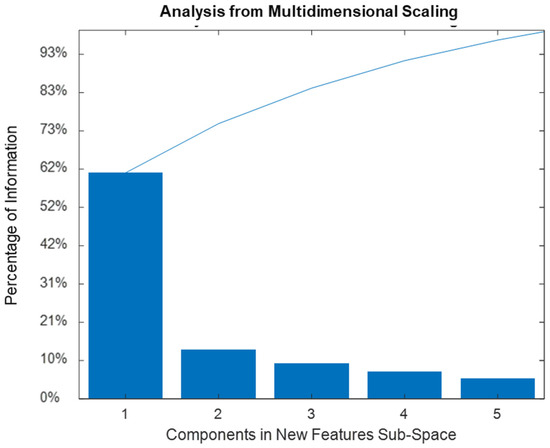
Figure 6.
Pareto plot of the percentage of information per each new space features component.
It should be noted that the articles in the Related Works section adopt methods that are computationally heavy, as they require recursive procedures such as wrapper filtering. Instead, this work applies a direct method of construction of the base change in the new feature space, choosing as metric of comparison between the columns of the dataset the cosine of similarity, which, as mentioned above, gives results much better than the Euclidean distance and the PCA.
4.3. Performance Analysis
In this work we present the development of classification models for a binary classification problem with an application to intrusion detection systems. In binary classification problem, if P (positive) and N (negative) are the possible labels/classes for each observation, a classification model can produce only four results, see Figure 7:
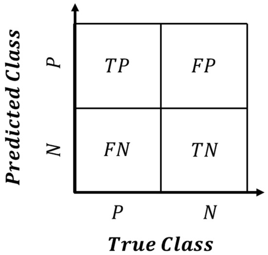
Figure 7.
Representation of classification model result in confusion matrix.
- TP (true positive): if the model predicts P, and it is also the correct answer.
- FP (false positive): if the model predicts P, but the correct answer is N.
- TN (true negative): if the model predicts N, and it is also the correct answer.
- FN (false negative): if the model predicts N, but the correct answer is P.
In this way, it is possible to define a useful representation called contingency or confusion matrix, that is basically a table in which the results of classification model predictions are collected.
From this representation of the prediction result by the classification model, it is possible to define some useful index to evaluate the model itself in terms of quality in classifying ability. In particular, the most used index in practice are the following described:
- Sensitivity or true-positive rate (TPR) it is defined as which represents the number of predicted P with respect to the total P in the dataset.
- Specificity or true-negative rate (TNR) it is defined as which represents the number of predicted N with respect to the total N in the dataset.
- Precision or positive-predictive value (PPV) is defined as which is the number of correct prediction about P with respect to the total number of predicted P.
- Accuracy (ACC) that is defined as and represents the total number of correct answer by the model with respect to the total number of observation in the dataset.
Intuitively, the usage of only accuracy as an estimation of the performance is not correct from a conceptual point of view. Since the accuracy merges the result in the ability of the model to correctly predict both P and N, it is not possible to evaluate if the model is better at correctly predicting P or N.
Basically, a high value of accuracy can derive by very good ability of the model to correctly predict only one of the possible classes. From this simple consideration when a model performance is evaluated, the other indexes of quality are also required. Furthermore, those considerations are very useful for comparing different models of classifier, since different models can be able to predict very different classes but with similar accuracy.
It depends on the final application, but this can be useful if one of the classes is more “relevant” to correctly predict with respect to the other one. For example, in intrusion detection systems, it is intuitive that it is more important to correctly predict the observation related with the “anomaly” label compared to the “normal” one.
In the final analysis of each proposed model, we report a table to compare the classification result with respect to the above-described coefficients. In every section in which a different model is presented, the results are summarized in terms of confusion matrix, and in the case of the ANN classifier, the training loss and accuracy functions behavior are also shown.
5. Design of Machine-Learning-Based Classifiers
5.1. K-Nearest Neighbors Classifier
The k-nearest neighbors (k-NN) is an algorithm used in pattern recognition for classifying objects based on the characteristics of objects close to the one under consideration [3]. In k-NN classification, the output is a class membership. An object is classified by a plurality vote of its neighbors, with the object assigned to the most common class among its k-nearest neighbors (k is a positive integer, typically small). If , the object is simply assigned to the class of that single nearest neighbor. The k-value in the k-NN algorithm determines the number of training data points that are to be considered while determining the class of the test data points. The essential steps to implement a k-NN classifier are as follows:
- Starting from the training dataset matrix , with which a categorical vector of the classes to which each accumulated observation belongs is associated.
- Each observation can be represented by a vector whose components are relative to the values assumed by the features. In essence, each row of is a “sample vector” to which a class is associated.
- Once a metric has been chosen, typically the Euclidean norm, the distances between the new observation and those in the dataset are calculated.
- The vector of pairs ( distance from , class) is then constructed, . By sorting according to the distances in an increasing way and fixing the value of the parameter k, the first k classes are selected, and a majority policy is applied to decide which class the new observation belongs to.
Noticeably in the k-NN technique, the truly learning phase is not present, because the training set is composed by the accumulated observations, which are compared every time with the new ones.
In the case below, the best result was obtained for k = 1, see Figure 8, comparing in terms of total accuracy the cases for k = 1,2,3,4,5,10,20,40,100, and 200 following the classic heuristic choice, for which k must be a relatively small number compared to the size of the dataset. As expected, for a value of k that is “too large”, k the performance of the algorithm degrades. This phenomenon in the presented case occurs for k > 5. By contrast, for increasing k in the range , where we would expect that the increase of k increases the performance, in reality for k = 1,2,3,4, and 5, we obtain substantially equivalent performance (k is reported as the best in any case). This phenomenon can be assigned to the intrinsic structure of the dataset, in which probably, even if perfectly balanced between the two possible categories (normal or anomaly), the structure of the observations is highly repetitive.
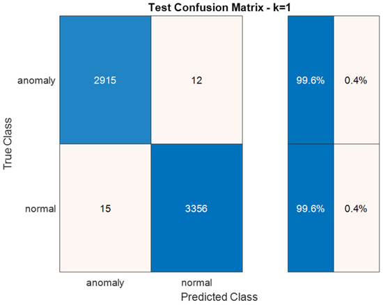
Figure 8.
Best confusion matrix obtained on test set with K-NN classifier.
Furthermore, it has been verified that the choice of metric is practically irrelevant to the total accuracy, having compared test results of K-NN models with both distance and cosine similarity metrics. This can be attributed to the fact that in the feature space, points that belong to a class in addition to being condensed on domains at different distances from the origin, also have a substantially different average orientation of the pointing vectors. This peculiarity is obviously not modified in the initial manipulation of the dataset through the algebraic transformations in the space of reduced dimension features.
5.2. Artificial Neural Network Classifier
We can consider an artificial neural network (ANN) as a “black box” algorithm, with inputs, intermediate layers in which happens the real “learning” phase, and outputs that consists of the result. The neural network is composed of “units” called neurons, arranged in successive layers. Each neuron is typically connected to all neurons in the next layer via weighted connections. A connection is nothing more than a numerical value (the “weight”), which is multiplied by the value of the connected neuron.
Each neuron, as schematically represented in Figure 9, sums the weighted values of all the neurons connected to it and adds a bias value. An “activation function” is applied to this result, which does nothing more than mathematically transform the value before passing it to the next layer.
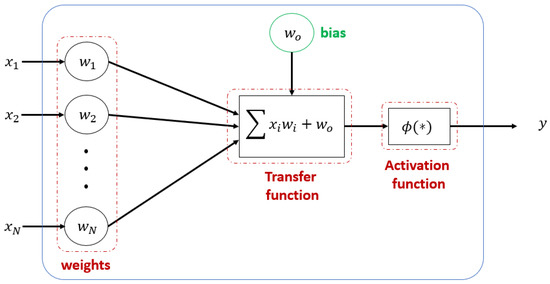
Figure 9.
Artificial neuron architecture.
In this way, the input values are propagated through the network to the output neurons, which is practically all that a neural network does. The goal of the training phase is to adjust weights and bias to get the desired result. For this purpose, there are different techniques. Neural network learning is based on the algorithm of updating the weights of neurons. The update algorithms are basically based on gradient descent. Once an objective function is set, during the learning phase the neuron weights will re-arrange to minimize that function.
Many network architectures have been elaborated. In this work, for IDS, we refer to the architecture represented in Figure 10, which identifies a feed-forward neural network [28]. In the neural network of Figure 10, the fully connected layers admit only connections with the neurons of the previous and following layers and not between neurons of the same layer. The training options used in this work are the SGDM (stochastic gradient descent with momentum) algorithm, initial learning rate of 0.0001, and loss function MSE (mean squared error).
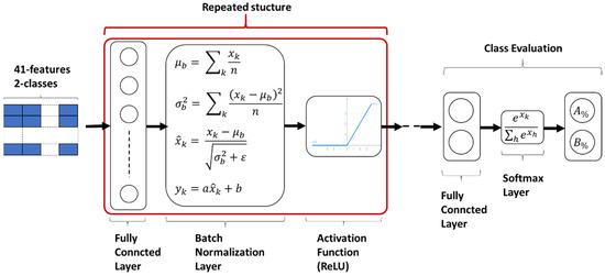
Figure 10.
Base architecture of used artificial neural network.
The essential formulation of the SGDM (stochastic gradient descent with momentum) algorithm is given in Equation (4), where is the learning rate and is the convex combination coefficient such that .
SGDM is a method which helps accelerating gradient vectors in the right directions, thus leading to a faster convergence. SGDM is one of the most popular optimization algorithms and many state-of-the-art ANN models are trained using it. Momentum is a physical property that enables a particular object with mass to continue in its trajectory even when an external opposing force is applied, which means overshoot. For example, one speeds up a car and then suddenly hits the brakes, the car will skid and stop after a short distance, overshooting the mark on the ground. The same concept applies to neural networks, during training, the update direction tends to resist change when momentum is added to the update scheme.
When the neural net approaches a shallow local minimum it is like applying brakes but not enough to instantly affect the update direction and magnitude. Hence the neural nets trained this way will overshoot past smaller local minima points and only stop in a deeper global minimum. Thus, momentum in neural nets helps them get out of local minima points so that a more important global minimum can be found. Too much momentum may create issues as well as systems that are not stable, which may create oscillations that grow in magnitude. In such cases, one needs to add decay terms and so on. It is just physics applied to neural net training or numerical optimizations.
Four different models based on the structure presented in Figure 11 were compared, differing in the number of neurons in each of the fully connected layers and in the number of times the common structure is repeated. Note that in the case of the neural network used, as shown in the figures above, all 41 features are passed as input. This defines a middle ground between classical machine learning and deep learning, where the network is also used to fulfil the task of feature extraction from the raw data [29]. In the considered case used in Section 4.1, the network analyzer provides structured measures, already organized in features, that are useful to fully exploit the potentialities of learning models based on artificial neural networks. Therefore, the models tested in this work use all the 41 features of the considered case study in Section 4.1, without exploiting the process of feature space reduction described in Section 4.2 that instead was useful to reduce the computational cost associated to the K-NN classifier design in Section 5.1.
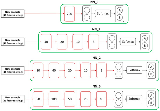
Figure 11.
Different artificial neural networks compared.
Figure 12 and Figure 13 show the trends (average mean value) of the loss function and of the accuracy, during the phase of training, for each of the four nets (NN0, NN1, NN2, and NN3 in Figure 11) tested. Figure 14 and Figure 15 show training loss and accuracy functions.
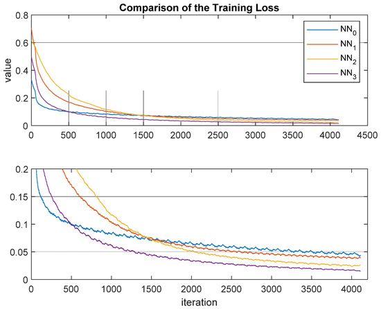
Figure 12.
Loss-function behaviors comparison during training phase.
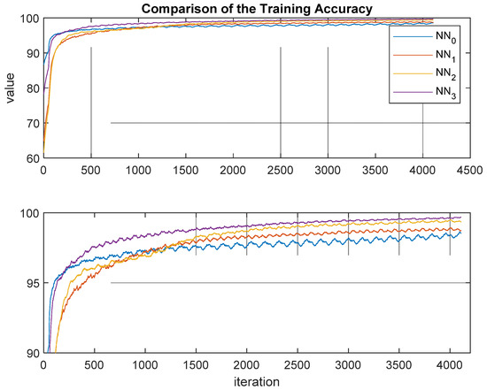
Figure 13.
Accuracy behaviors comparison during training phase.
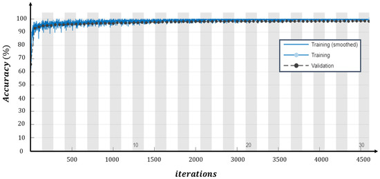
Figure 14.
Training progress with respect to accuracy function.
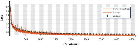
Figure 15.
Training progress with respect to loss function.
The best result is obtained by , whose confusion matrix is shown in Figure 16. The results are comparable with those obtained with the k-NN classifier designed in Section 5.1.
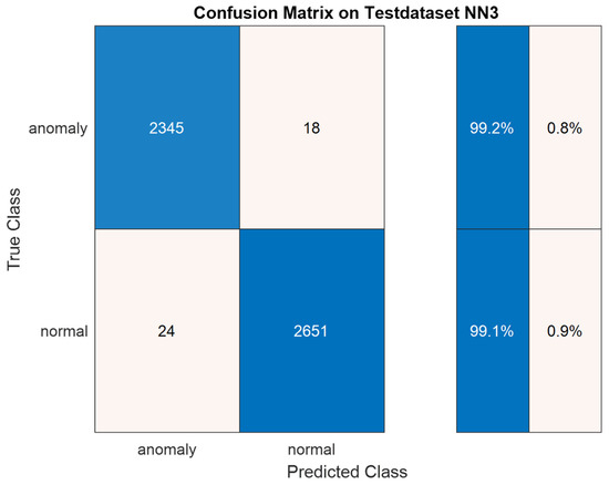
Figure 16.
Best confusion matrix obtained on test set with ANN classifier (NN3).
5.3. Models Comparison
In the following we summarize in table form, see Table 2, the obtained results, comparing the k-NN and ANN with respect to the classic statistical index previously described.

Table 2.
Summary of the obtained results.
The models are basically equivalent in terms of absolute ability to correctly classify the observation from the test set, with each index of interest over a value of 99%. In this particular case used, the KNN classifier sims a little bit better than the trained ANN. This can be due both to the specific dataset organization and to the size of the used ANN, which in any case, in respect to the more commonly used, it is a “small” feedforward neural network.
In machine-learning theory, there are more models to use to face classification problems. In this work we choose the K-NN models because of its specific advantage in simplicity and interpretability, which can be summarized as follows:
- it does not learn anything in the training period. It does not derive any discriminative function from the training data. In other words, there is no training period for it. It stores the training dataset and learns from it only at the time of making real-time predictions. This makes the KNN algorithm much faster than other algorithms that require training, e.g., SVM, linear regression etc.
- since the KNN algorithm requires no training before making predictions, new data can be added seamlessly which will not impact the accuracy of the algorithm.
- KNN is very easy to implement. There are only two parameters required to implement KNN, i.e., the value of k and the distance function (e.g., Euclidean or Manhattan, etc.)
Clearly, there are also some disadvantages, related to the number of features in the data representation. In large datasets, the cost of calculating the distance between the new point and each existing point is huge, which degrades the performance of the algorithm. In our work, in fact, a features reduction/selection procedure is presented to avoid any problems related with data dimensionality.
The other model we propose to fit the data and predict anomaly in network traffic is a feedforward artificial neural network, with specific structure described in the previous section. The usage of an ANN instead of more complex architecture such as CNN (convolutional neural network) or RNN (recursive neural network) is related to the application itself, since the collected observation can be organized in tabular dataset and each observation comes from the analysis of a network sniffer, which in general directly provides a set of statistical features from the communication traffic. In machine/deep-learning practice it is suggested to use ANN with a tabular dataset, CNN with an images dataset, and RNN with a sequence dataset. This means that for intrusion detection systems, it is not required, and probably not appropriate, to apply more complex architecture such as RNN or CNN. ANNs also have a higher-fault robustness ability with respect to other architecture, providing the capability to work with also incomplete data. Furthermore, due to the higher complexity, CNN and RNN suffer from the problem of gradient vanishing/exploding, and the obtained results are less interpretable compared to ANN ones.
6. Conclusions
Two machine-learning methods for anomaly classification in intrusion detection systems have been presented and compared on the same dataset representing the data traffic of a LAN for defense applications.
A feature reduction method based on multidimensional scaling has been also exploited, highlighting that the choice of cosine of similarity as a metric for comparing the observations that form the training set gives better results than PCA, where the metric is the Euclidean distance in the feature space.
The classification results have been presented in terms of confusion matrices that highlight that the two methods, in absolute terms of final accuracy, which are practically equivalent. However, in the specific case of the dataset under consideration, K-NN proved to be slightly better, both in the classification of the anomaly class and in the normal class.
The results presented are related to the use of K-NN after the procedure of reduction of the space of the features, in order to be sure to avoid overfitting phenomena and that then the results obtained in the testing phase are generalizable to other future observations obtained with a network analyzer, provided obviously that the features that are extrapolated in an automatic way are the initial 41.
For use of the ANN instead, a mixed approach between the classic machine learning and the deep learning was followed. However, the network is left to learn which of the 41 initial features are representative of all the information contained in the dataset. Since the data extracted by the network analyzer is already organized in the form of both quantitative and qualitative features, it is probably not formally legitimate to speak of real deep learning.
It should also be noted that the results of the application of the methods presented here have been obtained on a dataset which is representative of a realistic scenario of concrete interest in terms of application, such as a defense application (US Air Force LAN).
Author Contributions
Conceptualization, S.S. and P.D.; methodology, S.S. and P.D.; software, P.D.; validation S.S. and P.D.; writing—original draft preparation, S.S. and P.D.; writing—review and editing, S.S. and P.D. All authors have read and agreed to the published version of the manuscript.
Funding
This work was funded by MIUR through project Dipartimenti di Eccellenza Crosslab.
Conflicts of Interest
The authors declare no conflict of interest.
References
- Nandita, S.; Sil, J. Intrusion Detection: A Data Mining Approach; Springer: Singapore, 2020. [Google Scholar]
- Mello, R.F.; Ponti, M.A. Machine Learning: A Practical Approach on the Statistical Learning Theory; Springer: Berlin/Heidelberg, Germany, 2018. [Google Scholar]
- Christoph, M. Interpretable Machine Learning; Lulu. com: Cedar Fork, NC, USA, 2020. [Google Scholar]
- Clarence, C.; Freeman, D. Machine Learning and Security: Protecting Systems with Data and Algorithms; O’Reilly Media, Inc.: Sebastopol, CA, USA, 2018. [Google Scholar]
- Mamoun, A.; Tang, M.J. (Eds.) Deep Learning Applications for Cyber Security; Springer: Berlin/Heidelberg, Germany, 2019. [Google Scholar]
- Monowar, H.B.; Bhattacharyya, D.K.; Kalita, J.K. Network Traffic Anomaly Detection and Prevention: Concepts, Techniques, and Tools; Springer: Berlin/Heidelberg, Germany, 2017. [Google Scholar]
- Phadke, A.; Kulkarni, M.; Bhawalkar, P.; Bhattad, R. A Review of Machine Learning Methodologies for Network Intrusion Detection. In Proceedings of the 2019 3rd International Conference on Computing Methodologies and Communication (ICCMC), Erode, India, 27–29 March 2019. [Google Scholar]
- Tahir, M.; Rais, H.B. Machine learning algorithms in context of intrusion detection. In Proceedings of the 2016 3rd International Conference on Computer and Information Sciences (ICCOINS), Kuala Lumpur, Malaysia, 15–17 August 2016. [Google Scholar]
- Taher, K.A.; Jisan, B.M.Y.; Rahman, M. Network intrusion detection using supervised machine learning technique with feature selection. In Proceedings of the 2019 International Conference on Robotics, Electrical and Signal Processing Techniques (ICREST), Dhaka, Bangladesh, 10–12 January 2019. [Google Scholar]
- Illavarason, P.; Sundaram, B.K. A Study of Intrusion Detection System using Machine Learning Classification Algorithm based on different feature selection approach. In Proceedings of the 2019 Third International conference on I-SMAC (IoT in Social, Mobile, Analytics and Cloud) (I-SMAC), Palladam, India, 12–14 December 2019. [Google Scholar]
- Srivastava, A.; Agarwal, A.; Kaur, G. Novel Machine Learning Technique for Intrusion Detection in Recent Network-based Attacks. In Proceedings of the 2019 4th International Conference on Information Systems and Computer Networks (ISCON), Mathura, India, 21–22 November 2019. [Google Scholar]
- Chuang, P.-J.; Li, S.-H. Network Intrusion Detection using Hybrid Machine Learning. In Proceedings of the 2019 International Conference on Fuzzy Theory and Its Applications (iFUZZY), New Taipei City, Taiwan, 7–10 November 2019. [Google Scholar]
- Park, K.; Song, Y.; Cheong, Y.-G. Classification of attack types for intrusion detection systems using a machine learning algorithm. In Proceedings of the 2018 IEEE Fourth International Conference on Big Data Computing Service and Applications (BigDataService), Bamberg, Germany, 26–29 March 2018. [Google Scholar]
- Kaya, Ç.; Oktay, Y.; Sinan, A. Performance analysis of machine learning techniques in intrusion detection. In Proceedings of the 2016 24th Signal Processing and Communication Application Conference (SIU), Zonguldak, Turkey, 16–19 May 2016. [Google Scholar]
- Ertam, F.; Llhan, F.K.; Orhan, Y. Intrusion detection in computer networks via machine learning algorithms. In Proceedings of the 2017 International Artificial Intelligence and Data Processing Symposium (IDAP), Malatya, Turkey, 16–17 September 2017. [Google Scholar]
- Ahmad, I.; Basheri, M.; Iqbal, M.J.; Rahim, A. Performance comparison of support vector machine, random forest, and extreme learning machine for intrusion detection. IEEE Access 2018, 6, 33789–33795. [Google Scholar] [CrossRef]
- Zhang, H.; Lin, K.-Y.; Chen, W.; Li, G. Using Machine Learning techniques to improve Intrusion Detection Accuracy. In Proceedings of the 2019 IEEE 2nd International Conference on Knowledge Innovation and Invention (ICKII), Seoul, Korea, 12–15 July 2019. [Google Scholar]
- Liang, D.; Liu, Q.; Zhao, B.; Zhu, Z.; Liu, D. A Clustering-SVM Ensemble Method for Intrusion Detection System. In Proceedings of the 2019 8th International Symposium on Next Generation Electronics (ISNE), Zhengzhou, China, 9–10 October 2019. [Google Scholar]
- Xin, M.; Wang, Y. Research on Feature Selection of Intrusion Detection Based on Deep Learning. In Proceedings of the 2020 International Wireless Communications and Mobile Computing (IWCMC), Limassol, Cyprus, 15–19 June 2020. [Google Scholar]
- Portela, F.G.; Mendoza, F.A.; Benavides, L.C. Evaluation of the performance of supervised and unsupervised Machine learning techniques for intrusion detection. In Proceedings of the 2019 IEEE International Conference on Applied Science and Advanced Technology (iCASAT), Queretaro, Mexico, 27–28 November 2019. [Google Scholar]
- Larriva-Novo, X.; Vega-Barbas, M.; Villagrá, V.A.; Rodrigo, M.S. Evaluation of cybersecurity data set characteristics for their applicability to neural networks algorithms detecting cybersecurity anomalies. IEEE Access 2020, 8, 9005–9014. [Google Scholar] [CrossRef]
- Zong, W.; Chow, Y.-W.; Susilo, W. Interactive three-dimensional visualization of network intrusion detection data for machine learning. Future Gener. Comput. Syst. 2020, 102, 292–306. [Google Scholar] [CrossRef]
- Aldweesh, A.; Derhab, A.; Emam, A.Z. Deep learning approaches for anomaly-based intrusion detection systems: A survey, taxonomy, and open issues. Knowl. Based Syst. 2020, 189, 105124. [Google Scholar] [CrossRef]
- Available online: https://www.kaggle.com/sampadab17/network-intrusion-detection?select=Train_data.csv (accessed on 1 February 2021).
- Bruce, P.; Bruce, A.; Gedeck, P. Practical Statistics for Data Scientists: 50+ Essential Concepts Using R and Python; O’Reilly Media: Sebastopol, CA, USA, 2020. [Google Scholar]
- Tan, P.-N.; Steinbach, M.; Kumar, V. Introduction to Data Mining; Pearson Education India: Tamil Nadu, India, 2016. [Google Scholar]
- Frank, E.; Mark, A.H.; Ian, H. Witten. In Online Appendix for Data Mining: Practical Machine Learning Tools and Techniques; The WEKA Workbench: Hamilton, New Zealand, 2016. [Google Scholar]
- Aggarwal, C.C. Neural Networks and Deep Learning; Springer: Berlin/Heidelberg, Germany, 2018. [Google Scholar]
- Mark, R. Deep Learning with Structured Data; Manning Publications: Shelter Island, NY, USA, 2020. [Google Scholar]
Publisher’s Note: MDPI stays neutral with regard to jurisdictional claims in published maps and institutional affiliations. |
© 2021 by the authors. Licensee MDPI, Basel, Switzerland. This article is an open access article distributed under the terms and conditions of the Creative Commons Attribution (CC BY) license (http://creativecommons.org/licenses/by/4.0/).