Article

A Novel Deep Learning Backstepping Controller-Based Digital Twins Technology for Pitch Angle Control of Variable Speed Wind Turbine

by
Ahmad Parvaresh
1,
Saber Abrazeh
2,
Saeid-Reza Mohseni
3,
Meisam Jahanshahi Zeitouni
4,
Meysam Gheisarnejad
5 and
Mohammad-Hassan Khooban
6,*
1
Electrical Engineering Department, Shahid Bahonar University of Kerman, Kerman 76169-14111, Iran
2
School of Electrical & Computer Engineering, Shiraz University, Shiraz 71946-84334, Iran
3
Electrical Engineering Department, Sharif University of Technology, Tehran 11365-11155, Iran
4
Electrical & Electronic Engineering Department, Shiraz University of Technology, Shiraz 71557-13876, Iran
5
Department of Electrical Engineering, Islamic Azad University, Najafabad Branch, Najafabad, Esfahan 8514143131, Iran
6
DIGIT, Department of Engineering, Aarhus University, 8200 Aarhus N, Denmark
*
Author to whom correspondence should be addressed.
Designs 2020, 4(2), 15; https://doi.org/10.3390/designs4020015
Submission received: 17 April 2020 / Revised: 31 May 2020 / Accepted: 5 June 2020 / Published: 22 June 2020

Abstract

:
This paper proposes a deep deterministic policy gradient (DDPG) based nonlinear integral backstepping (NIB) in combination with model free control (MFC) for pitch angle control of variable speed wind turbine. In particular, the controller has been presented as a digital twin (DT) concept, which is an increasingly growing method in a variety of applications. In DDPG-NIB-MFC, the pitch angle is considered as the control input that depends on the optimal rotor speed, which is usually derived from effective wind speed. The system stability according to the Lyapunov theory can be achieved by the recursive nature of the backstepping theory and the integral action has been used to compensate for the steady-state error. Moreover, due to the nonlinear characteristics of wind turbines, the MFC aims to handle the un-modeled system dynamics and disturbances. The DDPG algorithm with actor-critic structure has been added in the proposed control structure to efficiently and adaptively tune the controller parameters embedded in the NIB controller. Under this effort, a digital twin of a presented controller is defined as a real-time and probabilistic model which is implemented on the digital signal processor (DSP) computing device. To ensure the performance of the proposed approach and output behavior of the system, software-in-loop (SIL) and hardware-in-loop (HIL) testing procedures have been considered. From the simulation and implementation outcomes, it can be concluded that the proposed backstepping controller based DDPG is more effective, robust, and adaptive than the backstepping and proportional-integral (PI) controllers optimized by particle swarm optimization (PSO) in the presence of uncertainties and disturbances.

1. Introduction and Preliminaries

Nowadays, renewable energy sources have been playing a significant role in the achievement of reliable, efficient and affordable energy and they have good business development prospects. In a comparison to these energy sources, wind energy is one of the fastest growing, economically cost-effective and most promising energy sources, and its development has progressed tremendously worldwide. Generally, the kinetic energy conversion of the wind into the electrical energy is done by wind turbine (WT). The operating region of every WT is mainly classified into two key areas: below and above-rated wind speed. The control objective at below-rated wind speed is to capture the maximum available power from the wind flow, using variable speed operation of WT. The pitch angle control is used to maintain the rated power at above-rated wind speed, while minimizing the load stress on the drive-train shaft at the same time [1]. Although the majority of WTs are fixed speed, numerous variable speed WTs are being increased because of this fact that they maximize the energy capture by functioning turbine at the maximum power coefficient.
A wide range of classical and modern control methods have been suggested to design pitch angle controllers at above-rated wind speed [2,3,4]. As highly sophisticated technologies, modern controllers can also increase the efficiency and performance of WTs, while keeping maintenance costs low [5,6]. In the last decades, the backstepping control strategy has been amply investigated and developed to access the stability goal of the whole system and state estimation obstacles. This control technique suggests good performance in both steady-state and transient operations, even in the presence of uncertainties, parameter variations, and load torque disturbances. The backstepping control laws are easily constructed and associated with Lyapunov functions [7,8]. Nonlinear integral backstepping (NIB), due to its recursive nature is the completely efficient controller, showed a great deal in stabilizing the nonlinear fixed-model WT systems with the presence of perturbations, and besides the integral action has been used to compensate the steady-state error [9]. On the other hand, 1111nonlinear characteristics of WTs lead to tough and almost impossible efforts to extract an exact model of a system. Furthermore, plant dynamics can be intensively changed with output disturbances, therefore we have no way to go through model-free controllers (MFCs). M. Fliess and C. Join in [10] have proposed an accurate definition of the MFC technique and its application in nonlinear systems to compensate modeling error.
Another key issue in NIBs is tuning its parameters to achieve the best outputs from the controller actions. Numerous studies have been done to find suitable optimization algorithms that are applicable to wind power generation systems [11,12]. Among other types of optimization and tuning methods, reinforcement learning (RL) has been increasingly developing [13]. There are lots of different online model-free value-function-based RL algorithms that use the deducted future reward criterion. Q learning [14], state–action–reward–state–action (SARSA) [15,16], and Actor-Critic (AC) methods [17] are well known, and there are also two more recent algorithms: QV learning [18] and AC learning automaton (ACLA) [18]. Furthermore, many policy search and policy gradient algorithms have been proposed [19,20], and there exist model-based [21] and batch RL algorithms [22]. Recently, the deep deterministic policy gradients (DDPG) algorithm has been widely using in a plethora of applications because of its strong learning ability and stability [23]. In this algorithm, there are two major neural networks (NNs): an actor NN (ANN) and a critic network (CNN). ANN is used to approximate the policy function and CNN is used to approximate the value function and besides, it works on approximation with deep neural networks for both the action-value function and the policy [24].
One of the newest concepts of information technology is known by digital twin (DT), which is increasingly applied in wind energy conversion systems. The term digital twin “means an integrated multi-physics, multi-scale, probabilistic simulation of a complex product, which functions to mirror the life of its corresponding twin” [25]. The combination of physical and virtual data has many advantages. On one hand, the physical product can be made more intelligent to actively adjust its real-time behavior according to the recommendations made by the virtual product. On the other hand, the virtual product can be made more factual to accurately reflect the real-world state of the physical product [26]. Nevertheless, we gathered evidence during our research that digital twin in a wind turbine is still in the early stages of development. A new concept of a digital twin has been considered in this paper. Firstly, two separate tests, software-in-loop (SIL) and hardware-in-loop (HIL), have been considered to show the abilities of the controller in real-time applications. Secondly, with a unique combination of these tests, it has been shown a new concept of digital twin, which is clearly efficient and effective.
In this paper, a new DDPG-based NIB-MPC controller has been proposed, to achieve the aforementioned key points for the promotion of pitch angle control of a variable speed wind turbine in above-rated wind speed. The parameters of the proposed controller have been tuned adaptively by the DDPG algorithm with the actor-critic structure. In this controller, there is no need for a system dynamics model and the system uncertainties have been estimated by ultra-local model and compensated via feedback signal. In NIB-MPC structure, NIB gains have been chosen as control parameters and then they have tuned adaptively by the DDPG algorithm. To highlight the capabilities of the proposed approach and achievement of similarity between output behavior of the system in software-in-loop (SIL) and hardware-in-loop (HIL) testing, a digital twin (DT) of proposed controller has been presented. This DT is implemented with presenting a novel strategy, on a TI digital signal processor (DSP) computing device.
This paper is organized as follows. Section 2 presents the nonlinear model of the variable speed wind turbine. Then, Section 3 introduces the proposed controller with detail. Section 4 focuses on the digital twin concept for implementing of the proposed controller and its SIL and HIL testing. The results of simulation in the Matlab/Simulink platform and also the implementation of the controller on TI DSP hardware has been presented in Section 5. Finally, Section 6 summarizes the main contributions and describes some additional avenues for continuing research.

2. Variable Speed Wind Turbine Nonlinear Model

As well known, wind energy is electricity produced by using mechanical components and electrical generators. A two-mass model is commonly used in the literature [27] to describe the variable speed wind turbine nonlinear dynamics. The use of a two-mass model is motivated due to this fact that the control laws derived from this model are more general and can be applied for wind turbines of different sizes. Particularly, these controllers are more adapted for high-flexibility wind turbines that cannot be properly modelled with a one mass model. In fact, it is also shown in [28] that the two-mass model can report flexible modes in the drive train model that cannot be highlighted with the one mass model. Full structure of a typical horizontal-axis wind turbine has been shown in Figure 1.
Lift and exerting a turbine force are generating. In nacelle, the rotating blades turn a shaft that goes into a gearbox. Wind power extract from the wind by the rotor which is limited by the Betz limit (maximum 59%). Therefore, the mechanical power is expressed in Equation (1) [3,27].
P a = 1 2 · ρ · C p ( λ   . β ) · A · V ( t ) 3
In this case, ρ is the air density (kg/m3), C P is the power coefficient, A is the swept area of the turbine (m2) and V is the wind speed (m/s). C p denotes the power coefficient of wind turbines, which is a nonlinear function of pitch angle β and tip-speed ratio λ . λ is calculated by the blade tip speed and wind speed upstream of the rotor as [29]:
λ = R ω r V
With ω r being the rotor angular speed. Furthermore, the power coefficient can be obtained by:
C p ( λ   . β ) = 0.5176 ( 116 λ i 0.4 β 5 ) e 21 / λ i + 0.0068 λ
The parameter λ i can be calculated as follow:
1 λ i = 1 λ + 0.08 β 0.035 β 3 + 1
Nonlinear wind turbine model is shown in a generalized nonlinear form as follows:
X ˙ = G ( X ) + B u = [ P r ( x 1 . x 4 . V ) x 1 J r x 1 D s J r + x 2 D s N g J r x 3 K s J r x 1 D s N g J g x 2 D s N g 2 J g + x 3 K s N g J g T g J g x 1 x 2 N g 1 τ β x 4 ] + [ 0 0 0 1 τ β ] u
In Equation (5) model nonlinear vector is G ( X ) , X is state vector (Equation (6)), u is control input (Equation (6)). The system output ( Y ) is as Equation (7).
X = [ ω r ω g δ β ] T .   u = β r
Y = ω r
With δ is twist angle, ω g is generator speed and ω r is rotor speed. In Equation (5), τ β is time constants of pitch actuator and β r is the pitch angle control. T g is generator torque, J r and J g are the rotor and generator inertia, N g is gear ratio, D s and K s are drive-train damping and spring constant, respectively.

3. Design of Proposed Controller

3.1. Nonlinear Integral Backstepping Model-Free Control (NIB-MFC)

In this section, the method of nonlinear backstepping model-free control (NIB-MFC) and system stability will be proposed. The wind turbine dynamics can be illustrated by the following nonlinear system [30]:
x ( n ) = f ( x ) + b u
where u and f ( x ) are the system input and model system dynamics respectively. Equation (8) can be written as:
x ( n ) = f ( x ) + f e ( · ) + β u
where β is the estimate of the unknown gain of parameter b and f e ( · ) is the un-modeled and uncertainties dynamics of WT, therefore f e ( · ) can be formulated as:
f e ( · ) = M o d e l   U n c e r t a i n t i e s + ( b β ) u
To reduce the error of certain state variables, the ultra-local model can be used for the known and modeled nonlinear dynamics of WT.
x ( n ) = f ( x ) + F + β u F = x ( n ) f ( x ) β u
u = F x d ( n ) u c β
x ( n ) = f ( x ) + x d ( n ) + u c
The state variable of the wind turbine can be formulated as follows:
x 1 = ω r
x 2 = x ˙ 1
But in practice, the actual and desired values of state variable ( x 1 ) is not the same so the error between them is represented by:
e 1 = x 1 x 1 d = x 1 x d
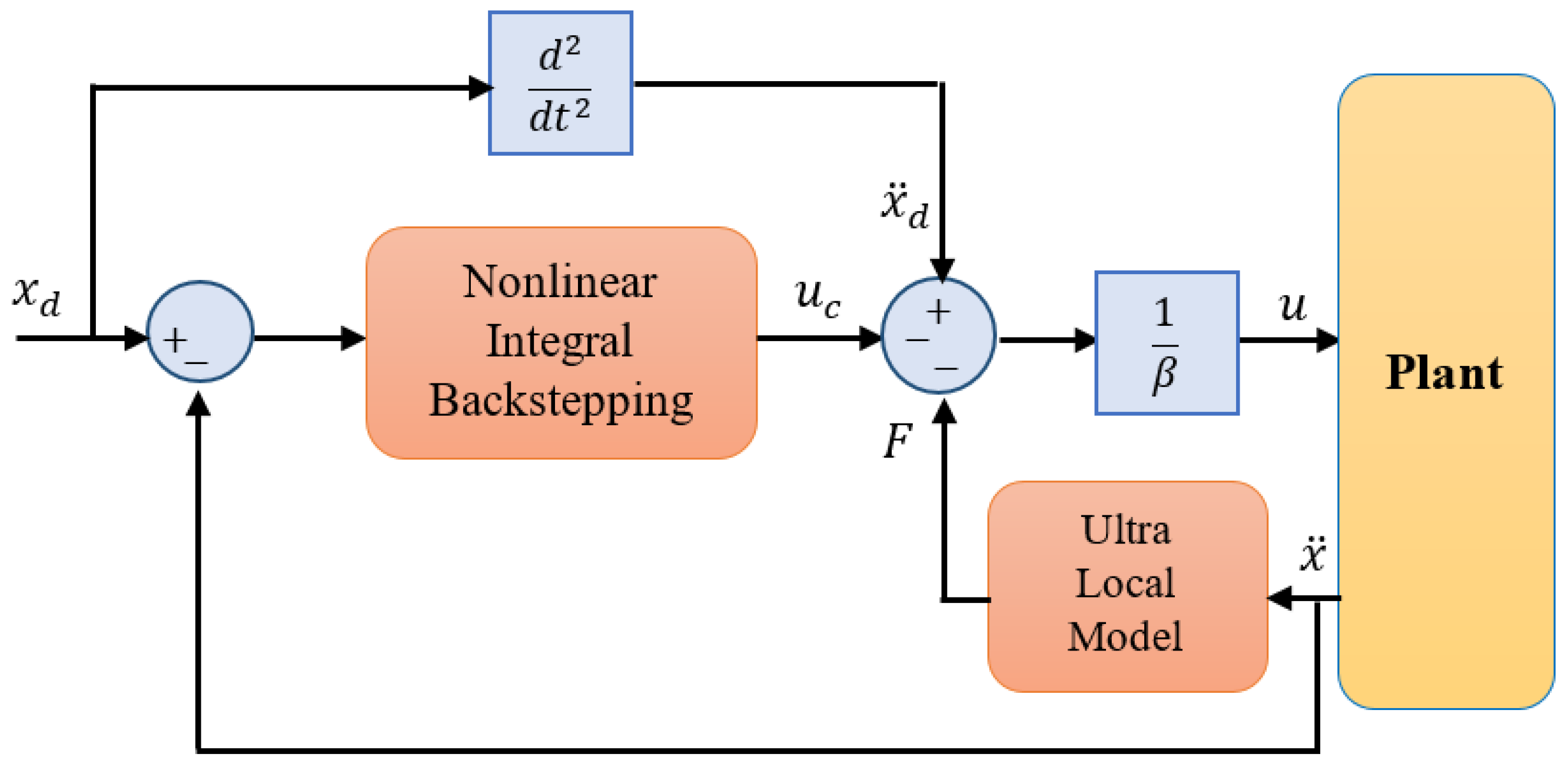
The position tracking and velocity tracking error can be convergence to a certain variable by using the theory of NIB-MFC. The block diagram of this control loop has been illustrated in Figure 2 [30,31].
The Lyapunov function is chosen to guarantee the convergence stability of the nonlinear WT system for this purpose. The Lyapunov function V ( e 1 ) will be defined to be positive definite around the state variable and can be written as:
V 1 ( e 1 ) = 1 2 e 1 2
The derivative of this function is shown as follows:
V ˙ 1 ( e 1 ) = e 1 e ˙ 1 = e 1 ( x 2 x ˙ d )
Since, x 2 is not our control input, there will be a dynamic error between it and its desired value, x 2 d . Therefore, the velocity tracking error can be offered to compensate for the dynamics error:
e 2 = x 2 x 2 d
The error will go to zero if the Lyapunov function is chosen semi-negative. The implicit input x 2 can be written as:
x 2 d = x ˙ d k 1 e 1
e 2 = x 2 x ˙ d + k 1 e 1
The modeling error and uncertainties lead to steady-state error. This error can be eliminated by using the integral term to the system as shown in below:
x 2 = x ˙ d k 1 e 1 k 3 e 1
e 2 = x 2 x ˙ d + k 1 e 1 + k 3 e 1
As a result, the derivative of velocity and position tracking can be described as:
e ˙ 1 = x ˙ 1 x ˙ d = e 2 + x * x ˙ d = e 2 k 1 e 1 k 3 e 1
e ˙ 2 = x ˙ 2 x ¨ d + k 1 e ˙ 1 k 3 e 1 = x ˙ 2 x ¨ d + k 1 e 2 k 1 2 e 1 k 1 k 3 e 1 k 3 e 1
The Lyapunov function V 1 ( e 1 . e 1 ) and V 2 ( e 1 . e 2 . e 1 ) will be defined for the position and velocity tracking error and formulated as [31]:
V 1 ( e 1 . e 1 ) = 1 2 e 1 2 + k 3 2 ( e 1 ) 2
V ˙ 1 ( e 1 . e 1 ) = e 1 e ˙ 1 + k 3 e 1 e 1 = e 1 e 2 k 1 e 1 2
V 2 ( e 1 . e 2 .   e 1 ) = 1 2 e 1 2 + 1 2 e 2 2 + k 3 2 ( e 1 ) 2
V ˙ 2 ( e 1 . e 2 . e 1 ) = e 1 e ˙ 1 + e 2 e ˙ 2 + k 3 e 1 e 1 = e 1 e 2 k 1 e 1 2 + e 2 ( x ˙ 2 x ¨ d + k 1 e 2 k 1 2 e 1 k 1 k 3 e 1 k 3 e 1 )
To guarantee the convergence of the e 2 to zero the V ˙ 2 ( e 1 . e 2 . e 1 ) should be semi-negative definite. This can be satisfied by choosing the Equation (30).
e 1 e 2 + e 2 ( x ˙ 2 x ¨ d + k 1 e 2 k 1 2 e 1 k 1 k 3 e 1 k 3 e 1 ) = k 2 e 2 2
Consequently, x ˙ 2 can be written as:
x ˙ 2 = f ( x ) + x ¨ d + u c = x ¨ d + ( k 1 2 + k 3 1 ) e 1 ( k 1 + k 2 ) e 2 + k 1 k 3 e 1
u c = [ ( k 1 2 + k 3 1 )   e 1 ( k 1 + k 2 ) e 2 + k 1 k 3 e 1 ] f ( x )

3.2. Reinforcement Learning

Reinforcement learning (RL), due to its generality, is studied in many areas such as control theory, operations research, simulation-based optimization, multi-agent systems, statistics, and genetic algorithms [32]. The problems of interest in RL have also been studied in the theory of optimal control, which is concerned mostly with the existence and characterization of optimal solutions, particularly in the absence of a mathematical model of the environment. Therefore, in wind turbine plant, where the system is nonlinear and has huge complexities, RL is a powerful and practical tool to estimate controller parameters which control wind turbine blade pitch angle and consequently rotor speed under the various level of wind speed variations.
RL is employed by various software and machines to find the best possible behavior or path it should take in a specific situation. But to implement RL operationally which are mainly continuous control problems, there are many problems including the divergence of learning, continuous nature of inputs and outputs and temporal correlation of data.
Recently, deep Q-network (DQN) has introduced a new set of features to solve most of the problems mentioned. However, a number of these challenges such as continuous states which are especially related to practical applications, cannot be resolved by this algorithm. In this regard, deep deterministic policy gradients (DDPG) had been proposed by Lillicrap et al. [33] based on the significant progress in DQN and the new approach named actor-critic paradigm expressed in [34] as a method which tackles continuous control issues.

3.3. The Learning Process

Firstly, the following concepts which are related to RL are explained below:
  • Markov decision process (MDP): It is the form in which the RL environment is typically stated, and it is because many RL algorithms for this context utilize dynamic programming techniques.
  • Agent: The agent receives rewards by performing correctly and penalties for performing incorrectly. The agent learns without intervention from a human, by maximizing its reward and minimizing its penalty.
  • Environment: The environment is the physical world in which the agent operates. The agent’s current state and action are considered as its input, and the agent’s reward and its next state are its output.
  • State: State s is the current situation of the agent in the environment, and S is the set of all possible states of the agent.
  • Policy: Policy π is the method by which the agent’s state is mapped to an appropriate action leading to the highest reward.
  • Action: A is the set of all possible moves a , that the agent can make.
  • Reward: This value is the feedback from the environment as an evaluation criterion that determines the success or failure of an agent’s actions in a given state.
  • Value function: The value function V π is defined as the long term expected to return with a discount. The discount factor ( γ   ϵ   ( 0 , 1 ] ) dampens the rewards’ effect on the agent’s choice of action to make future rewards worth less than immediate rewards. Roughly speaking, the value function estimates “how good” it is to be in a given state.
  • Q-value: Q-value or action value is used to measure how effective taking an action at a state is.
From the practical point of view, the interaction between an active decision-making agent and its environment happens in all RL applications. On the other words, the agent tries to achieve a goal, through maximizing reward, despite uncertainty about its environment.
The standard reinforcement learning theory expresses that an agent obtains a policy, which maps every state s   ϵ   S to an action a   ϵ   A . It maximizes the expectation of a long-term discounted reward as below:
J = E r i . s i ~ E . a i ~   π [ R 1 ]
where R t = k = 0 γ k r t + k is the total long term discounted reward at each step.
A value function V π which is formulated in Equation (34), depicts the total discounted reward R t for each s   ϵ   S .
V π ( s ) = E π [ R t | s t = s ]
The value function,   V π can be recursively described as Equation (35) according to the Bellman Equation:
V π ( s ) = E π [ r t + γ V π ( s t + 1 ) | s t = s ]
An equivalent of the value function is represented by the action-value function Q   π in Equation (36), given as [35]:
Q   π ( s .   a ) = E π [ r t + γ Q π ( s t + 1 . a t + 1 ) | s t = s . a t = a ]
The policy shall be chosen in such a way that it maximizes the action-value function. On the other hand, π * = arg max a Q * ( s . a ) .
The DDPG algorithm having a great ability to solve continuous problems consists of two neural networks (NNs)   μ ( s t | θ μ ) and Q ( s t . a t | θ Q ) named actor NN (ANN) and critic network (CNN), where θ Q and θ μ are the weights of the CNN and ANN, respectively. According to the stochastic gradient descent, the CNN is updated by minimizing the loss function below [36,37]:
( θ Q ) = E ( s . a ) [ ( y t Q ( s t .   a t | θ Q ) ) 2 ]
where
y t = r t ( s t .   a t ) + γ Q ( s t + 1 . μ ( s t | θ μ )   | θ Q )
Based on the policy of Equation (39), the coefficients of ANN are updated.
θ μ J θ μ E s t ~ ρ β [ θ μ Q ( s . a | θ Q ) | a = μ ( s | θ μ ) θ μ μ ( s | θ μ ) ] = E s t ~ ρ β [ a Q ( s . a | θ Q ) | a = μ θ ( s ) θ μ μ ( s | θ μ ) ]
In the above equation,   β is a specific policy to the current policy   π and ρ is the discounted distribution.
Due to correlations existing in the input experiences, a replay buffer D is used to weaken that in the DDGP algorithm. To enable a robust learning DDPG agent, two separate NNs μ ( s | θ μ ) and Q ( s . a | θ Q ) named target NNs (TNNs) are utilized in addition to the main ANN and CNN. The additional NNS are same in shape to the main NNs but have distinct coefficient weights θ [38,39,40].

4. Digital Twin Controller of WT System

4.1. The Concept of Digital Twin

Nowadays, modeling and simulation is a standard process in system development. The digital twin (DT) concept refers to the accurate reproduction of a physical wind turbine in a computational system to facilitate understanding and study its behavior [41,42]. This digital twin can empower wind asset owners and turbine manufacturers operating wind turbines to predict and plan for faults and optimize the performance of their assets. The technology involves creating a digital copy or “twin” of physical assets, processes, systems, and devices to allow real-time remote monitoring that can save the wind industry significant downtime and maintenance costs while increasing production. Real-time data from sensors is fed into the digital twin and compared to simulated theoretical parameters under the same working conditions. Then similarities and discrepancies are analyzed to diagnose the health of the asset.
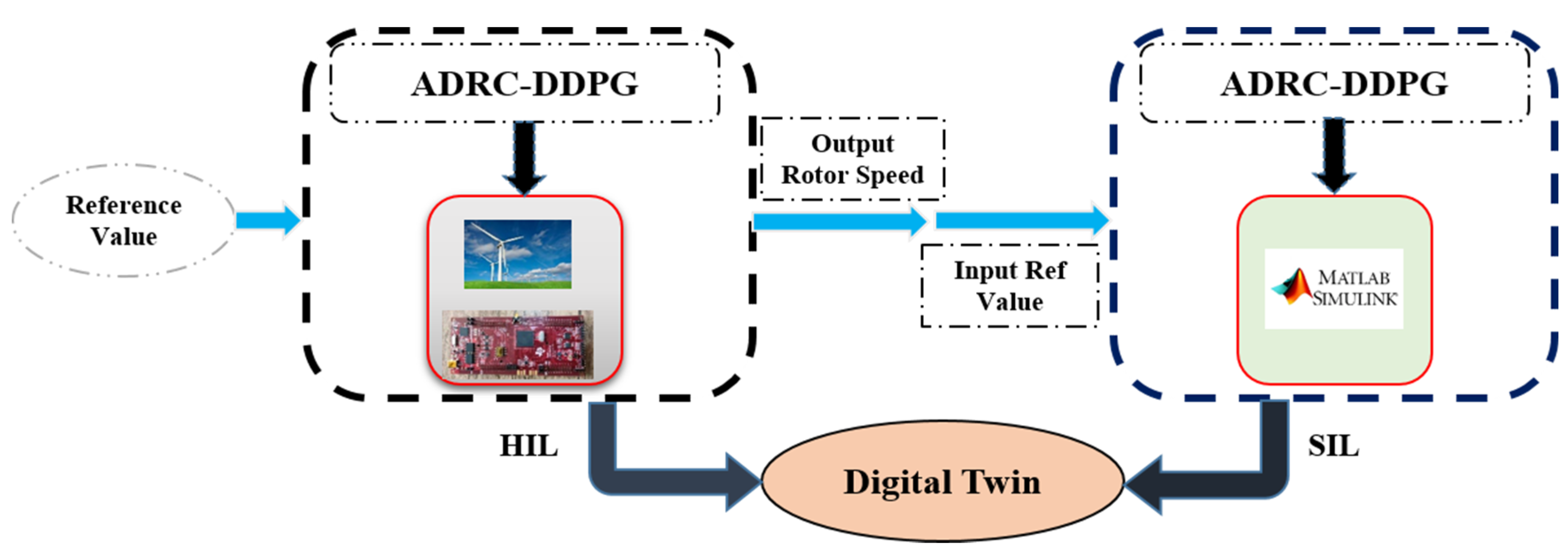
In this paper, to achieve the mentioned purposes, it has been illustrated how a digital twin of the pitch angle controller implements on a TMS320F28379D Dual-Core Delfino™ Microcontroller device in Texas Instrument (TI). The hardware-in-loop (HIL) idea develops a controller algorithm to diagnose the health of its behavior on the wind turbine. However, the software-in-the-loop (SIL) idea permits the test of the algorithms but neglects the test of the controller hardware. In this paper, it provides some strategies for HIL and SIL model with DT concept that it is outlined in the list below:
  • Define the system and simulation of closed-loop control in software;
  • Implementation of the proposed controller on a TI microcontroller board;
  • Upgrade the controller coefficients and achieving the desired output using the DDPG-NIB method in HIL mode with real-time data;
  • Optimization of control coefficients of SIL controller reusing NIB-DDPG method (criteria: similarity of SIL and HIL outputs).
It would appear logical to conclude that these strategies refer to the outputs and performances of the two systems are similar. It is possible to estimate the behavior of the system in HIL mode by changing its parameters in SIL mode. At the first step, the NIB-MFC of the HIL setup is regulated to reduce the rotor speed deviations in the WT system. Following this, the NIB-MFC of SIL is designed in such a way that it minimizes the difference between the outcome of the WT in the HIL and SIL environments. Thus, the design of the DT controller for the WT plant is carried out in two distinct steps which are illustrated in Figure 3.

4.2. The Proposed DDPG Tuned Backstepping Control Method

The parameter estimation accuracy of the backstepping controller highly affects the quality of its output actions. Therefore, the proposed DDPG algorithm is used to design the coefficients embedded in the NBI controller structure to offers a new as an adaptive tuner mechanism (instead of tuning manually). In the backstepping controller, the NIB block has a nonlinear attitude, especially in temporary variable variations which leads to controller performance deterioration. Thus, the best solution to tackle this issue is to adaptively calculate the NIB gains ( k 1 , k 2 and k 3 ) based on the DDPG algorithm. The structure of the proposed DDPG backstepping method leading to have a constant output rotor angular velocity is represented in Figure 4. In this structure, the DDPG algorithm provides tuner signals to adjust the NIB-MFC gains adaptively.
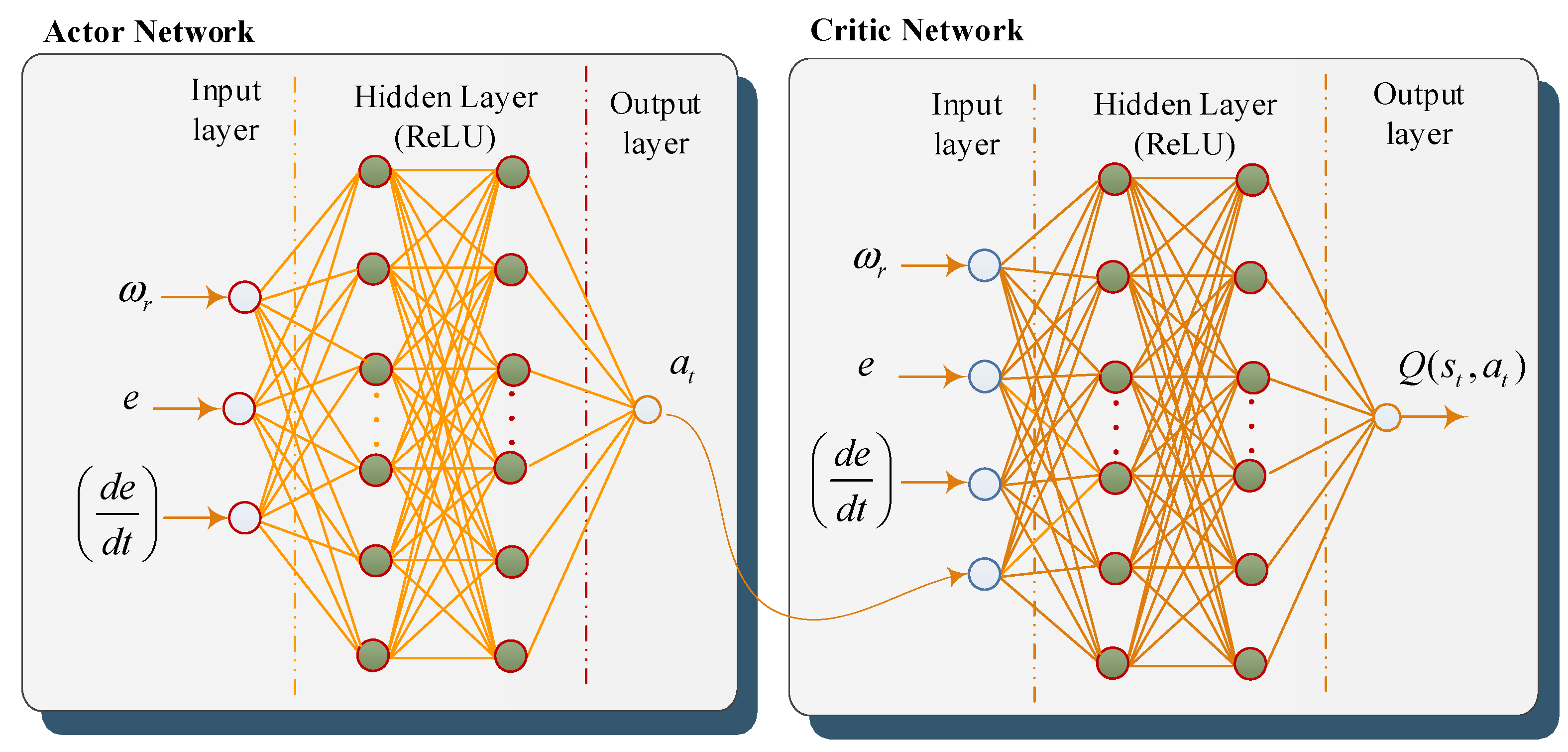
The critic network in the proposed structure is responsible for the effectiveness evaluation of the actor policy, and according to the critic network data, the ANN adjusts the NIB gains to reach the controller objective. The ANN senses the state variables and then generates three continuous control signals for tuning of the NIB gains ( k 1 ,   k 2 and k 3 ). After that, the CNN receives the state variables and turning signals, and then reward signal r t is calculated. Following that, the critic network weights are trained to lead to an updated DDPG network with adaptive tuning action signals to feed the controller.
The terms of rotor speed, rotor speed error, and rotor speed error integral as are chosen here in both the HIL and SIL to form a three-dimensional vector of state space, represented as:
s t = { ω r , e , e d t }
where s t is the state of the MDP in the HIL and SIL environments.
In this application, the structure of the NNs of the DDPG algorithm for the design of the HIL and SIL controllers is the same with two hidden layers of 200 and 100 units. The architecture of the ANN and CNN for online tuning of the HIL and SIL controllers are illustrated in Figure 5, where the rectified linear unit (ReLU) is chosen as the activation function. As depicted in Figure 5, the inputs of the ANN are the system states while the ANN output and system states are inserted into the CNN.
To determine the optimal control coefficients based on the DT concept, the reward function of the DDPG algorithm for the design of HIL and SIL controllers is defined as Equations (41) and (42), respectively.
r e w a r d   i n   H I L = 1 ( r o t o r   s p e e d   e r r o r ) 2
r e w a r d   i n   S I L = 1 | d i f f e r e n c e   b e t w e e n   t h e   r o t o r   s p e e d   o f   H I L   a n d   S I L |

4.3. Implementing the Adaptive NIB Controller Based DDPG

The training procedure of the DDPG mechanism for online tuning of the NBI controller coefficients in the HIL and SIL environments are the same which is described in the following manner.
The ANN and CNN μ ( s t | θ μ ) and Q ( s t ,   a t | θ Q ) , with coefficient weights θ μ and θ Q , respectively, are initialized randomly. The TNNs θ Q and θ μ are updated with weights of θ Q θ Q and θ μ θ μ , respectively. A replay buffer with the capacity D is constructed. The initial state is s 1 stored. The action a t = [ k 1 ,   k 2 , k 3 ] = μ ( s t | θ μ ) + nosie is chosen based on ANN. The action a t is applied to the system (HIL or SIL controllers) to obtain the next state s t + 1 and reward r t —the reward is calculated by Equations (41) and (42) for HIL and SIL, respectively. The term ( s t , a t , r t ,   s t + 1 ), which is the experience set at each time step, is saved in the R -sized experience memory. During each step of the training process, a mini-batch of experiences saved previously are uniformly sampled from the memory D to update the NNs at each time step. y t = r t ( s t .   a t ) + γ Q ( s t , μ ( s t | θ μ )   | θ Q ) is calculated, the CNN is updated by minimizing the loss ( θ Q ) = E ( s . a ) [ ( y t Q ( s t ,   a t | θ Q ) ) 2 ] . The policy of ANN is updated by using the following policy gradient: θ μ J θ μ = E s t ~ ρ β [ a Q ( s t ,   a t | θ Q ) | a = μ θ ( s ) θ μ μ ( s t | θ μ ) ] . The TNN’s are updated by the following learning mechanism:
θ Q τ θ Q + ( 1 τ ) θ Q   and   θ μ τ θ μ + ( 1 τ ) θ μ
where τ 1 .

5. Results

The NIB-MFC scheme, which is a model-free scheme with an ultra-local model, offers optimal performance to compensate system output of the WT plant in the digital twin framework. For this purpose, the NBI-MFC controller has been adopted in the HIL and SIL environments. The gains of the NIB-MFC technique, which play a critical role in the pitch angle control of a WT plant, are considered as the control coefficients which should be adjusted by the DDGP tuner mechanism. The DDPG method throughout 200 episodes, which is equal to 2500 training steps.
It can be said that the target of using digital twin is the similarity system’s output behaviors in the SIL and HIL. If this purpose is satisfied, then it is possible to estimate the behavior of the HIL system by changing the parameters in the SIL system. To achieve similarity behaviors of system output in the digital twin system, firstly deep deterministic policy gradient (DDPG) based nonlinear integral backstepping (NIB) in combination with model free control (MFC), (DDPG-NIB-MFC), is used to obtain optimal controller parameters by reducing differences between reference input and output in HIL and after that, HIL pitch angle output is applied as reference input in SIL. In the subsequent section, the performance of the suggested control system is performed by real-time software-in-the-loop (RT-SIL) MATLAB simulation experiments, as well as real-time hardware-in-the-loop (RT-HIL) TI board. Moreover, the backstepping and proportional-integral (PI) controllers are also designed by the particle swarm optimization (PSO) algorithm in the digital twin framework for the comparative purposes. By minimizing the objective function, the controller coefficients are optimally designed. In this application, the inverse values of the reward functions for the HIL and SIL controllers (defined in Equations (41) and (42)) were defined as objective functions.

5.1. Scenario I

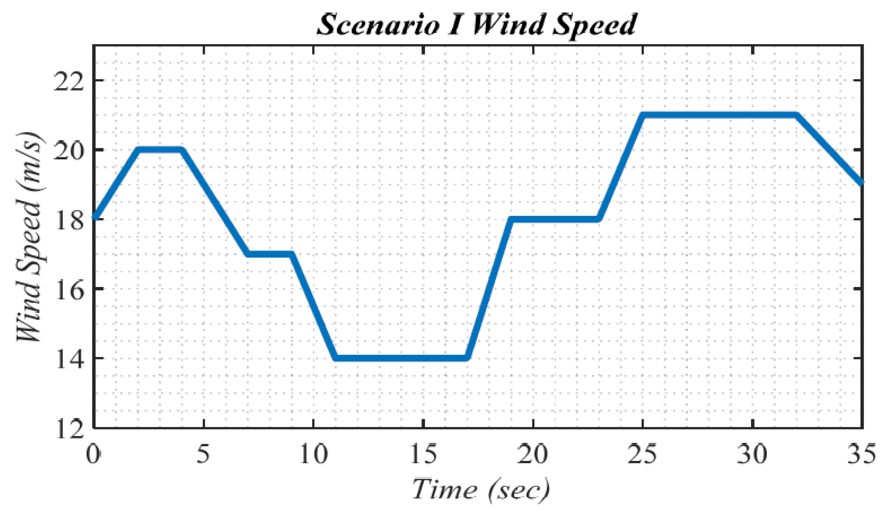
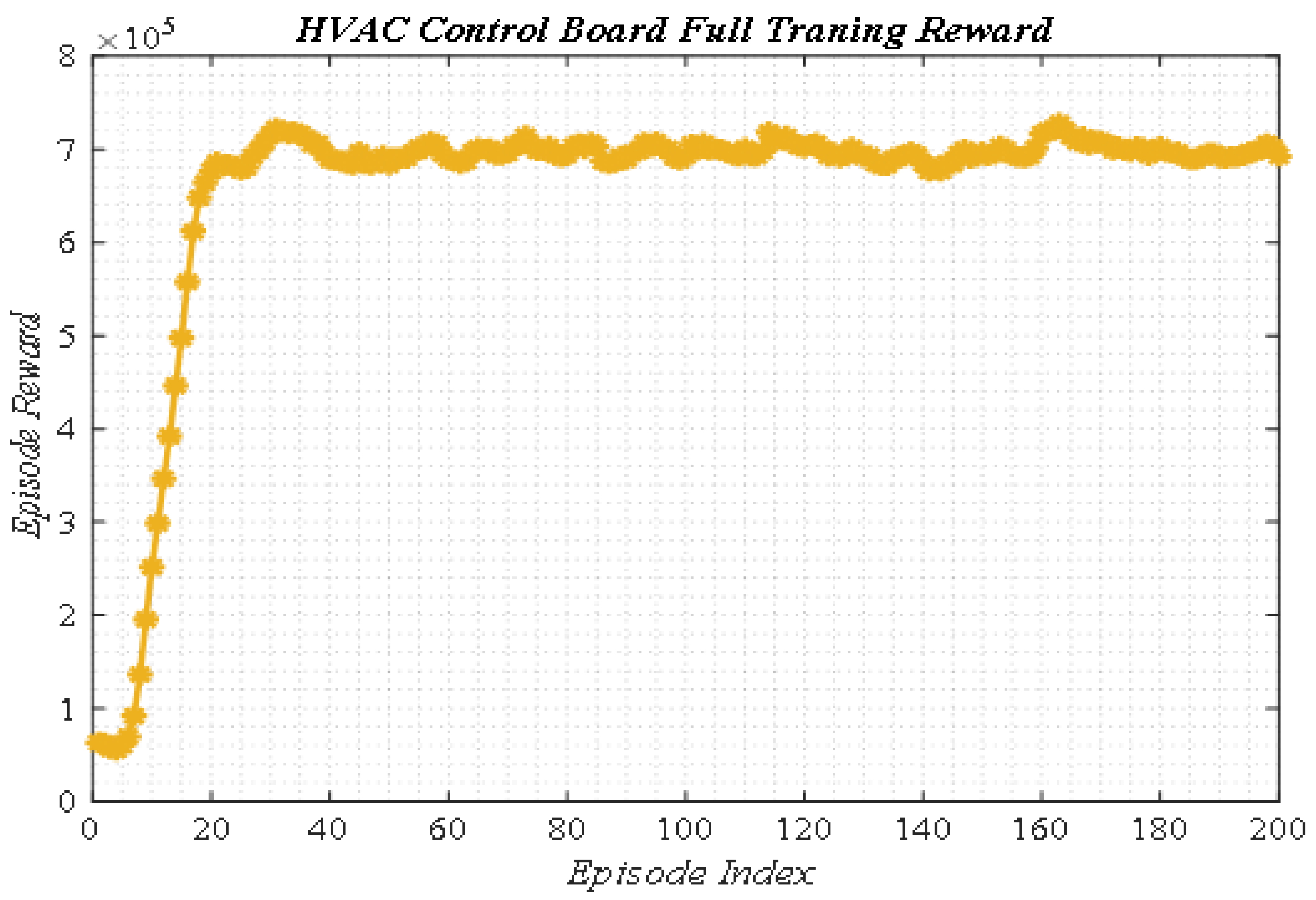
At the first stage, a multi-step wind speed variation in the range of [14 m/s, 21 m/s] is applied to the non-linear WT system. The profile of the wind speed disturbance is depicted in Figure 6 while the rotor speed curves of the HIL system for the backstepping based DDPG, PSO optimized backstepping and PI controllers are shown in Figure 7. From the comparative outcomes of Figure 7, the suggested backstepping controller based DDPG offers a superior dynamic performance having a lesser settling time and smaller amplitude of fluctuations than the backstepping controller based PSO in the terms. It is also seen that the outcome of the PI controller based PSO experiences large-angle rotor speed fluctuation and thus it cannot compensate for the multi-step wind speed variation. The curve of the average reward for the full-simulated training phase under the wind disturbance is depicted in Figure 8. Looking at the details, as it regards Figure 8, the reward started at 200,000, then the value goes up significantly since episode 5, at which point it almost constant. The increasing trend of the reward measured in HIL is an indicator of the reduction of rotor speed error which confirms the correctness of the suggested NBI controller designed by the DDPG algorithm.
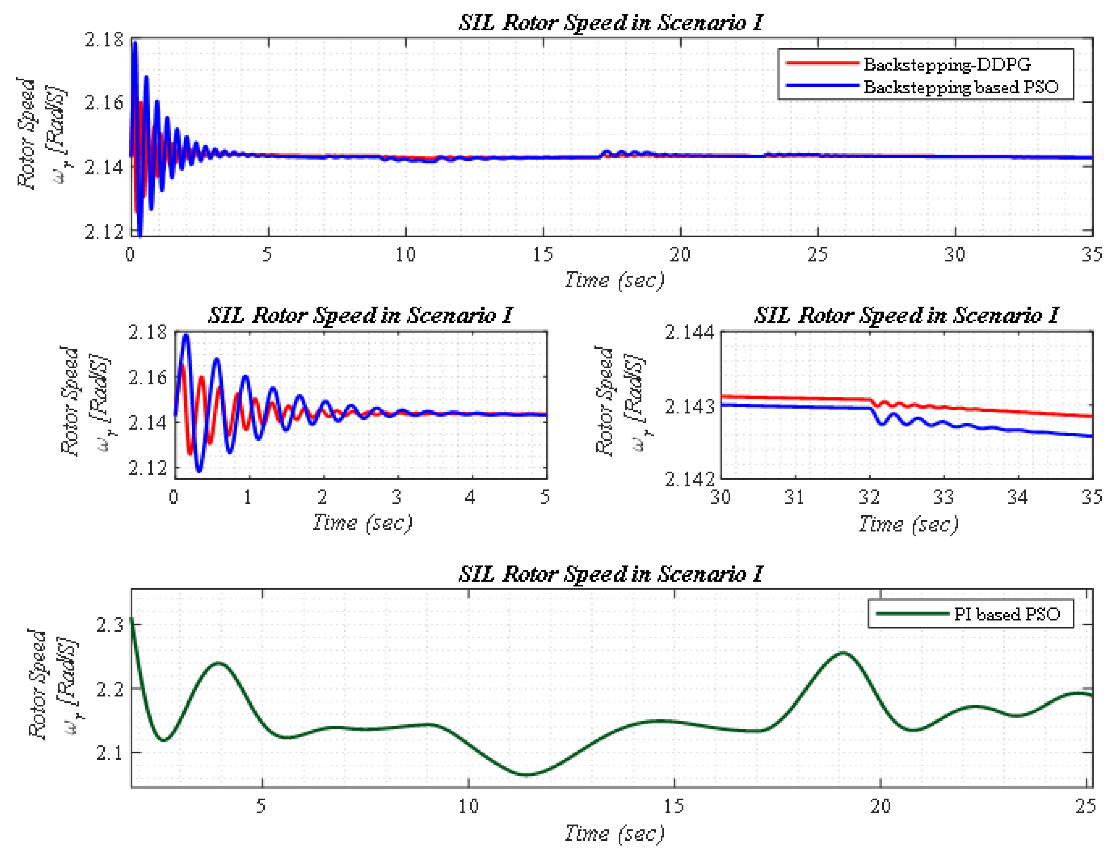
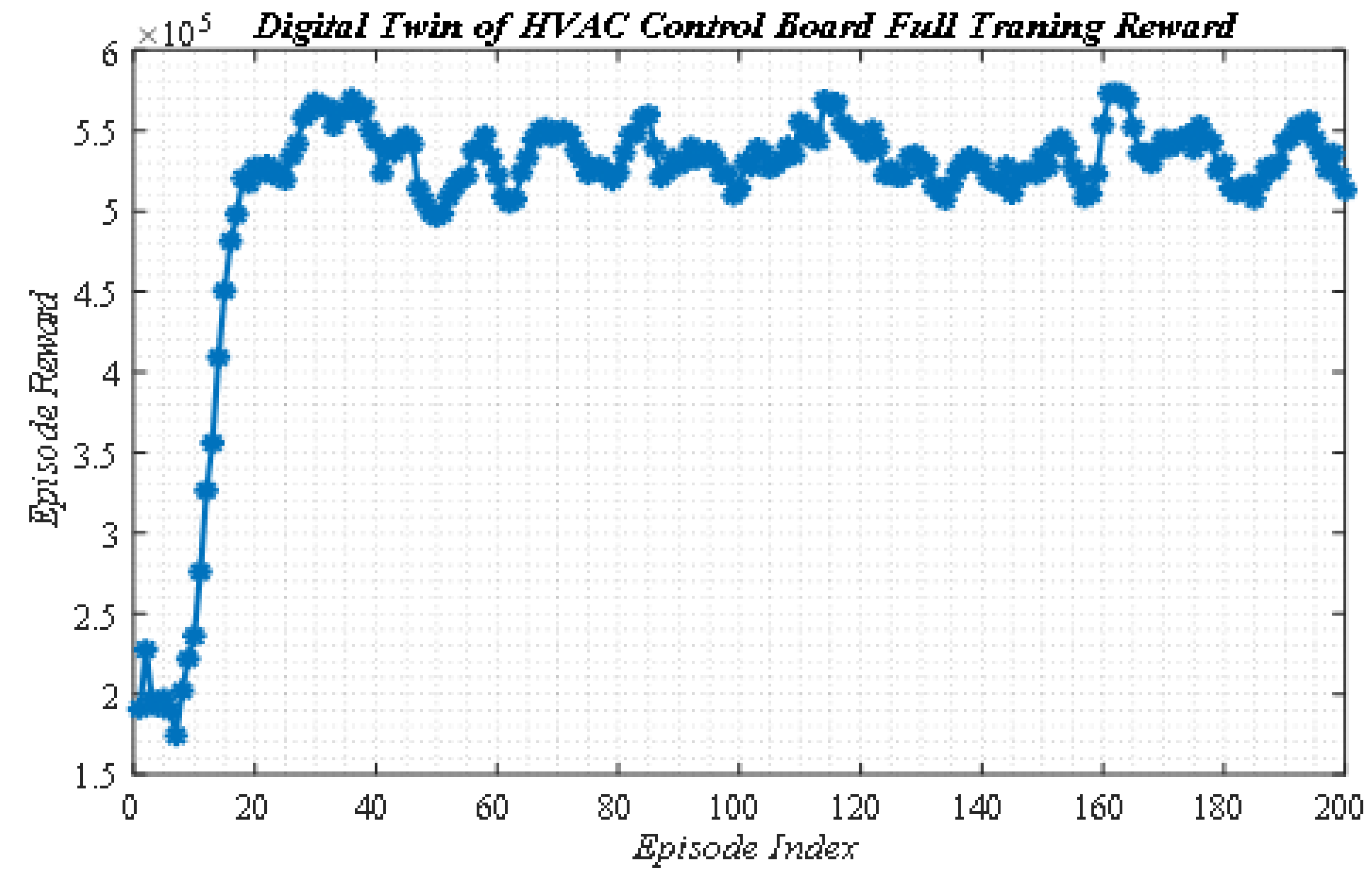
Similarly, the rotor speed outcomes of the SIL for the backstepping based DDPG, PSO optimized backstepping and PI controllers are compared as illustrated in Figure 9. Critical observation of the SIL outcomes reveals that the suggested controller gives a higher quality transient and steady-state behavior of rotor speed compared to the PSO optimized backstepping and PI controllers. Figure 10 depicts that the DDPG agent is trained over 200 episodes to adaptively tune the backstepping controller coefficients. From Figure 10, it is clear that the average reward is increased and stabled during the 200 episodes which means the difference between the system outcomes in HIL and SIL is minimized. This affirms the efficiency of the DDPG agent in tuning the backstepping controller in the digital twin concept.
The dynamic specifications of the WT system with the multi-step wind speed in the terms of settling time, overshoot and error output are noted and furnished in Table 1. For comparison, the obtained outcomes reached for both HIL and SIL environments are provided in Table 1. From the statistical analysis, by employing the backstepping controller based DDPG, an improvement in the dynamic specifications of digital twin-based system is achieved for both the HIL and SIL.

5.2. Scenario II

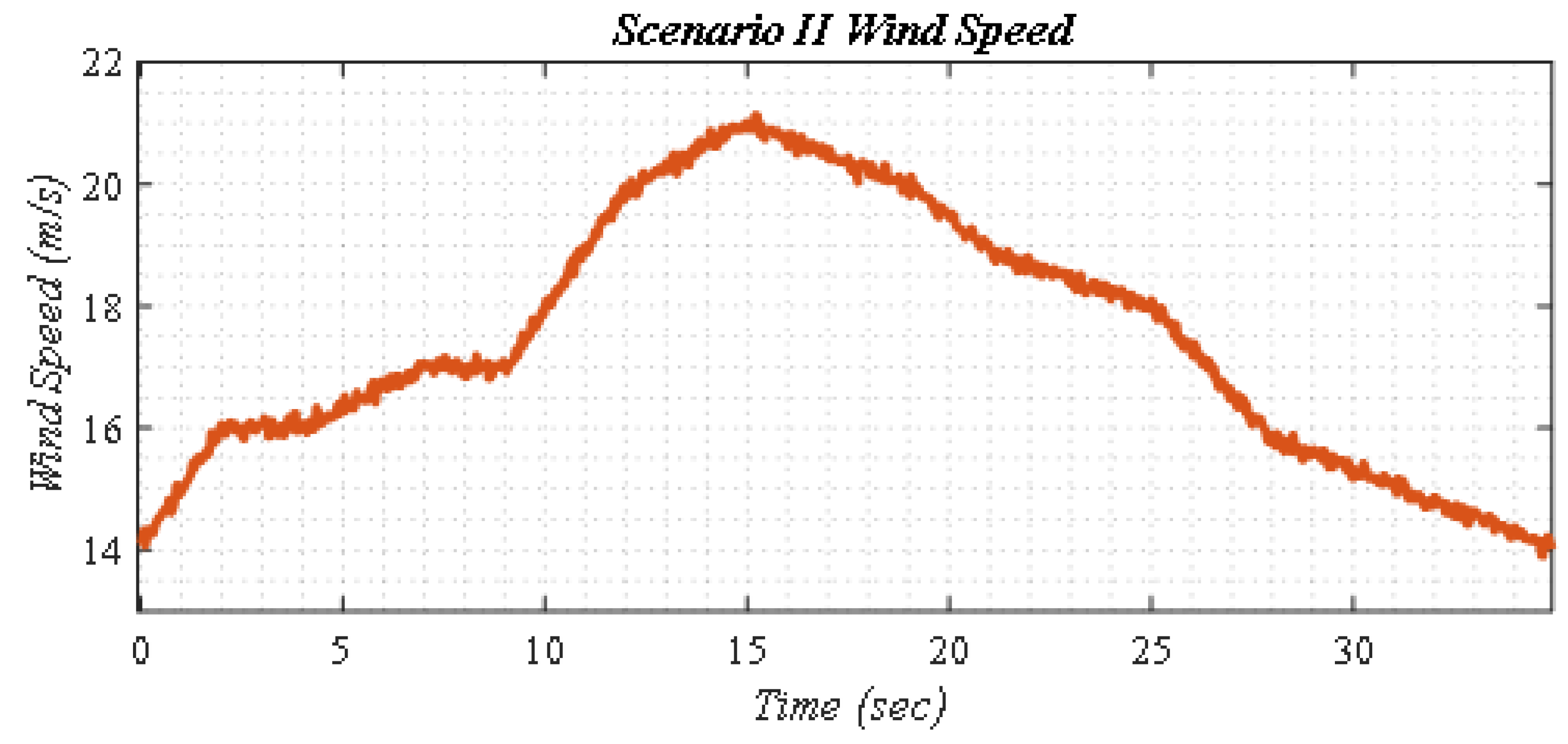
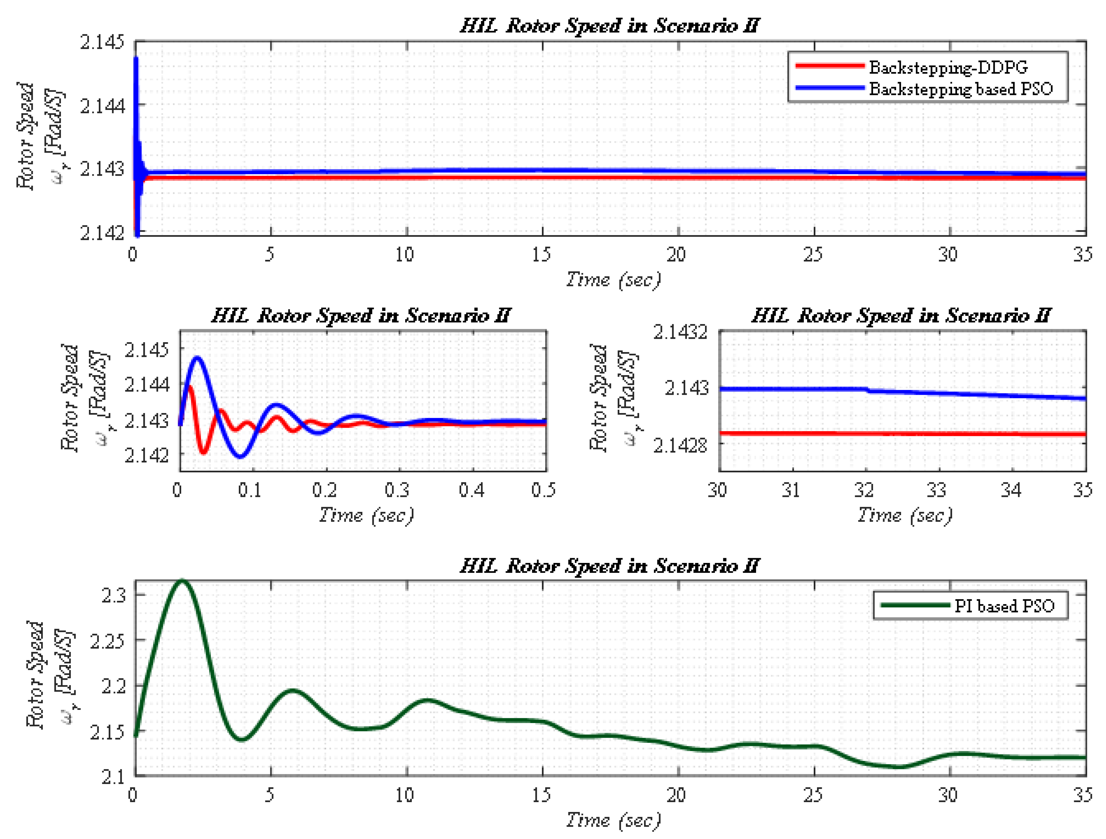
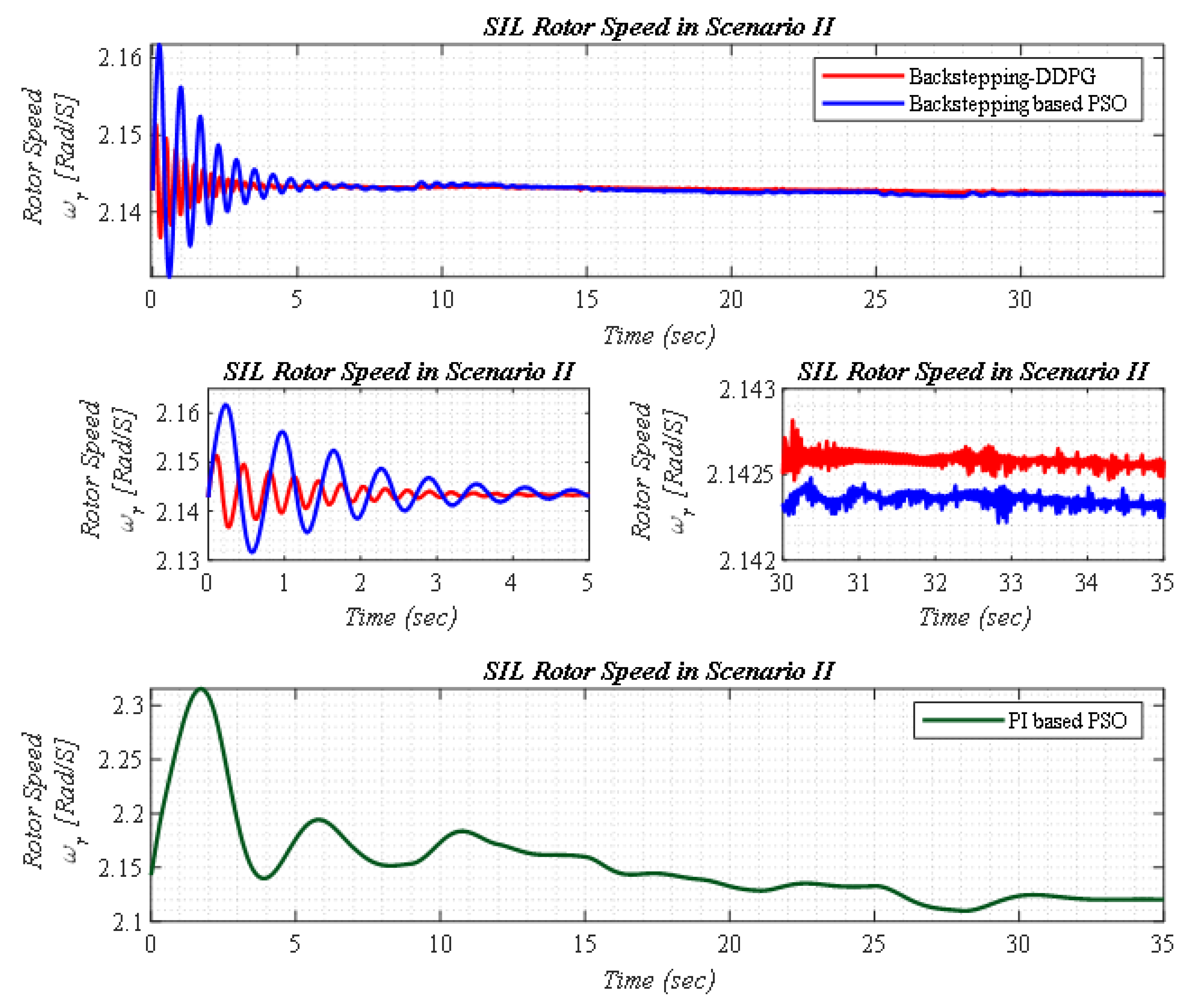
In this case, the applicability of the suggested digital twin controller is explored when the wind speed is randomly fluctuated within [14 m/s, 22 m/s]. The profile of the random wind speed (which is numerically produced by an additive Gaussian noise with noise power 0.0003 to DC and slope levels at different time intervals) is presented in Figure 11 and the comparative dynamic outcomes for the HIL and SIL controllers are illustrated in Figure 12 and Figure 13, respectively. The outcomes of these figures prove the superiority of the backstepping controller based DDPG to damp the rotor speed in the HIL environment. In addition, it is demonstrated that the curves of rotor speed are very close to each other in both HIL and SIL dynamic outcomes.

5.3. Scenario III (The Parametric Uncertainty in the Turbine Model)

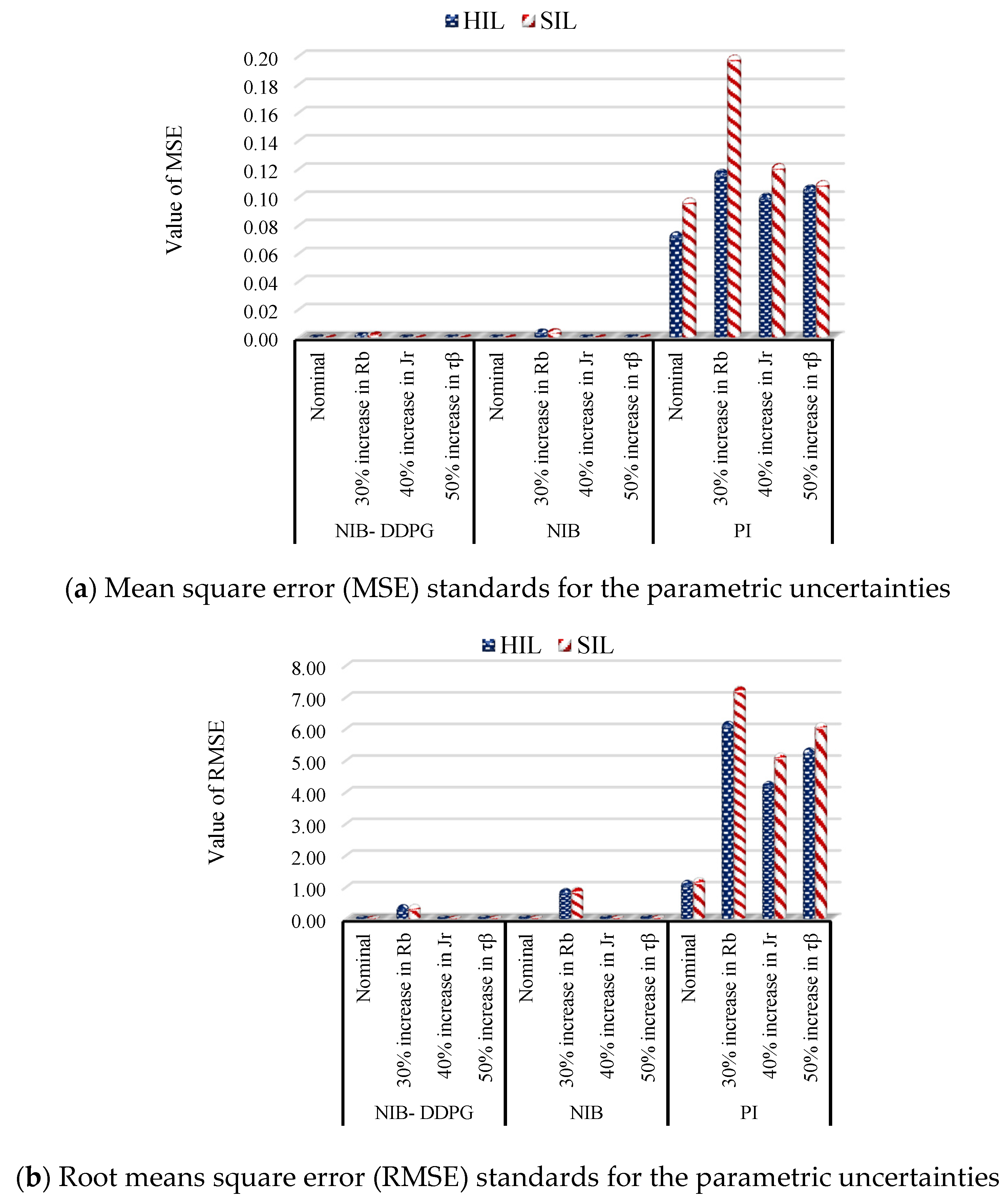
For an illustration of the robustness ability of suggested backstepping controller based DDPG, some uncertainties are imposed on the WT model parameters under the following: RB = +30%, JR = +40% and TB = +50%. Two standard error measurement criteria including the mean square error (MSE) and the root mean square error (RMSE) are considered, which are defined as:
M S E = 1 n i = 1 n [ e i 2 ]
R M S E = 1 n i = 1 n [ e i 2 ]
The MSE and RMSE values for the HIL and SIL are provided in Figure 14a,b, respectively. From the bar comparison graphs, it is proved that the backstepping controller based DDPG has less sensitivity than other controllers to increasing of rotor radius, rotor inertia and pitch actuator time constant. It is also confirmed that by employing the suggested controller, the behavior of SIL output is the same as HIL output variations and this means that the concept of the digital twin is fulfilled.

6. Conclusions

This paper focuses on presenting a novel backstepping controller based DDPG for a pitch angle control of variable speed WT in the digital twin framework. Initially, the backstepping controller based DDPG is adopted for control of WT in HIL to damp the rotor speed fluctuations in this environment. Following this, the digital twin of the WT system is constructed in SIL and DDPG algorithm is employed to tune the NIB controller coefficients by the measured data from the WT in the HIL environment. The digital twin realization of the suggested scheme has been implemented on a TMS320F28379D dual-core Delfino™ microcontroller device in Texas Instrument (TI). The results revealed that the dynamic responses of the WT speed rotor are improved with the backstepping controller based DDPG. Moreover, the suggested control scheme can tune the SIL controller coefficients and make the digital twin WT system has the same operation with the HIL. From the analysis, it is found that the presented controller is more efficient and reliable than the PSO optimized backstepping and classical PI controllers.

Author Contributions

Data curation, S.A. and M.J.Z.; Methodology, A.P.; Software, S.-R.M.; Supervision, M.-H.K.; Validation, M.G. All authors have read and agreed to the published version of the manuscript.

Funding

This research received no external funding.

Conflicts of Interest

The authors declare no conflict of interest.

References

  1. Rezaei, V. Advanced control of wind turbines: Brief survey, categorization, and challenges. In Proceedings of the 2015 American Control Conference (ACC), IEEE, Chicago, IL, USA, 1–3 July 2015; pp. 3044–3051. [Google Scholar]
  2. Chen, J.; Chen, J.; Gong, C. New Overall Power Control Strategy for Variable-Speed Fixed-Pitch Wind Turbines within the Whole Wind Velocity Range. IEEE Trans. Ind. Electron. 2012, 60, 2652–2660. [Google Scholar] [CrossRef]
  3. Boukhezzar, B.; Siguerdidjane, H. Nonlinear Control of a Variable-Speed Wind Turbine Using a Two-Mass Model. IEEE Trans. Energy Convers. 2010, 26, 149–162. [Google Scholar] [CrossRef]
  4. Leithead, W.E.; De La Salle, S.A.; Reardon, D. Classical control of active pitch regulation of constant speed horizontal axis wind turbines. Int. J. Control. 1992, 55, 845–876. [Google Scholar] [CrossRef]
  5. Wright, A.D. Modern Control Design for Flexible Wind Turbines; National Renewable Energy Laboratory: Golden, CO, USA, 2004. [Google Scholar]
  6. Lather, J.; Dhillon, S.; Marwaha, S. Modern control aspects in doubly fed induction generator based power systems: A review. Int. J. Adv. Res. Electr. Electr. Instrum. Eng. 2013, 2, 2149–2161. [Google Scholar]
  7. Trabelsi, R.; Khedher, A.; Mimouni, M.F.; M’Sahli, F. An Adaptive Backstepping Observer for on-line rotor resistance adaptation. Int. J. IJ-STA 2010, 4, 1246–1267. [Google Scholar]
  8. Ullah, N.; Wang, S. High performance direct torque control of electrical aerodynamics load simulator using adaptive fuzzy backstepping control. Proc. Inst. Mech. Eng. Part G J. Aerosp. Eng. 2014, 229, 369–383. [Google Scholar] [CrossRef]
  9. Rajendran, S.; Jena, D. Backstepping sliding mode control of a variable speed wind turbine for power optimization. J. Mod. Power Syst. Clean Energy 2015, 3, 402–410. [Google Scholar] [CrossRef] [Green Version]
  10. Fliess, M.; Join, C. Model-free control and intelligent pid controllers: Towards a possible trivialization of nonlinear control? IFAC Proc. Vol. 2009, 42, 1531–1550. [Google Scholar] [CrossRef] [Green Version]
  11. Fuglsang, P.; Madsen, H.A. Optimization method for wind turbine rotors. J. Wind. Eng. Ind. Aerodyn. 1999, 80, 191–206. [Google Scholar] [CrossRef]
  12. Selig, M.S.; Coverstone-Carroll, V.L. Application of a Genetic Algorithm to Wind Turbine Design. J. Energy Resour. Technol. 1996, 118, 22–28. [Google Scholar] [CrossRef] [Green Version]
  13. Wiering, M.; Van Hasselt, H. Ensemble Algorithms in Reinforcement Learning. IEEE Trans. Syst. Man Cybern. Part B (Cybern.) 2008, 38, 930–936. [Google Scholar] [CrossRef] [Green Version]
  14. Watkins, C.J.C.H. Learning from Delayed Rewards; King’s College: London, UK, 1989. [Google Scholar]
  15. Rummery, G.A.; Niranjan, M. On-Line Q-Learning Using Connectionist Systems; University of Cambridge, Department of Engineering Cambridge: Cambridge, UK, 1994. [Google Scholar]
  16. Sutton, R.S. Generalization in reinforcement learning: Successful examples using sparse coarse coding. In Advances in Neural Information Processing Systems; University of Massachusetts: Amherst, MA, USA, 1996; pp. 1038–1044. [Google Scholar]
  17. Sutton, R.; Barto, A. Reinforcement Learning: An Introduction. IEEE Trans. Neural Netw. 1998, 9, 1054. [Google Scholar] [CrossRef]
  18. Wiering, M.A.; Van Hasselt, H. Two Novel On-policy Reinforcement Learning Algorithms based on TD(λ)-methods. In Proceedings of the 2007 IEEE International Symposium on Approximate Dynamic Programming and Reinforcement Learning, Honolulu, HI, USA, 1–5 April 2007; pp. 280–287. [Google Scholar] [CrossRef]
  19. Sutton, R.S.; McAllester, D.A.; Singh, S.P.; Mansour, Y. Policy gradient methods for reinforcement learning with function approximation. In Advances in Neural Information Processing Systems; AT&T Labs-Research: Florham Park, NJ, USA, 2000; pp. 1057–1063. [Google Scholar]
  20. Baxter, J.; Bartlett, P. Infinite-Horizon Policy-Gradient Estimation. J. Artif. Intell. Res. 2001, 15, 319–350. [Google Scholar] [CrossRef]
  21. Moore, A.W.; Atkeson, C.G. Prioritized sweeping: Reinforcement learning with less data and less time. Mach. Learn. 1993, 13, 103–130. [Google Scholar] [CrossRef] [Green Version]
  22. Riedmiller, M. Neural Fitted Q Iteration—First Experiences with a Data Efficient Neural Reinforcement Learning Method. In European Conference on Machine Learning; Springer: Berlin/Heidelberg, Germany, 2005; Volume 3720, pp. 317–328. [Google Scholar]
  23. Pang, H.; Gao, W. Deep Deterministic Policy Gradient for Traffic Signal Control of Single Intersection. In Proceedings of the 2019 Chinese Control and Decision Conference (CCDC), Nanchang, China, 3–5 June 2019; pp. 5861–5866. [Google Scholar]
  24. Ghouri, U.H.; Zafar, M.U.; Bari, S.; Khan, H.; Khan, M. Attitude Control of Quad-copter using Deterministic Policy Gradient Algorithms (DPGA). In Proceedings of the 2019 2nd International Conference on Communication, Computing and Digital systems (C-CODE), Islamabad, Pakistan, 6–7 March 2019; pp. 149–153. [Google Scholar]
  25. Glaessgen, E.; Stargel, D. The Digital Twin Paradigm for Future NASA and U.S. Air Force Vehicles. In Proceedings of the 53rd AIAA/ASME/ASCE/AHS/ASC Structures, Structural Dynamics and Materials, Honolulu, HI, USA, 23–26 April 2012; p. 1818. [Google Scholar]
  26. Tao, F.; Sui, F.; Liu, A.; Qi, Q.; Zhang, M.; Song, B.; Guo, Z.; Lu, S.C.-Y.; Nee, A.Y.C. Digital twin-driven product design framework. Int. J. Prod. Res. 2018, 57, 3935–3953. [Google Scholar] [CrossRef] [Green Version]
  27. Rajendran, S.; Jena, D. Control of Variable Speed Variable Pitch Wind Turbine at Above and Below Rated Wind Speed. J. Wind. Energy 2014, 2014, 1–14. [Google Scholar] [CrossRef] [Green Version]
  28. Boukhezzar, B.; Siguerdidjane, H. Comparison between linear and nonlinear control strategies for variable speed wind turbines. Control Eng. Pr. 2010, 18, 1357–1368. [Google Scholar] [CrossRef]
  29. Ren, Y.; Li, L.; Brindley, J.; Shangguan, X.-C. Nonlinear PI control for variable pitch wind turbine. Control. Eng. Pr. 2016, 50, 84–94. [Google Scholar] [CrossRef] [Green Version]
  30. Al Younes, Y.; Drak, A.; Noura, H.; Rabhi, A.; El Hajjaji, A. Robust Model-Free Control Applied to a Quadrotor UAV. J. Intell. Robot. Syst. 2016, 84, 37–52. [Google Scholar] [CrossRef]
  31. Al Younes, Y.; Drak, A.; Noura, H.; Rabhi, A.; El Hajjaji, A. Nonlinear Integral Backstepping─Model-Free Control Applied to a Quadrotor System. In Proceedings of the 10th International Conference on Intelligent Unmanned Systems, Montreal, Canada, 29 September–1 October 2014. [Google Scholar]
  32. Wei, C.; Zhang, Z.; Qiao, W.; Qu, L. Reinforcement-Learning-Based Intelligent Maximum Power Point Tracking Control for Wind Energy Conversion Systems. IEEE Trans. Ind. Electron. 2015, 62, 6360–6370. [Google Scholar] [CrossRef]
  33. Gu, S.; Lillicrap, T.; Sutskever, I.; Levine, S. Continuous Deep Q-Learning with Model-based Acceleration. In Proceedings of the International Conference on Machine Learning, New York, NY, USA, 12–18 July 2016; pp. 2829–2838. [Google Scholar]
  34. Srinivasan, S.; Lanctot, M.; Zambaldi, V.; Perolat, J.; Tuyls, K.; Munos, R.; Bowling, M. Actor-Critic Policy Optimization in Partially Observable Multiagent Environments. In Advances in Neural Information Processing Systems; Advances in Neural Information Processing Systems: New York, NY, USA, 2018; pp. 3422–3435. [Google Scholar]
  35. Hasanvand, S.; Rafiei, M.; Gheisarnejad, M.; Khooban, M.-H. Reliable Power Scheduling of an Emission-Free Ship: Multi-Objective Deep Reinforcement Learning. IEEE Trans. Transp. Electrif. 2020, 1. [Google Scholar] [CrossRef]
  36. Gheisarnejad, M.; Khooban, M.H. An Intelligent Non-integer PID Controller-based Deep Reinforcement Learning: Implementation and Experimental Results. IEEE Trans. Ind. Electron. 2020, 1. [Google Scholar] [CrossRef]
  37. Hajihosseini, M.; Andalibi, M.; Gheisarnejad, M.; Farsizadeh, H.; Khooban, M.-H. DC/DC Power Converter Control-Based Deep Machine Learning Techniques: Real-Time Implementation. IEEE Trans. Power Electron. 2020, 1. [Google Scholar] [CrossRef]
  38. Khooban, M.H.; Gheisarnejad, M. A Novel Deep Reinforcement Learning Controller Based Type-II Fuzzy System: Frequency Regulation in Microgrids. IEEE Trans. Emerg. Top. Comput. Intell. 2020, 1–11. [Google Scholar] [CrossRef]
  39. Rodriguez-Ramos, A.; Sampedro, C.; Bavle, H.; De La Puente, P.; Campoy, P. A Deep Reinforcement Learning Strategy for UAV Autonomous Landing on a Moving Platform. J. Intell. Robot. Syst. 2018, 93, 351–366. [Google Scholar] [CrossRef]
  40. Gheisarnejad, M.; Farsizadeh, H.; Tavana, M.-R.; Khooban, M.H. A Novel Deep Learning Controller for DC/DC Buck-Boost Converters in Wireless Power Transfer Feeding CPLs. IEEE Trans. Ind. Electron. 2020, 1. [Google Scholar] [CrossRef]
  41. Zeitouni, M.J.; Parvaresh, A.; Abrazeh, S.; Mohseni, S.-R.; Gheisarnejad, M.; Khooban, M.-H. Digital Twins-Assisted Design of Next-Generation Advanced Controllers for Power Systems and Electronics: Wind Turbine as a Case Study. Inventions 2020, 5, 19. [Google Scholar] [CrossRef]
  42. He, R.; Chen, G.; Dong, C.; Sun, S.; Shen, X. Data-driven digital twin technology for optimized control in process systems. ISA Trans. 2019, 95, 221–234. [Google Scholar] [CrossRef]
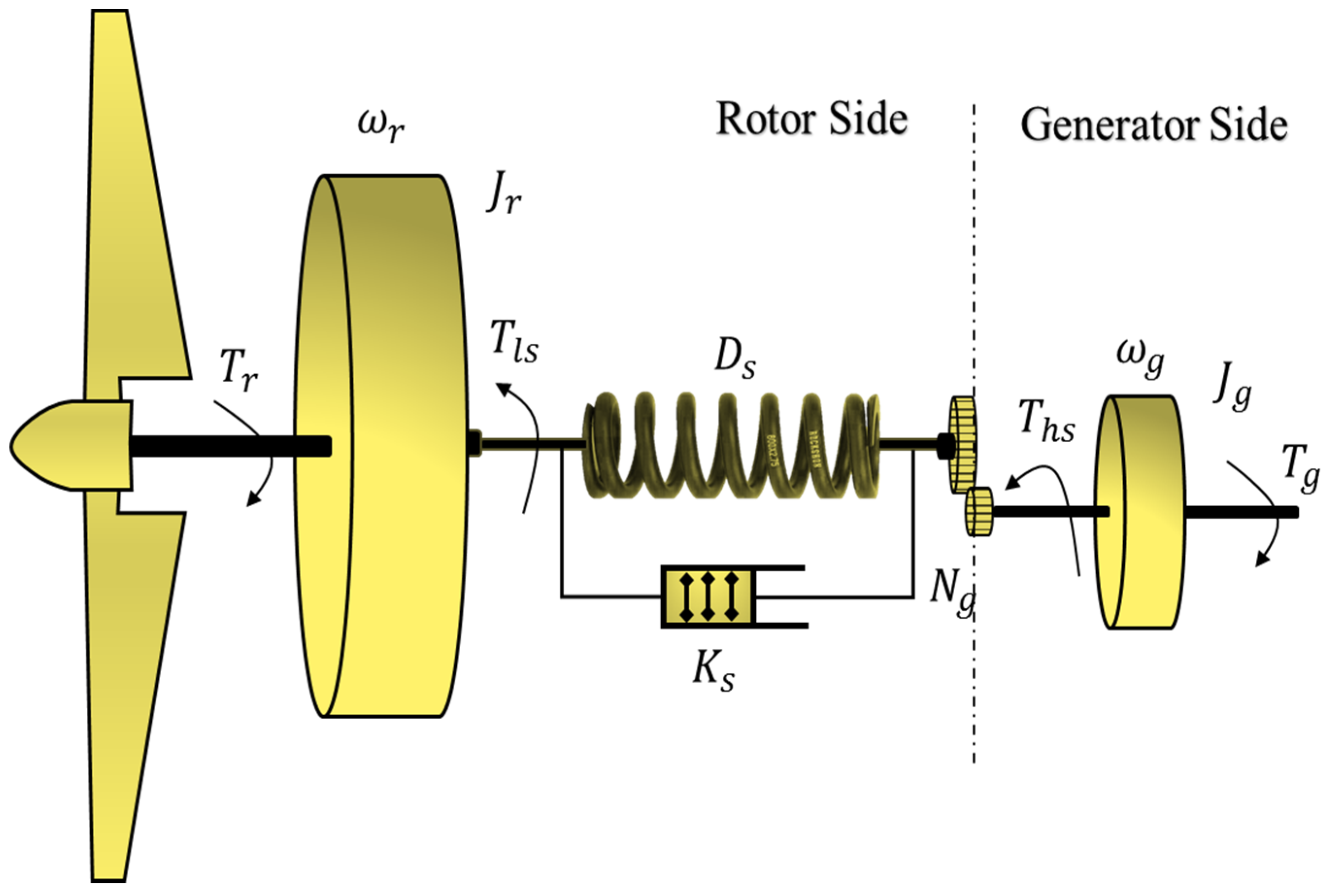
Figure 1. Structure of a typical wind turbine [28].
Designs 04 00015 g001
Figure 2. Illustration of nonlinear integral backstepping model-free control (NIB-MFC) loop control.
Designs 04 00015 g002
Figure 3. A proposed strategy for the combination of hardware-in-loop (HIL) and software-in-loop (SIL) testing.
Designs 04 00015 g003
Figure 4. Illustration of an actor–critic network.
Designs 04 00015 g004
Figure 5. Structure of the actor neural network (ANN) and critic neural network (CNN).
Designs 04 00015 g005
Figure 6. Step distribution of wind speed.
Designs 04 00015 g006
Figure 7. HIL output comparative results of backstepping controller based DDPG in combination with model free control (MFC), backstepping and PI controllers optimized by PSO according to Scenario I.
Designs 04 00015 g007
Figure 8. The trend of average reward in the HIL environment.
Designs 04 00015 g008
Figure 9. SIL output comparative results of backstepping controller based DDPG, backstepping controller based PSO and PI controller based PSO according to Scenario I.
Designs 04 00015 g009
Figure 10. The trend of average reward in the SIL environment.
Designs 04 00015 g010
Figure 11. Random distribution of wind speed.
Designs 04 00015 g011
Figure 12. HIL output comparative results of backstepping controller based DDPG, backstepping controller based PSO and PI controller based PSO according to Scenario II.
Designs 04 00015 g012
Figure 13. SIL output comparative results of backstepping controller based DDPG, backstepping controller based PSO and PI controller based PSO according to Scenario II.
Designs 04 00015 g013
Figure 14. Comparison of mean square error (MSE) and root mean square error (RMSE) standards for the parametric uncertainties.
Designs 04 00015 g014
Table 1. Settling time, overshoot and error comparison outcomes according to the Scenario I.
Performance MeasurementsDDPG Based NIB-MFCPSO Based NIB-MFCPSO Based PI
HILSILHILSILHILSIL
Settling time0.020.030.060.1521.623.2
Overshoot0.196%0.24%0.28%0.36%30.7%35.1%
Error0.0760.160.1780.2311.2113.92