Experimental and Numerical Investigation of Tip Leakage Flows in a Roots Blower

Abstract

Computational fluid dynamics (CFD) can help in understanding the nature of leakage flow phenomena inside the rotary positive displacement machines (PDMs). However, due to the lack of experimental results, the analysis of leakage flows in rotary PDMs by CFD has not yet been fully validated. Particle image velocimetry (PIV) tests with a microscopic lens and phase-lock were conducted to obtain the velocity field around the tip gap in an optical Roots blower. The three-dimensional unsteady CFD model of the Roots blower with the dynamic grids generated by Screw Compressor Rotor Grid Generation (SCORG) was established to predict the gap flow under the same operating conditions. The images obtained by the PIV tests were analyzed and some factors which compromise the quality of test results in the gap flow were identified, such as reflections and transparency of the window. The flow fields obtained by CFD have the same flow pattern and velocity magnitude as the experimental results in the majority of observed regions but overestimate the leakage flow velocity. The CFD results show a vortex induced by the leakage flow in the downstream region of the gap. The flow losses in the tip gap mainly happen at the entrance upstream of the gap. Finally, some suggestions for future work are discussed.

1. Introduction

Rotary PDMs such as screw machines, scroll machines, vane machines and Roots blowers are widely used for ranges of industrial applications. In all these machines, gaps between moving and stationary parts have to be maintained to ensure their safe and reliable operation. However, the gaps are desired to be minimal, because leakage flows play an important role in the performance. The leakage flow could reduce the discharge mass flow rate and increase the input power, which leads to the reduction of volumetric and indicated efficiency. There are many factors that have an influence on the leakage flow such as gap size, gap structure, pressure difference, fluid viscosity, flow pattern and wall velocity. Hence, it is difficult to predict the leakage flow rate accurately and establish the accurate simulation model of PDMs.

Many researchers have studied leakage flows through clearance gaps in rotary PDMs both experimentally and numerically. Numerical methods are mostly based either on the theoretical model [1,2] or CFD model [3,4,5]. In theoretical models, the nozzle model [1,6] is the most widely used, which simplifies any leakage channel as a nozzle. Thus, the leakage mass flow rate can be calculated with the isentropic flow equation in the nozzle. The adiabatic Fanno flow model [7] was developed including the friction loss of the leakage channel, in that the model is more accurate than the nozzle model. However, the correction coefficients which are added in both models to reduce the deviation are empirical and need to be verified by experiments.

As governing conservation equations such as mass, energy and momentum are solved numerically in CFD models, leakage velocities in gap paths can be obtained without any assumption. It is believed leakage mass flow rates obtained by CFD models are more accurate. In CFD models of PDMs, moving grids are essential since working chambers move and deform with crank angle. Therefore, how to generate high quality moving grids especially in gaps of PDMs is the key to conduct successful CFD simulation.

Roots blowers are a type of PDM that usually have two engaged rotors with two or more lobes in each. The rotors rotate in opposite directions within the casing and form working chambers between the rotors and casing. Roots blowers do not have internal compression, as the volume of the chamber remains constant while rotating. The increase of the pressure is caused by the backflow from the high-pressure side [8,9]. There are three kinds of gaps in Roots blower: the tip gap, the interlobe gap and the axial gap. Hence, the generation of moving grids in gaps is critical for the establishment of CFD model in Roots blower. Rane and Kovacevic [10,11,12] reported the latest moving mesh generation methods in PDMs in detail, which has been integrated into the commercial software SCORG. Grids can be generated in the main flow domain as well as the leakage domain of PDMs using SCORG and can be used by most of commercially CFD solvers, such as FLUENT, STAR-CCM+ and ANSYS CFX. Casari et al. [13] conducted the transient numerical analysis of the Roots blower using SCORG as mesh generator and Open FOAM as a solver. Their results provided the leakage flow field map in the tip gap. Liu et al. [14,15] and Sun et al. [16,17] established the CFD simulation model of the roots blower and validated it by measurements of mass flow rate and pressure distribution. Huang and Liu [18] conducted the analysis using 2D numerical meshes at various rotating positions for three-lobe twin-rotor Roots blower. Their results revealed the presence of highly transient flow mechanisms within the 2D flow field interacting with the radial and interlobe leakage flows for the Roots blower. Xing et al. [19] used TwinMesh and ANSYS-CFX to simulate a three-lobe Roots blower numerically and display the presence of strong vorticial flow field and backflow through three gaps. Joshi et al. [20] predicted the leakage flow rate in a two-lobe Roots blower using a stationary mesh in CFD at a single rotation angle and compared them with experimental data. A tip step which was also applied in the present study was used and was proved to reduce tip leakage of the Roots blower [20].

The accuracy of the CFD model depends on a lot of factors, such as the mesh, turbulence model and the flow solver [10,21]. Whether these CFD models can sufficiently capture the flow field in PDMs remains to be known. The CFD models in PDMs are usually validated by measuring integral parameters such as the total mass flow rate and power [12,14,16]. However, it is doubtful that the simulation leakage flow field is identical with the practical one when the simulated power or mass flow rate agrees with the test result. Unless the actual leakage flow velocities are measured, such CFD models cannot be fully validated. Therefore, for the full validation of numerical calculations, it is required to obtain accurate measurements of the flow field in the gap of rotary PDMs.

Some researchers have attempted to evaluate internal flows in PDMs using optical methods in the past. Sachs [22] investigated the gas flows in the tip gap of a static flat rotor screw compressor using the Toppler Schlieren method. The swirls and shocks in the tip gap were obtained. The influence of pressure ratio, gap shape, gap height and moving boundary on the leakage flow was studied and laser Doppler velocimetry (LDV) method was recommended to acquire quantitative results in the gap. Guerrato et al. [23] measured the flow field in the working chamber near the discharge chamber and in the discharge chamber of oil-free compressors using LDV while Kovacevic et al [24] measured the flow in suction chamber of the compressor. However, as the screw machines have the helical rotors that limit optical access to the flow field, the quantitative velocity values in working chamber domains and gap domains cannot be obtained. Sun et al. [9,25] and Singh et al. [26] measured the velocity in the working chamber of a Roots blower with straight lobes using optical methods and compared the unsteady simulated main flow fields with the PIV test results. The three-dimensional and unsteady nature of the flow field was illustrated and the leakage flows through the three gaps were discussed. In reference [26], the measured tip leakage flow was displayed without introducing the test rig for leakage flow and comparing with CFD results, so the validation of the leakage flow of the CFD model has not been fully achieved in the past and the leakage flow nature needs to be investigated further.

In this paper, microscopic PIV experiments were conducted to obtain the velocity field in the tip gap under different pressure ratios. The raw images are analysed first to find the factors that will influence the quality of test results. A three-dimensional unsteady CFD simulation model was established to predict the gap flow under the test operation conditions after the tip gap was calibrated with the high-resolution test images. The CFD results are compared with the test results and then are analysed to investigate the main flow and leakage flow in the Roots blower. The work of this paper will provide instructions for high precision PIV measurement of the gap flow and high fidelity of CFD simulation in order to study leakage flow mechanisms in rotary PDMs.

2. Experimental Study

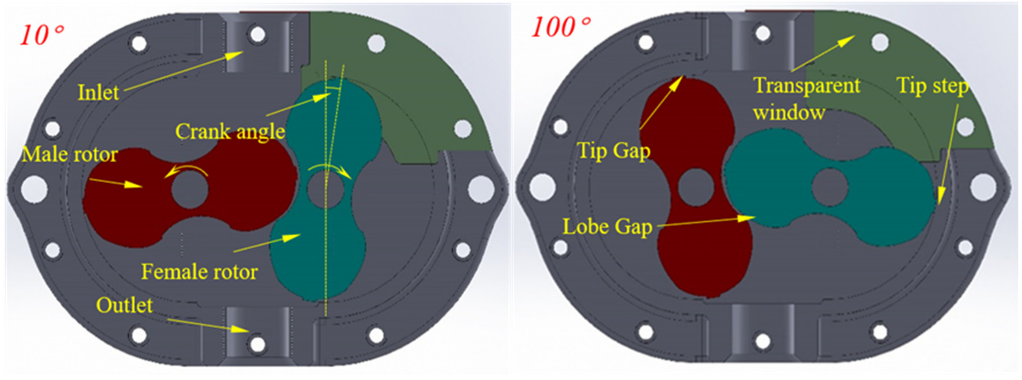
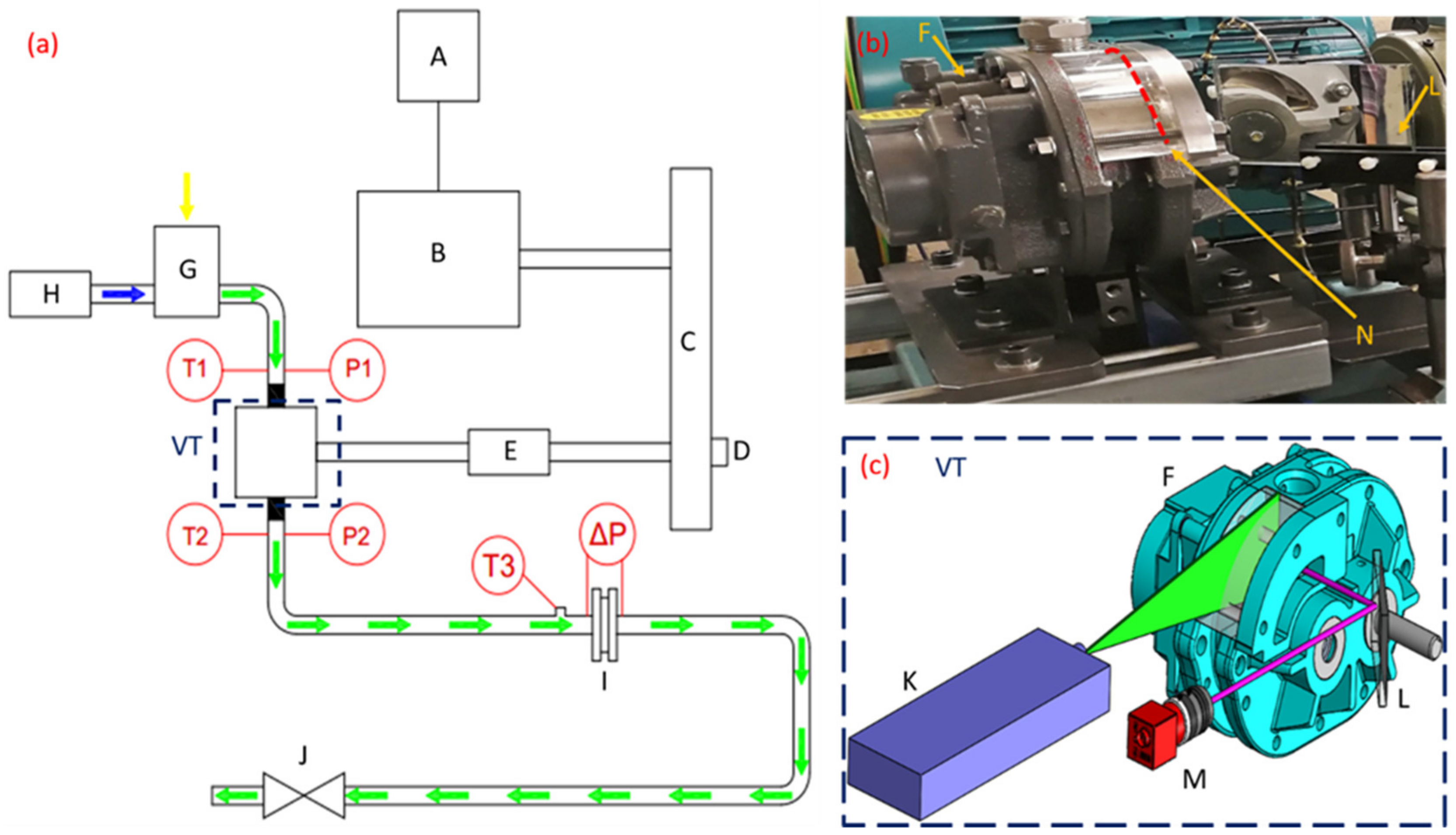
2.1. Experimental Setup and Data Processing

This paper studies a roots blower with two-lobed rotors mounted on parallel shafts that rotate in opposite directions to transfer air as working fluid. The physical model is shown in Figure 1. The suction and discharge pipes connect to the inlet and outlet domains respectively. The air passes into the roots blower through the inlet and fills into the suction chamber formed by the casing and rotor. The female rotor rotates clockwise, and the reference crank angle when the female rotor is vertical is defined as 0°. Three types of gaps are recognized in the Roots blower, namely the tip gap, the interlobe gap and the axial gap between the side of the lobes and the casing. The main dimensions are shown in

Table 1. The main geometrical parameters of the Roots blower.

Items	Specification	Items	Specification
Diameter of the rotor (mm)	101.3	Tip gap (mm)	0.4
Axis distance (mm)	63.12	Lobe gap (mm)	0.17
Rotor length (mm)	50.5	Axial gap (mm)	0.15
Displacement volume (L/rev)	0.4618	Width of tip step (mm)	6.4

.

Figure 2 provides details of the experimental test rig. The layout of the test rig is shown in Figure 2a. The tracking smoke was injected into a smoke tank (G) and mixed with the air in the tank. The optical Roots blower was fixed on the test rig and inhaled air from the smoke tank. The optical window was designed to allow optical access through two locations: the radial window and the side window (see Figure 2c). The flow field in the working chamber is captured through the side window using the reflection image in the mirror (L) in Figure 2c. The PIV method was employed to test the velocity flow field on the laser sheet plane (N) which was 5 mm inside the chamber from the side window (see Figure 2b). A shaft encoder (D) was mounted on the shaft to realize the phase-lock, which means every pair of images was taken at the same crank angle. The double-pulse laser (K) and double shutter camera (M) with the resolution of 2048 × 2048 pixels were used to take every pair of images at a short interval of 2–50 µs that was depended on the maximum particle velocity in the flow field. The equipment used for measurements was introduced in detail in the previously published paper by the authors [9,25,26].

For the measurement of gap flow field, following changes were made to the test set-up: Firstly, the microscope lens Model K2 (Infinity photo-optical, Centennial, CO, USA) was equipped on the double-shutter camera to magnify the tip gap (see Figure 3). The transparent window was polished to remove scratches and small pits on the surfaces. The female rotor, the bolts and inner surface of the casing were painted black to reduce the reflection of the laser. The original transparent window and the painted female rotor are shown in Figure 4.

The tests of tip leakage flow were conducted under two operating conditions as shown in

Table 2. Operating conditions for the Roots blower test

Inlet Pressure (Bar)	Inlet Temperature (K)	Outlet Pressure (Bar)	Outlet Temperature (K)	Pressure Ratio (-)	Speed (rpm)	Mass Flow Rate (g/s)
0.990	300.1	1.005	301.2	1.015	464	1.71
0.990	300.6	1.061	306.9	1.072	464	1.18

. The inlet was open to the atmosphere. The discharge pressure was controlled by a discharge valve. The speed and the operating pressure ratios were lower than the practical design parameters, as the transparent window cannot endure high pressure and high temperature. For every operating condition, images at two positions of the female rotor that were at a crank angle of 30 degree and 43° were captured. The time interval of the pulsed laser changed from 3 μs to 12 μs.

In every test case, 120 pairs of images were recorded by the camera with the resolution of 2048 × 2048 pixels. From every pair of images, the velocity can be processed out using the Adaptive PIV method in Dynamic Studio V6.4 (Dantec Dynamics, Skovlunde, Denmark). The adaptive PIV method is an automatic and adaptive cross-correlation method that iteratively adjusts the size and the shape of the individual interrogation areas (IA) in order to adapt to local seeding densities and flow gradient, further details of which could be found in [27]. And the detailed processing procedure for the images of gap flow is the same as that in a previous publication [26]. After processing a pair of images, the instantaneous velocity field were obtained. Then the average velocity field was calculated out by averaging many instantaneous velocity datasets at the same position in the test case.

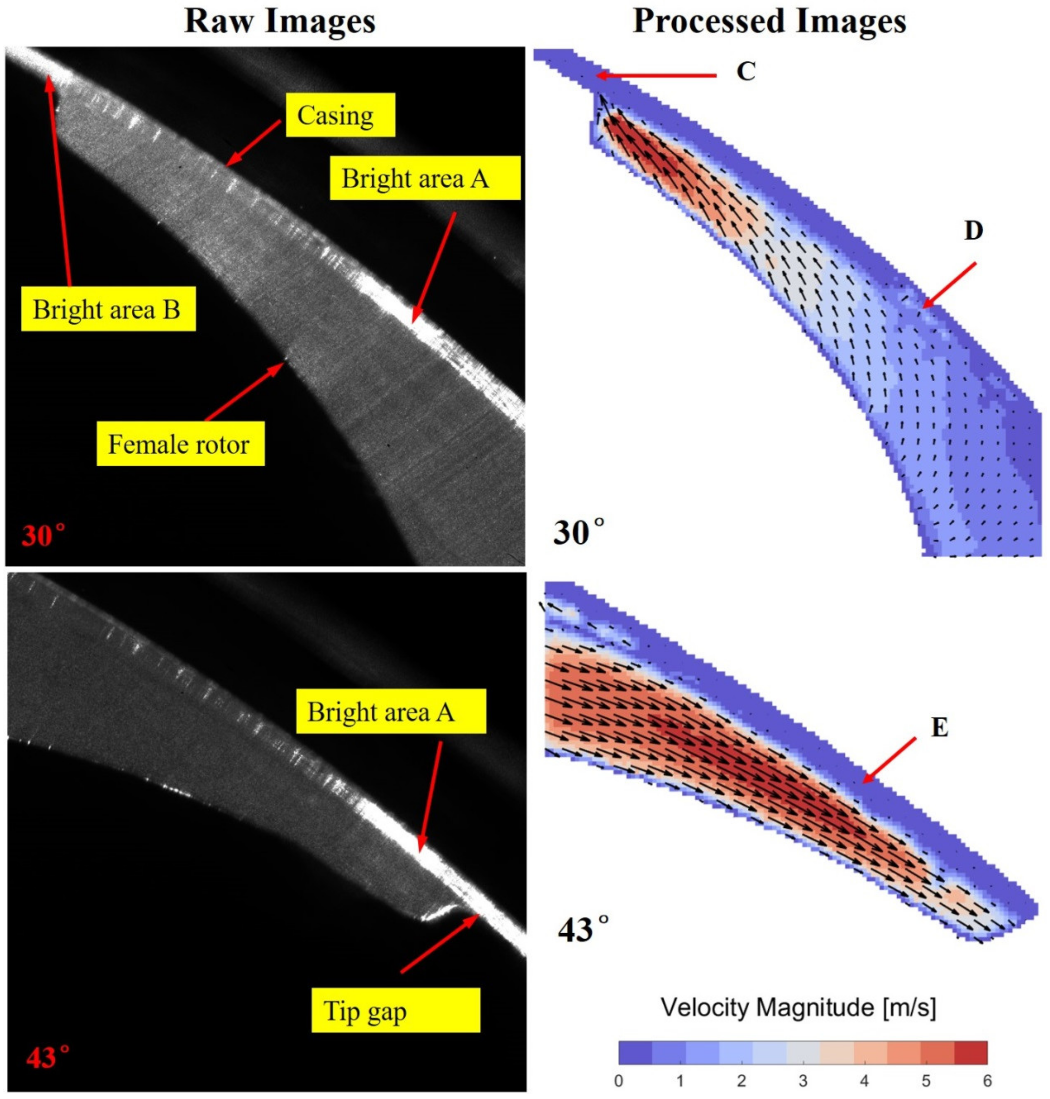
2.2. Experimental Findings

Figure 5 shows the raw and processed images at the crank angle of 30° and 43° when the pressure ratio is 1.015. The raw images are the first frame of one pair of images. The laser time interval was 6μs under two operating conditions. When the crank angle was 30°, the flow field in the image was upstream of the leakage flow through the tip gap. Moreover, the flow field at the crank angle of 43° was downstream of the tip-gap leakage. In the tip gap of both figures, the bright area A and B exist. Because the light intensity is so high in these areas, the PIV method is unable to calculate the flow velocity field in these overexposed regions. As a consequence, vectors near the casing in the processed images approach to zero, such as the area C, D and E, which deviates from the real velocity. There are two reasons for the formation of the bright area. One is the surface flaw near the casing, which caused light scattering. As the shot position of the camera was the same at the two crank angles, the casing and the transparent window in the two figures were the same. It is found that the bright area A existed in the same position in the two figures and did not move with the rotors. The pits or scratches in this area scattered the laser and made the area appear bright. It is also noticeable that the streak bright lines exist on the right of the bright area, which also resulted from the surface flaws of the transparent window near the casing. Therefore, the surface flaws have to be removed to achieve better quality in future measurements of the leakage velocity in the tip gap. Another reason for the bright area is the reflection of the rotors. The bright area B only happened at the crank angle of 30° when the tip-step of female rotor passed by it. The planar laser-induced fluorescence method (PLIF) can be used in future studies to eliminate the reflection of the surface.

Figure 6 shows the first frame of 7th and 8th pair of raw images at the same crank angle and pressure ratio. The phase-lock condition required every pair of images to be identical to each other at exact the same crank angle. However, the images change in angular position slightly from cycle to cycle because of fluctuations in the rotational speed [26]. We found that the images match each other after every 10 cycles. In Figure 6, the length of the tip step in one image can be measured. After the magnification factor which was 196.25 pixels/mm was divided, the length of L1 is about 0.7 mm shorter than that of L2. This corresponds to a jitter of about 0.78° crank angle. When the velocity field is obtained by processing the raw images, the masked figure which is generated by averaging the fluid domain of 120 raw images is used to cut out the boundary area for every pair of images. If the cycle to cycle fluctuation happens, the velocity near the boundary will have big deviations during the processing. And when the transient flow fields are averaged, the crank angle of the test changes and will be different from than the setting degree. For the gap flow PIV measurement, as the actual length of the measured area is only about 10mm, the cycle-to-cycle fluctuations result in large deviation of the average velocity field. In this test, it was deduced that the fluctuations were caused by the synchronizing gear. As shown in Figure 4, the transparent window was equipped as the casing of the female rotor which was driven by the synchronizing gear. The shaft encoder which sent the trigger signal to the laser instrument at the same position in a cycle was equipped on the shaft of the male rotor. The transmission deviation of the synchronizing gear leads to the fluctuations of the position of the female rotor. If the transparent window can be equipped on the male rotor side, the transmission deviation can be eliminated. Another method is to select one raw image in every ten samples, then process and average the selected images. It means that 5000 pairs of images need to be measured at one crank angle in order to obtain 500 pairs of identical images.

The tip gap size and shape play an important role in the tip leakage flow velocity. When generating the moving grids in rotor domain in SCORG, it is an essential parameter that will influence the accuracy of simulation results. The designed tip gap in this Roots blower is 0.1 mm. But the actual gap size will be very different. In this test, as the transparent window was manufactured to replace the raw casing and was polished several times to remove the scratches on the inner surface, the gap size would be larger than the designed value which is 0.1 mm. Hence, the tip gap size needed to be measured for the prediction of the leakage flow. The application of the microscopic lens offers the opportunity to measure gap size through visualization method. As shown in Figure 7, it is the local view of the tip gap at 43 degree in Figure 5. In the software, Photron FASTCAM Viewer 3.6.8.1 (Photron Limited, Tokyo, Japan) the length of the tip gap L3 can be measured in the raw image with the resolution of 2048 × 2048 pixels. Then the gap size can be calculated by dividing the magnification factor with the measured pixels of L3. As the magnification factor in this test was 196.25 pixels/mm, the measured deviation of L3 was reduced. The measured length of L3 is 78.5 pixels, and the gap size is 0.4 mm which has been added in Table 1.

When the pressure ratio of the Roots blower increased, the backflow increased simultaneously and the mass flow rate decreased. Because the tracer particles were generated by a smoke machine vaporizing a liquid glycol, the liquid particles had the chance to attach on the transparent widow and convert into droplets. Figure 8 shows the images under a pressure ratio of 1.072. The bright strip can be found in both raw figures and the bright dots can be spotted in the figure of 30°. At the dot or strip area and around them, the velocity vector cannot be processed out as the strip or dots covered particles. In the processed image of 30 degrees, no vector is shown in area F, which is caused by Bright strip A and droplets. In the processed image of 43 degrees, the velocity flow field around the rotor surface is interrupted by area G where the vectors are small and disordered, which is caused by Bright strip B. The strip and dots were caused by the concentrated liquid particles on the transparent window. As the speed of 464 rpm was low and the pressure ratio was high, the liquid particles cannot flow through Roots blower quickly and a number of particles keep stationery caused by the backflow and vortex, so the liquid particles concentrated on the surface of the window to form the droplets or film which caused the bad quality of the raw images. In these images, the velocity of particles near the film and droplets cannot be calculated correctly. During the test, once the phenomena happen, the test had to stop and the transparent window had to be dismantled and cleaned, which make it impossible to test under high-pressure ratio. One solution for this is to change the liquid particles into the solid particles. Another solution is to improve the rotational speed to enlarge the flow rate of the Roots blower.

3. CFD Model for Roots Blower

3.1. CFD Settings and Boundary Conditions

A CFD model was established to simulate the flow field of the Roots blower under the operating conditions in Table 2. The CFD settings are shown in

Table 3. CFD settings of the Roots blower.

Setting	Specification	Setting	Specification
Advection scheme	High-resolution	Turbulence numeric	1st order
Transient scheme	2nd order backward Euler	Wall model	No-slip with adiabatic walls
Turbulence model	SST k-w with automatic wall functions	Iteration per time step	20
Heat transfer model	Total energy including viscous terms	Inlet/Outlet condition	Opening with static pressure & temperature
Working fluid	Air as Ideal gas	Inlet turbulence intensity	5%
Domain initialization	Standard atmospheric conditions	Convergence criteria	RMS 1E-4
Time step at 464 rpm	3.592 × 10−4

below. The turbulence model was the shear stress transport (SST) k-w model with automatic wall functions. The SST turbulence model is the most prominent two-equation model, which was designed to give high accurate predictions of the onset and the amount of flow separation. One of the advantages of the formulation is the near-wall treatment for low-Reynolds number computations where it is more accurate and more robust [28]. Therefore, the model can handle the turbulent main flow and laminar boundary flow accurately. The turbulence intensity at the inlet was 5%. The CFD simulations were conducted under the operating conditions are shown in Table 2. So, the inlet and out pressure in Table 2 were used. The time step was calculated with the rotational speed when the rotor rotated by one degree.

3.2. Grid Generation and Grip Independence Study

As the tip gap has been calibrated, the casing to rotor conformal grids for the moving rotor domain were regenerated using in-house grid generation software SCORG v5.7 [10,11,12] with tip gap of 0.4 mm. The stationary meshes in the fluid domains for inlet and outlet chambers and pipe were generated in ANSYS Mesh [9]. Then the grid independence study was conducted on rotor grids. Four levels of rotor grids were generated according to the standard procedure provided in reference [29]. The grid number of every level is controlled by circumference, radial and axial divisions [30]. Each division of the next grid level was 1.414 times of that of the present level. Therefore, the grid size of the next level increased by 2.828 times [29]. The grid levels and number divisions are shown in

Table 4. Grid levels and number divisions.

Level	Circumference	Radial	Angular	Axial	Number of Grid Cells in Rotors
Grid-1	200	15	180	18	216,000
Grid-2	285	21	180	25	600,600
Grid-3	400	30	180	35	1,680,000
Grid-4	500	38	180	44	3,344,000

. It can be noticed that the cell number of Grid-4 is about 2 times of that of Grid-3 because the case with grids of 2.82 times of Grid-3 ran too slowly in our workstation. As the paper focuses on the tip leakage flow, the average outlet mass flow rate and the tip leakage flow rate at the crank angle of 90 degrees were output to check the grid independence. As shown in Figure 9. Both the average outlet mass flow rate and the tip leakage flow rate decreased with rotor grid cell number. When the rotor grid number increased from Grid-3 to Grid-4, the mass flow rate and the tip leakage flow rate decreased by 0.5% and 1%, respectively. Therefore, the Grid-3 was selected as a grid-independent mesh and was used for further analysis in this paper.

4. Analysis of the Tip Leakage Flow

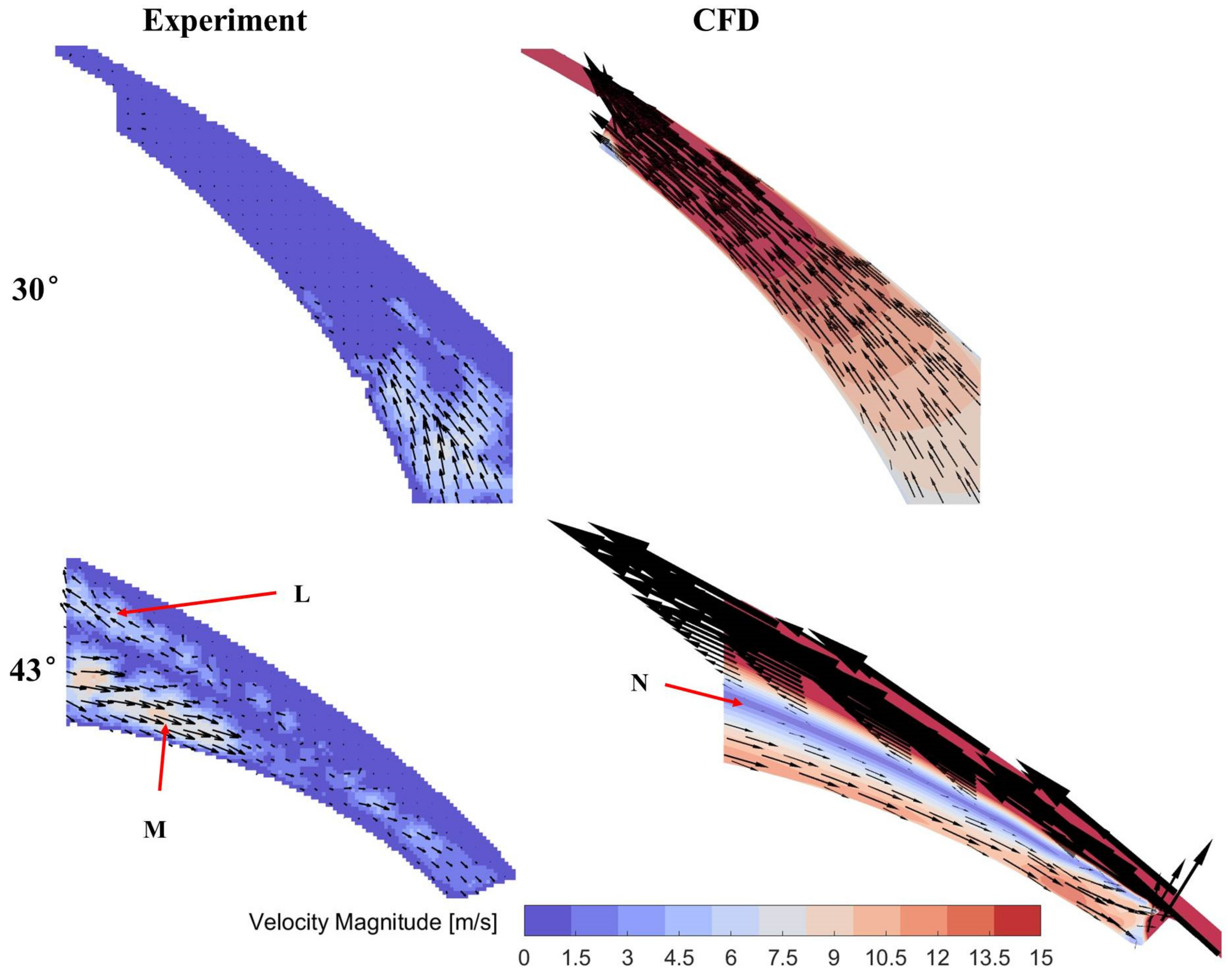
4.1. Comparison between the Experimental and Simulation Results

Figure 10 and Figure 11 show the velocity magnitude contours superimposed by the velocity vectors for both simulation and experimental results near the tip gap under pressure ratios of 1.015 and 1.072, respectively. The colourmap of experimental and CFD results show the velocity magnitude in the plane of the laser sheet. The experimental results are averaged from unsteady velocity vectors in the measured cycles.

In Figure 10, the velocity direction and magnitude at 30 degrees have been predicted well by the CFD model except for the area H where the particle velocity cannot be tested correctly. The fluid flows back into the tip gap under the pressure difference across the tip gap. In the CFD image of 43 degrees, high-velocity leakage flow from the tip gap happens near the casing, which actually has a maximum velocity of 43 m/s. When the simulated velocity is higher than 20 m/s, the larger velocity vectors are hidden to keep low-velocity flow field legible and the whole figure clear. The simulated flow pattern is similar to the experimental pattern. The fluid at area I flows towards the tip step while the backflow happens near the casing. Although the experimental flow field near the casing cannot be calculated out due to the bright area shown in Figure 6, the backflow can be identified by the vectors at area J. In the CFD image of 43 degrees, there is a low-velocity area labelled by K. The area forms because of the mixture of the fluid with opposite velocity direction. The low-velocity area also exists on the experimental figure, but only the area below the area J can be seen clearly and most of the area was not captured by the test. However, it can be deduced from the experiment figure that the low-velocity area is narrower than the area K and is closer to the casing. It suggests that the experimental velocity of leakage flow is lower than the simulation one and will not spread over a large area like the simulation results. One reason for the overestimation of the leakage velocity in CFD simulation is that the actual pressure difference may be lower than the simulation value. Because outlet pressure is close to the atmospheric pressure, the fluctuation of the outlet pressure will bring large deviation of the pressure ratio when the outlet pressure in the test was obtained by averaging 10–15 times of acquired data. Continuous acquisitions of the inlet and outlet pressure will be helpful to provide the accurate pressure value for CFD simulation.

In Figure 11, the experiment and CFD velocity fields near the tip gap under the pressure ratio of 1.072 are compared. It is noticeable that the colourmap ranges from 0 to 15 m/s, which is larger than the test results under the pressure ratio of 1.015. At 30°, the CFD model predicts the same flow direction with the test but overestimates the velocity magnitude. In the CFD image of 43 degrees, the velocity vectors which are higher than 55 m/s are hidden, and the maximum velocity reaches 104m/s. At the crank angle of 43°, the flow pattern of simulation results almost matches with the experimental value. The velocity direction and magnitude at area M coincide with the simulation results. The low-velocity area N also happens at the same position in the experiment image. The experiment results capture the backflow more clearly at area L than that at the pressure ratio of 1.015. But the velocity magnitude is far lower than the simulation value in this area. It indicates that the simulation results overestimate the downstream velocity. At high-pressure ratio, the backflow has larger velocity and flow rate. So, it is possible that the seeding particles crash each other and accumulate together to become big particles. As shown in Figure 8, some droplets form during the test. As the big particles or droplets have larger density and viscosity than air and cause larger flow loss in the tip gap, the test leakage velocity will be lower than the CFD results which did not consider the influence of the liquid particles.

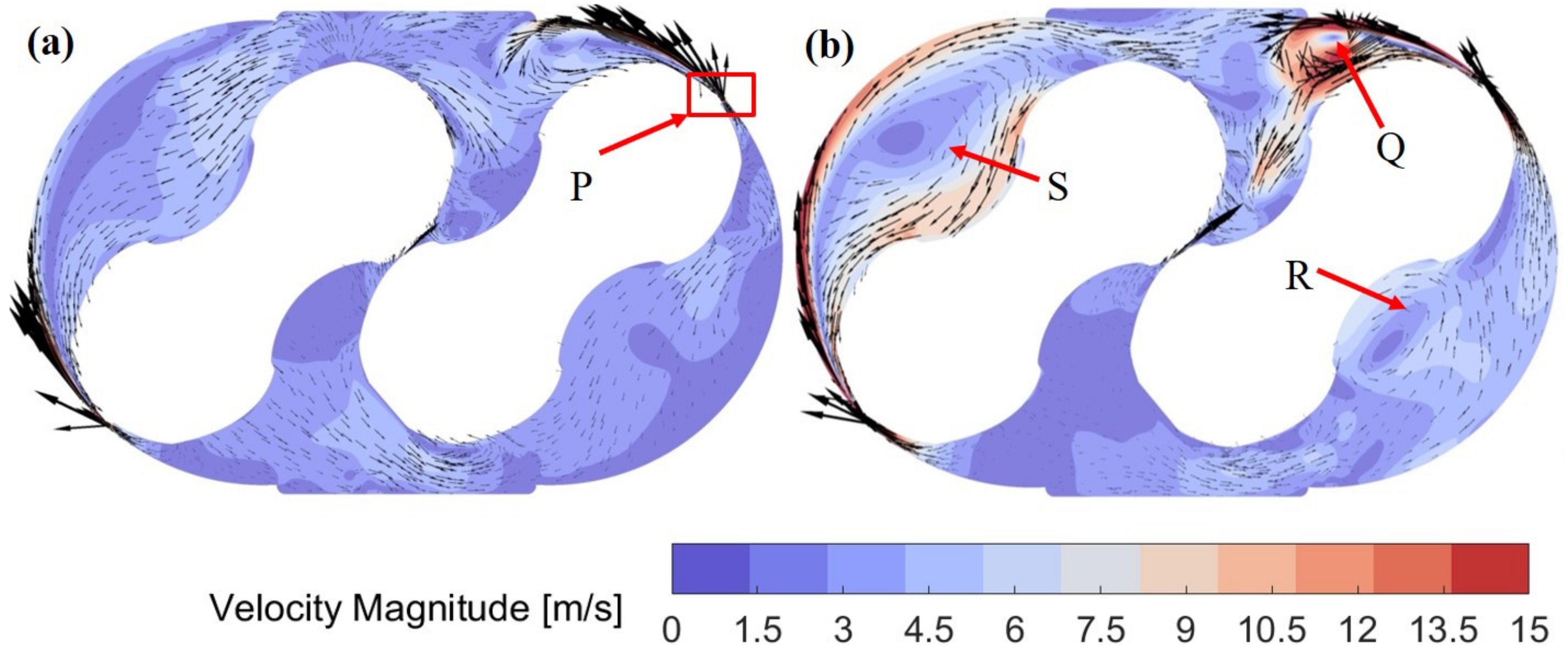
4.2. Analysis of the Overall Flow Field

Figure 12 shows the overall flow field on the laser plane at the crank angle of 43° under the pressure ratio 1.015 and 1.072, respectively. As shown in Figure 10 and Figure 11, the high-velocity areas (I, M) exist along the rotor surface in front of the tip step at the crank angle of 43°. As the velocity is far higher than the rotor velocity, it is not caused by the movement of the rotor. Figure 12 shows that the tip leakage flows along the casing and then turns around to flow along the surface of the rotor. So the high-velocity areas (I, M) in Figure 10 and Figure 11 forms under the effect of the tip leakage and the main flow near the inlet port. Meanwhile, the vortex Q happens at the downstream of the tip gap in Figure 12 under both pressure ratios. The low-velocity area (K, N) belongs to the vortex. As the high-velocity area (I, M) and low-velocity area (K, N) also exist in experimental results, there should be a vortex at the downstream of the tip gap caused by the leakage flow in the real flow. When the pressure ratio increases, the mass flow rate decreases. However, the main flow and leakage flow velocity increases after comparing Figure 12a and Figure 12b. The flow pattern also changes with the pressure ratio. In Figure 12b, the backflow from the outlet travels along the casing and toward the tip gap. Part of the backflow turns around and forms the vortex R. At the same time, the tip leakage in the right chamber flows far away from the gap and forms the vortex S under high-pressure ratio. In contrast, both vortices do not form under the pressure ration of 1.015 as shown in Figure 12a, because the backflows from the outlet and the tip leakage have low velocity and cannot influence the main flow field intensively. Hence, the main flow filed is influenced significantly by the tip leakage flow.

Figure 13a is the magnification view of the area P in Figure 12a. And the rotation was done to make the view horizontal. The tip step is marked in this figure. Then the total pressure field, the static pressure field and velocity field in the tip gap at the crank angle of 43° under the pressure ratio 1.015 are displayed in Figure 13. The variation of velocity profile along the tip gap under the pressure ratio of 1.005 can be seen in Figure 13a. The fluid begins to accelerate at the entrance of the tip gap. At the ‘central face’ of the tip gap, the velocity profile becomes stable and changes a little along the gap channel. The maximum velocity is 43 m/s which is at the upper half of the velocity profile at the central face. The asymmetrical velocity profile is caused by the asymmetrical inlet shape. The rotor velocity also influences the shape of the velocity profile, but the influence is very limited as it is far lower than the leakage velocity. At the outlet of the tip gap, the leakage flow does not diffuse with the enlargement of the space after the tip step, which is caused by high-velocity flow ‘I’ as shown in Figure 10. The reduction of total pressure in Figure 13b represents the flow loss in the tip gap. It can be seen that the flow loss mainly happens at the entrance of the tip gap. Along the gap channel, the total pressure reduction is caused by the friction loss of the boundary. At the exit of the gap, the total pressure does not fall abruptly as the leakage flow does not diffuse. Hence, the new designation can be done at the tip step to increase the flow loss in the channel and at the exit of the gap. Figure 13c shows the static pressure field in the tip gap. The static pressure decreases along the gap channel. However, the low-pressure area and the adverse pressure gradient exist on the surface of the tip step at the entrance, the central plane and the outlet of the tip gap. There are two reasons for the formation of the low-pressure area. The rotor rotates clockwise, which causes the larger flow loss on the wall of the tip step is larger, so both the total pressure and the static pressure on the wall is low. When the fluid flows around the chamfer and the center of tip step, it is accelerated and the static pressure decreases.

At the high-pressure ratio of 1.072, the variation of the velocity profile, the total pressure and the static pressure are similar to that at the pressure ratio of 1.014, as shown in Figure 14. The maximum velocity increases from 43 to 104 m/s due to the increase of pressure ratio. The average velocity at the central face can be calculated out using the integral method. They are 33 m/s and 76 m/s under the two pressure ratios respectively. The Reynolds number with the gap size as the characteristic length is 1790 under the pressure ratio of 1.072, so the flow in the gap is laminar flow. Because of the laminar flow, the velocity improvement on the surface of tip step is higher than that on the top of gap at the chamfers and the center of tip step, which causes the low-pressure areas and the radial static pressure gradient.

The practical leakage flow in the gap should also be the laminar flow as the test leakage velocity is lower than the CFD results. If the nozzle model [1,6] is used for the prediction of the average leakage velocity, the predicted velocity will be higher than CFD results because the nozzle model does not consider that the friction flow loss and the flow loss at the entrance of the tip gap. So the flow coefficient needs to be added in the nozzle model to modify the prediction. If the velocity in the tip gap can be measured with PIV experiment, the flow coefficient can be determined accurately.

5. Discussion

The objective of the project is to study leakage flow mechanisms using experimental and numerical methods and finally to reduce leakage and improve the performance of rotary machines. The double-shutter PIV test was done to measure the velocity field in and around the tip gap in a Roots Blower. The unsteady CFD simulation model was established based on the deforming meshes. There are a series of factors that influence the test results in the gap, such as the surface flaws of the transparent window, the reflection of the surface, the transmission error of the synchronized gear, the accumulation of the liquid particles and the pressure fluctuation. Each factor will lead to the deviation of the measured results even the failure of the test. The solutions to these problems have been provided in Section 2 and Section 3, and additional work needs to be performed for future measurements. It can be found that the transmission error, the accumulation of liquid particles and the pressure fluctuation are related to the movement of the rotors. For the static test, the pressure will be stable, and no variations due to vibrations and transmissions would occur. Also, the pressure ratio can be controlled easily and will be more stable, the flow rate can be larger and the flow direction will not change frequently. The liquid particles will not concentrate and form droplet easily. Hence, the static benchmarking test is recommended to be completed in the future studies. The movement of the tip step actually does not influence the velocity profile inside the gap, because its flow speed is low relative to the leakage velocity. But the interaction between the leakage flow and the main flow still influence the flow field remarkably such as the high-velocity area I and M in Figure 10 and Figure 11. The high-velocity flow prevents the diffusion of the leakage flow at the exit of the tip gap as shown in Figure 13 and Figure 14. Therefore, the dynamic test is necessary to capture these features while designing tip shapes. In the future, the PLIF test on the static rotor can be done first after the transparent window is polished near the casing. Then the test rig for the rotating rotor can be redesigned to deal with the problems for high precision PLIF measurement of the gap flow.

For the simulation, it is essential to confirm the gap size and the boundary conditions, because they have an important influence on the leakage flow. It is shown that the leakage flow still has a larger velocity along the casing boundary after the exit of the tip gap in Figure 9, Figure 10 and Figure 12. It means that the velocity gradient at the boundary of the casing is big. Hence, it is necessary to refine the mesh at the boundary of the casing to keep the local Y-Plus lower than 1 for the SST turbulence model. In addition, if the CFD model could consider the influence of particles using multiphase model, the accuracy will be improved.

6. Conclusions

The following conclusion can be derived from the analyses on the experimental and simulation gap flow results in the Roots blower:

(1)

A series of factors deteriorating the results of the PIV test were observed as follows: the surface flaws of the transparent window, the reflection of the surface, the jitter in the phase-locking due to uncertainties in the transmission of the synchronized gear, the accumulation of the liquid particles and the pressure fluctuations. These factors caused an increase in erroneous vectors and limited the quality of measured velocity fields. The solutions to these problems were discussed and will be implemented in future measurements in our lab.

(2)

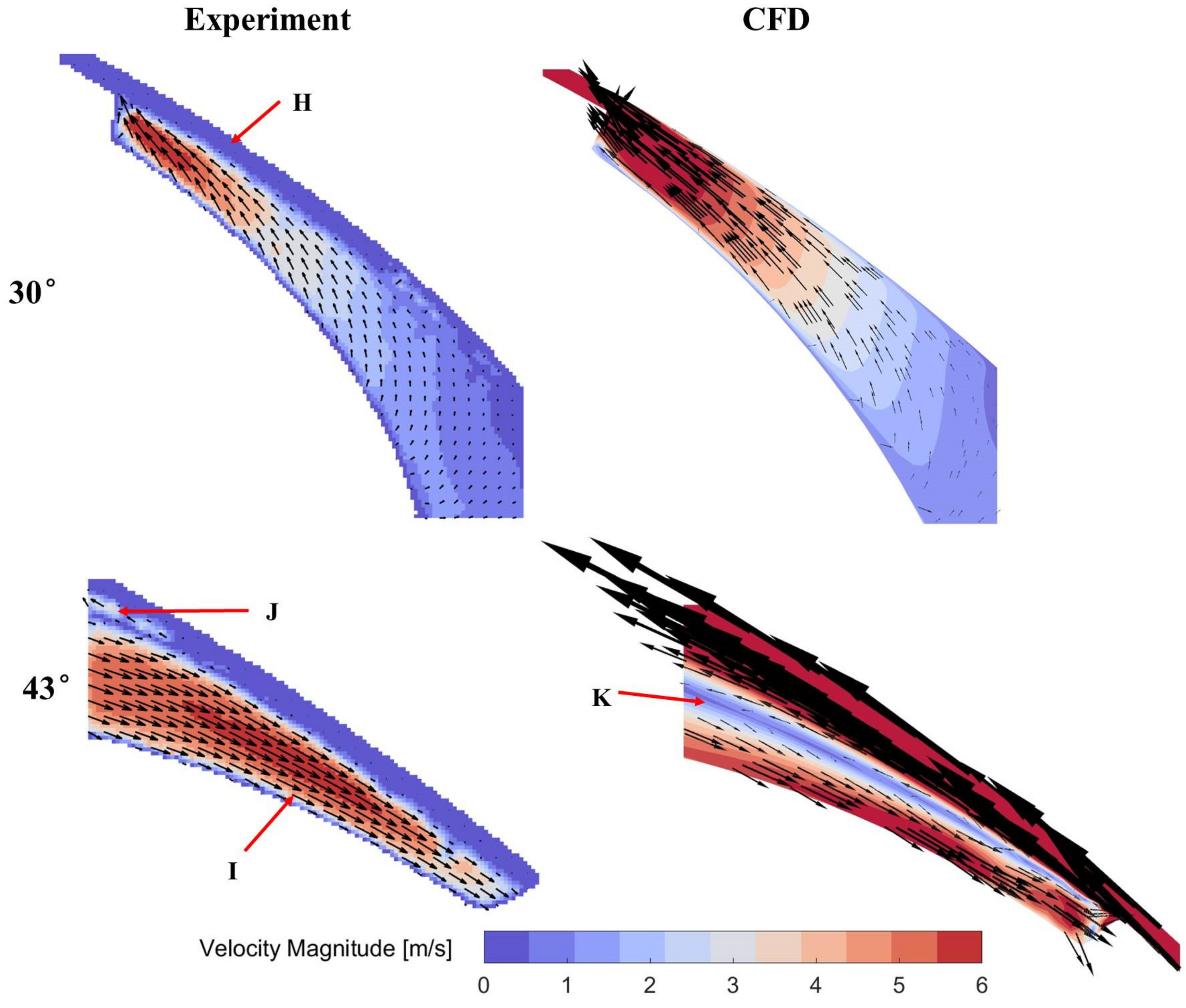
The CFD flow field agrees with experimental results in the flow pattern and velocity magnitude at certain areas but overestimates the leakage flow velocity.

(3)

The vortex induced by the leakage flow through the tip gap results in the separation of high and low-velocity areas in the downstream region of the leakage flow. The main flow field changes significantly with the increased pressure ratio.

(4)

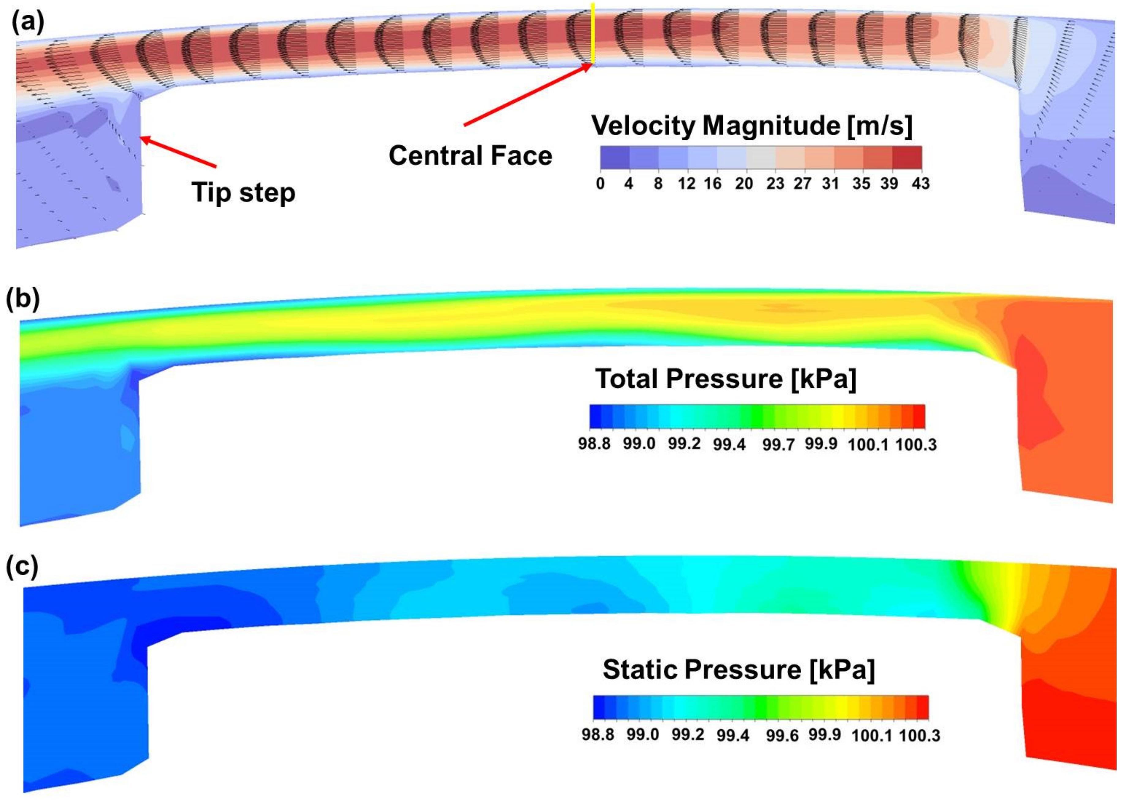
The leakage flow in the tip gap is laminar under the pressure ratios in this paper. The main flow losses occur upstream at the entrance of the tip gap. The total pressure changes moderately along the gap since the leakage flow does not diffuse much. The step at the rotor tip can be redesigned to increase pressure losses and reduce the leakage flow.

References

1. Fujiwara, M.; Mori, H.; Suwama, T. Prediction of the Oil Free Screw Compressor Performance Using Digital. In Proceedings of the International Compressor Engineering Conference 1974, Purdue University, West Lafayette, IN, USA, 10–12 July 1974; p. 119. [Google Scholar]
2. Stošić, N.; Smith, I.K.; Kovačević, A. Screw Compressors: Mathematical Modelling and Performance Calculation; Springer: Berlin, Germany, 2005. [Google Scholar]
3. Kovačević, A. Boundary adaptation in grid generation for CFD analysis of screw compressors. Int. J. Numer. Methods Eng. 2005, 64, 401–426. [Google Scholar] [CrossRef]
4. Kovačević, A.; Stošić, N.; Smith, I.K. Screw Compressors—Three-Dimensional Computational Fluid Dynamics and Solid Fluid Interaction; Springer: Berlin/Heidelberg, Germany; New York, NY, USA, 2007. [Google Scholar]
5. Sun, S.H.; Wang, X.W.; Guo, P.C.; Wu, K.; Luo, X.Q.; Liu, G.B. Numerical analysis of the transient leakage flow in axial clearance of a scroll refrigeration compressor. Proc. Inst. Mech. Eng. Part E J. Process Mech. Eng. 2019. [CrossRef]
6. Chen, Y.; Halm, N.P.; Groll, E.A.; Braun, J.E. Mathematical modeling of scroll compressors—Part I: Compression process modeling. Int. J. Refrig. 2002, 25, 731–750. [Google Scholar] [CrossRef]
7. Yanagisawa, T.; Shimizu, T. Leakage losses with a rolling piston type rotary compressor. I. Radical clearance on the rolling piston. Int. J. Refrig. 1985, 8, 75–84. [Google Scholar] [CrossRef]
8. Ucer, A.S.; Celik, I. Analysis of Flow through Roots Blower Systems. In Proceedings of the International Compressor Engineering Conference 1980, Purdue University, West Lafayette, IN, USA, 23–25 July 1980; p. 319. [Google Scholar]
9. Sun, S.; Kovačević, A.; Brücker, C.; Leto, A.; Singh, G.; Ghavami, M. Numerical and Experimental Analysis of Transient Flow in Roots Blower. IOP Conf. Ser. Mater. Sci. Eng. 2018, 425, 012024. [Google Scholar] [CrossRef]
10. Rane, S. Grid Generation and CFD Analysis of Variable Geometry Screw Machines. Ph.D. Thesis, City University of London, London, UK, 2015. [Google Scholar]
11. Rane, S.; Kovačević, A. Algebraic generation of single domain computational grid for twin screw machines Part I—Implementation. Adv. Eng. Softw. 2017, 107, 38–50. [Google Scholar] [CrossRef] [Green Version]
12. Kovačević, A.; Rane, S. Algebraic generation of single domain computational grid for twin screw machines Part II—Validation. Adv. Eng. Softw. 2017, 109, 31–43. [Google Scholar] [CrossRef] [Green Version]
13. Casari, N.; Pinelli, M.; Suman, A.; Kovačević, A.; Rane, S.R.; Ziviani, D. Full 3D Numerical Analysis of A Roots Blower with Open-Source Software. In Proceedings of the International Compressor Engineering Conference 2018, Purdue University, West Lafayette, IN, USA, 9–12 July 2018; p. 2620. [Google Scholar]
14. Liu, X.M.; Lu, J.; Gao, R.H.; Xi, G. Numerical Investigation of the Aerodynamic Performance Affected by Spiral Inlet and Outlet in a Positive Displacement Blower. Chin. J. Mech. Eng. 2013, 26, 957–966. [Google Scholar] [CrossRef]
15. Liu, X.M.; Lu, J. Unsteady Flow Simulations in a Three-lobe Positive Displacement Blower. Chin. J. Mech. Eng. 2014, 27, 575–583. [Google Scholar] [CrossRef]
16. Sun, S.K.; Zhao, B.; Jia, X.H.; Peng, X.Y. Three-dimensional numerical simulation and experimental validation of flows in working chambers and inlet/outlet pockets of Roots pump. Vacuum 2017, 137, 195–204. [Google Scholar] [CrossRef]
17. Sun, S.K.; Jia, X.H.; Xing, L.F.; Peng, X.Y. Numerical study and experimental validation of a Roots blower with backflow design. Eng. Appl. Comput. Fluid Mech. 2018, 12, 282–292. [Google Scholar] [CrossRef]
18. Huang, Z.; Liu, Z. Numerical study of a positive displacement blower. Proc. Inst. Mech. Eng. Part C J. Mech. Eng. Sci. 2009, 223, 2309–2316. [Google Scholar] [CrossRef]
19. Xing, L.; He, Y.; Wen, J.; Peng, X. Three-Dimensional CFD Modelling of a Roots Blower for Hydrogen Recirculation in Fuel Cell System. In Proceedings of the International Compressor Engineering Conference 2018, Purdue University, West Lafayette, IN, USA, 9–12 July 2018; p. 2562. [Google Scholar]
20. Joshi, A.; Blekhman, D.; Felske, J.; Lordi, J.; Mollendorf, J. Clearance Analysis and Leakage Flow CFD Model of a Two-Lobe Multi-Recompression Heater. Int. J. Rotating Mach. 2006, 2006, 1–10. [Google Scholar] [CrossRef] [Green Version]
21. Kovačević, A.; Rane, S.; Stosic, N.; Jiang, Y.; Lowry, S.; Furmanczyk, M. Influence of Approaches in CFD Solvers on Performance Prediction in Screw Compressors. In Proceedings of the International Compressor Engineering Conference 2014, Purdue University, West Lafayette, IN, USA, 14–17 July 2014; p. 2252. [Google Scholar]
22. Ronald, S. Experimental Investigation of Gas Flows in Screw Machines. Ph.D. Thesis, University of Dortmund, Dortmund, Germany, 2002. [Google Scholar]
23. Guerrato, D.; Nouri, J.M.; Stosic, N.; Constantine, A.; Smith, I.K. Flow measurements in the discharge port of a screw compressor. Proc. Inst. Mech. Eng. Part E J. Process Mech. Eng. 2007, 222, 201–210. [Google Scholar] [CrossRef]
24. Kovačević, A.; Arjeneh, M.; Rane, S.; Stosic, N.; Gavaises, M. Flow Visualization at Suction of a Twin Screw Compressor. In Proceedings of the International Screw Compressor Conference 2014, Dortmund, Germany, 23–24 September 2014; pp. 309–318. [Google Scholar]
25. Sun, S.H.; Kovačević, A.; Bruecker, C.; Leto, A.; Ghavami, G.; Rane, S.; Singh, G. Experimental Investigation of the Transient Flow in Roots Blower. In Proceedings of the International Compressor Engineering Conference 2018, Purdue University, Chicago, IL, USA, 9–12 July 2018; p. 2615. [Google Scholar]
26. Singh, G.; Sun, S.; Kovacevic, A.; Li, Q.; Bruecker, C. Transient flow analysis in a Roots blower: Experimental and numerical investigations. Mech. Syst. Signal Process. 2019, 134, 106305. [Google Scholar] [CrossRef]
27. Raffel, M.; Willert, C.; Kompenhans, J. Particle Image Velocimetry: A Practical Guide; Springer: Berlin/Heidelberg, Germany, 1998. [Google Scholar] [CrossRef]
28. Ansys Inc. ANSYS CFX Modeling Guide, Release 18.0; Ansys Inc.: Canonsburg, PA, USA, 2017. [Google Scholar]
29. Coleman, H.; Stern, F. Uncertainties and CFD code validation. J. Fluid Eng. 1997, 119, 795–803. [Google Scholar] [CrossRef]
30. PDM Analysis Ltd. SCORGTM Help Manual, V5.7; PDM Analysis Ltd.: London, UK, 2019. [Google Scholar]
Figure 1. Physical model of Roots blower at crank angle 10° and 100°.
Designs 04 00003 g001
Figure 2. Roots blower test rig and diagram of visualizing test: (a) Layout of the test rig, (b) The laser plane on the Roots blower, (c) Diagram of visualizing test. A—inverter, B—electromotor, C—pulleys, D—shaft encoder, E—torque meter, F—Roots blower, G—smoke tank, H—smoke machine, I—orifice plate, J—valve, K—Light source, L—surface mirror, M—double shutter camera, N—Position of Laser plane, T1—suction temperature transducer, P1—suction pressure transducer, T2—discharge temperature transducer, P2—discharge pressure transducer, T3—upstream temperature transducer, ΔP—differential pressure across an orifice plate.
Designs 04 00003 g002
Figure 3. Roots blower test rig with microscope lens.
Designs 04 00003 g003
Figure 4. The original transparent window and the painted rotor.
Designs 04 00003 g004
Figure 5. The raw and processed images under the pressure ratio of 1.015.
Designs 04 00003 g005
Figure 6. The first frame of the 7th and 8th pair of images.
Designs 04 00003 g006
Figure 7. The measurement of the tip gap size.
Designs 04 00003 g007
Figure 8. The raw and processed images under the pressure ratio of 1.072.
Designs 04 00003 g008
Figure 9. Rotor grid independence study.
Designs 04 00003 g009
Figure 10. Comparison between the PIV and CFD gap flow fields under the pressure ratio of 1.015.
Designs 04 00003 g010
Figure 11. Comparison between the flow fields in gaps obtained by experimental PIV and numerical CFD under the pressure ratio of 1.072 at two different angles of rotation (30o and 43o).
Designs 04 00003 g011
Figure 12. The overall flow field on the laser plane at 43° under pressure ratio 1.015 (a) and 1.072 (b).
Designs 04 00003 g012
Figure 13. The velocity and pressure distribution in the tip gap at the crank angle of 43° under the pressure ratio of 1.015: (a) velocity field, (b) Total pressure, (c) Static pressure.
Designs 04 00003 g013
Figure 14. The velocity and pressure distribution in the tip gap at the crank angle of 43° under the pressure ratio of 1.072: (a) velocity field, (b) Total pressure, (c) Static pressure.
Designs 04 00003 g014