Article

Numerical Study of Customised Mesh for Twin Screw Vacuum Pumps

Centre for Compressor Technology, City, University of London, London EC1V 0HB, UK
*
Author to whom correspondence should be addressed.
Designs 2019, 3(4), 52; https://doi.org/10.3390/designs3040052
Submission received: 17 October 2019 / Revised: 18 November 2019 / Accepted: 27 November 2019 / Published: 2 December 2019
(This article belongs to the Section Mechanical Engineering Design)

Abstract

:
The market for dry vacuum pumps is expected to increase in the coming years. Improving the efficiency of these machines requires comprehensive understanding of the flow dynamics within the working chambers. For this purpose, Computational Fluid Dynamics (CFD) is used as it offers better insight of the working process of a screw machine. In this study, a twin-screw vacuum pump with a large helix angle was analysed. This is a challenging case for CFD due to the limitations of grid generation in the transverse plane on the mesh quality. Two types of transverse meshes were generated using the software SCORGTM: casing to rotor non-conformal mesh and casing to rotor conformal mesh. The quality of the mesh in terms of aspect ratio and orthogonality were compared. The casing to rotor conformal mesh was used with ANSYS Fluent in order to obtain performance characteristics of the vacuum pump with the moderate helix angle of 62° such as the mass flow rate, rotor torque, and indicated power. The performance prediction results were satisfactory but the grid quality was relatively low with orthogonality reaching 40° and aspect ratio over 250 in some cases. As the helix angle increases the quality of mesh decreases. This paper presents the new development of a grid generation algorithm which uses the normal rack to map the fluid domain in the normal plane instead of the transverse plane. This new mesh generation method is expected to better align the computational grid with the main and leakage flows in order to significantly improve grid quality and reduce the numerical diffusion in case of screw machines with large helix angles.

1. Introduction

The first vacuum dry pumps based on the roots principle were introduced in 1984 in Japan [1]. Nowadays, the vacuum pumps are widely used in many different industries such as nanotechnology, microelectronics, medicine, pharmaceuticals, thermonuclear power, food and packaging industry and others [2]. The semiconductor industry is one of the largest and most rapidly developing markets for twin-screw vacuum pumps. Twin-screw vacuum pumps are positive displacement machines consisting of a meshed pair of screw rotors within the casing. The working principle of twin-screw vacuum pumps is as follows; with the rotation of the rotors, the gas is induced in the pump and subsequently trapped in the working chamber between the rotors and casing. Then it is transported towards the discharge where it is exhausted from the machine. To minimise contamination, twin-screw vacuum pumps are normally oil-free. The screw rotors are synchronised by timing gear, which ensures that they do not come into contact with each other. Both main and gate rotors commonly have the same profile comprising of a single lobe in order to reduce manufacturing cost as well as to achieve higher volumetric efficiency.
In order to improve the performance of twin-screw machines, it is important to fully understand the working process within the chamber. The performance characteristics can be calculated numerically through a 1D chamber thermodynamic model and 3D Computational Fluid Dynamics (CFD) numerical simulation. The 3D computational fluid dynamic simulation can give a better insight into the flow parameters of screw machines. The challenge for the CFD simulation of twin-screw vacuum pumps is the discretisation of the chamber volume which is between the moving rotors and a stationary housing. The applied numerical grids need to move, slide, and deform. Moreover, the geometrical complexity of helix rotors results in the rapidly changing gap size from the compression chamber to the clearances. Even though some CFD software packages are available to generate numerical mesh for the screw compressor geometry, they need considerable effort in order to achievesatisfactory results. In 2000, Kovacevic [3] described a first version of an independent stand-alone numerical grid generation software SCORGTM (Screw Compressor Rotor Grid Generation) written in FORTRAN to generate high quality numerical grid of an oil-free screw compressor. Analytical transfinite interpolation is employed for the generation of a suitable numerical mesh for screw machines with a boundary adaptation method, smoothing and orthogonalisation. This was a breakthrough as prior to this there were no techniques available to generate robust grids for twin-screw machines. These original grids were of the rotor to casing type generated using an algebraic grid generation method. Boundary points in the rotor to casing mesh are fixed to the rotor for the duration of the cycle making the numericalgrid on each of the rotors to rotate together with the rotor. Such a mesh accurately represents both rotor and casing but deforms in the region between the rotors to form the moving interface between two rotors. In addition, the boundary cells on the casing deform from hexahedral to other shapes as two or more vertices collapse to reture the cusp line between the rotor bores. This may not be suitable for performance calculation with all commercial CFD solvers.
Based on the feature of the rotor to casing type grid generated from Kovacevic [4] and the hybrid differential method form similar to Vande Voorde [5], Rane et al. [
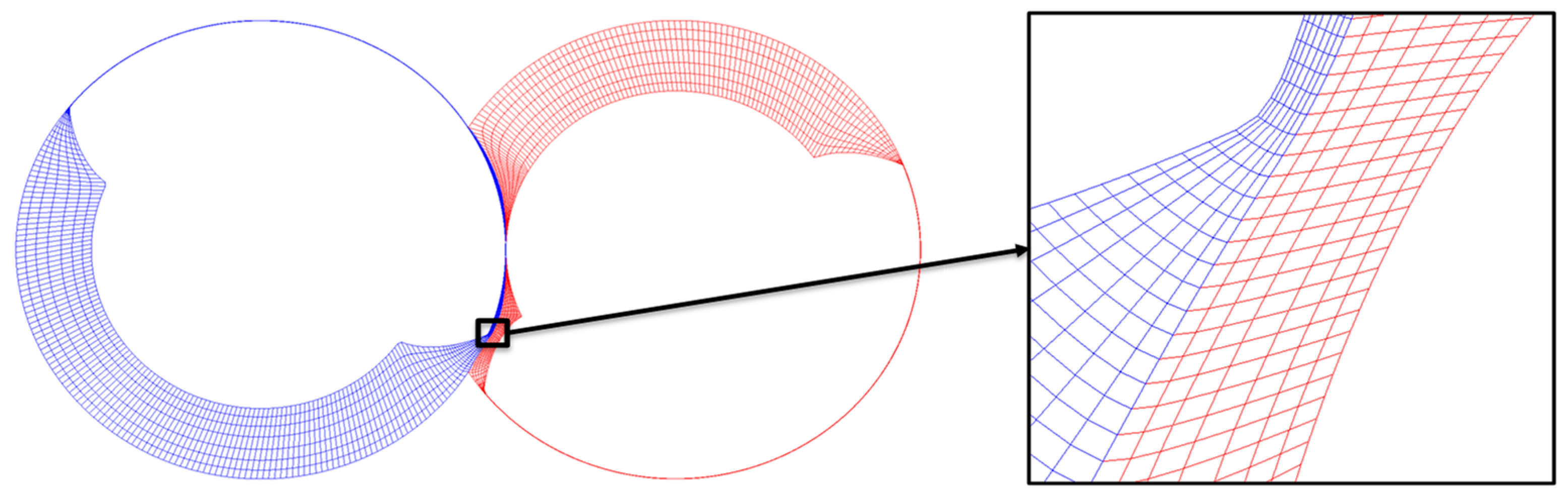
6] proposed new developments. Firstly, to introduce the grid generation called casing to rotor where boundary nodes are first positioned on the outer casing. These nodes remain unchanged relative to the rotors. The inner rotor nodes are distributed with reference to the outer nodes. Rotor nodes slide on the profiles as the rotor rotates. Such a grid structure is referred to as the Casing to Rotor grid type. Later on, with improving the interface region between two blocks by using combined algebraic and differential methods the conformal casing to rotor mesh was achieved [7]. Rane et al. [8,9,10] generated numerical mesh and conducted 3D simulation on the variable geometry rotors and multiphase screw machines. Kennedy et al. [11] presented a study of an oil-free twin-screw compressor using SCORGTM to generate conformal numerical mesh and ANSYS CFX 3D CFD tool [12] to calculate performance. This was compared with the validated 1D thermodynamic model. The paper concludes that the difference between both models decrease as the compressor operating speed increases. Hsieh [
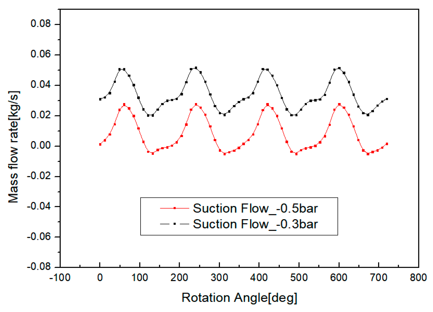
13] compared the 3D numerical results of cylindrical and screw type roots vacuum pumps using the CFD solver PumpLinx™ [14] assuming atmospheric inlet pressure. The results show that the cylindrical type pump has higher efficiency, while the screw type pump has a lower fluctuation in mass flow rate. This confirmed that numerical meshes generated by the method used in SCORG
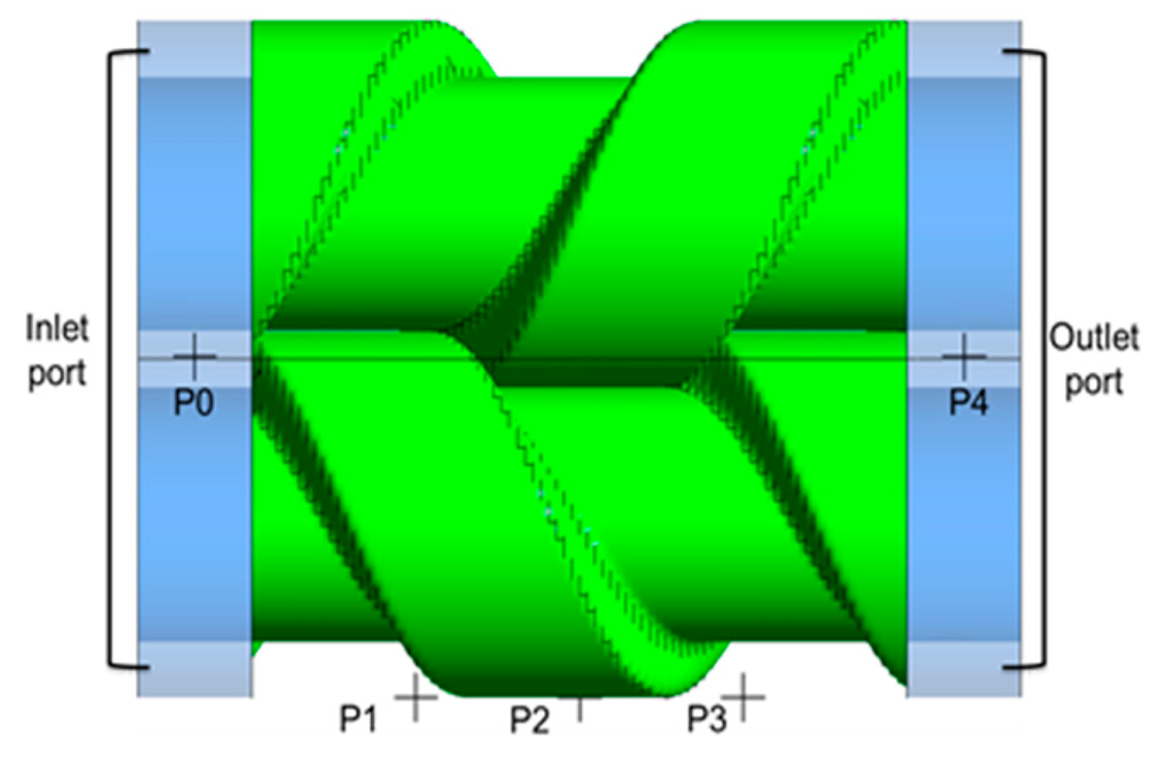
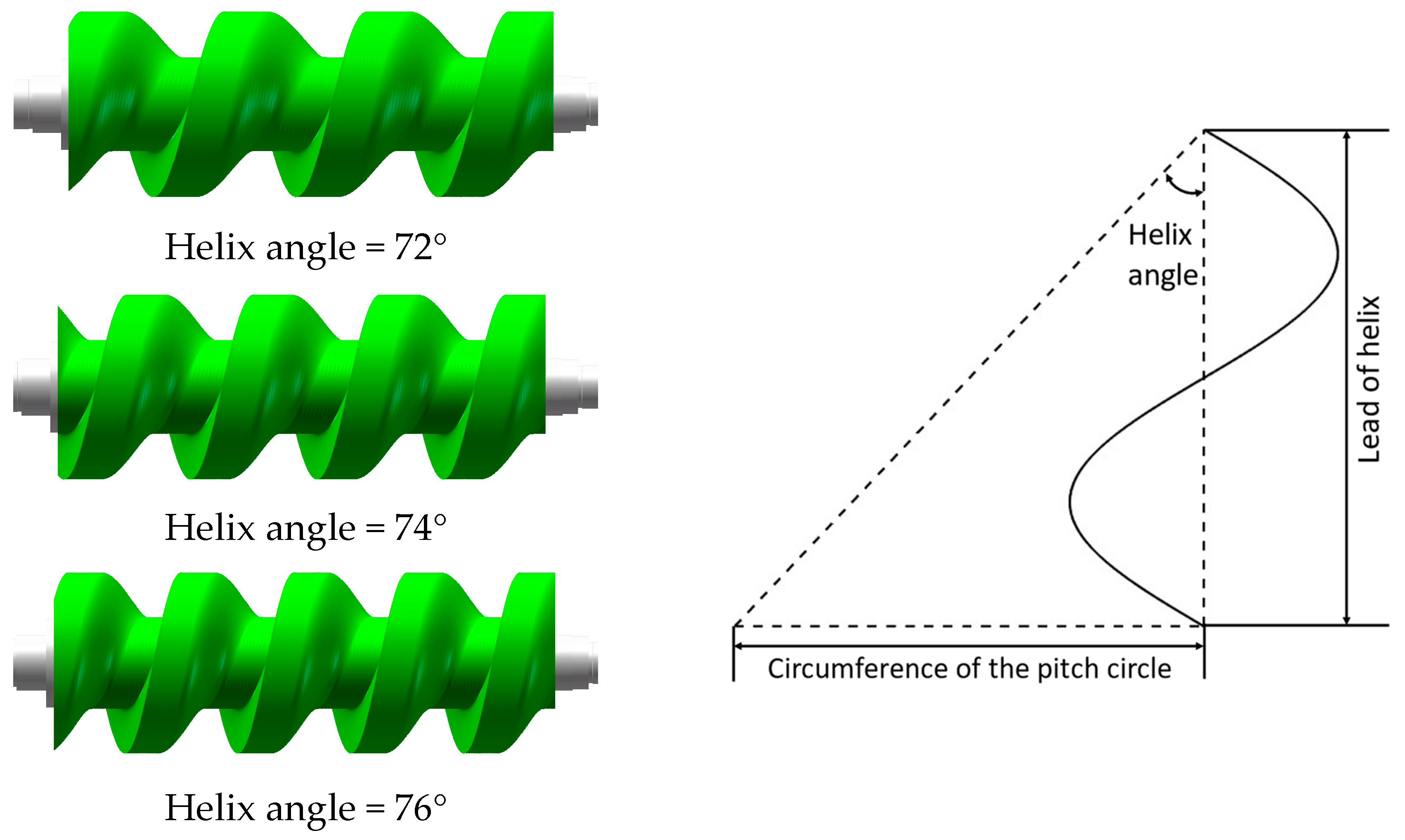
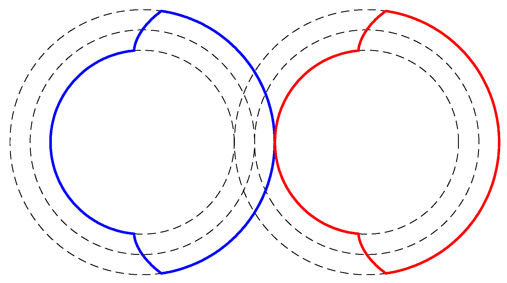
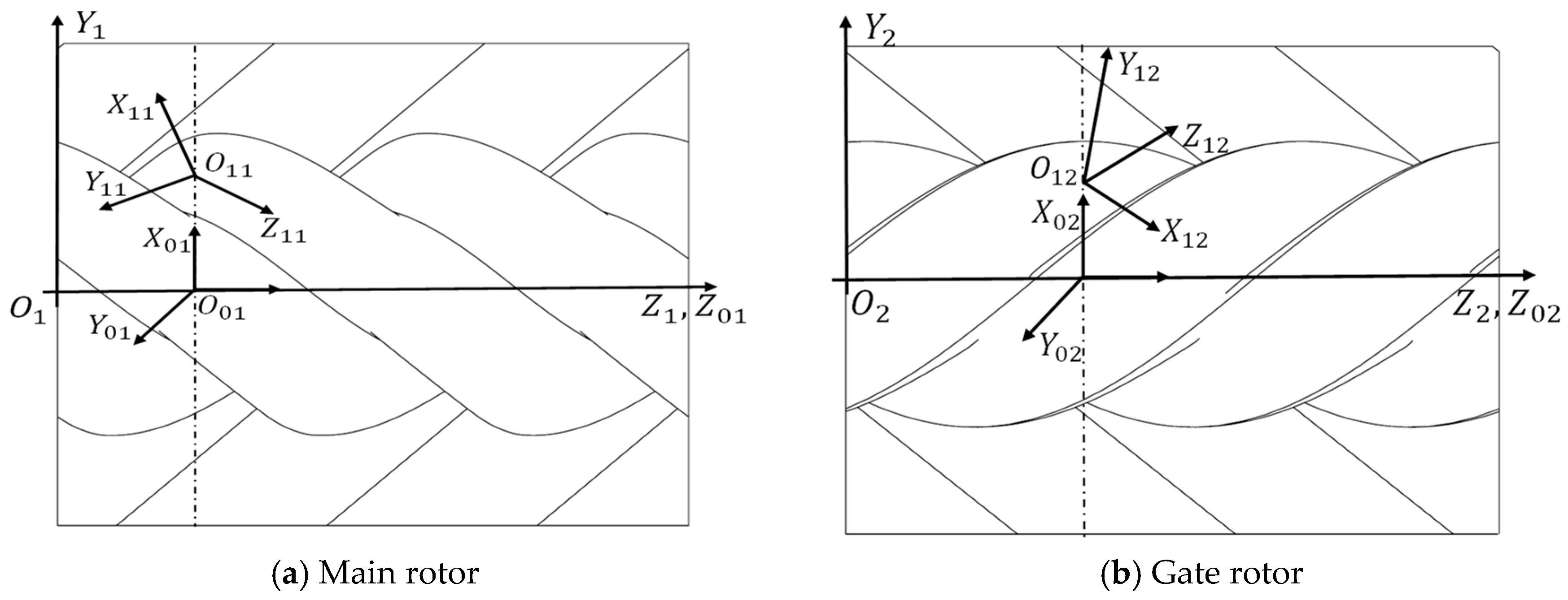
TM based on generation of series of 2D meshes in transverse planes either as rotor to casing or casing to rotor could be successfully used with a variety of CFD solvers. However, these meshes become difficult to use in calculation of the performance of vacuum pumps. There are two reasons for this, (a) the large helix angle as shown in Figure 1 will make the rotor to casing numerical mesh extremely non orthogonal which in turn leads to difficulty in obtaining CFD results and (b) in deep vacuum the continuum principle applied in the methods used in standard CFD codes will not apply.
Similarly, experimental study of twin-screw vacuum pumps under vacuum conditions is challenging due to the large size of the high precision vacuum pressure transducers required, and the difficulty of sealing these transducers when mounted in the casing. Tuo [15] conducted the experimental study on the working performance of one twin-screw vacuum pump under the working condition of 4 kPa suction pressure at 2700 rpm and 3000 rpm rotational speeds. So far, there is no published work on the 3D CFD simulation of a twin-screw vacuum pump under vacuum conditions. The mathematical models and software which were originally developed for twin-screw compressors can be effectively employed to simulate performance in twin-screw vacuum pumps [
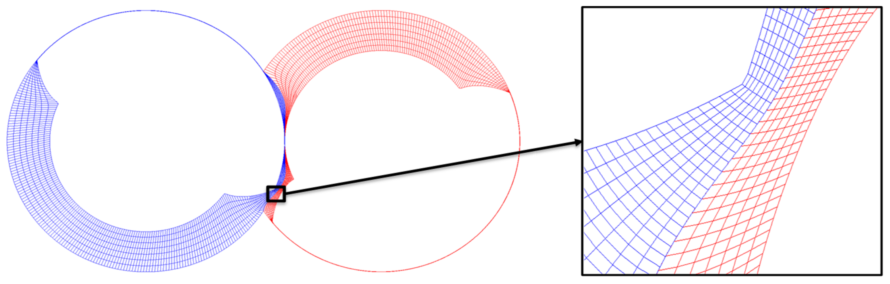
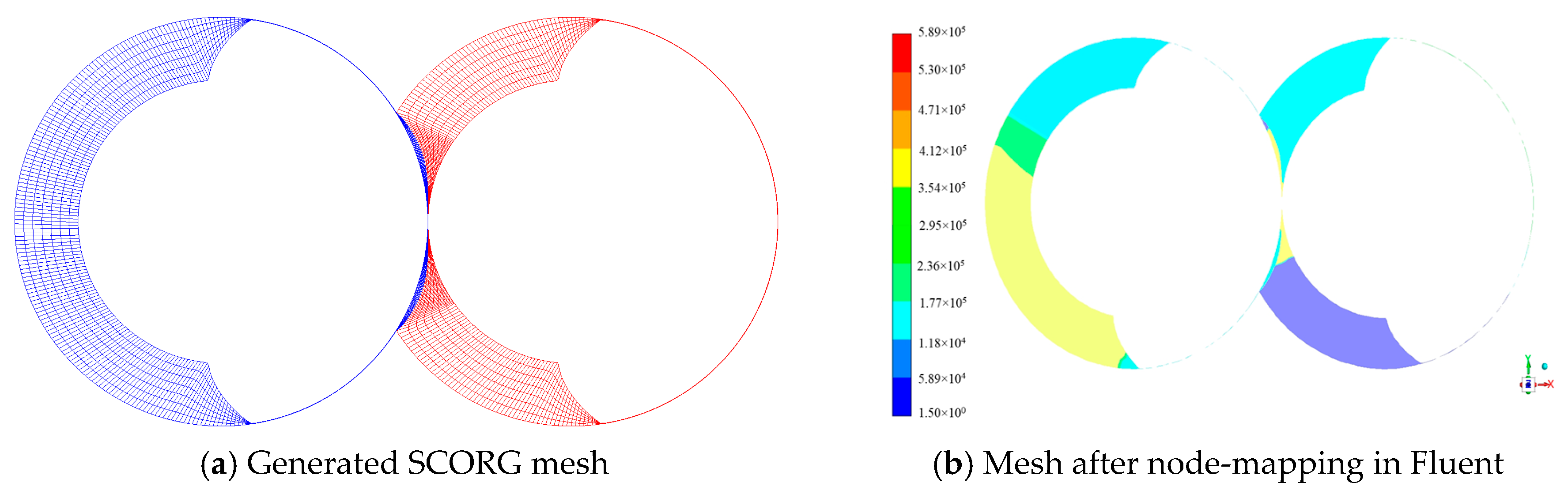
16]. In this study, a typical twin-screw vacuum with the moderate helix angle in low vacuum conditions is studied. Two different type of meshes are generated with the existing grid generation method, namely casing to rotor and rotor to casing mesh. This is used to compare the quality of grids. The casing to rotor conformal mesh is then used with the Fluent solver to obtain performance predictions using parallel processing.
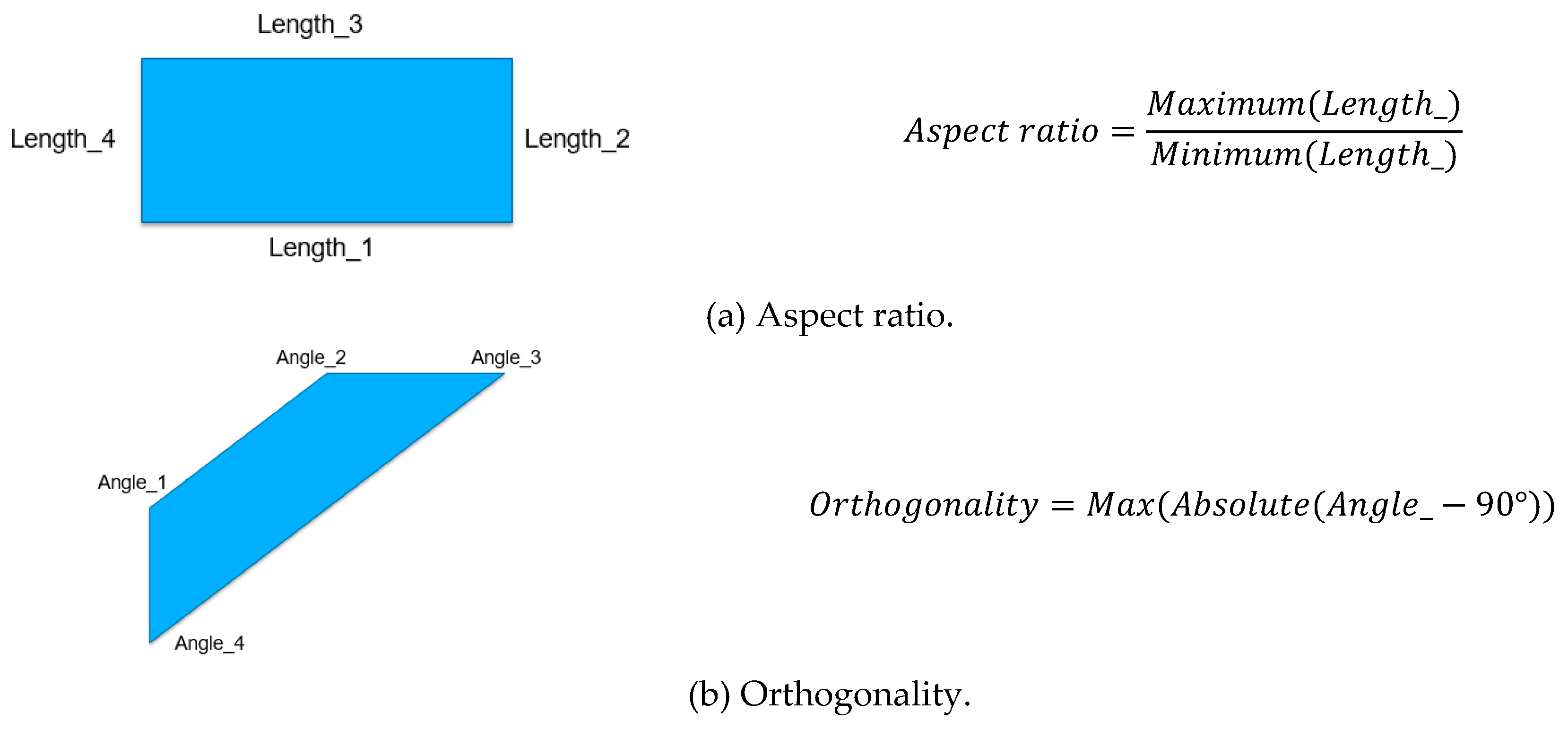
It was concluded that the current grid generation methods used for mapping of twin-screw machines could be used, but for the large helix angle vacuum pumps the quality of the grid may not be sufficient for accurate performance calculation. Since the grid is generated in the transverse plane the cells become highly nonorthogonal which leads to the numerical error when calculating fluxes through boundaries. According to the CFD study of twin-screw machines [17,18], the main fluid direction is perpendicular to the helix line especially in the clearance area. In addition, the numerical mesh in clearances is not aligned to the main direction of the leakage flow which causes numerical diffusion in clearances. As shown in 
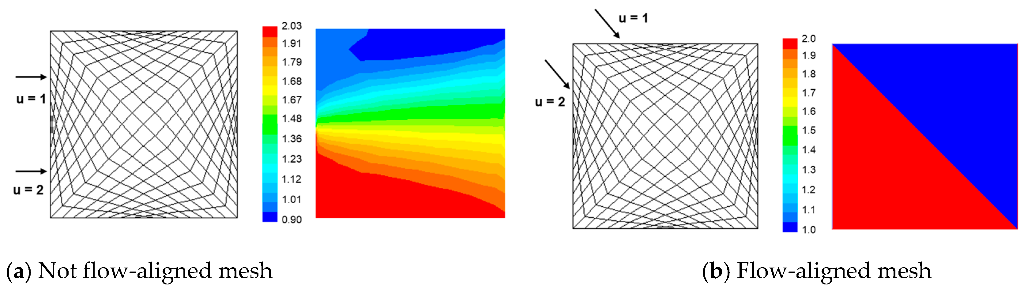
Figure 2, Vierendeels [19] evaluated effects which the grid alignment of structured numerical meshes to the direction of the flow has on numerical diffusion of 1st and 2nd order numerical schemes to solve transport equation. When the grid is not aligned to the flow direction as shown in Figure 2a, both 1st order and 2nd order numerical schemes will result in numerical diffusion which reduces with the mesh refinement. However, if the numerical grid is aligned to the direction of the flow, such as in 
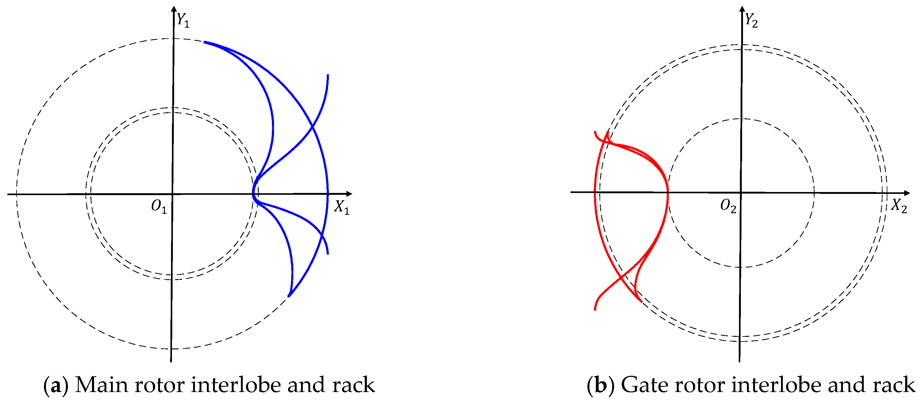
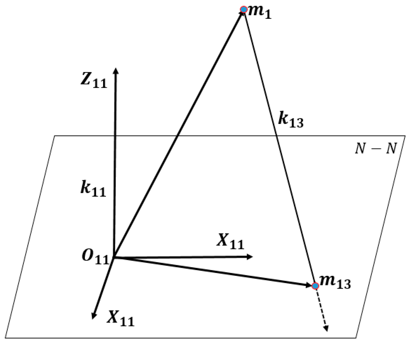
Figure 2b, than there will be no numerical diffusion and the prediction of velocities would be more accurate. This is very important for accurate prediction of leakage losses which are the main factor for efficiency of screw machines. Due to that, a different grid generation method using the normal rack procedure will be for the first time proposed in this paper. Both the main and the gate rotor coordinates will be first transformed to their normal plane, respectively, and the numerical grids will be generated in normal planes which are perpendicular to the helix line in the pitch circle of each desired normal cross section. This process is expected to make two major differences, (a) the numerical mesh will be nearly orthogonal and (b) the grid lines will be aligned to the flow through the clearances. This is expected to reduce numerical diffusion and increase accuracy and speed of calculation significantly.

2. Grid Generation for Twin-Screw Vacuum Pump

This section of the paper describes the techniques available for grid generation in the in-house grid generation software SCORG™, which uses an algebraic grid generation method to generate initial numerical mesh and numerical grid orthogonalisation and smoothing to generate hexahedral numerical meshes of a high quality for twin-screw machines with the moderate helix angle.

2.1. Rotor Geometry

The twin-screw vacuum pump profile used for the analysis is shown in Figure 3. The rotor profile is symmetric and equal for both rotors formed of just one lobe on each rotor. The rotor lobe is formed by two circular arcs representing the inner and outer rotor diameters and the involute curve forming the rotor flute.
The rotor configuration is shown in Table 1. Twin-screw vacuum pumps generally have the wrap angle larger than 360° and the helix angle higher than 60° which is significantly larger than in the conventional twin-screw compressors. Twin-screw vacuum pumps are usually oil-free with very high pressure ratios which leads to large leakage losses along the rotors. The larger wrap angle results in more working chambers, and the pressure difference between adjacent chambers is reduced which limits leakage flow rates. The wrap angle of this vacuum pump is 504° and the helix angle is 62°.
The inlet and outlet ports are fully open for vacuum pumps as shown in Figure 4. The extended ports and pipe system are not considered in this calculation. Five monitor points were positioned along the Z-axis to measure the pressure variation in the chamber.

2.2. Casing to Rotor Mesh

Three different types of numerical mesh can be generated in SCORG™. These are (i) rotor to casing, (ii) casing to rotor nonconformal mesh and (iii) casing to rotor conformal mesh. By using the casing to rotor grid generation method, it is possible to independently control grid refinement in the interlobe region thereby providing better accuracy to represent the leakage gaps [6]. The parameters which define the size of the mesh are same for each grid generation method, as shown in Table 2. The main rotor and the gate rotor will in that case have the same number of cells for both cases. Using given parameters, the main rotor domain had 272,000 vertices and 235,200 cells, the same as in the gaterotor.
Figure 5 shows the casing to rotor nonconformal structured mesh in one cross section. It can be observed that the interface of the main rotor block and the gate rotor block has a different distribution of nodes on two sides.
Figure 6 shows the casing to rotor conformal mesh in the same cross section. The main rotor and gate rotor share the same nodes in the interface.

2.3. Mesh Quality Comparison

The grid quality is identified through a number of factors such as cell aspect ratio, orthogonality and expansion factor.
The aspect ratio is defined for each 2D cell based on the edge lengths as shown in Figure 7a. The general recommendation for successful CFD calculation is to keep the aspect ratio lower than 200 although the solver ANSYS Fluent which is used in this calculation can still work in double precision mode with aspect ratios up to 1000.
Orthogonality is an important cell quality measure which defines the deviation of the cell from the ideal parallelogram structure, as shown in Figure 7b. The recommended value of the orthogonality is lower than 15°.
The aspect ratio and orthogonality are compared for the nonconformal and conformal meshes of this vacuum pump in Figure 8. For the nonconformal mesh, the value of aspect ratio is between 86.54 and 114.62 while for the conformal mesh it is between 86.53 and 247.13. The highest aspect ratio of the conformal mesh occurred when the two involute curves mesh with each other. When the outer circle meshes with the inner circle, the aspect ratio of the conformal mesh is slightly better than the nonconformal mesh. The orthogonality for the nonconformal mesh is between 13.07 and 35.63 while for the conformal mesh it is between 5.90 and 35.98. Even though the aspect ratio of the conformal mesh is higher than for the nonconformal mesh, the conformal mesh has a single domain for the main and gate rotors i.e. no interface between domains. The presence of the nonconformal interface raises concerns about stability of the solver and the flux balance across the interface which requires special treatment in the solver. This makes nonconformal grids difficult to use with unstructured solvers such asFluent. Therefore, in this paper, casing to rotor conformal mesh was employed for the CFD simulation.
Figure 9 shows the numerical mesh on one of the rotors. The grid is structured and fully hexahedral and the number of cells in the region between two rotors is increased to improve numerical mesh in the interlobe clearances.

2.4. Interface with Fluent

The produced mesh is of the casing to rotor type and a single computational domain. In order to allow calculation of the vacuum pump in Fluent, the specially developed User Defined Functions (UDF) written in C language were used, as explained in [20].
Figure 10a shows one slice of a 2D mesh generated for the single lobed twin-screw pump, this mesh is then loaded into Fluent as customised grid. Fluent is an unstructured solver where node numbers are updated when the mesh is loaded. With the customised grid (before node mapping), node numbering starts from the inner boundary and increases with radial coordinates. However, with this customised grid (before node mapping), mismatch occurs between node numbers in Fluent and SCORGTM. With mismatch in node numbers, the translation of node positions with marching time steps cannot be continued and therefore the node mapping procedure needs to be performed. After the node mapping, the node numbers will be matched between SCORGTM mesh and mesh in Fluent. This variation in node numbers on a plane rather than being radially distributed is shown in Figure 10b. This Figure 10b shows that the node mapping has been achieved and the grid can be taken forward for flow calculations. Finally, with marching in time, the x, y and z positions of the node are updated for the complete operational cycle.

3. Case Study

The fluid domain of the twin-screw vacuum pump was firstly discretised using a grid generation software SCORG™. Secondly, the Fluent finite-volume method solver was used on the 4-core i5 3.40 GHz processor and with a 16 GB memory computer to obtain performance predictions.

3.1. Boundary Conditions

The working fluid was air, the speed of the rotation was 3500 rpm and uniform pressure of −0.3 and −0.5 bar(g) were specified at the suction while the discharge pressure was 0 bar(g). The mass flow rate, indicated power and the interlobe pressure were obtained from the monitoring points. The details are shown in Table 3.

3.2. CFD Model

In this CFD simulation, the input conditions are as follows: the fluid is air—compressible ideal—gas. The solver used was transient pressure-based. The k-omega SST turbulence model was used. The dynamic mesh was used according to the rotation angle or crank angle. Pressure-Velocity coupling scheme was SIMPLEC (SIMPLE-Consistent) algorithm. The under-relaxation factors for all the solution control parameters were 0.1. Convergence criteria for continuity, velocity, k and omega were 1 × 10 4 while the energy was 1 × 10 5 .

3.3. Simulation Results

In this section, CFD simulation results are presented in the form of pressure-angle diagram, torque distribution, power and mass flow rate. Five monitoring points were positioned along the Z-axis to measure the pressure variation in the chamber as shown in Figure 4. Figure 11 shows the pressure contours for one time step with −0.5 bar(g) inlet pressure. The pressure changes gradually from the inlet to the outlet side.
Figure 12 shows the variation of pressure in the chamber with inlet pressure −0.5 bar(g) at 3500 rpm. As shown in Figure 12a, points P0 and P4 show the inlet pressure −0.5 bar(g) and outlet pressure 0 bar(g). Additionally, the pressure in the inlet port and outlet port is relatively steady. By connecting the pressure of P1, P2 and P3 monitor points, the pressure-angle diagram can be generated as shown in Figure 12b. Due to the configuration of ports, this pump has only external compression. The pressure increase in the chamber is caused by the leakage from the high-pressure side to the low-pressure side. It can be noticed in Figure 12b that discharge pressure is not higher than atmospheric pressure as the outlet port is fully open. Additionally, Figure 12 indicates that the pressure fluctuation near the outlet port is relatively small.
Figure 13 shows the variation of pressure in the chamber with inlet pressure –0.3 bar(g) at 3500 rpm. The pressure increases gradually with the rotor rotation.
The torque on each rotor was calculated from the CFD results using surface pressure as shown in Figure 14a. The torque distributed on the main rotor and gate rotor are almost same because they have the same rotor profile. The average torque on the main rotor with −0.5 bar(g) inlet pressure is 5.88 N m while the average torque with −0.3 bar(g) is 3.54 N m .
P i = 2 π n ( T M + Z 1 Z 2 T G ) / 60 .
The indicated power can be calculated using Equation (1), where the parameters Z 1 and Z 2 are the lobe number of main and gate rotors respectively, T M and T G are the torque on the main and gate rotors, respectively, and n is the angular speed with units r p m . Variation in power with the rotation angle is shown in Figure 14b. The average power for −0.3 bar(g) inlet pressure is 2590 W , while average power for −0.5 bar(g) inlet pressure is 4319 W .
Variation of mass flow rate with rotation angle is shown in Figure 15. The average suction mass flow rate for −0.5 bar(g) is 0.0083 kg/s and −0.3 bar(g) is 0.034 kg/s.

4. Normal Rack Grid Generation Method

The previous part of the paper demonstrated that the numerical mesh generated in the transverse plane designed for classical twin-screw compressors can be used for vacuum pumps. However, the example of the vacuum pump calculated in this paper had the helix angle lower than for standard vacuum pumps and still the generated mesh had relatively low quality especially in terms of grid aspect ratio. With the increase of the helix angle, this situation will become worse and the results will either not be possible to obtain or would become unreliable.
Therefore, the second part of this paper is dedicated to introduction of the new method for the grid generation which uses the normal rack to decompose the fluid domain in planes normal to the rotor helix. This process is expected to make grids align better with the main and leakage flow direction which is expected to reduce the numerical diffusion and enable faster and more accurate calculation. This paper presents only the first part of normal grid generation method up to 2D grids in the normal planes.

4.1. Domain Decomposition

The envisaged grid generation process starts from the definition of the rotor profiles and rack in the transverse plane perpendicular to the rotor axis. The transverse rotor profile is firstly transformed to the required number of normal planes along the helix of the rotor. Following that, the transverse rack [21] is projected to the defined normal planes to separate the fluid domain. Then the boundaries are discretised in the normal planes after which the 2D meshes are generated in each of the normal planes. These are further connected to form the 3D numerical which then needs to be cut at the rotors ends to form boundary fitted mesh. This last part of forming 3D numerical mesh will be presented in further publications.

4.1.1. Coordinate Transformation

One global coordinate system, two rotor coordinate systems, two rotor transverse coordinate systems and two rotor normal coordinate systems are defined to allow coordinate transformation from the transverse rotor and rack to the normal rotor and rack.
As shown in Figure 16, the global coordinate system is defined as S ( X ,   Y ,   Z ) with the origin fixed in the centre of the main rotor at the discharge side and the Z -axis is along to the rotor axis. The origin and unit vector are defined as shown in the Table 4.
The local coordinate system of the main rotor is S 1 ( X 1 , Y 1 , Z 1 ) with the origin in the origin of the global coordinate system and the Z 1 -axis coinciding with the Z -axis of the global coordinate system. The local coordinate system of the main rotor S1 rotates around the Z -axis of the global coordinate system S ( X ,   Y ,   Z ) . The gate rotor coordinate system S 2 ( X 2 , Y 2 , Z 2 ) has the origin in the centre of the gate rotor and Z 2 -axis runs along the gate rotor axis. It rotates around the Z 2 -axis. The distance between these two coordinate systems is A c . The origins and unit vectors of the rotor coordinate system are defined as shown in the Table 5.
Each desired cross section on the main rotor is defined with the local transverse coordinate system S 01 ( X 01 , Y 01 , Z 01 ) . That system rotates for the helix angle and transforms along the Z 1 -axis of the main rotor coordinate system   S 1 ( X 1 , Y 1 , Z 1 ) . The gate rotor transverse coordinate system S 02 ( X 02 , Y 02 , Z 02 ) rotates with the gate rotor helix angle and transforms along the Z 2 -axis of the gate rotor coordinate system S 2 ( X 2 , Y 2 , Z 2 ) .
The origins and unit vectors of the rotor transverse coordinate system are defined as shown in Table 6. The origins of main rotor transverse coordinate system are along the Z 1 -axis. The unit vectors are defined by rotating the main rotor coordinate system unit vector anticlockwise along with the Z 1 -axis. The origins of gate rotor transverse coordinate system are along the Z 2 -axis. The unit vectors are defined by rotating the gate rotor coordinate system unit vector clockwise along with the Z 2 -axis.
The main rotor normal coordinate system is defined as S 11 ( X 11 , Y 11 , Z 11 ) as shown in Figure 17a. The Z 11 axis is tangential to the main rotor pitch helix line in the origin O 11 which has the same Z 1 coordinate as the corresponding transverse coordinate system. The origin is positioned on the pitch helix line. The main rotor normal profile is defined in this coordinate system.
The gate rotor normal coordinate system is defined as S 12 ( X 12 , Y 12 , Z 12 ) , as shown in Figure 17b. The Z 12 axis is tangent to the helix line in the origin O 12 . The origins go along with the pitch helix line. The gate rotor normal profile is defined in this coordinate system.
The origins and unit vectors of main and gate rotor normal coordinate systems are defined as shown in the Table 7. The origins of main rotor normal coordinate system are along the main rotor pitch helix line. The unit vectors are defined by rotating the main rotor transverse coordinate system unit vector clockwise along with the X 01 -axis. The origins of gate rotor normal coordinate system are along the gate rotor pitch helix line. The unit vectors are defined by rotating the gate rotor transverse coordinate system unit vector anticlockwise along with the X 02 -axis.

4.1.2. Boundary Definitation

With the constructed coordinate systems, the main and the gate rotor profiles are defined in theire respective rotor coordinate systems S 1 ( X 1 , Y 1 , Z 1 ) and S 2 ( X 2 , Y 2 , Z 2 ) , as shown in Figure 18. The input rotor profile coordinates are defined in Table 8. The number of points for both the main and the gate rotor profiles is M .
The main rotor profile is defined as one rotor lobe while the gate rotor profile is defined as one rotor interlobe. The main rotor profile starts from the fourth quadrant of the main rotor coordinate system to the first quadrant while the gate rotor profile starts from the third quadrant to the second quadrant.
With the input rotor profile, the subdomain of one interlobe can be obtained through the coordinate transformation. The interlobe of the main rotor and gate rotor is shown in the Figure 19. The numerical rack for the main and gate rotor can be calculated respectively. The inner boundary of the subdomain is the rotor profile and the outer boundary is the combination of the casing and rack.
The input rotor profile coordinates are then transformed to the rotor transverse coordinate systems according to the coordinate system relationship defined in Section 4.1.1 as shown in Table 9.
The normal rotor profile can be obtained by the coordinate transformation of the transverse rotor profile and the relationship is defined in Table 10.
The normal rack can be obtained by projecting every point of the transverse rack from the transverse plane to the defined normal planes. Figure 20 demonstrates the method of projecting one random rack point m 1 to a plane to get the point m 13 in the plane N N . The point value s can be calculated by the equation k 11 · ( O 11 m 1 + s · k 13 ) = 0 . Then the coordinate of the point m 13 can be obtained.
By implementing the coordinate transformation method above, the subdomain boundaries in the normal planes can be obtained. Figure 21 shows series of the main and gate rotor interlobe subdomains in the successive normal planes alone the rotor. The orientation of the profile is aligned with the orientation of normal planes. The first three normal cross sections are identical because the gate and the main subdomains are apart. Once the two subdomains interface, the normal rack replaces the outer circle as the outer boundary gradually starts cutting in and then out after which the domain returns to the shape formed by the outer circle and the rotor. If all these 2D normal planes are meshed with a numerical grid, then a 3D fluid domain can be obtained by combining the meshes in the two dimensional cross sections.

4.2. Grid Generation

The process of grid generation from the normal plane is similar to the current procedure used for twin-screw compressors [4,22,23]. It starts with the boundary node distribution in the 2D normal cross sections shown in Figure 21. Equal number of points are distributed in the inner boundary (rotor profile) and the outer boundary (combination of the rack and casing). In order to obtain regular boundary distribution, the physical normal region is transformed in the computational domain that allows for full control over the distribution process [24]. The transfinite interpolation and further orthogonalisation and smoothing are implemented in this process [4]. Once the grid has been distributed in the computation space a reverse transformation is employed to the grid definition in physical space. Finally, all the subdomains are combined together to compose the 3D rotor mesh and the rotor is cut at the end of plane to form a boundary fitted mesh.

4.2.1. Boundary Node Distributions

A special procedure of regularisation of the outer boundary and boundary mapping was firstly proposed by Kovacevic [24] and was applied here. To conduct the outer boundary regularisation, the number of nodes distributed on the outer boundary should be same as number of nodes on the inner boundary so that structured distribution is achieved between the two boundaries. Figure 22 shows the regularised boundaries distribution in the normal planes.

4.2.2. Distribution of the Internal Nodes in 2D Planes

Once the outer and inner boundaries are distributed the same number of nodes, the interior nodes can be distributed in the subdomain using algebraic transfinite interpolation. Figure 23 shows the distribution of the interior nodes in the normal plane. The grid lines will go parallel to the helix line and thus orthogonal mesh will be produced. The quality can be further improved by smoothing the numerical mesh. The transfinite interpolation used for distributing internal points is fully described in [2] and [22].
A series of 2D numerical meshes are generated in the planes normal to each of the rotors’ helix lines. The 2D cross sections are then combined to construct the full 3D fluid domain representing the main and gate fluid domain.

5. Conclusions

The aim of the study presented in this paper was to explore suitability of the grid generation method for screw compressors to be applied for calculation of twin-screw vacuum pumps with large helix angle and to propose an alternative method which could improve accuracy and extend application. The grid generation of the single lobed vacuum pump with the helix angle of 62° was obtained using the conformal casing-to-rotor numerical mesh generated by SCORGTM. The performance prediction was obtained by ANSYS Fluent using specially developed user defined functions (UDF) to allow node mapping for the transient 3D CFD calculations. The working fluid was air at −0.3 and −0.5 bar(g) suction pressure, discharging to atmosphere and a rotational speed of 3500 rpm. With the open port vacuum pump, the pressure fluctuations in the outlet port are small. The torque distribution, power and mass flow rate values appear reasonable. The 2D mesh quality was assessed pointing out the issues of low orthogonality for meshes with large helix angles which leads to inaccurate and slow CFD calculation. Therefore, an innovative grid generation method in normal planes perpendicular to the helix line in the pitch circle was proposed. It is expected that this will provide much better quality of 3D mesh for twin-screw vacuum pump geometries with large helix angles, allowing higher accuracy and reduced computational times for CFD analysis. This method also opens the possibility for generating numerical mesh for single screw machines.

Author Contributions

Conceptualization, Y.L., A.K., M.R. and N.B.; methodology, Y.L., A.K., M.R. and N.B.; software, Y.L., N.B. and A.K.; writing—original draft preparation, Y.L.; writing—review and editing, A.K., M.R.; supervision, A.K.; project administration, A.K.; funding acquisition, Y.L.

Funding

This research was funded by the China Scholarship Council, grant number 201706280023 and the Center for Compressor Technology at City, University of London.

Conflicts of Interest

The authors declare no conflict of interest.

Nomenclature

  A C Axis distance between main and gate rotor
  Z k   Number of lobes
  L   Rotor length
  M   Number of points along the rotor profile
  N   Number of cross sections
  i k   , j k , k k   Unit vector of the local coordinate system
  r i k   Radius of the inner circle
  r o k   Radius of the outer circle
  r p k   Radius of the pitch circle
  S ( X , Y , Z )   Global coordinate system
  S k ( X k , Y k , Z k )   Rotor coordinate system
  S 0 k ( X 0 k , Y 0 k , Z 0 k )   Transverse coordinate system
  S 1 k ( X 1 k , Y 1 k , Z 1 k )   Normal coordinate system
Greek symbols
θ k Rotation angle
  α k   Angle corresponding to the cross section
  β   Helix angle
  Ω k   Wrap angle
Subscripts
  1 Main rotor
  2   Gate rotor
  3 Rack

References

  1. Troup, A.P.; Dennis, N.T.M. Six years of ‘‘dry pumping’’: A review of experience and issues. J. Vac. Sci. Technol. A Vac. Surf. Film. 1991, 9, 2048–2052. [Google Scholar] [CrossRef]
  2. Raykov, A.; Salikeev, S.; Burmistrov, A.; Fomina, M. Experimental Study of Oil-Free Claw Vacuum Pump Characteristics. Vak. Forsch. Prax. 2016, 28, 43–47. [Google Scholar] [CrossRef]
  3. Kovacevic, A.; Stosic, N.; Smith, I. Grid aspects of scrw compressor flow calculations. In Proceedings of the ASME Congress, Orlando, FL, USA, 5–10 November 2000. [Google Scholar]
  4. Kovačević, A. Three-Dimensional Numerical Analysis for Flow Prediction in Positive Displacement Screw Machines; City University London: London, UK, 2002. [Google Scholar]
  5. Voorde, J.V.; Vierendeels, J. A grid manipulation algorithm for ALE calculations in screw compressors. In Proceedings of the 17th AIAA Computational Fluid Dynamics Conference, Toronto, ON, Canada, 6–9 June 2005. [Google Scholar]
  6. Rane, S.; Kovacevic, A. Algebraic generation of single domain computational grid for twin screw machines. Part I. Implementation. Adv. Eng. Softw. 2017, 107, 38–50. [Google Scholar] [CrossRef]
  7. Kovacevic, A.; Rane, S. Algebraic generation of single domain computational grid for twin screw machines Part II—Validation. Adv. Eng. Softw. 2017, 109, 31–43. [Google Scholar] [CrossRef]
  8. Rane, S.; Kovačević, A.; Stošić, N. Analytical Grid Generation for accurate representation of clearances in CFD for Screw Machines. IOP Conf. Ser. Mater. Sci. Eng. 2015, 90, 012008. [Google Scholar] [CrossRef]
  9. Rane, S.; Kovačević, A. Application of numerical grid generation for improved CFD analysis of multiphase screw machines. IOP Conf. Ser. Mater. Sci. Eng. 2017, 232, 012017. [Google Scholar] [CrossRef]
  10. Rane, S.; Kovacevic, A.; Stosic, N.; Kethidi, M. CFD grid generation and analysis of screw compressor with variable geometry rotors. In Proceedings of the 8th International Conference on Compressors and their Systems, London, UK, 9–10 September 2013; pp. 601–612. [Google Scholar]
  11. Kennedy, S.; Wilson, M.; Rane, S. Combined Numerical and Analytical Analysis of an Oil-free Twin Screw Compressor. IOP Conf. Ser. Mater. Sci. Eng. 2017, 232, 012080. [Google Scholar] [CrossRef]
  12. ANSYS CFX; v17.2; ANSYS Inc.: Canonsburg, PA, USA, 2017.
  13. Hsieh, C.-F.; Zhou, Q.-J. Fluid analysis of cylindrical and screw type Roots vacuum pumps. Vacuum 2015, 121, 274–282. [Google Scholar] [CrossRef]
  14. PumpLinx; Simerics: Bellevue, WA, USA, 2015.
  15. Tuo, J.; Guo, B.; Wu, R.; Zhang, Y.; Chen, X. Study on the performance prediction of dry twin screw vacuum pump. IOP Conf. Ser. Mater. Sci. Eng. 2018, 425, 012029. [Google Scholar] [CrossRef]
  16. Stosic, N.; Rane, S.; Kovacevic, A.; Smith, I.K. Screw Rotor Profiles of Variable Lead Vacuum and Multiphase Machines and Their Calculation Models. In Proceedings of the Volume 6A: Energy. ASME, Phoenix, AZ, USA, 11–17 November 2016. [Google Scholar]
  17. Wu, H.; Huang, H.; Zhang, B.; Xiong, B.; Lin, K. CFD Simulation and Experimental Study of Working Process of Screw Refrigeration Compressor with R134a. Energies 2019, 12, 2054. [Google Scholar] [CrossRef]
  18. Zhang, W.; Jiang, Q.; Bois, G.; Li, H.; Liu, X.; Yuan, S.; Heng, Y. Experimental and Numerical Analysis on Flow Characteristics in a Double Helix Screw Pump. Energies 2019, 12, 3420. [Google Scholar] [CrossRef]
  19. Vierendeels, J. Introduction to CFD analysis in positive displacement machines. In Proceedings of the 10th International Conference on Compressors and Their Systems, London, UK, 11–13 September 2017. [Google Scholar]
  20. Basha, N.; Kovacevic, A.; Rane, S. User defined nodal displacement of numerical mesh for analysis of screw machines in FLUENT. IOP Conf. Ser. Mater. Sci. Eng. 2019, 604, 012012. [Google Scholar] [CrossRef]
  21. Stosic, N.; Hanjalic, K. General Method for Screw Compressor Profile Generation. In Proceedings of the International Compressor Engineering Conference at Purdue, West Lafayette, IN, USA, 23–26 July 1996. [Google Scholar]
  22. Kovacevic, A.; Stosic, N.; Smith, I. Screw Compressors-Three Dimensional Computational Fluid Dynamics and Solid Fluid Interaction; Springer: New York, NY, USA, 2006. [Google Scholar]
  23. Rane, S.; Kovacevic, A.; Stosic, N.; Kethidi, M. Grid deformation strategies for CFD analysis of screw compressors. Int. J. Refrig. 2013, 36, 1883–1893. [Google Scholar] [CrossRef]
  24. Kovacevic, A. Boundary adaptation in grid generation for CFD analysis of screw compressors. Int. J. Numer. Method. Eng. 2005, 64, 401–426. [Google Scholar] [CrossRef]
Figure 1. The vacuum pump rotors with different helix angle.
Designs 03 00052 g001
Figure 2. Alignment of the grid to the flow.
Designs 03 00052 g002
Figure 3. Twin-screw vacuum pump rotor profile.
Designs 03 00052 g003
Figure 4. Monitor points.
Designs 03 00052 g004
Figure 5. Nonconformal casing to rotor mesh.
Designs 03 00052 g005
Figure 6. Conformal casing to rotor mesh.
Designs 03 00052 g006
Figure 7. Mesh quality.
Designs 03 00052 g007
Figure 8. Comparison of the aspect ratio and orthogonality.
Designs 03 00052 g008
Figure 9. Grid distribution on the rotor.
Designs 03 00052 g009
Figure 10. Node number mismatching between mesh loaded in Fluent and customised grid generated by SCORGTM.
Designs 03 00052 g010
Figure 11. Pressure contour of −0.5 bar(g) inlet pressure.
Designs 03 00052 g011
Figure 12. Pressure variation in the compression with −0.5 bar(g).
Designs 03 00052 g012
Figure 13. Pressure variation in the compression with −0.3 bar(g).
Designs 03 00052 g013
Figure 14. Comparison of toque and power.
Designs 03 00052 g014
Figure 15. Comparison of the mass flow rate.
Designs 03 00052 g015
Figure 16. The global coordinate system, rotor and rotor transverse coordinate systems.
Designs 03 00052 g016
Figure 17. The rotor normal coordinate systems.
Designs 03 00052 g017
Figure 18. The input rotor profiles.
Designs 03 00052 g018
Figure 19. The transformed rotor profiles and racks.
Designs 03 00052 g019
Figure 20. The input rotor profiles.
Designs 03 00052 g020
Figure 21. The normal rotor profiles and racks.
Designs 03 00052 g021
Figure 22. Boundary distribution in different normal planes.
Designs 03 00052 g022
Figure 23. Numerical mesh generated by transfinite interpolation.
Designs 03 00052 g023
Table 1. Rotor configuration and boundary condition.
Rotor ConfigurationValueRotor ConfigurationValue
Rotor combination1 × 1Wrap angle (°)504
Axis distance (mm)122Helix angle (°)62
Outer circle diameter (mm)144Radial gap (mm)0.12
Rotor length (mm)285Interlobe gap (mm)0.12
Table 2. Rotor grid set-up in SCORG™.
VariableValueBoundary ConditionValue
Circumferential division400K main and M main10
Radial division7Relaxation factor0.2
Angular divisions60Tolerance factor20
Interlobe divisions150Radial bias factor0.5
Axial gap (mm)0.05Interlobe smoothing factor7
Table 3. Boundary condition.
Boundary ConditionValue
FluidIdeal-gas
Operation speed (rpm)3500
Suction pressure (bar(g))−0.3, −0.5
Discharge pressure (bar(g))0
Suction temperature (K)298
Table 4. The definition of the global coordinate system.
OriginUnit Vector
Global coordinate system [ X Y Z ] = [ 0 0 0 ] [ i j k ] = [ 1 0 0 0 1 0 0 0 1 ]
Table 5. The definition of the rotor coordinate system
OriginUnit Vector
Main rotor [ X 1 Y 1 Z 1 ] = [ 0 0 0 ] [ i 1 j 1 k 1 ] = [ i j k ]
Gate rotor [ X 2 Y 2 Z 2 ] = [ A c 0 0 ] [ i 2 j 2 k 2 ] = [ i j k ]
Table 6. The definition of the rotor local transverse coordinate system
OriginUnit Vector
Main rotor [ X 01 Y 01 Z 01 ] = [ 0 0 n i / N · L ] [ i 01 j 01 k 01 ] = [ cos ( n i / N · Ω 1 )   sin ( n i / N · Ω 1 ) 0 sin ( n i / N · Ω 1 )       cos ( n i / N · Ω 1 ) 0 0 0 1 ] [ i 1 j 1 k 1 ]
Gate rotor [ X 02 Y 02 Z 02 ] = [ A c 0 n i / N · L ] [ i 02 j 02 k 02 ] = [   cos ( n i / N · Ω 2 )     sin ( n i / N · Ω 2 ) 0 sin ( n i / N · Ω 2 )   cos ( n i / N · Ω 2 ) 0 0 0 1 ] [ i 2 j 2 k 2 ]
Table 7. The definition of the rotor local normal coordinate system
OriginUnit Vector
Main rotor [ X 11 Y 11 Z 11 ] = [ r p 1 · c o s ( n i / N · Ω 1 ) r p 1 · sin ( n i / N · Ω 1 ) n i / N · L ] [ i 11 j 11 k 11 ] = [ 1 0 0 0 c o s ( β ) s i n ( β ) 0 s i n ( β ) c o s ( β ) ] [ i 01 j 01 k 01 ]
Gate rotor [ X 12 Y 12 Z 12 ] = [ r p 2 · cos ( n i / N · Ω 2 ) + A c r p 2 · sin ( n i / N · Ω 2 ) n i / N · L ] [ i 12 j 12 k 12 ] = [ 1 0 0 0 c o s ( β ) s i n ( β ) 0 s i n ( β ) c o s ( β ) ] [ i 02 j 02 k 02 ]
Table 8. The input rotor profile coordinates.
Position VectorCoordinate System
Main rotor( x 1 ( m i ) , y 1 ( m i ) , z 1 ( m i ) ) S 1 ( X 1 , Y 1 , Z 1 )
Gate rotor( x 2 ( m i ) , y 2 ( m i ) , z 1 ( m i ) ) S 2 ( X 2 , Y 2 , Z 2 )
Table 9. The transverse rotor profile coordinates.
Position VectorCoordinate System
Main rotor [ x 01 y 01 z 01 ] = [ i 01 j 01 k 01 ] · [ x 1 y 1 z 1 ] + [ X 01 Y 01 Z 01 ] S 01 ( X 01 , Y 01 , Z 01 )
Gate rotor [ x 02 y 02 z 02 ] = [ i 02 j 02 k 02 ] · [ x 2 y 2 z 2 ] + [ X 02 Y 02 Z 02 ] S 02 ( X 02 , Y 02 , Z 02 )
Table 10. The normal rotor profile coordinates.
Position VectorCoordinate System
Main rotor [ x 11 y 11 z 11 ] = [ interplation ( x 1 , y 1 , y 11 ) L × 2 π / Z 1 Ω 1 × sin ( β ) × m i M 0 ] S 11 ( X 11 , Y 11 , Z 11 )
Gate rotor [ x 12 y 12 z 12 ] = [ interplation ( x 2 , y 2 , y 12 ) L × 2 π / Z 2 Ω 2 × sin ( β ) × m i M 0 ] S 12 ( X 12 , Y 12 , Z 12 )

