1. Introduction
Cyber-physical systems (CPS) typically require the integration of services of different criticality. At the same time, it is important that tasks of lower criticality have limited leverage to influence the schedulability of tasks with higher criticality in the case of resource shortages. Traditional real-time scheduling protocols, such as
rate-monotonic scheduling (RMS) or
earliest deadline first (EDF) [
1], give priority to jobs with the most strict timing requirements. This approach works well as long as it can be assured that enough resources are available to schedule all tasks. However, in cases where availability of enough resources cannot be guaranteed, traditional real-time scheduling methods miss the flexibility to prioritise the resources to tasks of higher criticality.
Research on mixed-criticality scheduling protocols [
2,
3] has been started to overcome this limitation. The basic idea of mixed-criticality scheduling protocols is that, as long as enough resources are available, the scheduling priorities are defined by a real-time scheduling protocol. In the case of a resource shortage, e.g., a job overrunning its estimated worst-case execution time (WCET) [
4], the tasks’ criticalities are used as the primary criterion to allocate resources. A task’s criticality can be derived from different aspects. One possibility is to express the relative importance or relative utility of different services in a system as their criticality [
5]. Another possibility is to express the relative level of assurance, for example, dictated by different development standards for safety critical or relevant systems, such as DO-178C [
6] in the avionics domain, ISO26262 [
7] in the automotive domain, or IEC 61508 [
8] in the automation domain as different levels of criticality. However, the meaning of criticality is still sometimes subject of discussion, with Esper et al. assuming different execution modes [
9] not originally described by Vestal [
2]. In this paper, we do not mandate a specific procedure for defining criticality levels, as this is an orthogonal issue to the mixed-criticality scheduling discussed in this paper.
To apply mixed-criticality scheduling, at least two levels of criticality have to be defined, typically labelled as LO (low-criticality) and HI (high-criticality). A common approach is to assume for LO tasks only the knowledge of easy to derive optimistic WCET estimates while for HI jobs also a higher level of assurance based on safe upper WCET bounds is assumed. The active research challenge is to find ways to effectively combine the resource prioritisation based on criticalities with the scheduling priorities based on real-time constraints.
Recent mixed-criticality scheduling approaches are the
Bailout Protocol (BP) by Bate et al. [
10] and its extension that exploits the system slack time, named
Bailout Protocol-Slack (BPS). The authors afterwards presented further extended versions of the BP, aiming at a higher utilisation of LO jobs. Such extensions use a dynamic approach to deploy gain times in order to reduce the duration and number of times the system switches to high-criticality execution mode and are denoted as
Bailout Protocol with Gain Time (BPG) and
Bailout Protocol-Slack and Gain Time (BPSG) [
11].
This article contains the following contributions:
Lazy Bailout Protocol (LBP), which is a mixed-criticality scheduling protocol inspired by the
Bailout Protocol (BP) from Bate et al. [
10,
11], is introduced. Compared with BP and its derivatives, LBP does not abandon jobs immediately but rather keeps them for potential later execution during idle periods of the processor.
A formal criterion to compare different mixed-criticality scheduling protocols with priority given to high-criticality jobs is defined.
LBP is combined with the complimentary techniques used in BPG, BPS and BPSG, resulting in LBPG, LBPS and LBPSG, respectively, proving that LBP and its derivatives perform better than their corresponding BP-based protocols according to such a formal criterion.
The comparison and evaluation of BP, LBP and their derivatives protocols in a hard real-time setting is presented.
Section 2 presents an overview of the state of the art in mixed-criticality scheduling. A precise presentation of the scheduling problem is presented in
Section 3. We present a new mixed-critcality approach named LBP in
Section 4 that does not suddenly abandon LO task instances during resource shortages. In
Section 5, we derive formal properties of LBP and its derivatives.
Section 6 provides an experimental evaluation of the performance of the LBP-based approaches compared with other methods.
Section 7 concludes the article.
2. Related Work
Most of the works about mixed-criticality systems that have been published by the real-time scheduling research community is based on a model proposed by Vestal [
2]. The system model consists of a set of periodic tasks that perform functions having different criticalities and requiring different levels of assurance. Each task may have a set of alternative worst-case execution times, with each assured to a different level of confidence. The more confidence one needs in a task execution time bound, the larger and more conservative that bound tends to become in practice. The final aim was to guarantee that safety-critical task instances do not miss their deadlines.
Crespo et al. reviewed the challenges of applying mixed-criticality in control systems and studied the possibility of using virtualisation as basis for building mixed-criticality partitioned software architectures [
12]. Their work reviews the challenges connected to systems with virtual partitions having different criticality that are executed in an independent way. Such systems are based on a hypervisor that provides temporal, spatial and fault isolation among partitions that contain components that have to be guaranteed at different assurance levels and on hierarchical scheduling as strategy to process jobs.
Ernst and Natale provided an explanation about the meaning of criticality and a review about the mixed-criticality model in current real-time research [
13]. They highlighted how functional safety standards usually provide the basis to design industrial mixed-criticality systems. In fact, all industrial safety standards classify different levels of concern, called
Safety Integrity Levels (SIL) in IEC 61508,
Automotive Safety Integrity Levels (ASIL) in ISO 26262 or
Design Assurance Level (DAL) in DO-178C. Each level involves a certain likelihood to perform successfully the required functions under certain conditions and within a stated period. In such standards, the definition of criticality levels is usually obtained as a result of a
Failure Modes, Effect and Criticality Analysis (FMECA) process. However, these standards focus on the safety targets while engineers normally focus on metrics such as cost, performance and power consumption that are often in conflict with safety requirements. Such contrast grows with the autonomous driving and with the integration challenges derived from cyber-physical systems and Internet of Things.
Burns and Davis published a survey of research on mixed-criticality systems [
14].The review contains an historical introduction of the topic and the challenges faced in developing better mixed-criticality on both single- and multi-processor systems. The key question emerging from their work is how to reconcile the conflicting requirements of partitioning for safety and sharing for efficient resource usage. Lastly, the review contains criticisms and limits of the current mixed-criticality approaches.
In 2011, Baruah et al. extended Vestal’s model by proposing a refinement named
Adaptive Mixed-Criticality (AMC) protocol together with related mixed-criticality response-time analysis techniques [
15]. Such mixed-criticality schedulability tests have been recently extended for task sets containing tasks with arbitrary deadlines [
16]. In 2013, Fleming et al. extended the response time bound techniques and the AMC protocol to work with multiple criticality levels [
17]. The AMC protocol assumes two execution modes, a low-criticality mode (indicated as LO) and a high-criticality mode (indicated as HI). Once the system goes into the high-criticality mode, all LO task instances are abandoned and the system remains in that mode. However, to move mixed-criticality research into industrial practice, it is important to implement protocols whose runtime behaviour is acceptable for system engineers. Abandoning all LO tasks in high-criticality mode is not an acceptable behaviour and the system should return to the low-criticality mode, where all functionalities are provided, as soon as conditions are appropriate. Therefore, a simple but necessary extension to AMC is to allow a switch back to the starting mode when the system experiences an idle instant.
However, going back to the low-criticality starting mode only in case of idle instants leads to a high amount of LO tasks interrupted or abandoned and this is still not satisfactory. Different complementary ways of guaranteeing a higher level of service for LO tasks have been proposed, e.g., extending their periods and/or deadlines such as in the elastic task model [
18] or reducing their execution times by switching to a simpler version of the software [
19].
The
Priority May Change (PMC) strategy has been proposed to better manage the overload situations in which higher priority LO tasks could preempt lower priority HI tasks [
20]. The AMC algorithm assigns a single priority to each task by considering together both low- and high-criticality modes, whereas PMC computes priorities in two steps. Firstly, priorities are assigned to tasks according to some predefined policy such as deadline monotonic [
21] and such priorities are used while the system is in low-criticality execution mode. Once the system switches to high-criticality mode, HI task priorities are re-assigned according to a priority ordering policy that is optimal for tasks with release jitter [
22]. However, PMC does not dominate the standard AMC but it has performances similar to it.
In 2014, Fleming and Baruah proposed a scheme in which system designers can assign to lower critical functionalities a utility that is used to decide in which order their instances have to be suspended during an overload occurrence [
23]. Such method allows the system designer to control how non-critical functionalities degrade after the most critical ones overrun their optimistic time threshold. The utility value is assigned as an ordinal scale [
24] to provide a predefined order in which LO task instances are abandoned, with least important task instances being abandoned first. The authors adapted the Audsley priority assignment technique [
25] to assign lower priority to lower utility LO tasks. Such protocol allows increasing performances for LO tasks and processing them for a significantly increased amount of time.
Somehow, the former methods considered thus far allow for LO task invocations to execute after a criticality mode change but they are mainly best effort and do not have a predefined minimum threshold guaranteed for lower critical tasks. Since most hard real-time systems could miss some deadlines provided that it happens in a known and predictable way, the
Adaptive Mixed Criticality with Weakly-Hard constraints (AMC-WH) was introduced in 2015 [
26] and represents an extension of AMC [
15] that integrates the notion of weakly-hard constraints. The definition of weakly-hard real-time system was given in 2001 [
27] to indicate systems in which hard real-time tasks are permitted to miss some deadlines as long as the number of missed deadlines is strictly bounded. The AMC-WH is a scheduling policy that allows a number of consecutive instances per LO task to be skipped during the high-criticality execution mode. This reduces the overall system load, frees more resources for highly critical tasks and provides a degraded but guaranteed minimum quality of service for LO tasks upon a criticality mode change. The number of skips permitted and the number of subsequent deadlines that must be met could be a requirement deduced either from the design of a control algorithm [
28] or from physical properties of the system. Even if AMC-WH allows scheduling more LO task instances if compared with previous policies, it does not provide a fast recovery from the high-criticality execution mode since it is still necessary to wait for idle instants to go back to the starting mode. This leads to unnecessary abandonments of LO instances.
Such problem was considered with the
Bailout Protocol (BP) [
10]. The BP still represents an AMC refinement and hence exhibits both low- and high-criticality execution modes. The low-criticality mode is named
Normal mode while the high-criticality execution mode is represented by both the
Bailout and
Recovery modes. Similar to AMC, the system starts its execution in the LO criticality mode,
Normal mode, and whenever a HI job exceeds its optimistic WCET, then it switches to the Bailout mode. The protocol aims to restore the normal execution mode as soon as possible to minimize the number of LO instances that miss their deadlines or are not executed at all. LO tasks are still abandoned during the high-criticality execution but they contribute to make the switch back to the starting execution mode faster by means of a
Bailout Fund (BF). In fact, if BF becomes not strictly positive during the Bailout mode, the system enters the Recovery mode to allow the lowest priority pending HI job to complete its execution before going back to the
Normal mode without waiting for an idle instant. Once the system is back to the starting mode, all lower critical functionalities start again to be processed with their full timely behaviour. The strength of this protocol is that to provide an effective control mechanism to go back to the low-criticality mode, where all jobs can start and being processed. However, the main weakness of BP is that to immediately drop low-critical instances during the high-criticality modes. Because of this, the percentage of LO jobs that miss their deadlines is still high.
An orthogonal approach to improve the overall service for LO tasks is based on a method introduced by Santy et al. [
29]. This approach was subsequently refined by Burns and Baruah [
19]. They scaled up the optimistic WCETs of HI tasks using sensitivity analysis until the system is schedulable. If used together with the BP the resulting protocol is named
Bailout Protocol-Slack (BPS). More recently, Bate et al. further refined BP with a second complementary technique [
11]. Such approach consists of an update of the optimistic time budget made at runtime by collecting the so-called gain time, i.e., the spare CPU time not required at runtime by task instances. These techniques allow reducing both the number of times and the duration the system executes in high-criticality modes. By combining the online gain time collection with BP, the authors introduced two new scheduling protocols that are named
Bailout Protocol-Gain Time (BPG) and
Bailout Protocol-Slack and Gain Time (BPSG).
3. System Model
In the following, the system model used for task sets is described. A dual-criticality system, which consists of multiple tasks, where each task has a criticality
with
being of higher criticality than
, is assumed. As discussed in
Section 1, the criticality of a task can be derived by different means but no specific interpretation of criticality is assumed, as this is orthogonal to the scheduling method presented in this paper. Furthermore, it is assumed that the processor is the only resource that is shared among tasks, and that the overheads due to the scheduling operations and context switches can be bounded by a constant included within each task worst-case execution times.
We consider a set of independent and sporadic tasks
that has to be processed on uniprocessor systems and that consists of two sub sets:
with
where
is the subset of tasks that are highly critical and
is the subset of tasks that are not highly critical within the system.
The tasks represent scheduling units that the system has to perform. An individual task
is represented by the following tuple:
where
T is the period,
D is the relative deadline,
and
are, respectively, the optimistic and the pessimistic worst case execution times and
refers to the criticality. In this paper, for simplicity, we assume implicit deadlines, i.e., tasks with deadlines equal to their periods:
.
A job is an instance of a task at runtime, i.e., a job represents the actual object processed by the scheduler and inherits almost all properties from the task that generates it plus the arrival time
A as below:
The LO tasks and, as a consequence, their relative jobs do not have a known safe WCET bounds , since safe worst-case execution times are rather costly to obtain and thus provided only for HI tasks. Once it finishes its execution, each job has got a computation time that can vary for each specific job of the same task. The job set produced by an individual task is indicated by while is the job set produced by all tasks belonging to the task set . Therefore, represents the set of activities that have to be performed by the system while J represents the set of concrete process instances that have to be considered by the scheduler.
The jobs produced via the task set are scheduled according to the standard fixed-priority fully pre-emptive real-time scheduling. However, the traditional fixed-priority scheduling is unaware of criticality of task instances and scheduling decisions are only made according to priority that indicates the job timing requirements. Therefore, it is also used a protocol that considers the task’s criticality to meet the mixed-criticality requirements. The following assumptions are made about the task set and the underlying real-time scheduler, i.e., fixed priority fully pre-emptive scheduling:
Assumption 1. All HI and LO jobs together are schedulable with the underlying real-time scheduling method with respect to their .
Assumption 2. All HI jobs alone are schedulable with the underlying real-time scheduling method with respect to their . Since is a safe WCET bound, i.e., , this assumption also implies that the HI jobs alone are schedulable with respect to their actual execution time.
Assumption 3. All HI jobs are schedulable with respect to their , while also assuming the execution of all LO jobs arrived in Normal mode with respect to their .
Note that Assumption 3 is required so that, while LO tasks are allowed to run within their , it is still ensured that all HI tasks are still schedulable within their . Assumption 3 is based on jobs rather than tasks as it covers the moment in time when a HI task overruns its . In addition, note that Assumption 2 is just a weaker case of Assumption 3, without the LO tasks considered.
4. The Lazy Bailout Protocol
The standard BP is an adaptive protocol to schedule mixed-criticality job sets. The strength of BP is providing an effective and fast control mechanism to go back to the low-criticality mode, where all jobs can start and being processed. However, the main weakness of BP is immediately abandoning LO jobs in case of resource shortage, which leads to a high percentage of jobs that miss their deadline.
The Lazy Bailout Protocol (LBP) is built upon BP and inherits from it the following three execution modes that work as specified below:
Normal: It is the starting system execution mode. It corresponds to a low-criticality mode where all jobs within the system are supposed to be processed correctly according to the threshold.
Bailout: It is the emergency mode that is entered whenever a HI job overruns its .
Recovery: It is the emergency mode that is entered to allow the last pending lowest priority HI job to complete before going back to Normal mode.
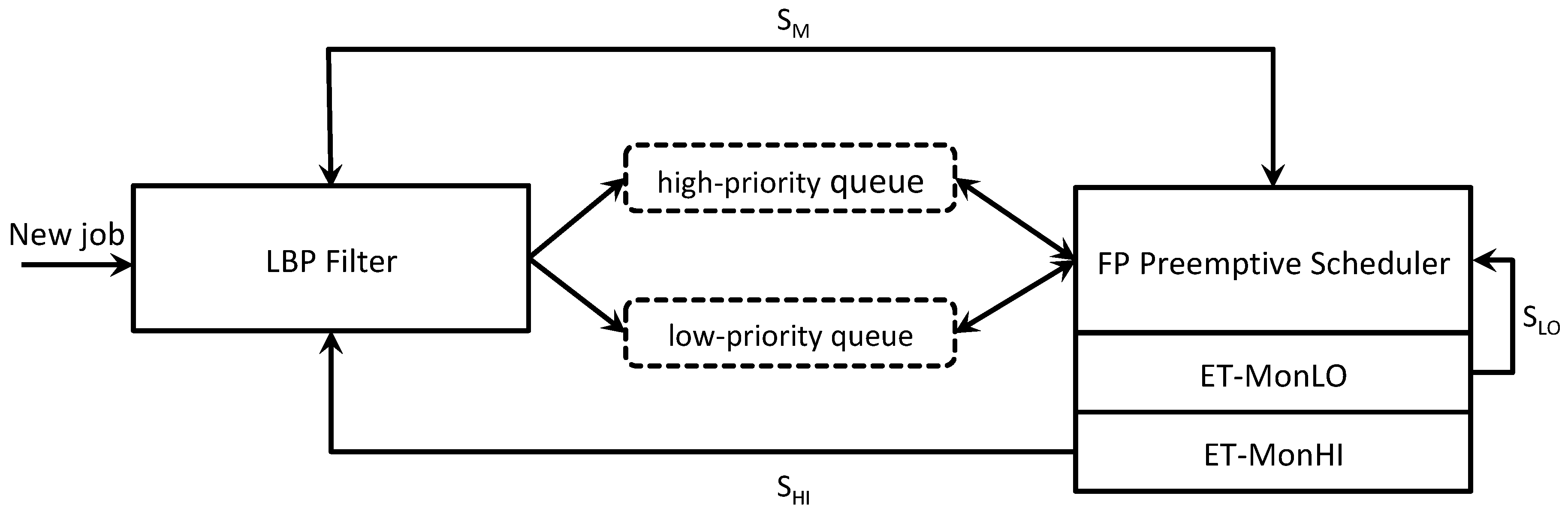
Figure 1 shows the components of LBP. The LBP filter is responsible for changing the execution modes. The system has two ready queues for jobs: the
high-priority queue represents the BP ready jobs queue while the
low-priority queue keeps the LO jobs that have been released during Bailout or Recovery modes or that have exceeded their
. Note that LO jobs inserted into the low-priority queue run until their deadline and
only when the high-priority queue is idle. Thus, such jobs cannot lead to any deadlines being missed. There are two job monitors to check, respectively, LO and HI jobs that overrun their
.
signals to the real-time scheduler the LO jobs that have to be inserted within the low-priority queue while
communicates to the LBP filter when a HI job exceeds its optimistic WCET to switch the execution mode to Bailout.
Similar to BP, LBP inherits from AMC the system execution behaviour, i.e., the system starts in a low-criticality execution mode and whenever a HI job exceeds its optimistic WCET, the system switches to a high-criticality execution mode where any LO job execution is prevented. Finally, the system goes back the starting execution mode in case of idle instant. Furthermore, LBP inherits from BP the control mechanism that is in charge of the execution mode changes that permits a fast recovery from the Bailout/Recovery modes back to the Normal mode. Such mechanism is based not only on the detection of a idle instant but also on the value of a decision variable named
Bailout Fund (BF). It is worth noting that LBP, as well as AMC and BP, implement dispatching policies that are independent and separated from the priority assignment used. Moreover, since a fixed-priority scheduler is used, no priority change is allowed.
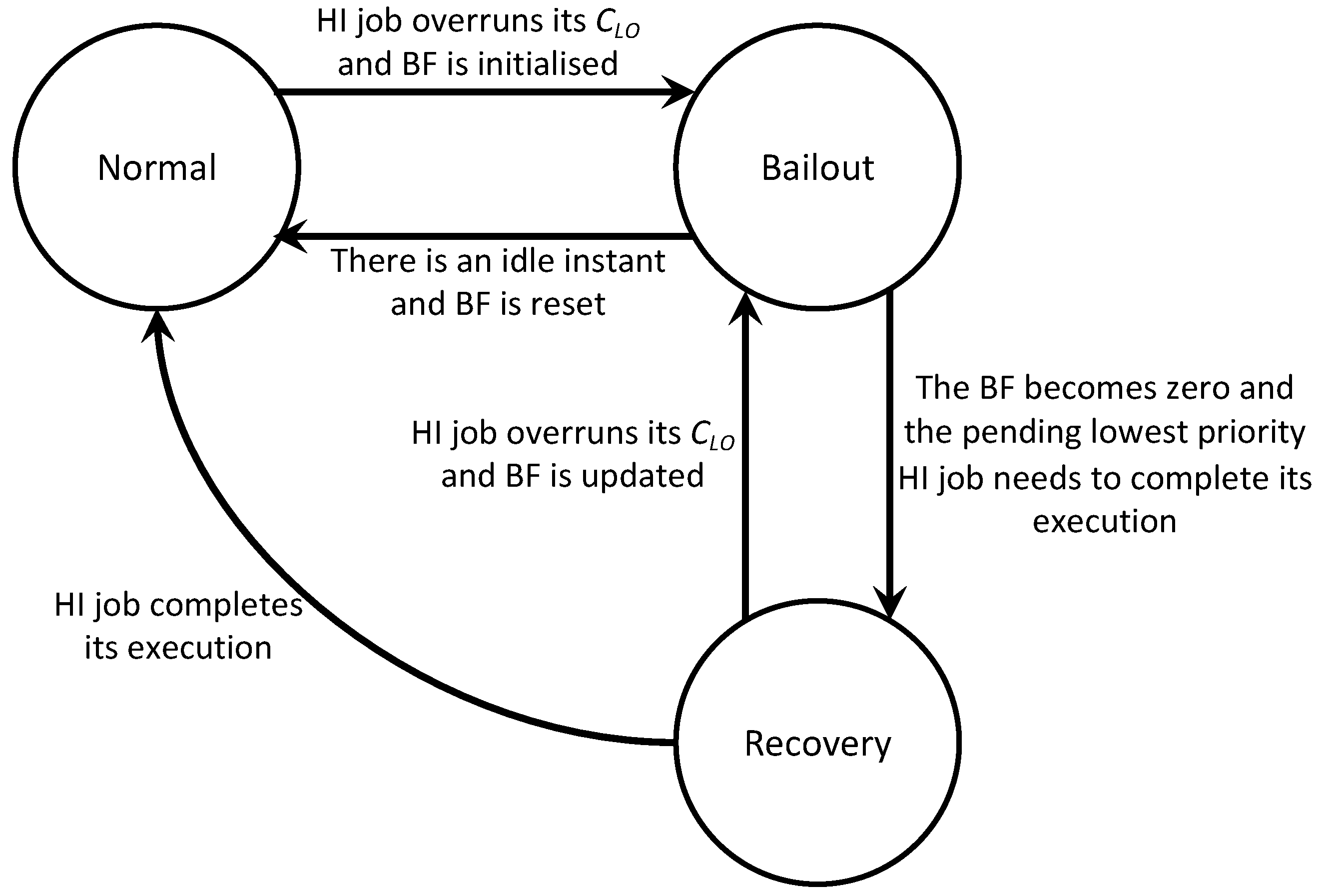
Figure 2 shows how the execution mode changes in the scheduling protocol. It contains the events that trigger the switch to a different execution mode together with the related update of the BF value. The system starts in Normal mode and then, if any HI job overruns its
, the BF variable is initialised and there is a change to Bailout mode. Once the system is in this mode, the BF variable is updated with the earlier completion of jobs, the release of new LO jobs or the HI jobs overrunning their
. If an idle instant occurs, then Normal mode is entered, whereas, if the BF becomes zero, then Recovery mode is entered. After the pending lowest priority HI job completes its execution in Recovery mode, the system goes back to Normal mode.
The difference between LBP and BP is that LO jobs released in Bailout and Recovery modes or exceeding their are inserted into the low-priority queue instead of being abandoned. This allows increasing the amount of LO jobs scheduled without interfering with the execution of jobs in the high-priority queue. In fact, LO jobs in the low-priority queue run until their deadline when the high-priority queue is idle. The essential difference in scheduling behaviour is that, in those cases where BP would be idle, LBP might have some tasks preserved in the low-priority queue that can now successfully be executed.
Whenever a job in the low-priority queue misses its deadline, it is removed. LO jobs released in Normal mode can continue to execute in both Bailout and Recovery modes and they could even overrun their deadlines as long as they do not exceed their . Below, is a detailed description of LBP in each of its execution modes:
Normal mode:
While all HI jobs execute for no more than their values, the system remains in this mode.
If any HI job overruns its without signalling completion, then the system switches into the Bailout mode and the BF is initialised to .
LO jobs that overrun their are interrupted and inserted into the low-priority queue.
LO jobs that have been inserted into the low-priority queue are executed during idle instants. If they do not complete within their deadlines, then they are removed from the low-priority queue.
Bailout mode:
If any HI job executes for its without signalling completion, then the bailout fund is updated by its maximum extra time budget: .
If any HI job completes with an execution time e, with , then its time left is donated to the bailout fund: .
LO jobs released in Normal mode that complete with an execution time of e, with , donate their time left to the bailout fund: .
If any HI job that already exceeded its completes with an execution time of e, with , then it donates its extra time left, reducing the bailout fund: .
LO jobs released in Bailout mode are not started but inserted in the low-priority queue to be executed during idle instants in Normal mode. Furthermore, when the scheduler would otherwise have dispatched such a job, the job’s budget of is donated to the bailout fund: .
If the BF becomes zero, then the lowest priority HI job that did not complete its execution (let this job be ) is recorded and the Recovery mode is entered.
If an idle instant occurs, then a transition is made to Normal mode, and BF is reset to zero.
Recovery mode:
LO jobs released in this mode are not started but inserted within the low-priority queue to be executed during idle instants in Normal mode.
If any HI job executes for its value without signalling completion, then the system switches back to Bailout mode and BF is initialised: .
When the job noted at the point when Recovery mode was last entered completes, then the system switches to Normal mode.
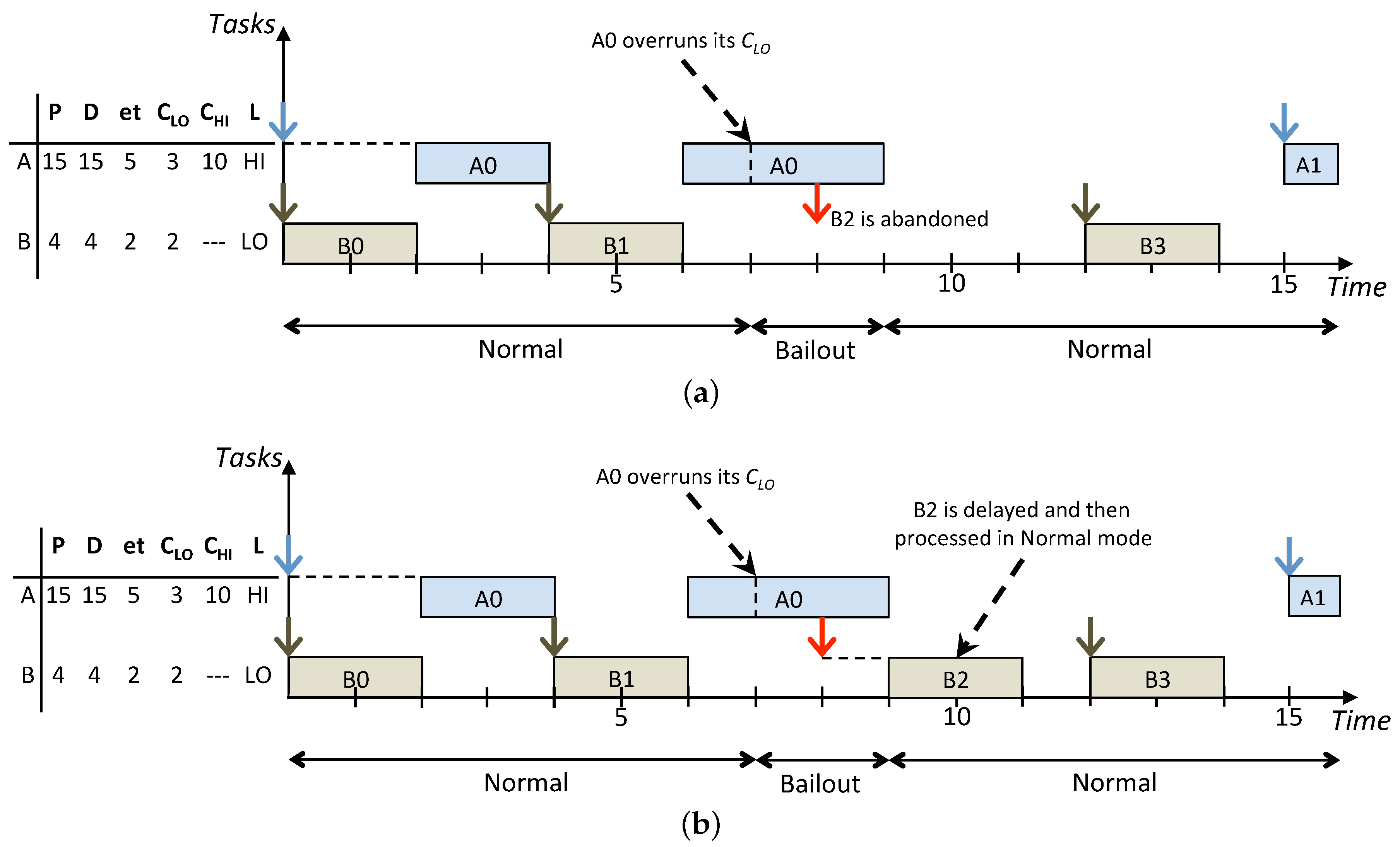
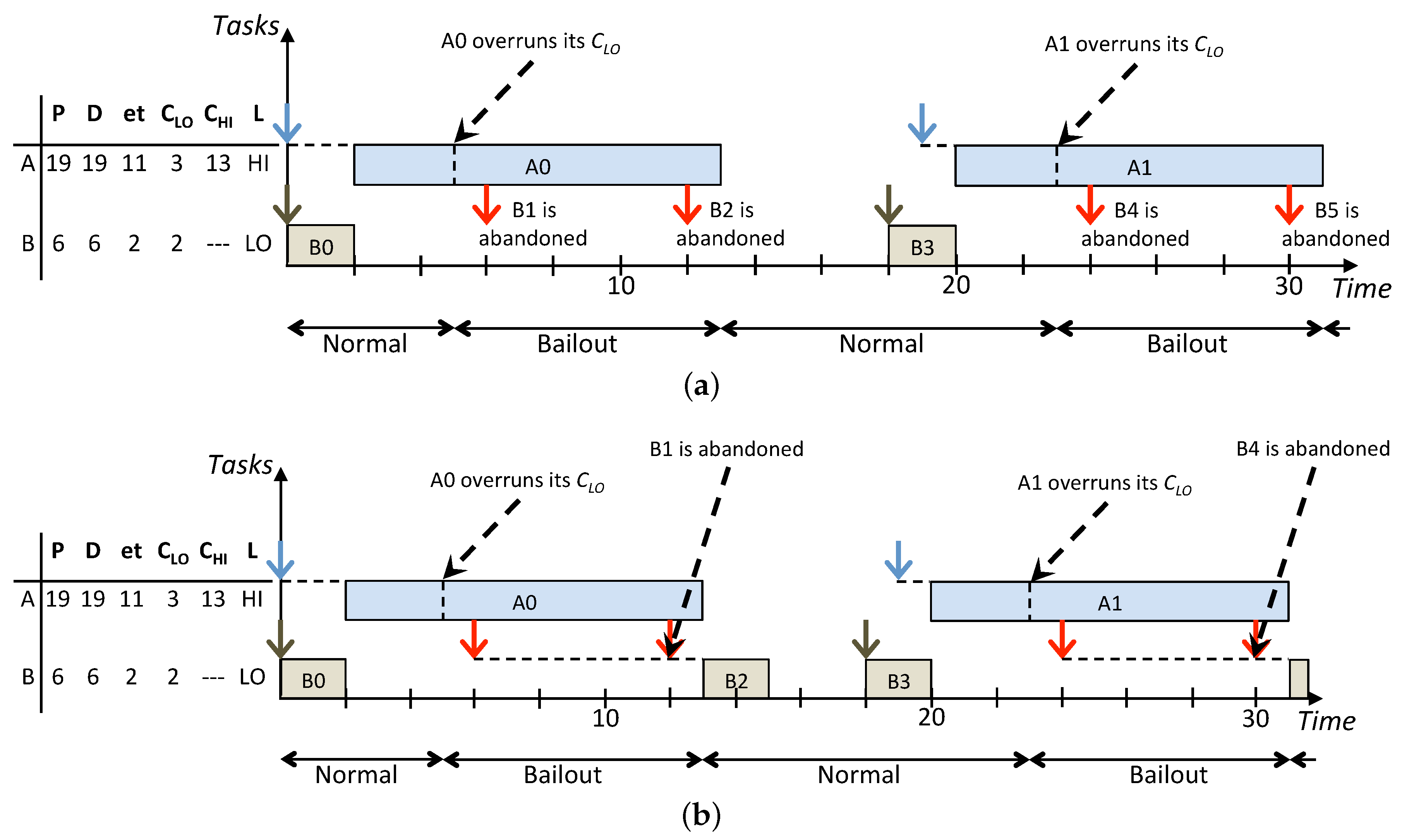
Figure 3 shows how the same task set is scheduled according to the On the one hand, the standard BP abandons all the LO jobs released during the HI criticality execution modes while the lazy approach allows to recover and schedule more LO jobs. In particular, in
Figure 3b, jobs
and
are released, respectively, at times
and
and they have the highest priority. Such jobs are inserted in the low-priority queue to be removed, respectively, at times
and
when they miss their deadlines and the next instance of the same task arrives. Furthermore, the LO jobs
and
released respectively at times
and
are executed afterwards in Normal mode since there are idle instants to exploit before their deadlines. Such example highlights how LO jobs that are delayed, instead of being abandoned, are executed during idle instants in Normal mode to not influence the real-time behaviour of jobs in the high-priority queue. Overall, compared with LBP, the standard BP results in a decrease of the system utilisation because, whenever there is interference among HI and LO jobs released in Bailout or Recovery modes, LO jobs are simply abandoned. On the other hand, LBP increases the processor utilisation by exploiting the system idle time and, by doing this, it improves the overall service provided to LO tasks, which is achieved by increasing the number of LO jobs that are processed.
6. Experimental Evaluation
In this section, we describe how we conducted our experiments and what were the final outcomes. We start by explaining how the experiments were structured.
Section 6.2 explains how task sets were created, what were our application scenarios and what scheduling methods we compared. Next,
Section 6.3 describes what type of performance metrics we considered to evaluate and compare different mixed-criticality scheduling methods. Finally,
Section 6.4 contains the description and discussion of results according to what is shown within tables and charts.
6.1. Task Set Generation
The aim of the task set generation was to simulate situations in which the system easily switches to the Bailout execution mode in order to show the effectiveness of the LBP methods over BP and its derivatives in systems with high load (using a utilisation factor of 0.6 or more). The system load computed according to the pessimistic WCET of all HI tasks within each task set was always greater than that computed according to the optimistic WCET of all its tasks. Furthermore, the execution times of HI tasks almost always exceeded their in order to trigger the mode change.
As a result, task sets were generated to have an overall utilisation factor that varied randomly between 0.60% and 0.75% with respect to the optimistic WCET of all tasks while the utilisation factor computed according to the HI tasks was always 0.75%. The number of tasks per task set varied randomly between 4 and 20. Within each task set, the amount of HI tasks varied randomly between 20% and 70% of the task set. Moreover, the execution times of HI tasks varied between the 90% of their and their , while the execution times of LO tasks was between 40% of their and 10% more than the . Priorities were assigned to tasks according to the Deadline Monotonic (DM) strategy: task instances with shorter deadlines had higher priorities.
6.2. Description of Experiments
We conducted different experiments, each consisting of a group of 3000 task sets randomly generated. Tasks within every task set have implicit deadlines and their periods varied randomly between 3 and 22. Every task set group belonged to one of the three scenarios specified below:
- HC-LP
contains job sets where all HI jobs have larger deadlines than all LO jobs. More precisely, LO tasks’ periods varied randomly between 3 and 10, while HI tasks’ periods varied between 14 and 22. Therefore, all HI jobs had lower priority than all LO jobs:
- HC-MP
contains job sets where HI jobs have deadlines that are smaller or larger than those of LO ones. In fact, periods of tasks, either HI or LO, varied randomly between 3 and 22. Therefore, HI and LO jobs had mixed priorities:
- HC-HP
contains job sets where all HI jobs have smaller deadlines than all LO ones. More precisely, HI tasks’ periods varied randomly between 3 and 10 while LO tasks’ periods varied between 14 and 22. This implies that all HI jobs have higher priority than LO jobs:
We compared the following scheduling protocols:
The standard Fixed-Priority Preemptive Scheduling with DM as priority assignment (FPPS-DM).
The standard Bailout Protocol (BP).
The Bailout Protocol with Gain Time (BPG), where each job that finishes before its optimistic time threshold in Normal mode gives its gain time to increase the time budget of next job ready to be scheduled.
The
Bailout Protocol-Slack (BPS) and the
Bailout Protocol-Slack and Gain Time (BPSG) that represent the execution of BP and BPG on task sets in which the
of HI tasks is appropriately increased via sensitivity analysis [
30,
31] while the schedulability is guaranteed according to AMC-rtb [
15].
The Lazy Bailout Protocol (LBP).
The Lazy Bailout Protocol with Gain Time (LBPG), the Lazy Bailout Protocol-Slack (LBPS) and the Lazy Bailout Protocol-Slack and Gain Time (LBPSG) that represent extensions of LBP made by using the offline scaling of of HI tasks with sensitivity analysis and the gain time collection at runtime.
We finally show the benefit of the lazy bailout approaches with respect to the former methods.
It is important to note that, if HI tasks all have higher priority than LO ones, then the scheduling problem so created becomes equivalent to the standard real-time scheduling problem since there is no criticality inversion. The same applies to those cases in which higher priority is assigned to the highest criticality tasks regardless of their periods or deadline as in
Criticality As Priority Assignment (CAPA) [
32].
Results of experiments are collected in
Table 1 and
Table 2, which refer to the different scenarios described above. For each scenario, we show the results with different scheduling protocols.
6.3. Description of Performance Metrics
This subsection introduces the criteria we used to assess performances of scheduling protocols that process dual-criticality task sets. To evaluate the results, we defined two types of performance parameters, i.e., task set schedulability that is relative to the whole amount of task sets and the global job set schedulability that is relative to jobs within each individual task set.
We conducted our experiments on three sets of 3000 task sets
, one per scenario (HC-LP, HC-MP and HC-HP). The task set schedulability formula
is defined as follows:
where
S could be either a simple task set
or set of task sets
and the category
represents the type of tasks within a set that is HI to indicate HI tasks, LO to indicate LO tasks and either when we use HI+LO. The function
depends on the scheduling protocol that is actually used and returns as output the set of task sets
in which there are no jobs missed of category
. The absolute values within the formula give the set cardinality. Equation (
4) allows deriving the percentages of tasks set in
that are successfully processed according to the category
as follows:
is the amount of task sets scheduled with no jobs missing their deadlines.
is the amount of task sets scheduled with no HI jobs missing their deadlines.
is the amount of task sets scheduled with no LO jobs missing their deadlines.
The task set schedulability permits showing the percentage of task sets in which no job of category misses its deadline. However, whenever a task set contains some jobs, either HI or LO, that miss their deadline, it is also useful to assess the level of service provided in terms of jobs completed within their deadlines and jobs abandoned or aborted. The job set completion rate method returns the percentage of jobs of category generated by a specific task set that complete within their deadlines.
The job set schedulability
is formally written as below:
The formula of the global job set schedulability
returns the average amount of jobs of category
processed within their deadline that has been generated by a set of task sets
:
As in the previous case, it is possible to filter the jobs meeting their deadline according to the category as below:
is the average number of jobs (either HI or LO) that is scheduled within a task set.
is the average number of HI jobs that is scheduled within a tasks set.
is the average number of LO jobs that is scheduled within a task set.
Table 1 and
Table 2 contain, respectively, the results about task set and global job set schedulabilities. It is possible to comment on the data according to scenario or scheduling protocol. However, we use figures to describe graphically what is contained within the tables and to allow an easier and quicker comparison among the results.
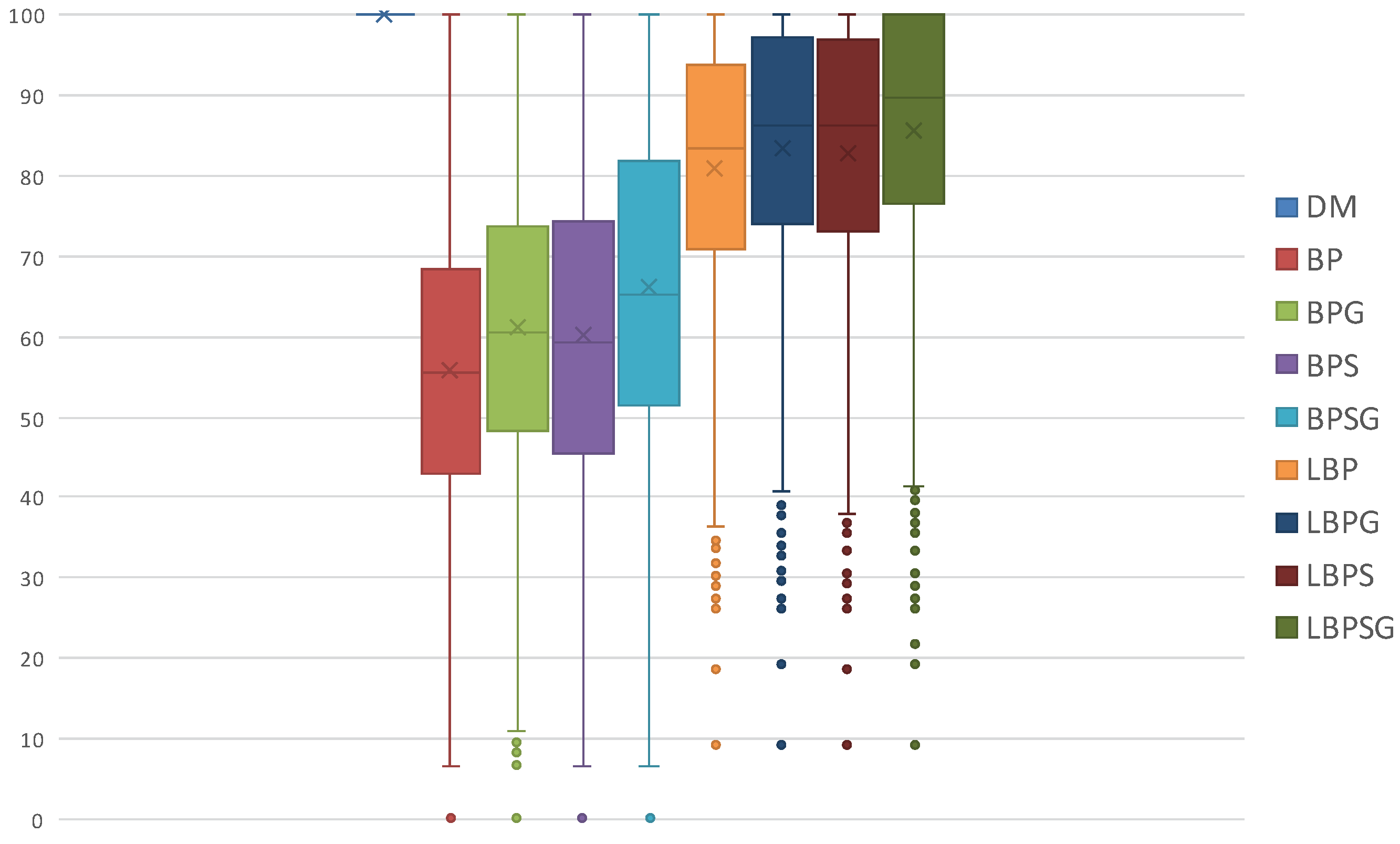
Task set and global job set schedulabilities are averages and do not give information about how data are distributed and about outliers. Therefore, we use also boxplots charts to show the distribution of LO jobs scheduled per task set. The information shown in
Table 1 is contained in
Figure 7a,
Figure 8a and
Figure 9a. On the other hand,
Figure 7b,
Figure 8b and
Figure 9b displays the average percentages of LO jobs completed within their deadlines.
6.4. Discussion of Results
This subsection is dedicated to study the outcome of the experiments. It contains figures that summarise the results of our experiments with dual-criticality job sets.
Figure 7 and
Figure 8 summarise the results in cases where there is criticality inversion. In these situations, if no HI job completes within its optimistic threshold estimate
, then very likely there will be some new incoming higher priority LO jobs that will interfere with it. Then,
Figure 9 contains information about cases in which all HI jobs have higher priority than LO jobs since all the critical jobs have smaller deadlines. This basically leads to having no interference between HI and LO jobs and thus no criticality inversion occurrence during the scheduling process.
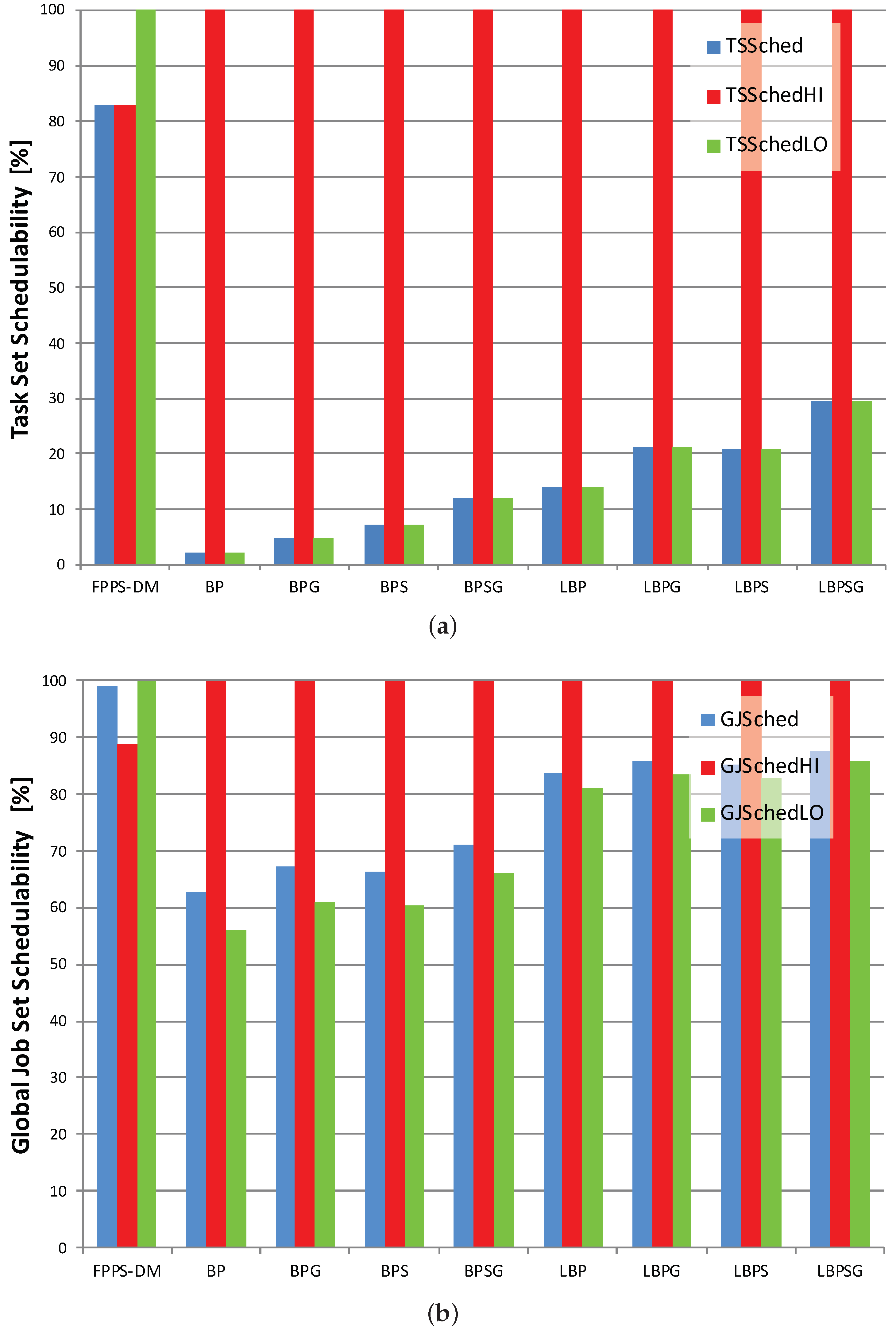
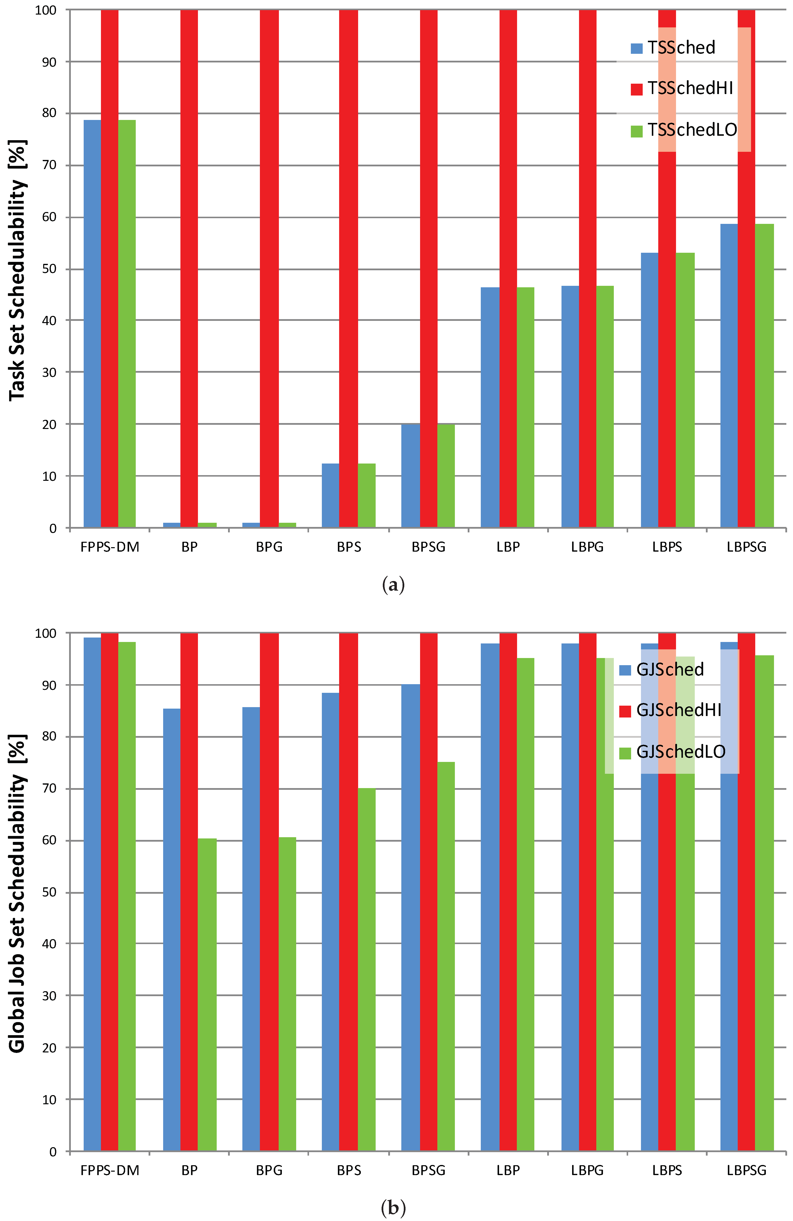
Looking both at task set and job set schedulabilities results in
Figure 7,
Figure 8 and
Figure 9, it is possible to notice that, compared with mixed-criticality methods, the standard deadline monotonic approach always schedules jobs only according to priorities. In this case, the percentages of HI and LO jobs successfully scheduled mainly depend only on their priority, with all LO jobs always meeting their deadlines in HC-LP scenario and all HI jobs always meeting their deadlines in HC-HP scenario. Conversely, the mixed-criticality protocols always assure that there are no HI job missed regardless of job priorities. The experiments confirm what is stated in
Section 5 with LBP in which the percentage of task set scheduled with no jobs missed is between 13% and 46% while BP schedules no more than 2.20% of task sets with no jobs missed.
Then, where the offline and online complementary techniques are used, there is an increase in LO jobs successfully processed. Furthermore, the usage of sensitivity analysis and the gain time mechanism have the same effects when applied both to the standard or to the lazy bailout method. A noticeable result is that each LBP-based approach always increases the amount of LO jobs completed within their deadlines compared with the corresponding standard BP-based protocol. Overall, according to the criteria defined in
Section 5, LBPSG is the protocol that outperforms all other mixed-criticality scheduling methods with an amount of task set scheduled with no jobs missed that is between 29.57% and 58.57%.
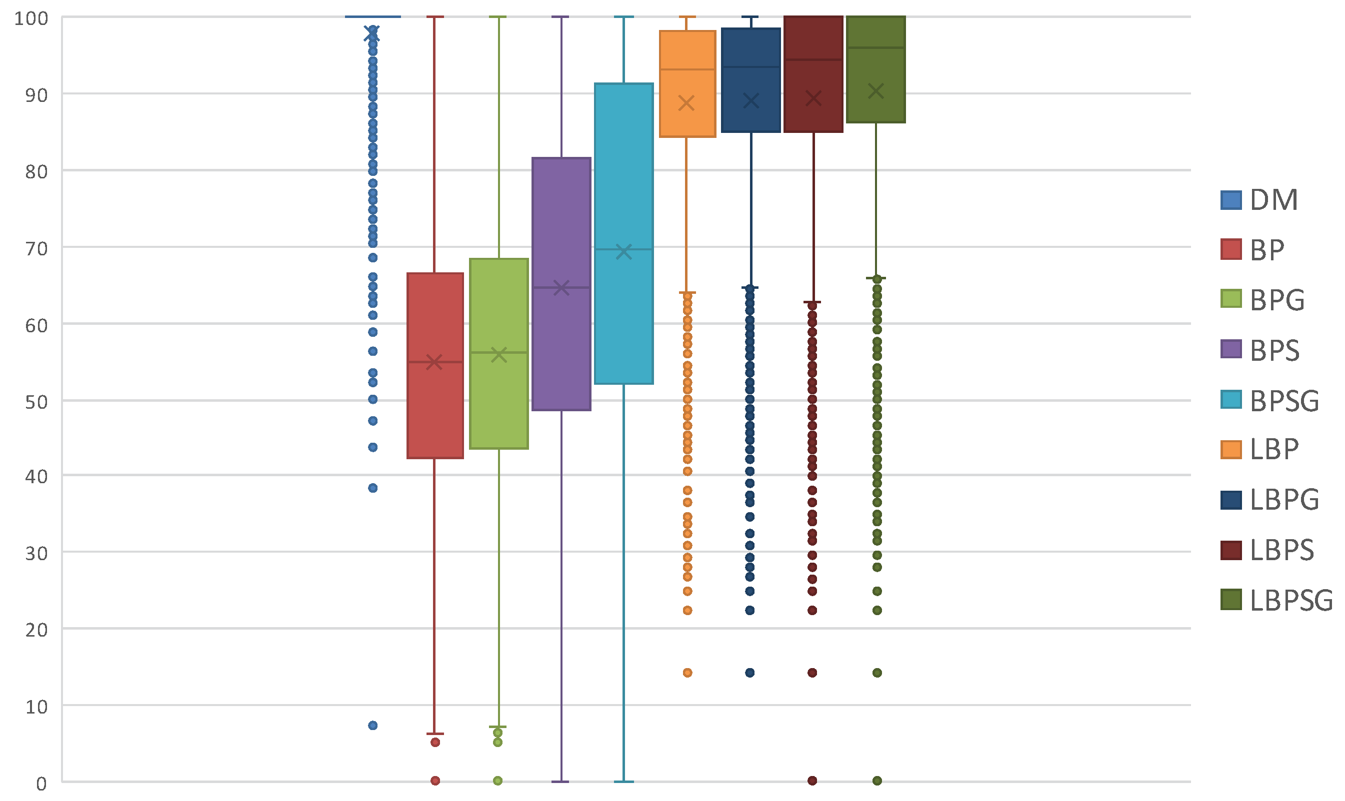
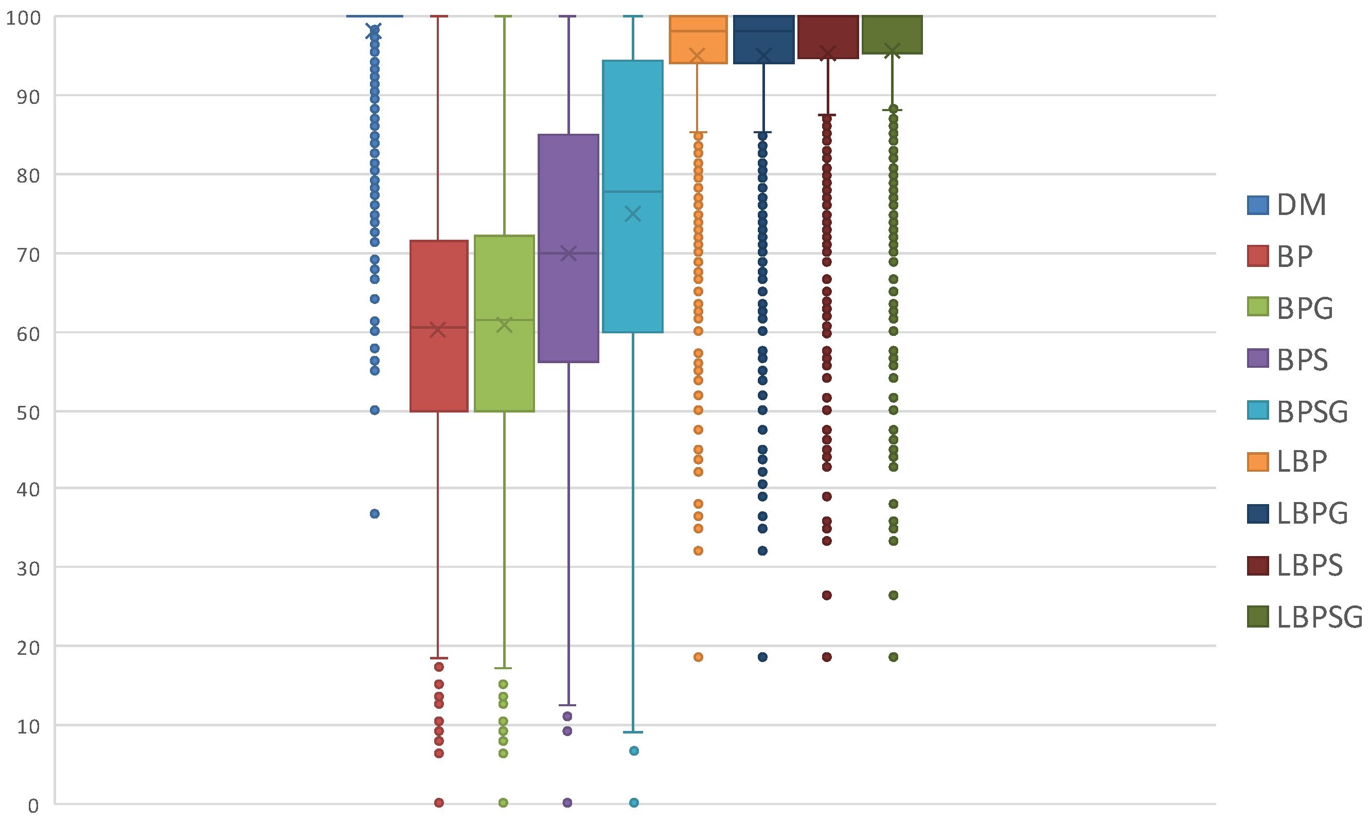
Figure 10,
Figure 11 and
Figure 12 display the distribution of the LO jobs percentages per task set that are completed within their deadlines. Each scheduling protocol is represented by a box-and-whisker diagram with the box itself representing the range in which at least 50% of results tend to be concentrated. The box also contains the indication of the median and the mathematical average of all the LO jobs scheduled by the related protocol. The results highlight how the LBP-based methods always increase the LO jobs success rate, as defined in
Section 5, compared with the former BP ones.
In conclusion, the experiments confirm what is stated in
Section 5 with lazy approaches increasing the amount of LO jobs successfully scheduled while guaranteeing the correct completion of all HI jobs. In other words, LBP has better mixed-criticality performances than BP, while LBPS, LBPG and LBPSG have, respectively, better mixed-criticality performances than BPS, BPG and BPSG. Finally, the usage of mixed-criticality protocols is recommended in HP-LP and HC-MP scenarios, i.e., when HI jobs could have lower priorities than LO jobs.
7. Summary and Conclusions
Mixed-criticality scheduling is important for cyber-physical systems to provide robustness against resource shortage. In this paper, we have introduced the mixed-criticality scheduling protocol
Lazy Bailout Protocol (LBP). LBP is a scheduling protocol for uni-processor platforms and is a refinement of Bailout Protocol (BP). We have also introduced a formal criterion to compare performances among mixed-criticality scheduling protocols. This criterion prioritises HI jobs against LO jobs, where HI indicates high-criticality and LO stands for low-criticality. Based on that criterion, we have proven that the complementary techniques used in [
11] always contribute to increase the performances of the scheduling protocol. Similar to BP, LBP and its derivatives always guarantee the correct completion of HI jobs. Moreover, we have shown that LBP always schedules more LO jobs than BP and that each LBP derivative always outperforms the corresponding BP-based approach.
Besides these formal results, we have also presented experiments that give quantitative values of the comparisons between the different mixed-criticality scheduling protocols. LBP schedules between 13.93% and 46.63% of task sets with no jobs missed while BP at maximum schedules no more than 2.20% of task sets with no jobs missed. Finally, the experiments confirm that LBP is equivalent to BP in guaranteeing HI jobs and that the derivatives of LBP (LBPS, LBPG and LBPSG) outperform all the equivalent BP-based protocols by increasing the amount of LO jobs successfully scheduled. Overall, LBPSG has shown the best mixed-criticality performance with an amount of task sets processed with no jobs missed that is between 29.57% and 58.57%.
Future work will be on extending LBP towards support for many-core platforms.


