Article

Fault Classification of Axial and Radial Roller Bearings Using Transfer Learning through a Pretrained Convolutional Neural Network

1
Department of Engineering Sciences, University of Agder, 4877 Grimstad, Norway
2
NORCE Norwegian Research Centre AS, 4877 Grimstad, Norway
*
Author to whom correspondence should be addressed.
Designs 2018, 2(4), 56; https://doi.org/10.3390/designs2040056
Submission received: 23 November 2018 / Revised: 13 December 2018 / Accepted: 16 December 2018 / Published: 19 December 2018

Abstract

:
Detecting bearing faults is very important in preventing non-scheduled shutdowns, catastrophic failures, and production losses. Localized faults on bearings are normally detected based on characteristic frequencies associated with faults in time and frequency spectra. However, missing such characteristic frequency harmonics in a spectrum does not guarantee that a bearing is healthy, or noise might produce harmonics at characteristic frequencies in the healthy case. Further, some defects on roller bearings could not produce characteristic frequencies. To avoid misclassification, bearing defects can be detected via machine learning algorithms, namely convolutional neural network (CNN), support vector machine (SVM), and sparse autoencoder-based SVM (SAE-SVM). Within this framework, three fault classifiers based on CNN, SVM, and SAE-SVM utilizing transfer learning are proposed. Transfer of knowledge is achieved by extracting features from a CNN pretrained on data from the imageNet database to classify faults in roller bearings. The effectiveness of the proposed method is investigated based on vibration and acoustic emission signal datasets from roller bearings with artificial damage. Finally, the accuracy and robustness of the fault classifiers are evaluated at different amounts of noise and training data.

1. Introduction

Failure on rolling bearings is one of the most frequent system failures, resulting in huge losses of productivity in drivetrains installed in remote and harsh environment areas. Defects on bearings contribute to over 40% of faults in rotating machinery [1]. If a bearing fault is well predicted, the risk of long-term system breakdown can be prevented, and a replacement of the faulty bearing will be done at the right time. Faulty bearings can be detected by analyzing current, vibration, or acoustic emission signals. Current signature analysis can be useful to detect limited faults on bearings, which need to be connected to a shaft driven by an electric motor. Vibration analysis is preferred to monitor conditions of bearings in most mechanical systems, where accelerometers are usually installed in place. In critical applications, acoustic emission signals can be used to detect bearing faults at an early stage due to its higher sensitivity and convenient installation without being involved in the system.
Processing data and understanding faulty features in vibration and acoustic emission analysis need skilled manpower with advanced knowledge of bearing faults [2]. Vibration signals associated with faults typically originates from high-frequency resonance in the housing structure excited by low-frequency impacts related to the contact between a fault and other bearing components. The accelerometers installed on the bearing housing are very sensitive to any forces generated in a system. This makes collected signals from the accelerometers very complicated due to the interference of noise. The complexity of the output signals from the collected acoustic emission sensors can be even worse due to its higher sensitivity and is worse in highly disturbed environments.
To predict bearing faults based on the mentioned signals, common processing, i.e., fast Fourier transform (FFT), short-time Fourier transform (STFT), and continuous Wavelet transform (CWT) in [3], and wavelet transform (WT) with kurtosis [4], could be used to detect signals associated with the faults. Such a signal processing technique is useful to observe characteristic frequencies in time and frequency representations. However, missing a harmonic in a spectrum or the appearance of harmonics at characteristic frequencies due to noise might cause misclassification. Further, the effectiveness of this conventional approach strongly depends on manpower skill, training, and relevant experience.
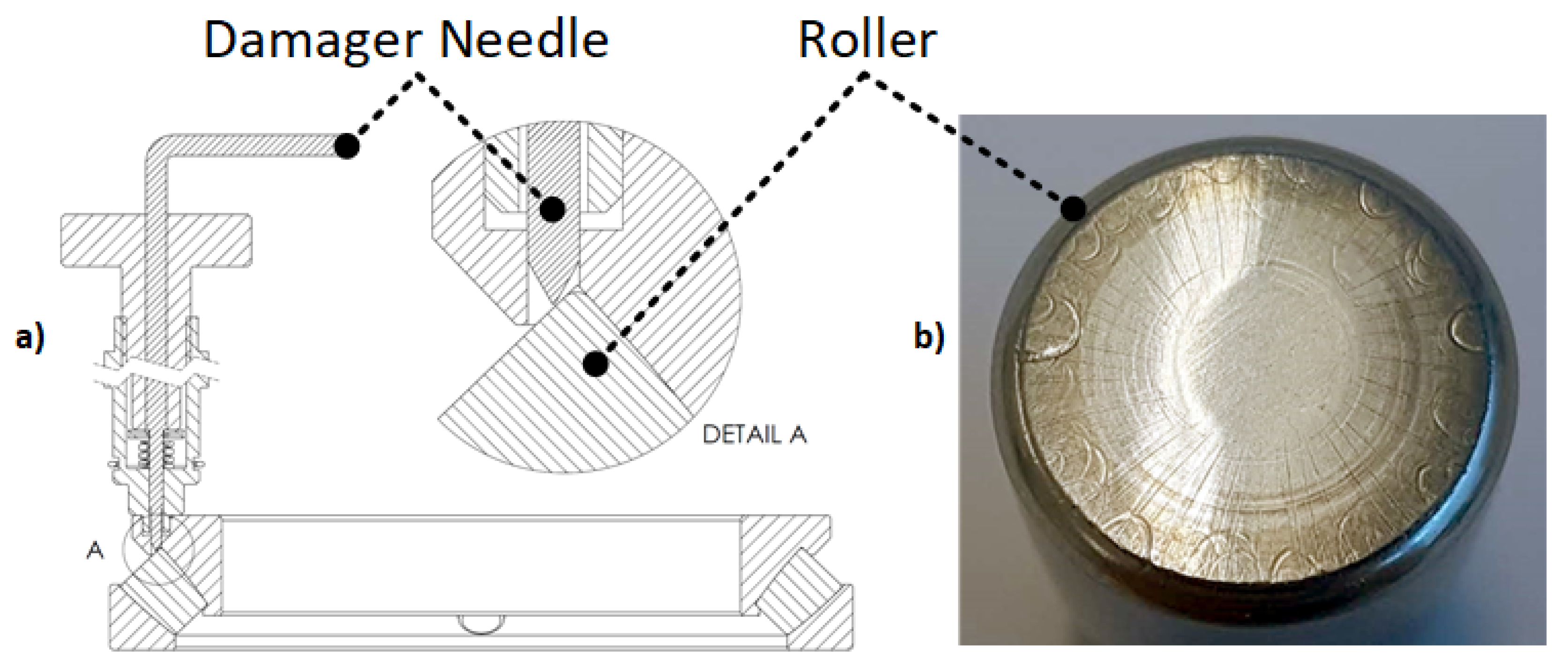
Unlike conventional bearing faults such as spalling on races or rolling elements, roller-end wear in axial roller bearings might not produce periodic harmonic components associated with faults. In a previous study by the authors [5], scratches on an axial bearing were observed on roller ends of a tapered axial roller bearing in an offshore drilling machine, but no particular bearing frequency was steadily detected in the spectrum. However, acoustic emission data showed an energy increase with higher damage severities. Detecting bearing defects without a characteristic frequency or predefined knowledge of the fault signature is a big challenge in fault diagnosis.
To address the mentioned challenges, an automatic system for fault detection and classification applicable to both vibration and acoustic emission signals can reduce the manpower dependence and time consumption for condition monitoring of the roller bearing in industry. As argued in [6], increasing the performance of the detection system might be more important than looking for highly reliable features. Model-based, data-driven, or hybrid algorithms are common in automatic fault diagnosis [7,8,9,10]. The model-based diagnosis needs both a detailed physical model of the system and its accurate parameters, which are very hard to obtain in reality. Without a physical model [11], the data-driven approach using statistical or machine learning algorithms is attractive for an automatic diagnosis system. To enhance the accuracy of fault detection, statistics methods should be based on the frequency spectrum to reduce false and missing alarms [12]. Alternatively, machine learning methods, namely support vector machine (SVM) [13,14], decision tree (DT) [15], and various neural network architectures [16,17] combined with advanced signal processing can be used to find the complex relations on the feature space by using predefined time-frequency features, being based on fault characteristic frequencies. However, without the characteristic frequencies, the mentioned methods have great difficulty in classifying bearing faults [18].
This work focuses on developing a simple automatic fault diagnosis method for roller bearings, requiring less human intervention or domain knowledge of features. Using transfer learning (TL) allows us to reduce the time and complexity of generating features for fault classification. Further, TL is very helpful for a bearing fault diagnosis if the available data for training and validation are limited in industry [16]. Within this work, a pretrained version of the well-known AlexNet convolutional neural network (CNN) architecture [19] is applied to CWT spectrograms of vibration and acoustic emission signals. Then, the CNN is either fine-tuned to perform classification directly or to extract features used to train and validate two classifiers using SVM and sparse autoencoder-based SVM (SAE-SVM). The robustness of the proposed method is tested at different signal-to-noise ratio (SNR) levels.
The remainder of the article is organized as follows. In Section 2, the proposed methods are detailed. In Section 3, the experimental setup and preprocessing are presented. In Section 4, the results of the fault detection and classification are presented. Further, the discussion of the presented results is detailed in Section 5. Finally, the paper is concluded in Section 6.

2. The Proposed Method

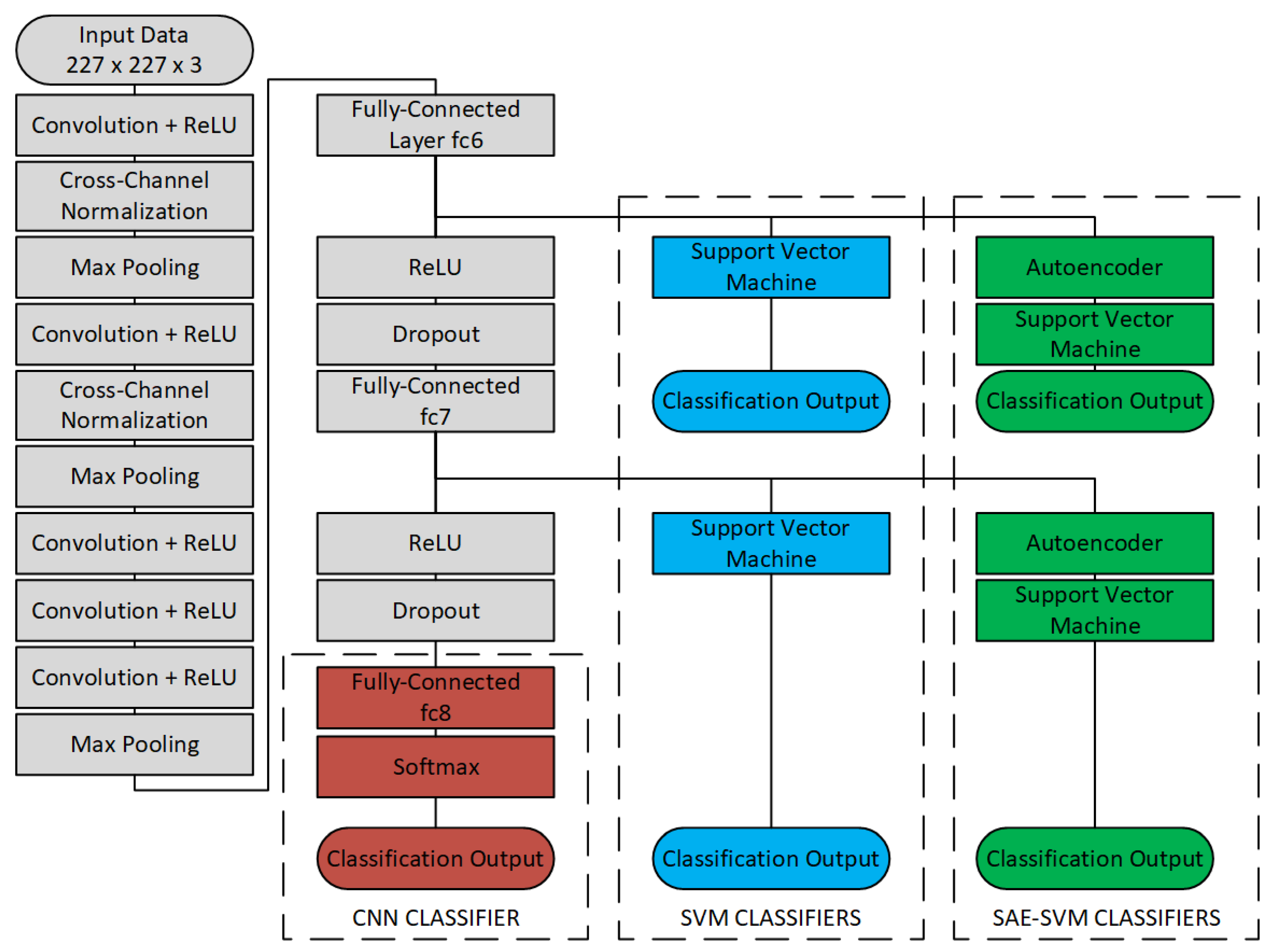
A diagram of the proposed fault classification is shown in Figure 1. The vibration signals need to be converted to images as pixels or a matrix (227 × 227 × 3, height by width by depth) before feeding them to the AlexNet architecture. Within this process, images or spectrograms of vibration signals are formed by three channels (red, green, and blue (RGB)), resulting in a depth of three. The spectrograms go though several convolutional layers, acting as learnable filters to detect the presence of specific features from the input, and produce matrices ( M × M × L ) with M < N and L-size filters. This work utilizes a pretrained version of the AlexNet architecture [19], obtained from the Berkeley Vision and Learning Center caffe repository on GitHub [
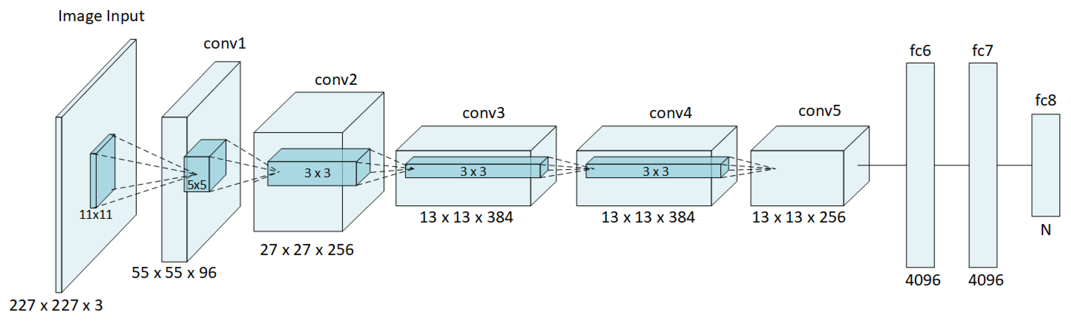
20], through the MATLAB Deep Learning Toolbox. AlexNet consists of five convolutional (conv1–conv5) and three fully-connected (fc6–fc8) layers, as illustrated in Figure 2, in which numbers outside the boxes illustrate the dimension in each layer and numbers inside the boxes indicate the filter sizes of the convolutions. The architecture uses rectified linear units (ReLU) as activation functions and dropout layers to prevent overfitting. Three classifiers will be described in this section: CNN, SVM, and SAE-SVM. For the two latter, features from the pretrained network will be extracted at both layer fc6 and fc7 and used to train two instances of the classifiers.

2.1. Convolutional Neural Network-Based Fault Classifiers or Retrained CNN

Given the performance of CNNs in image classification, they can be fully trained to classify patterns or spectrograms generated by CWT correctly [21]. However, training a network from scratch is very time consuming, requiring GPU programming, tuning of hyperparameters, etc. The first classifier uses transfer learning through fine-tuning of a pretrained CNN, e.g., the AlexNet architecture, to reduce the complexity of the training process. Instead of retraining the complete network from scratch, only the final classification layer is replaced, which maintains most of the already gathered information from the training on the imageNet database. To make sure most of the pretrained weights are maintained, the learning rate for the classification layer fc8 is increased to 20-times the overall learning rate. After replacing fc8 with a fully-connected layer of size 2 (equal to the number of classes), the network has approximately 60 million trainable parameters. Because of pre-training, fine-tuning the CNN to classify new data can then be done by using a smaller dataset of CWT spectrograms. This adaptation of a pretrained network is time-saving and very helpful for inexperienced users. Table 1 describes the parameter setting for the CNN-classifier.

2.2. Support Vector Machine-Based Fault Classifier

Support vector machines are supervised learning models for data classification. Given a set of training data of dimension K, the algorithm finds the hyperplane, a subset of the feature space of dimension K 1 , which provides the best separation between classes in the training data [14]. This is a quadratic optimization problem, which also removes the local minima being present in neural networks [22]. Each input image generates a set of features at each layer throughout the network. Instead of retraining the final classification layers like in Section 2.1, this classifier extracts the features directly at a higher level. This method is built on on the assumption that filters in the convolutional layers are trained to detect features that are also suited to discriminate features associated with the bearing faults.
The generated feature space from AlexNet has dimension N = 4096 for both layer fc6 and fc7. The objective of using data at fc6 or fc7 is to study whether the extra ReLU, dropout, and fully-connected layer from TL affects the accuracy of SVM classifications or not. By using the pretrained network to generate features, it is not necessary to design any features tailor-made to the application. Instead, the SVM is trained as set in Table 2.

2.3. Sparse Autoencoder Combined with SVM Classifier

The autoencoder is designed to replicate its input at its output in an unsupervised fashion, which can be used for both unsupervised feature extraction and image denoising [23]. An autoencoder is basically a single fully-connected layer of size P, referred to as the hidden layer, that is trained to reconstruct its input by minimizing error over the training dataset. Labels are not considered during training. One could assume that not all these features are equally important or necessary in order to perform classification. However, computational burden is a product of feature space dimension, N, and hidden layer size, P. By using the features from fc6 or fc7 instead of the input image, N is reduced from 154,587 to 4096, dramatically reducing the computational burden. Denoising AEs and sparse AEs are commonly used in literature. The denoising AEs are to partially corrupt input data and capture the original data removing noise, while the sparse AEs are to learn the features and structures within the input data. With a hidden layer size of P = 100 , the SAE is used in this paper with a sparsity proportion of 0.05 to identify features from fc6 or fc7. The identified individual features are classified by SVM as described in Section 2.2. Detailed settings of the SAE parameters are given in Table 3.

3. Experimental Setups and Datasets

The proposed method is evaluated using two separate datasets, consisting of time-waveform signals from two different bearing test rigs:
  • Dataset 1: Vibration data from the NU220 ECP radial bearing with seeded faults.
  • Dataset 2: Acoustic emission signals from an artificial roller end scratch generation from an in-house test setup for axial tapered roller bearings.
The two datasets represent the two different situations discussed in Section 1. Dataset 1 contains periodic transients at bearing fault frequencies, while Dataset 2 contains aperiodic bursts of acoustic energy from scratch formation on the roller end.

3.1. Dataset 1: Radial Roller Bearing Test Rig

The radial bearing tests were conducted using a radial bearing test rig at the Institute for Machine Elements and Systems Engineering at RWTH Aachen University. A triaxial accelerometer was mounted on the bearing housing, giving two radial channels and one axial channel. The location is shown in Figure 3. For this paper, the two radial channels were used in the analysis.
The test bearing, a radial bearing of type NU 220 ECP, was tested with two different fault types. Fault Type 1 (FT1) is a severe outer race (OR) fault, while Fault Type 2 (FT2) is a smaller rolling element (RE) fault. Data were classified as either healthy (HE) or damaged with subcategories of OR and RE faults. However, each bearing only had one type of damage or a single fault under test; thus, detecting faults in each bearing is a binary classification problem. The seeded OR and RE damages in the bearing can be seen in Figure 4.
Impact energy is reduced as the load decreases, making fault detection more challenging. According to the recommendation of the bearing manufacturer, the minimum radial load for the test bearing is 2.09 kN at 1000 rpm. Data chosen for analysis were collected with a constant radial load of 5 kN to test the proposed method under the most difficult conditions while complying with the bearing operating specification. The test operating conditions are described in Table 4, from which 560 CWT spectrograms were produced: 25% belonged to the damaged case, while 75% were in the healthy case. Twenty five percent of the dataset was reserved for validation of the algorithms, and the remaining 75% was used for training. Further, as shown in Table 5, the proposed algorithms were also trained with 25% and 50% data.

3.2. Dataset 2: Axial Roller Bearing Test Rig

The axial bearing test rig was designed and built at the University of Agder. A schematic drawing and picture of the test setup are shown in Figure 5. This testbed was built based on an observations from an offshore drilling machine. It was found that wear occurred in the rib-roller area of a large, tapered rolling element bearing with a characteristic arc-shape. The developed test rig was to investigate the fault signature of such scratches occurring during operation. A spherical tapered rolling element bearing was placed inside an enclosed test unit containing a lubricant. The bearing was loaded using a hydraulic cylinder and rotated using a direct-drive permanent magnet synchronous motor. A damage mechanism allowed the roller to be scratched during operation.
The rib-roller contact area is prone to wear due to the relative sliding motion. Consider a simplified example where a particle large enough to break the oil film is stuck between the rib and roller end, stationary with respect to the rib. It can be shown that the trace of the particle on the roller will resemble a segment of an epitrochoid as the roller passes, which complies with the observations from the offshore drilling machine. This type of damage differs from localized damages such as spalling. In the experiments on the axial bearing test rig, we were able to replicate this damage using a hardened needle, as shown in Figure 6. To detect faults on the rolling element bearing, one channel of acoustic emission data, shown in Figure 5, was used to collect time-series data (Dataset 2) for analysis.
Dataset 2 contains two labels: healthy (HE) and scratch (SC). A total of 600 images were generated, of which 200 were from the damaged class. Again, 25% of the data was reserved for validation and the rest used for training. Table 6 shows the number of images used for training and validation in the different cases. This dataset was collected at a very low speed of 1 rpm, as the current test setup did not allow consistent scratching at higher rotational speeds due to possible breakage of the needle. Axial load was kept constant at 50 kN during the tests.

3.3. Preprocessing

Collected vibration data are in time domain. If supplying the time domain signal directly to the CNN, the CNN pattern recognition is constrained by the 1-dimensional convolution [24]. To detect signals associated with faults in both the time and frequency domains, input data of the CNN should be converted to 2D spectrograms with 2D convolution. The AlexNet architecture deals with the 2D convolution, being fed with 227 × 227 × 3 RGB images. Continuous wavelet transform (CWT) is used in the preprocessing to convert the collected vibration signals to time-frequency representations or spectrograms. Short-time Fourier transform (STFT) can be an alternative method, but requires an extra parameter. Selecting the best method to produce proper spectrograms is out of scope of this work. CWT is applied to both Datasets 1 and 2 in the following sections. To study the effect of training data on the performance of the proposed fault classifiers, namely CNN, SVM, and SAE-SVM, the training data were reduced by steps of 25% from 75%–25% while keeping the same amount of validation data of 25%, as shown in Table 5 and Table 6. Analysis results on the datasets, from two different test setups of radial and one axial bearings will be described in more detail in Section 3.1 and Section 3.2 below.
The data in Dataset 1 were collected in the time domain under different operating conditions, with the speed ranging from 100 rpm–1000 rpm. Normalization of root mean square (RMS) was performed to make time series more comparable. To increase the amount of training data, each time series was split into segments of two revolutions. This transforms the signal from the time domain to the order domain. The number of samples per revolution f o r d e r was calculated as the sample frequency f s a m p l e divided by the shaft frequency f s h a f t , as written in Equation (1). To test the robustness of the proposed method against noise, white Gaussian noise (WGN) was added to the time-waveforms in Dataset 1. The raw signal (SNR1) was considered as a reference for WGN power at other SNR levels.
f o r d e r = f s a m p l e f s h a f t
The number of samples in each segment N s e g was then calculated as in Equation (2), where n r e v is the number of revolutions to be included in the segment. n r e v = 2 was used in this work. The modification of the time scale for each segment is effectively a transformation to the order domain, which allows the spacing between transients to be kept constant at different speeds. Figure 7 shows the difference in time and time-frequency representations between two speeds of 100 and 1000 rpm in the case of the outer-race fault in Test Setup 1. While the transient peaks were more or less equally spaced, they showed up as lines at 100 rpm, but more like “blobs” at 1000 rpm.
N s e g = n r e v · f o r d e r
Noise was added to original vibration signals of Dataset 1 to test the robustness of fault classifiers based on CNN, SVM, and SAE-SVM. Table 7 summarizes the SNR levels added to the vibration signals. Figure 8 shows the exemplary original and vibration signals under different SNRs specified by 0, −3 and −10 dB. Impacts due to outer race defects could be easily observed in the original signals (top figure). Increasing noise to the signal causes the fault impacts to be mixed with the noise, resulting in a big challenge of fault detection if using signal processing techniques alone. Figure 9 shows a detailed flowchart of preprocessing for Dataset 1 with an outer race defect on the axial roller bearing. After the rms normalization, the original signal and signal under noise were subdivided into segments of two revolutions, which were converted to spectrograms by using CWT.
Dataset 2 consists of 10-s acoustic emission waveforms, which were recorded at a sampling frequency f s a m p l e = 1 MHz. Unlike Dataset 1, no noise was added to the acoustic emission data. Bursts collected in acoustic emission data occurred with inconsistent amplitudes throughout time; thus, adding white noise would cause a large share of the bursts to be undetectable. Order normalization is also not necessary, as all data were collected at the same low speed. Each 10-s of data was then subdivided into segments of 1 s, which were converted to spectrograms by CWT. Figure 10 shows the process of converting time series data to spectrograms in the case of scratches in the bearing, in which Segment 3 (2–3 s) and Segment 9 (8–9 s) are shown as exemplary spectrograms. Weak vertical lines are visible, corresponding to bursts of acoustic emission energy.

4. Results of Roller Bearing Fault Classifications

This section first presents the results of preprocessing, converting time-series signals to images or spectrograms for CNN algorithm. Further, the process of including noise in the original vibration signals is described. The fault classification results from the radial bearing test rig are presented in Section 4.1 and the fault diagnosis or scratch detection in the axial tapered bearing in Section 4.2.

4.1. Fault Classification for the Radial Bearing Based on Vibration Signals

In this section, the performance of classifiers, namely CNN, SVM, and SAE-SVM, is evaluated based on their accuracy of classifying faults in a radial bearing. Features fc6 and fc7 generated from AlexNet using Dataset 1 were fed into three fault classifiers. The dataset included two fault types (FT): outer race (OR) and rolling element (RE). Four SNR levels were investigated in each fault type, in which SNR1 was without noise, while other SNRs are shown in Table 7. The classification results at 75%, 50%, and 25% training data are summarized in Table 8. The CNN classifier was a fine-tuned version of the pretrained network, while the SVM and SEA-SVM classifiers were implemented on both fc6 and fc7 features, as mentioned in Figure 1, resulting in CNN, SVM fc6, SVM fc7, SAE-SVM fc6, and SAE-SVM fc7 in Table 8.
We can see from Table 8 that the overall trend is that the accuracy dropped with the decrease in SNR and the reduction in training data. As shown in the confusion matrices in Figure 11, the misclassification was not consistent. Healthy (HE) was considered as a negative class, while damaged was considered as a positive class. Target class refers to the ground truth, while output class was the classifier output. At low noise levels, the algorithms tended to give more false alarms than missed detections. For Fault Type 2, RE damage, this pattern changed between SNR3 and SNR4. The number of misclassifications increased more than false alarms.

4.2. Fault Classification for the Axial Roller Bearing Based on Acoustic Emission Signals

Validation accuracy for the axial data, shown in Table 9, was in general above 95%, except for SAE-SVM at fc7. These results are shown in more detail in Figure 12. The confusion matrices show that for 75 and 25% training data, the classifier was not able to separate classes and labeled all data as healthy. In the 50% case, all healthy data were misclassified as damaged. Additionally, some damaged cases were misclassified as healthy, dropping the overall accuracy to only 22.7%.

5. Discussions

Table 10 shows accuracy averaged across SNR levels and results for different amounts of test data, the overall accuracy in both datasets. The SVM classifier had the highest accuracy, followed by CNN and SAE-SVM, respectively. The SAE-SVM score was heavily affected by poor performance in analyzing features fc7 in Dataset 2.
While accuracy is an indicator of classifier performance, detection rate and of false alarm rate will further justify performance evaluation. Table 11 shows the probability of false alarm (PFA) and probability of detection (POD) averaged across SNR level and training data size. Additionally, the mean value across both datasets is included. These metrics are summarized and color coded using dark green (best), light green, yellow, light red, and dark red (worst) for each dataset. Ideally, a classifier has a high POD combined with a low PFA.
Evaluation of the classifiers was done qualitatively with respect to classification performance, robustness, ease of implementation, and computational demand. When ranking performance between classifiers, the notation of X / 5 was used, as five different variations have been tested where X is the ranking of the performance, e.g., X = 1 indicates the best performance.

5.1. CNN Classifier

As seen in Table 10, the CNN classifier had an overall accuracy of 96.93%, which was ranked 3 / 5 of the tested cases. Closer examination of Table 8 and Table 12 reveals that accuracy with 25% training data in Dataset 1 had the most negative impact on overall score. Its PFA ranked 2 / 5 , while its POD 3 / 5 . Its POD ranked 5 / 5 for Dataset 1, FT1, but still over 95%. The implementation was easy, but required training the network. The performance with 25% training data suggests that more training data are required compared to other classifiers. The CNN classifier also scaled well to multi-class classification problems by simply increasing the number of neurons in the final layers.

5.2. SVM Classifier

The SVM classifier was the easiest to implement. Filters and weights from the pretrained network were not modified, and the features input to the SVM were available without any fine-tuning of the network. The major tuning parameter was from which layer to extract the features. In this paper, features at layers fc6 and fc7 were used, but fc6 showed a better accuracy, lower PFA, and higher POD for all datasets except POD for Dataset 2. Additionally, both mean accuracy, PFA, and POD ranked 1 / 5 overall. Tuning of SVM parameters and different kernels will affect performance, but training the SVM is less computationally heavy than training the CNN or autoencoders. Overall, the SVM classifier on features fc6 had the best performance among the tested classifiers.

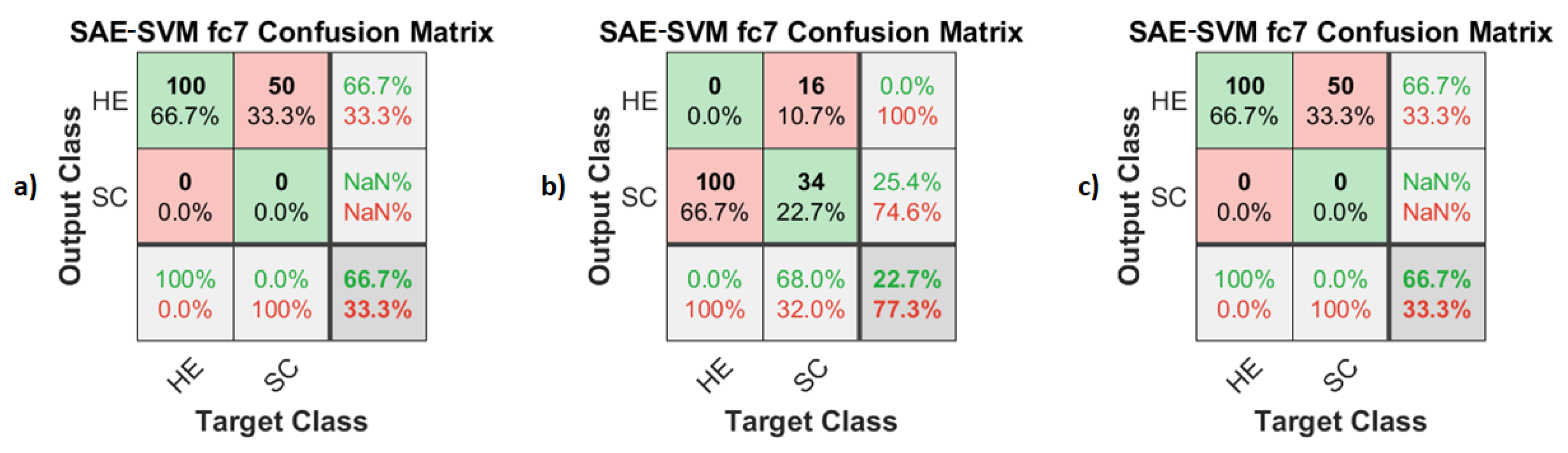
5.3. SAE-SVM Classifier

The sparse autoencoder added to the SVM classifier became an SEA-SVM classifier. While unsupervised extraction of important parameters seems favorable, the methods showed no consistent advantage over the SVM classifier in terms of classification performance. As illustrated by the results in Dataset 2, the autoencoder might even fail to extract useful features for discriminating between classes where the SVM classifier succeeds. Extracting features at fc7 ranked 5 / 5 in accuracy, PFA, and POD, mainly due to performance on the axial roller bearing dataset. In contrast, the SAE-SVM using fc6 was ranked 1 / 5 in PFA in fault classification for the axial roller bearing, but this result was accompanied by a 4 / 5 rank in POD. Introducing the autoencoder in addition to the SVM adds complexity in terms of tuning parameters and requires time and computational power to train. Combined with the results, this method is not recommended for classifying faults in roller bearings if using simple transfer learning.
Table 12 gives a comparative evaluation of the proposed fault classifiers for roller bearings, where + and + + indicate good and very good relative performance, while − and are the negative equivalents.

5.4. Comparison with Envelope Analysis

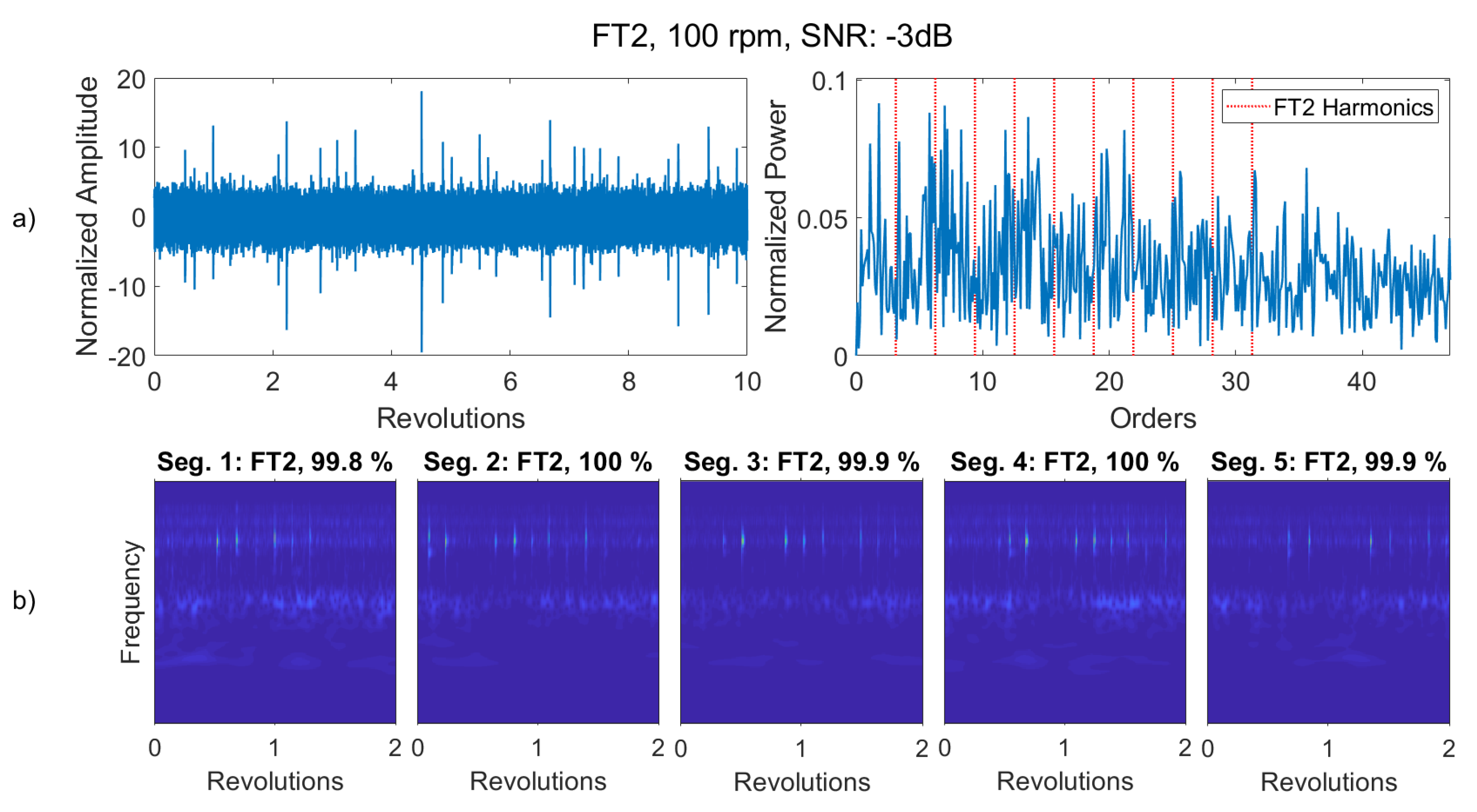
Envelope analysis has been commonly used in detecting bearing faults in industry. The performance of the proposed algorithms using machine learning was compared to those of using envelope analysis. In Dataset 1, the roller element fault (FT2) was more difficult to detect than the outer race fault; thus, we provide an example where FT2 at the lowest speed (100 rpm) was analyzed using envelope analysis. In the proposed classifiers, segments of two revolutions were used. To improve resolution in the envelope spectrum, five segments were combined so that total segment length was extended to 10 revolutions. As shown in Figure 13, even though transients were visible in the time domain waveform, no clear peak was visible in the envelope spectrum without further processing. However, the proposed method, here illustrated by the CNN classifier, can predict the correct class with above 99% probability. Envelope analysis would in this case require a certain expertise to perform further analysis.

6. Conclusions

A transfer learning approach to bearing fault classification using a pretrained convolution neural network (CNN) was proposed in this work. It was shown that the pretrained network can be fine tuned, or used to generate features for detecting bearing faults by other machine learning-based classifiers. Three classifiers based on CNN, support vector machine (SVM) and combined sparse autoencoder (SAE) and SVM algorithms were used to classify faults in axial and radial roller bearings using both vibration and acoustic emission signals.
The performance and robustness of the proposed method were investigated under different fault types, operating speed, and noise levels. The investigation shows that extracting features from the pretrained CNN directly, then using the SVM for classification, is the best option to detect faults in roller bearings in terms of robustness, easy implementation, and computational burden. Fine-tuning of the CNN scales well to multiclass classification problems, but yields lower accuracy than the SVM classifier. Combined with increased computational burden and more tunable hyperparameters, the CNN-based classifier is ranked as the second best option. Unsupervised dimensionality reduction using SEA to the extracted features from the pretrained CNN increases the computational burden and complexity of the SAE-SVM classifier for this application. It also has a negative effect on robustness and thus the accuracy of the classification.

Author Contributions

Conceptualization, M.H., H.V.K. and T.J.J.M.; formal analysis, M.H.; funding acquisition, K.G.R. and T.J.J.M.; investigation, M.H.; methodology, M.H.; software, M.H.; supervision, H.V.K., K.G.R., T.I.W. and T.J.J.M.; writing, original draft, M.H. and H.V.K.; writing, review and editing, H.V.K., K.G.R. and T.I.W. The first author produced the results and mainly wrote the paper. The other authors contributed with comments and suggestions.

Funding

The research presented in this paper has received funding from the Norwegian Research Council, SFI Offshore Mechatronics, Project Number 237896.

Conflicts of Interest

The authors declare no conflict of interest. The founding sponsors had no role in the design of the study; in the collection, analyses, or interpretation of data; in the writing of the manuscript; nor in the decision to publish the results.

References

  1. Albrecht, P.; Appiarius, J.; McCoy, R.E.; Owen, D.S. Assessment of the Reliability of Motors in Utility Applications - Updated. IEEE Trans. Energy Convers. 1986, 1, 39–46. [Google Scholar] [CrossRef]
  2. ISO 18436-2:2014 International Organization for Standardization. 2014. Available online: https://www.iso.org/standard/50447.html (accessed on 16 December 2018).
  3. Jacop, A.; Khang, H.V.; Robbersmyr, K.G.; Cardoso, A.J.M. Bearing fault detection for drivetrains using adaptive filters based wavelet transform. In Proceedings of the IEEE International Conference on Electrical Machines and Systems (ICEMS), Sydney, NSW, Australia, 11–14 August 2017; pp. 1–6. [Google Scholar] [CrossRef]
  4. Qiu, H.; Lee, J.; Lin, J.; Yu, G. Wavelet filter-based weak signature detection method and its application on rolling element bearing prognostics. J. Sound Vib. 2006, 289, 1066–1090. [Google Scholar] [CrossRef]
  5. Hemmer, M.; Waag, T.I. A Comparison of Acoustic Emission and Vibration Measurements for Condition Monitoring of an Offshore Drilling Machine. In Proceedings of the Annual Conference of the Prognostics and Health Management Society, St. Petersburg, FL, USA, 2–5 October 2017; pp. 278–285. [Google Scholar]
  6. Du, Z.; Chen, X.; Zhang, H.; Yan, R. parse feature identification based on union of redundant dictionary for wind turbine gearbox fault diagnosis. IEEE Trans. Ind. Electron. 2015, 10, 6594–6605. [Google Scholar] [CrossRef]
  7. Jung, D.; Sundström, C. A Combined Data-Driven and Model-Based Residual Selection Algorithm for Fault Detection and Isolation. IEEE Trans. Control Syst. Technol. 2017, 1–15. [Google Scholar] [CrossRef]
  8. Dai, X.; Gao, Z. From model, signal to knowledge: A data-driven perspective of fault detection and diagnosis. IEEE Trans. Ind. Inf. 2013, 4, 2226–2238. [Google Scholar] [CrossRef]
  9. Gao, Z.; Cecati, C.; Ding, S.X. A Survey of Fault Diagnosis and Fault-Tolerant Techniques—Part I: Fault Diagnosis With Model-Based and Signal-Based Approaches. IEEE Trans. Ind. Inf. 2015, 62, 3757–3767. [Google Scholar] [CrossRef] [Green Version]
  10. Gao, Z.; Cecati, C.; Ding, S.X. A Survey of Fault Diagnosis and Fault-Tolerant Techniques-Part II: Fault Diagnosis with Knowledge-Based and Hybrid/Active Approaches. IEEE Trans. Ind. Inf. 2015, 62, 3768–3774. [Google Scholar] [CrossRef]
  11. Niu, G. Data-Driven Technology for Engineering Systems Health Management: Design Approach, Feature Construction, Fault Diagnosis, Prognosis, Fusion and Decision; Springer: Berlin, Germany, 2016. [Google Scholar]
  12. Baydar, N.; Chen, Q.; Ball, A.; Kruger, U. Detection of incipient tooth defect in helical gears using multivariate statistics. Mech. Syst. Signal Process. 2001, 15, 303–321. [Google Scholar] [CrossRef]
  13. Konar, P.; Chattopadhyay, P. Bearing fault detection of induction motor using wavelet and support vector machines (SVMs). Appl. Soft Comput. 2011, 11, 4203–4211. [Google Scholar] [CrossRef]
  14. Senanayaka, J.S.L.; Kandukuri, S.T.; Khang, H.V.; Robbersmyr, K.G. Early detection and classification of bearing faults using support vector machine algorithm. In Proceedings of the 2017 IEEE Workshop on Electrical Machines Design, Control and Diagnosis (WEMDCD), Nottingham, UK, 20–21 April 2017; pp. 250–255. [Google Scholar] [CrossRef]
  15. Senanayaka, J.S.L.; Khang, H.V.; Robbersmyr, K.G. Towards online bearing fault detection using envelope analysis of vibration signal and decision tree classification algorithm. In Proceedings of the IEEE International Conference on Electrical Machines and Systems (ICEMS), Sydney, NSW, Australia, 11–14 August 2017; pp. 1–6. [Google Scholar]
  16. Zhang, R.; Tao, H.; Wu, L.; Guan, Y. Transfer Learning with Neural Networks for Bearing Fault Diagnosis in Changing Working Conditions. IEEE Access 2017, 5, 14347–14357. [Google Scholar] [CrossRef]
  17. Wu, L.; Yao, B.; Peng, Z.; Guan, Y. Fault Diagnosis of roller bearings based on a wavelet neural network and manifold learning. Appl. Sci. 2017, 7, 158. [Google Scholar] [CrossRef]
  18. Susto, G.A.; Schirru, S.P.; McLoone, S.; Beghi, A. Machine learning for predictive maintenance: A multiple classifier approach. IEEE Trans. Ind. Inf. 2015, 11, 14347–14357. [Google Scholar] [CrossRef]
  19. Krizhevsky, A.; Sutskever, I.; Hinton, G.E. ImageNet Classification with Deep Convolutional Neural Networks. In Advances in Neural Information Processing Systems; MIT Press: Cambridge, MA, USA, 2012; pp. 1097–1105. [Google Scholar]
  20. Shelhamer, E. AlexNet Model. Available online: https://github.com/BVLC/caffe/tree/master/models/bvlc_alexnet (accessed on 28 September 2018).
  21. Senanayaka, J.S.L.; Khang, H.V.; Robbersmyr, K.G. Multiple Fault Diagnosis of Electric Powertrains under Variable Speeds using Convolutional Neural Networks. In Proceedings of the IEEE ICEM, Alexandroupoli, Greece, 3–6 September 2018; pp. 1932–1938. [Google Scholar] [CrossRef]
  22. Suykens, J.; Vandewalle, J. Least Squares Support Vector Machine Classifiers. Neural Process. Lett. 1999, 9, 293–300. [Google Scholar] [CrossRef]
  23. Hosseini-Asl, E.; Zurada, J.M.; Nasraoui, O. Deep Learning of Part-Based Representation of Data Using Sparse Autoencoders With Nonnegativity Constraints. IEEE Trans. Neural Netw. Learn. Syst. 2016, 27, 2486–2498. [Google Scholar] [CrossRef] [PubMed]
  24. Jia, F.; Lei, Y.; Lu, N.; Xing, S. Deep normalized convolutional neural network for imbalanced fault classification of machinery and its understanding via visualization. Mech. Syst. Signal Process. 2018, 110, 14347–14357. [Google Scholar] [CrossRef]
Figure 1. Methodology visualization. SAE, sparse autoencoder.
Designs 02 00056 g001
Figure 2. Simplified illustration of the AlexNet architecture.
Designs 02 00056 g002
Figure 3. Radial bearing test rig.
Designs 02 00056 g003
Figure 4. Faults in the test bearing: (a) outer race (OR) fault and (b) rolling element (RE) fault.
Designs 02 00056 g004
Figure 5. (a) Schematic drawing of the in-house axial bearing test rig. (b) Acoustic emission sensor placement.
Designs 02 00056 g005
Figure 6. (a) Schematic drawing of the damage mechanism. (b) Scratches on the axial bearing roller end.
Designs 02 00056 g006
Figure 7. Comparison of the time-waveform and CWT at (a) 100 rpm and (b) 1000 rpm.
Designs 02 00056 g007
Figure 8. Fault Type 1 vibration signal with an outer race fault at 4 increasing SNR levels.
Designs 02 00056 g008
Figure 9. Dataset 1 preprocessing.
Designs 02 00056 g009
Figure 10. Acoustic emission signal during damage and CWT spectrograms of Segments 3 and 9.
Designs 02 00056 g010
Figure 11. Confusion matrices for Dataset 1, 75% training data, Fault Type 2 at SNR3 and SNR4. (a) CNN classifier, (b) SVM classifier at fc6, and (c) SAE-SVM classifier at fc6.
Designs 02 00056 g011
Figure 12. Confusion matrices for Dataset 2 with (a) 75%, (b) 50%, and (c) 25% training data.
Designs 02 00056 g012
Figure 13. (a) Time domain signal and the envelope spectrum for the faulty roller element at 100 rpm. (b) Classification of the corresponding spectrograms using the CNN classifier.
Designs 02 00056 g013
Table 1. CNN settings.
SolverStochastic Gradient Descent with Momentum (SGDM)
Training epochs50
Initial learning Rate, overall 10 3
Initial learning Rate, fc8 0.02
Learning Rate Drop Factor0.2
Learning Rate Drop Period10
Table 2. SVM settings.
Feature Layersfc6 and fc7
KernelLinear
StandardizationUnit mean and variance
SolverIterative Single Data Algorithm (ISDA)
Outlier fraction0.0
Table 3. SAE settings.
Hidden layer size100
Training algorithmScaled conjugate gradient descent
Training epochs2500
Encoder transfer functionLogistic sigmoid function
Decoder transfer functionLogistic sigmoid function
L 2 Weight Regularization0.001
Loss functionMean squared error with L 2 and sparsity regularization
Sparsity proportion0.05
Table 4. Radial test data. HE, healthy.
rpm1002003004005007501000Total
Load (kN)5555555
No. of HE60606060606060420
No. of RE1010101010101070
No. of OR1010101010101070
Total80808080808080560
Table 5. Radial training/validation data distribution.
TrainingValidation
LabelNumber of Images75%50%25%25%
Healthy420315210105105
Damage140105703535
Total560420280140140
Table 6. Axial training data.
TrainingValidation
LabelNumber of Images75%50%25%25%
Healthy400300200100100
Damage2001501005050
Total600450300150150
Table 7. SNR levels.
SNR1Reference (no added noise)
SNR20 dB
SRN3−3 dB
SNR4−10 dB
Table 8. Validation accuracy: Dataset 1. FT, fault type.
FT1-ORFT2-RE
Training Data SNR1SNR2SNR3SNR4SNR1SNR2SNR3SNR4
75%CNN99.3%100.0%100.0%97.9%100.0%98.6%92.9%89.3%
SVM fc6100.0%100.0%100.0%96.4%100.0%97.9%94.3%87.1%
SVM fc7100.0%100.0%100.0%95.7%99.3%97.1%95.0%82.1%
SAE-SVM fc6100.0%98.6%100.0%93.6%100.0%85.7%95.0%82.1%
SAE-SVM fc7100.0%100.0%100.0%90.0%99.3%95.7%93.6%85.0%
50%CNN100.0%100.0%100.0%95.7%99.3%97.1%97.1%85.0%
SVM fc6100.0%100.0%100.0%97.1%98.6%97.1%95.0%86.4%
SVM fc7100.0%100.0%100.0%95.7%98.6%95.0%92.1%80.0%
SAE-SVM fc6100.0%100.0%100.0%95.0%99.3%95.0%94.3%78.6%
SAE-SVM fc7100.0%100.0%100.0%95.0%99.3%92.9%90.0%79.3%
25%CNN98.7%100.0%98.6%86.4%100.0%91.4%92.1%86.4%
SVM fc6100.0%100.0%100.0%95.7%99.3%96.4%95.0%85.0%
SVM fc7100.0%100.0%100.0%95.0%98.6%96.4%94.3%85.7%
SAE-SVM fc6100.0%100.0%99.9%82.1%98.6%97.1%92.1%69.3%
SAE-SVM fc7100.0%100.0%99.3%87.1%97.9%93.6%90.7%78.6%
Table 9. Validation accuracy: Dataset 2.
Training DataCNNSVM fc6SVM fc7SAE-SVM fc6SAE-SVM fc7
7597.3%98.7%98.7%97.3%66.7%
5098.7%100.0%99.3%94.7%22.7%
2597.3%98.0%96.7%95.3%66.7%
Table 10. Mean accuracy for each classifier.
Accuracy
CNN96.93%
SVM fc697.81%
SVM fc797.04%
SAE-SVM fc694.89%
SAE-SVM fc773.23%
Table 11. Mean probability of false alarm (PFA) and probability of detection (POD) across SNR and training data size.
PFAPOD
RADIAL FT1RADIAL FT2AXIALMEANRADIAL FT1RADIAL FT2AXIALMEAN
CNN1.19%1.98%2.00%1.72%95.71%82.38%96.00%91.36%
SVM fc60.79%2.54%1.00%1.44%98.81%85.00%98.67%94.16%
SVM fc70.87%3.81%2.33%2.34%98.10%82.86%99.33%93.43%
SAE-SVM fc62.22%4.92%0.67%2.60%96.19%77.14%88.67%87.33%
SAE-SVM fc72.22%4.52%33.33%13.36%97.14%78.81%22.67%66.21%
Table 12. Classifier evaluation.
AccuracyRobustnessImplementationComputational Burden
CNN+++
SVM+++++
SAE-SVM

