PV Microgrid Design for Rural Electrification


Abstract
:
1. Introduction
- Being located in areas with difficult terrain such as hills, forests, deserts and islands. Being part of a protected forest area could isolate the village and prevent live conductors from being drawn through it.
- Being located far from the nearest existing grid.
- Very low population (below 500) and low number of households (ranging between 2 and 200).
- Low power demand, probably even in the near future, as the loads are mostly lighting.
- Minimal transport and communication facilities.
- Low income level and low affordability.
- Poor literacy levels and technical skills.
2. The Design Problem
- Voltage drop limits the design: The loads are distributed over large distances, which increase the voltage drop at the extreme consumer point in a radial system.
- Losses costs are high: Moving relatively small amounts of power over long distances results in losses which are high in proportion to the amount of power delivered.
- Layout and customers are restricted to the road network.
- Loads vary from very small single-phase to medium sized three-phase. Water pumps for irrigation purpose may require three-phase supply.
- Reliability requirements are below average.
- What should be the network (microgrid) structure?
- What should be the size of the central PV system?
- Where the PV system should be located?
- What should be the specifications of cables, protective equipment?
- Spatially distributed ‘point’ loads and estimate of its magnitudes
- Location details and/or local resource availability
- Roads and other obstacles
- Expected load growth
- Cost of PV system and power network feeders
- ∙
- Installation cost
- ∙
- Operating cost
- The minimum PV system and battery bank size determined is adequate to ensure continuity of supply to the load
- Voltage at each bus/node should be within limits
- Feeder capacity should not be exceeded
- The energy losses are minimized
- The PV system design is based on parameters of practical components.
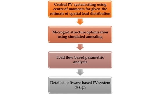
3. Methodology
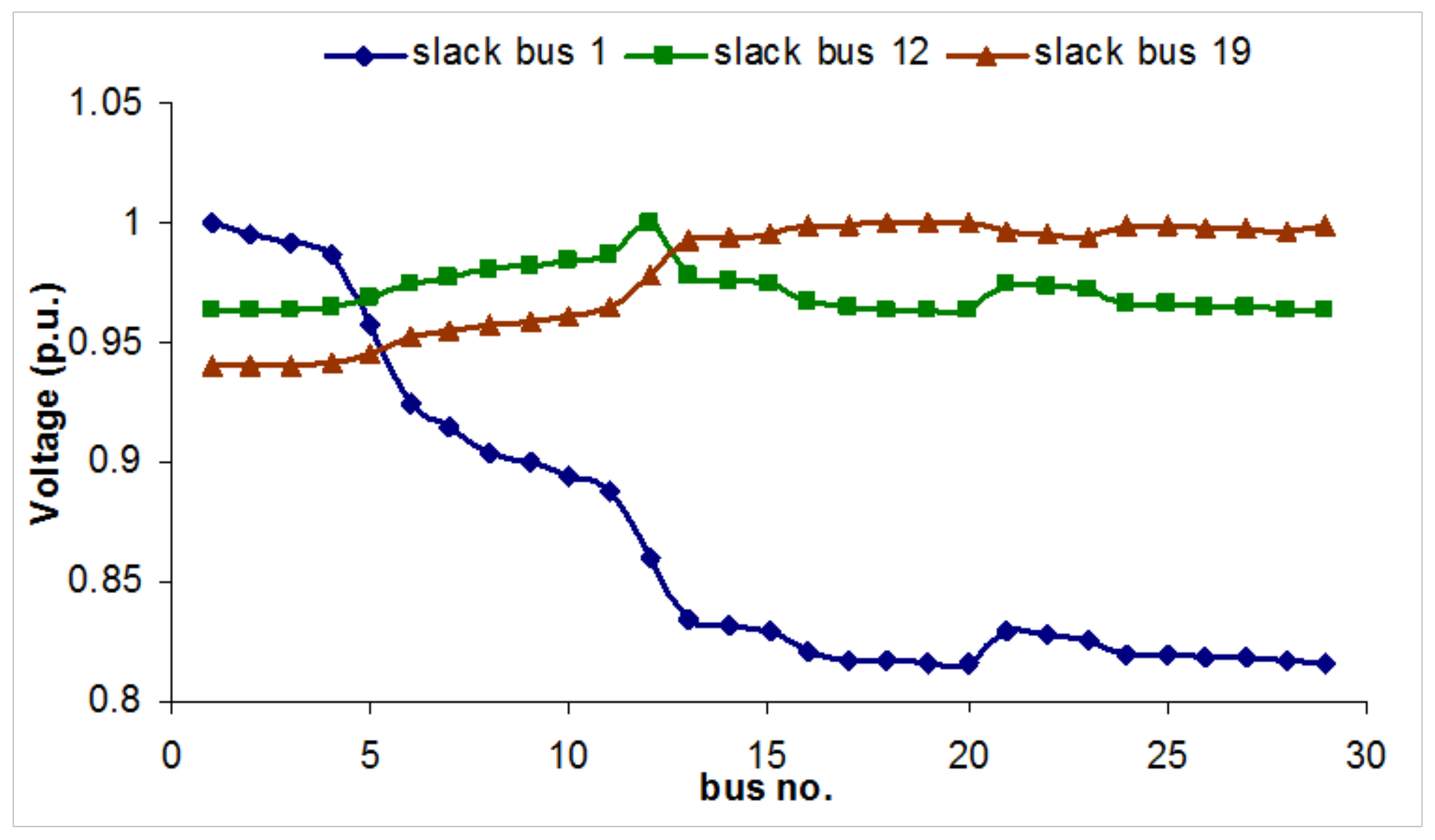
- Siting of source PV system
- Size of PV system
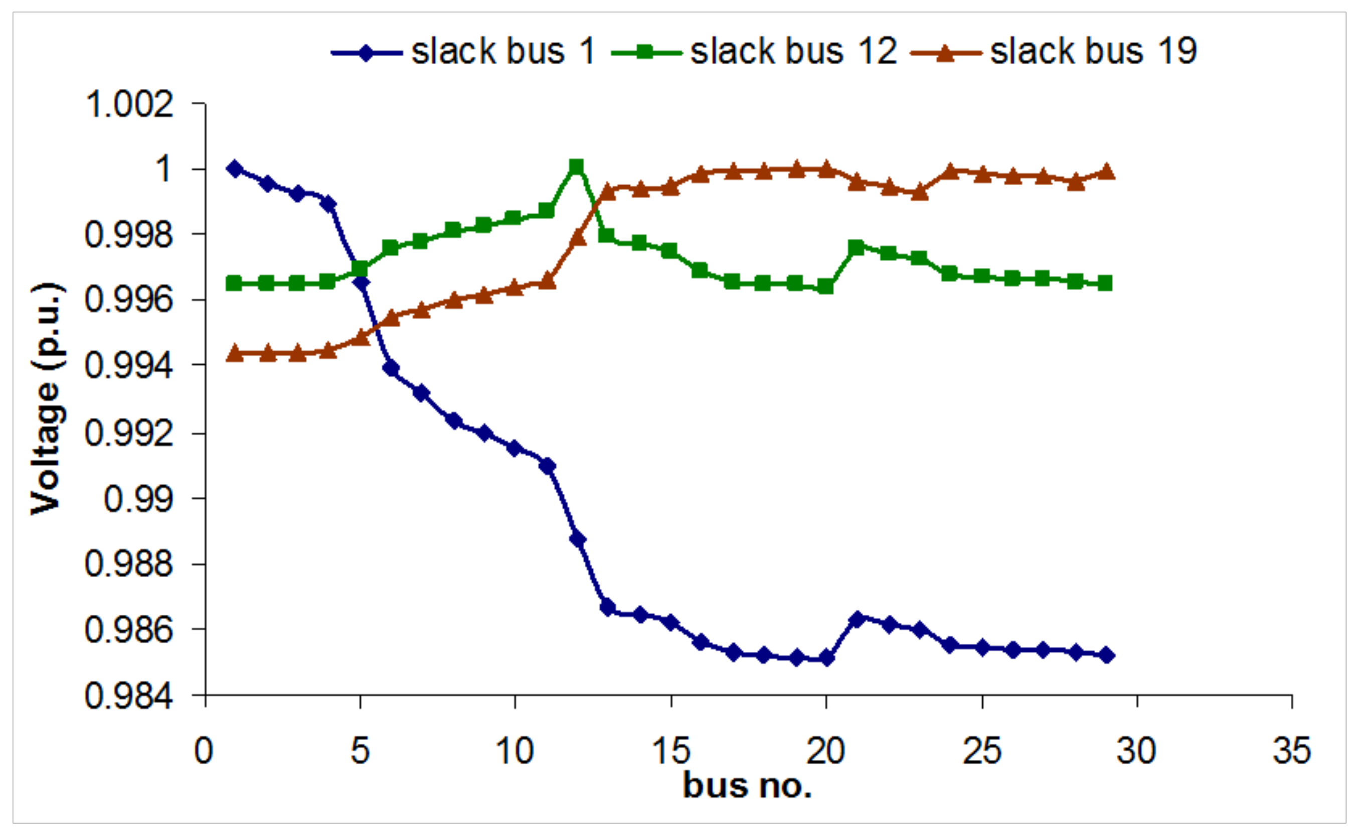
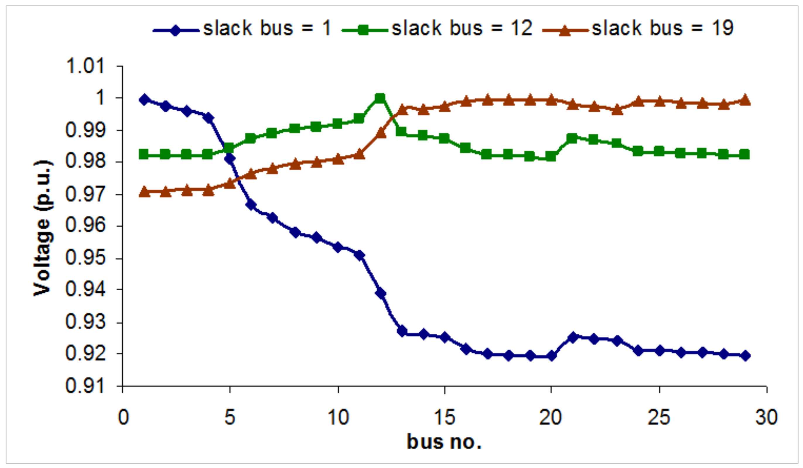
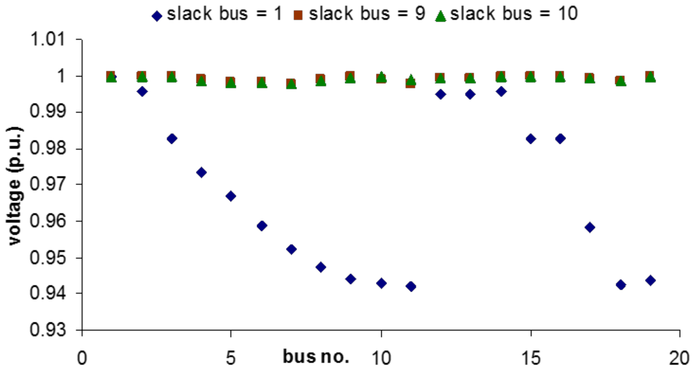
- Slack bus voltage (p.u.)
3.1. Case Study Systems
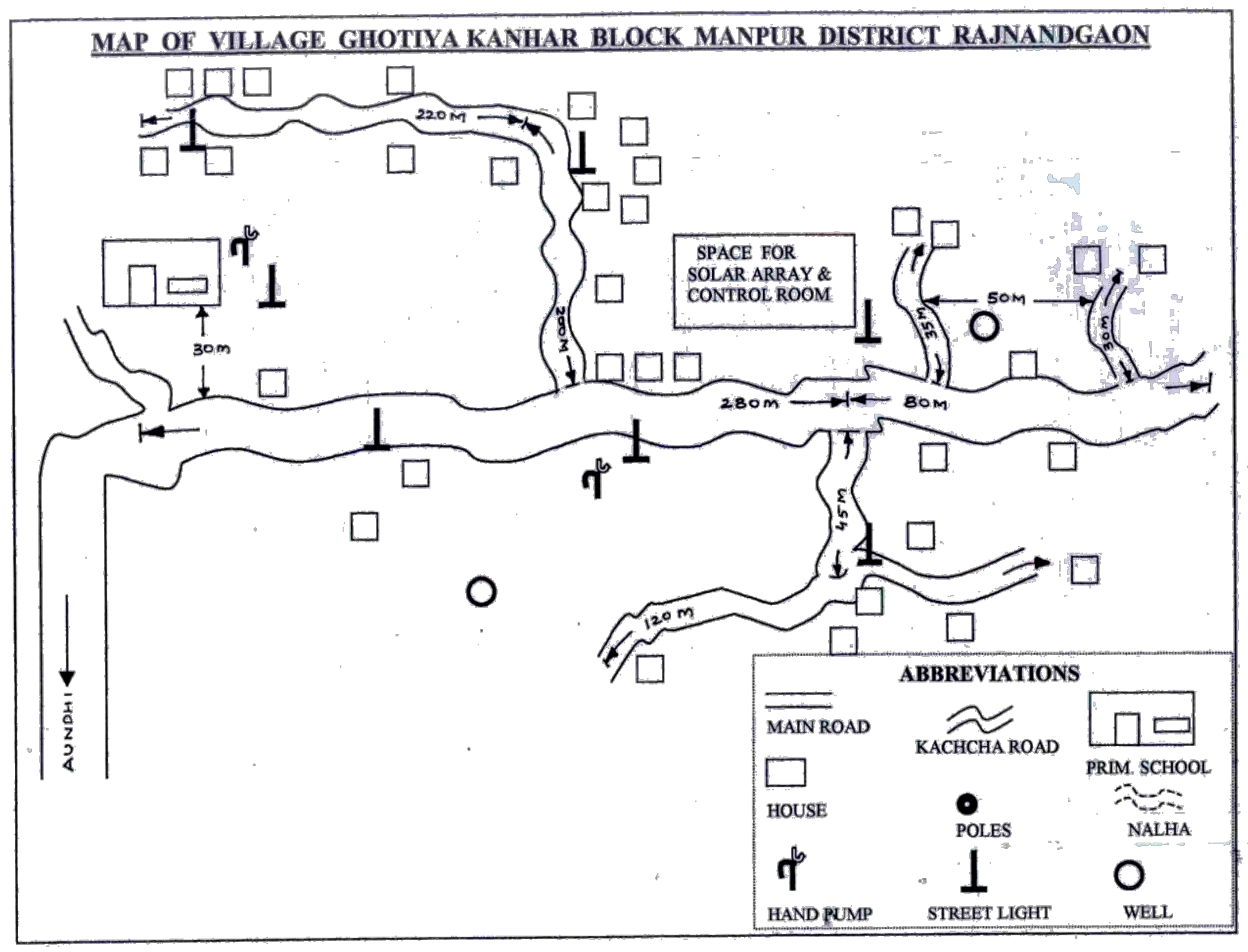
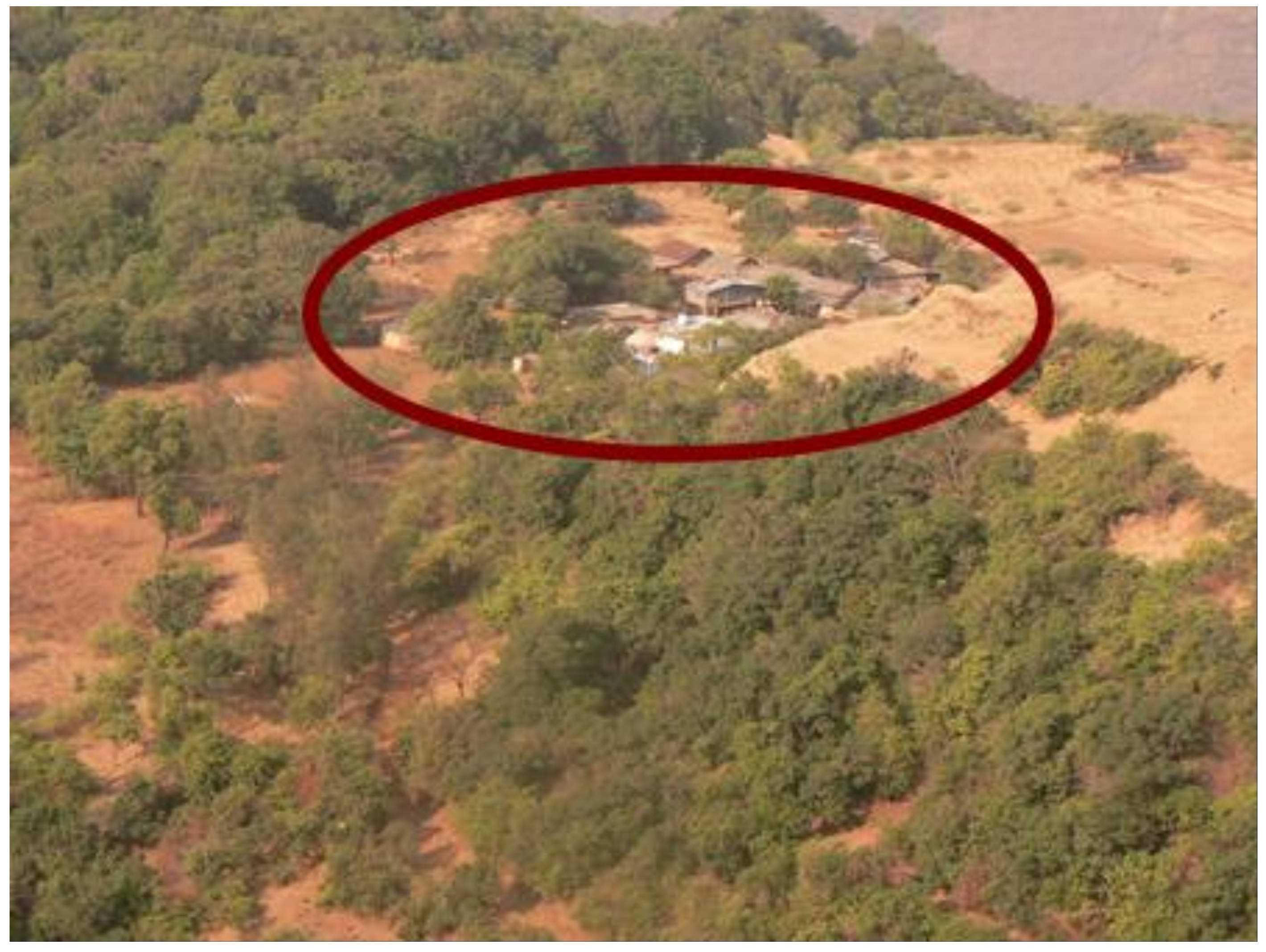
3.1.1. Ghotiya Village in Raipur, Chattisgarh
3.1.2. Rajmachi Village near Lonawala, Maharashtra
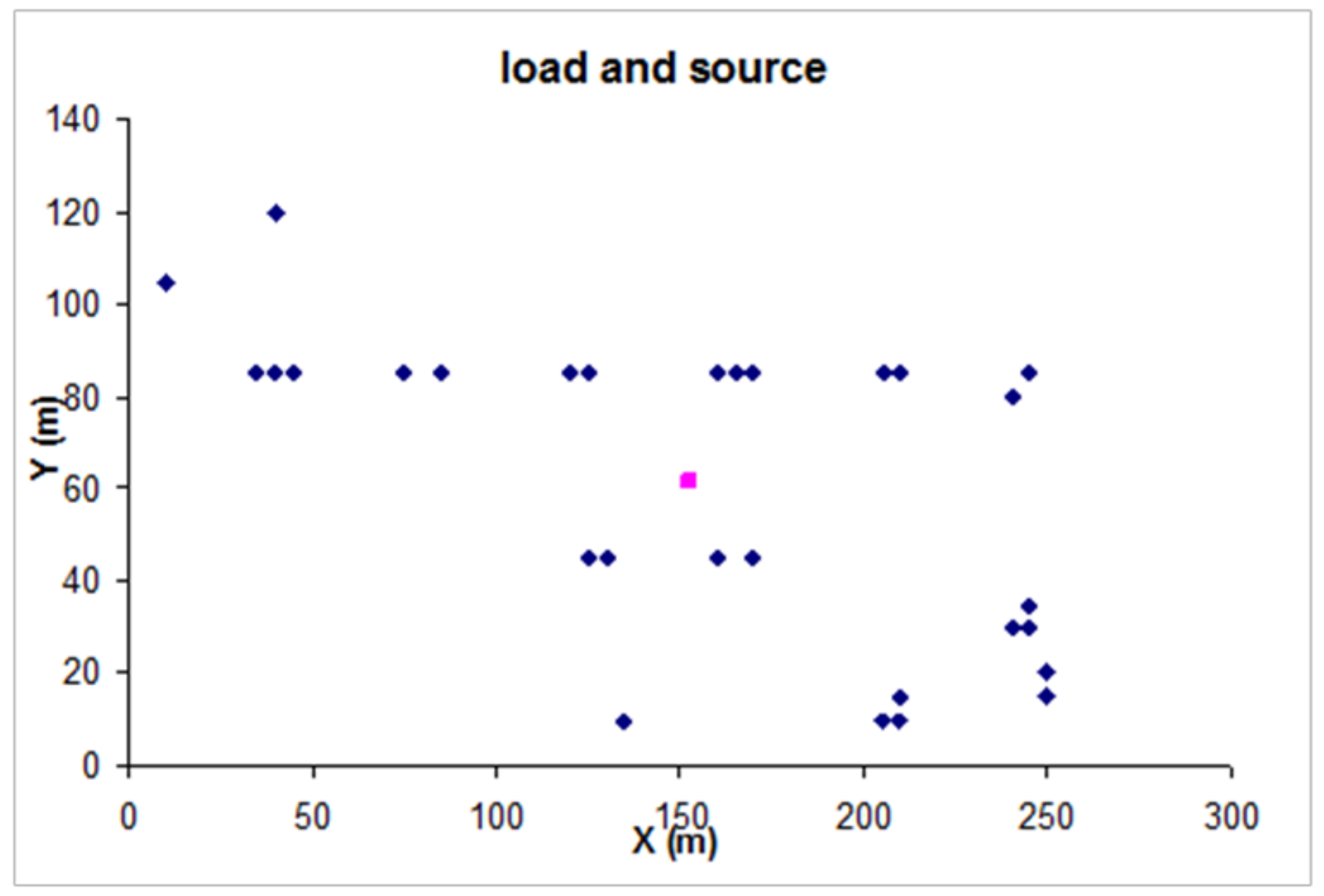
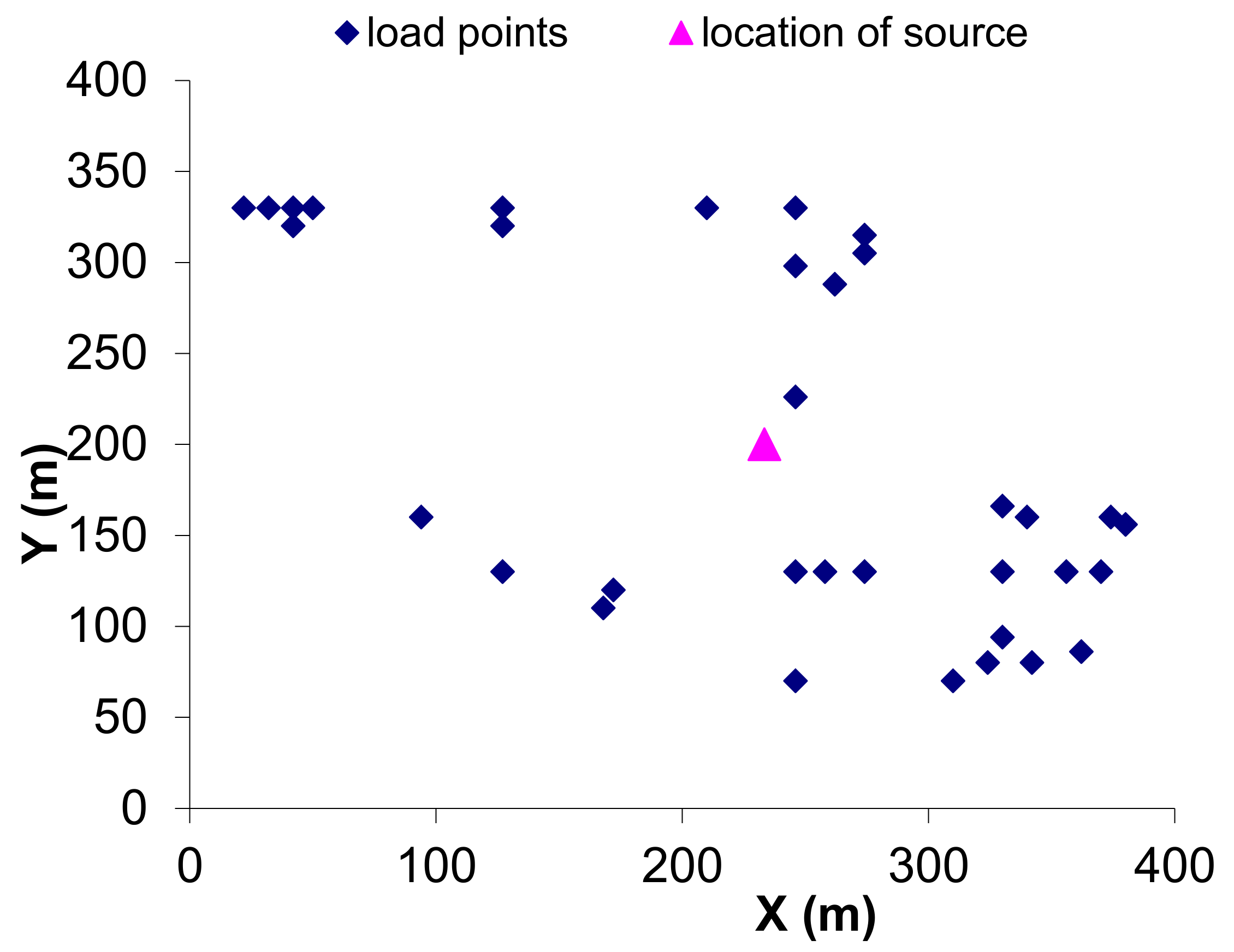
3.2. PV System Location Siting Using Centre of Moments
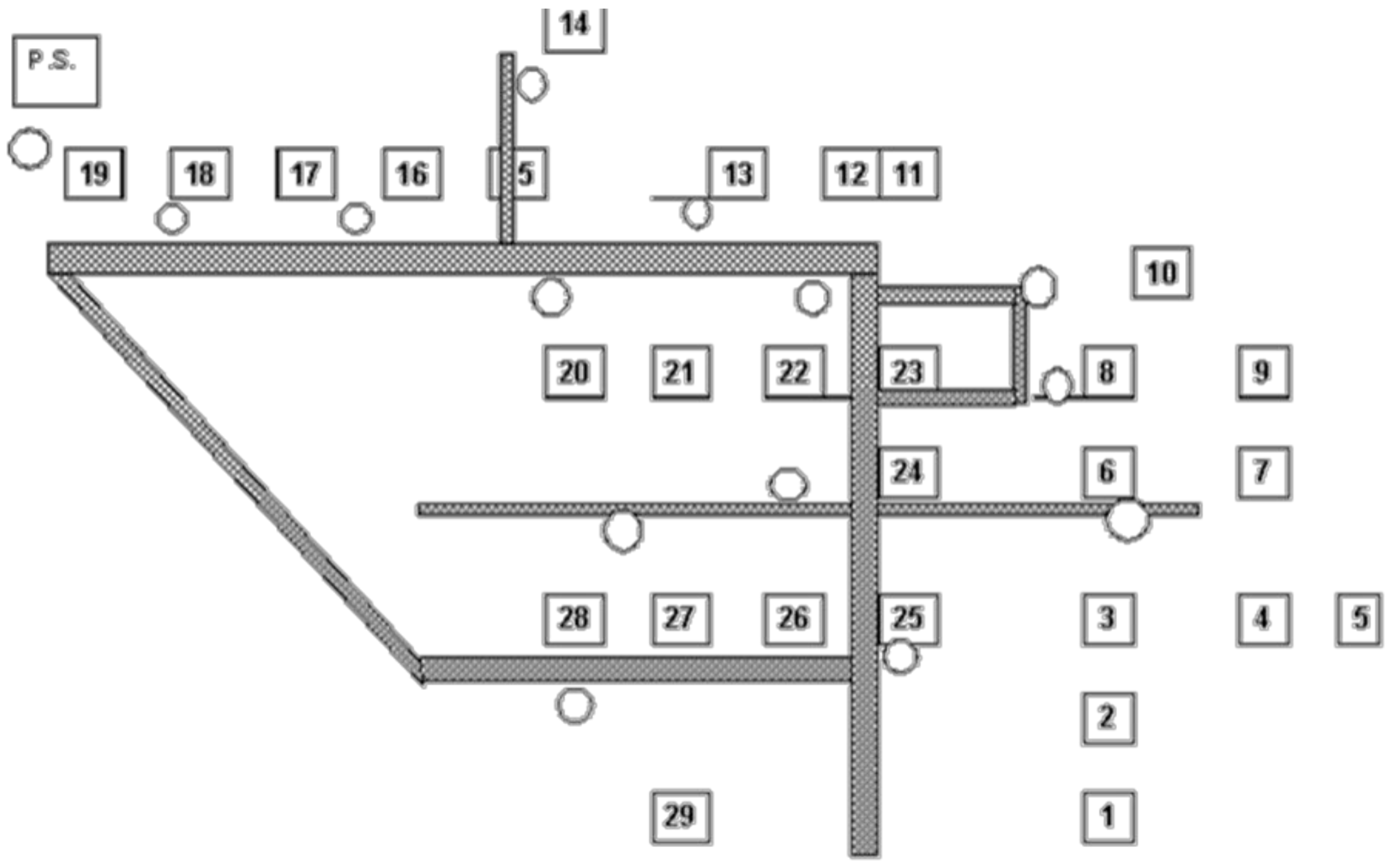
3.3. Network Topology Design
- Identify all the geographic constraints; areas that cannot be crossed, areas where construction is difficult etc.
- Identify all special opportunities; diagonal routes which contribute to lower cost.
- Identify a set of load points on the periphery of the area to be served by the feeder, as well as a load point that is the “worst case” in terms of each constraint
- One by one for each load points identified in step 3, work backward from it toward the substation (power source) trying to find out the shortest route(s). As feeders generally follow roads it is better to consider than (X and Y are the feeder lengths along the two coordinates of the site map).
- As a shortest path from each point is traced, commonalities among the paths can be used as major trunk or branch routes.
- the type of source and cost of generating electricity
- the costs of running wire across different types of terrain
- the maximum low voltage line length. This input restricts the length of low voltage wire runs. It refers to the length of wire between a load point and the transformer to which it is connected. This restriction is meant to limit voltage drops and line losses.
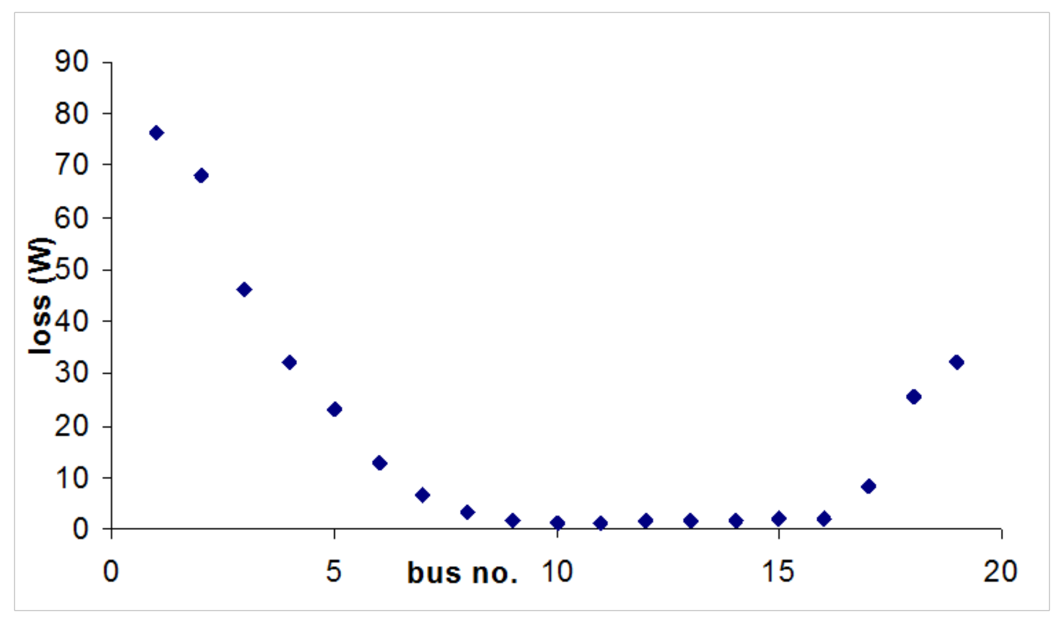
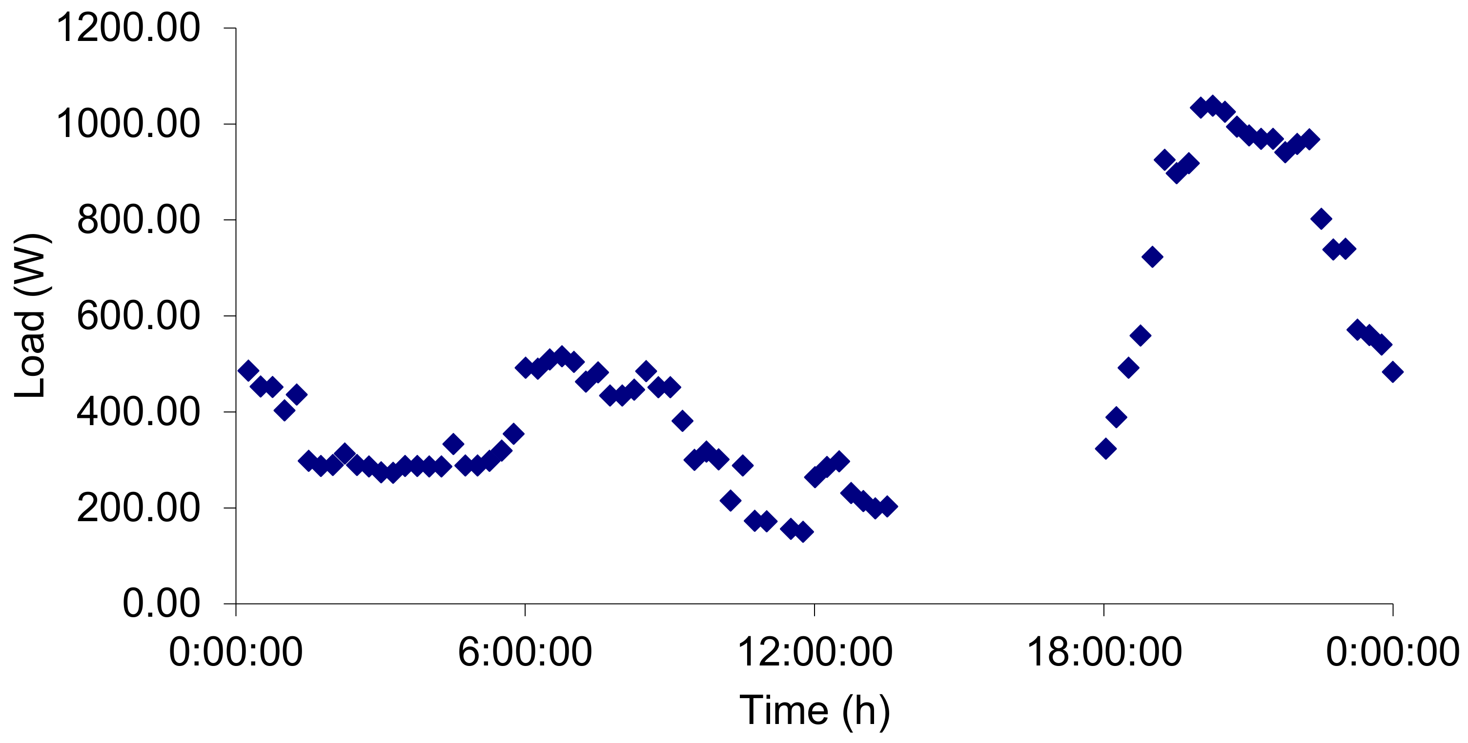
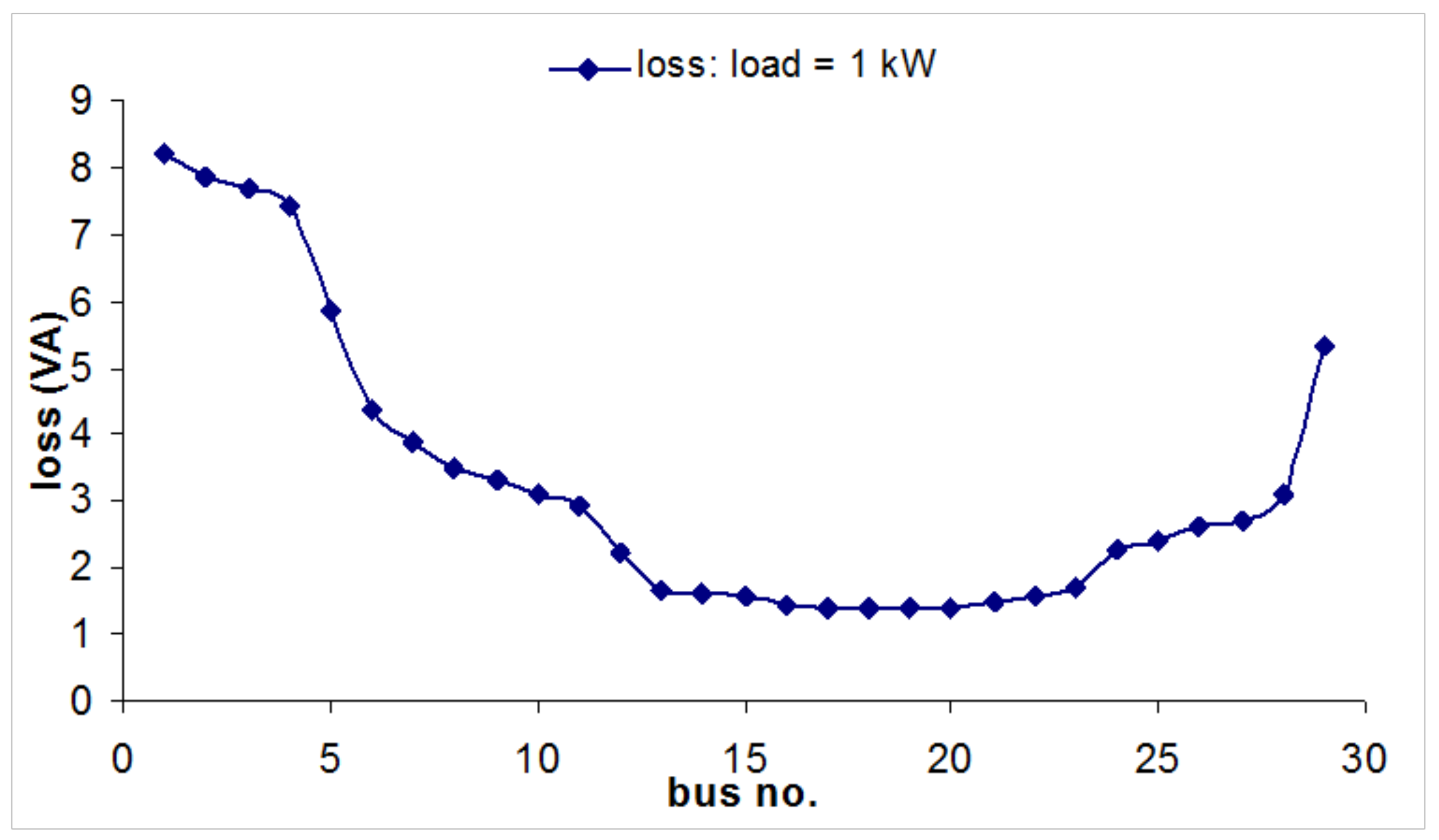
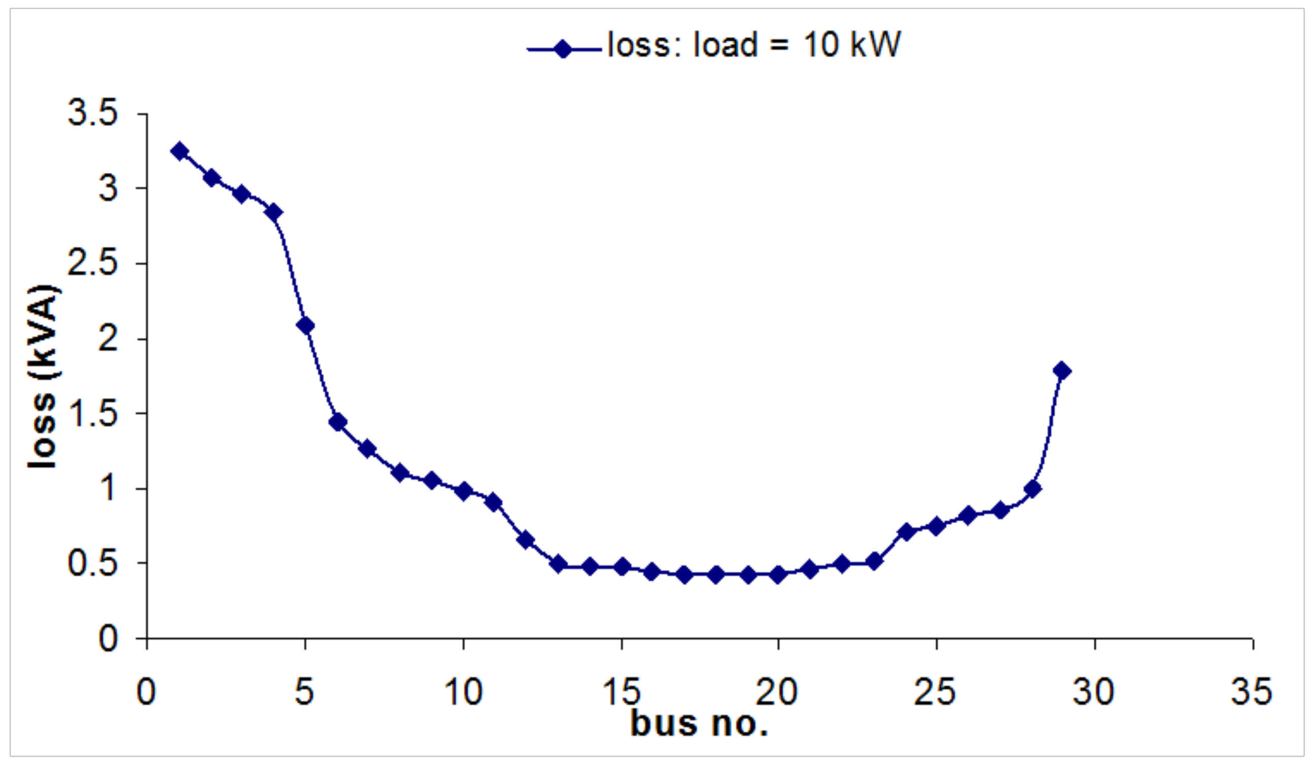
3.4. Parametric Analysis Based on Load Flow
- Voltage magnitudes and angles at all nodes of the feeder
- Line flow in each line section specified in kW and kVAr, amps and degree, or amps and power factor
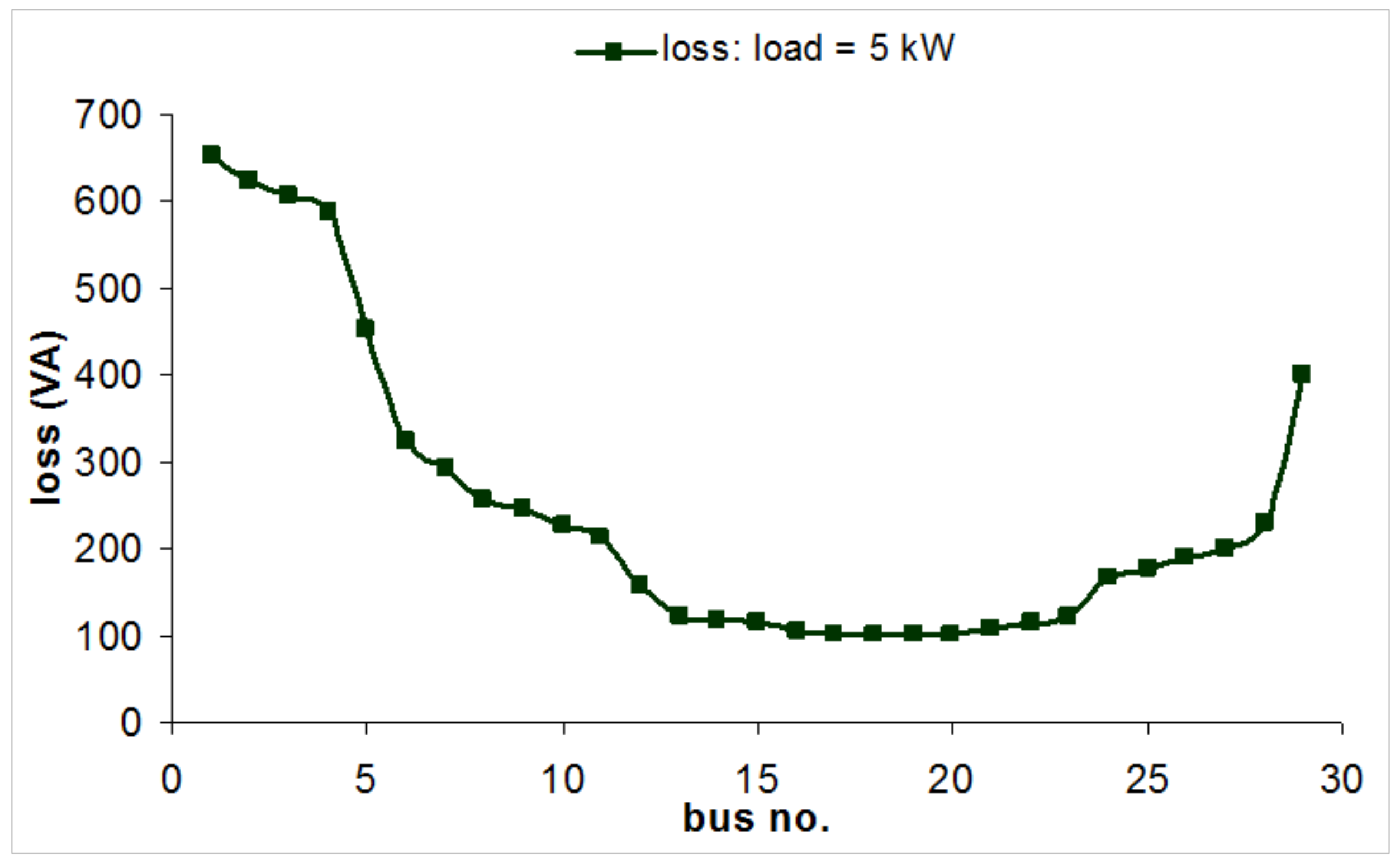
- Power loss in each line section
- Total feeder input kW and kVAr
- Total feeder power loss
- Load kW and kVAr based upon the specified model for the load.
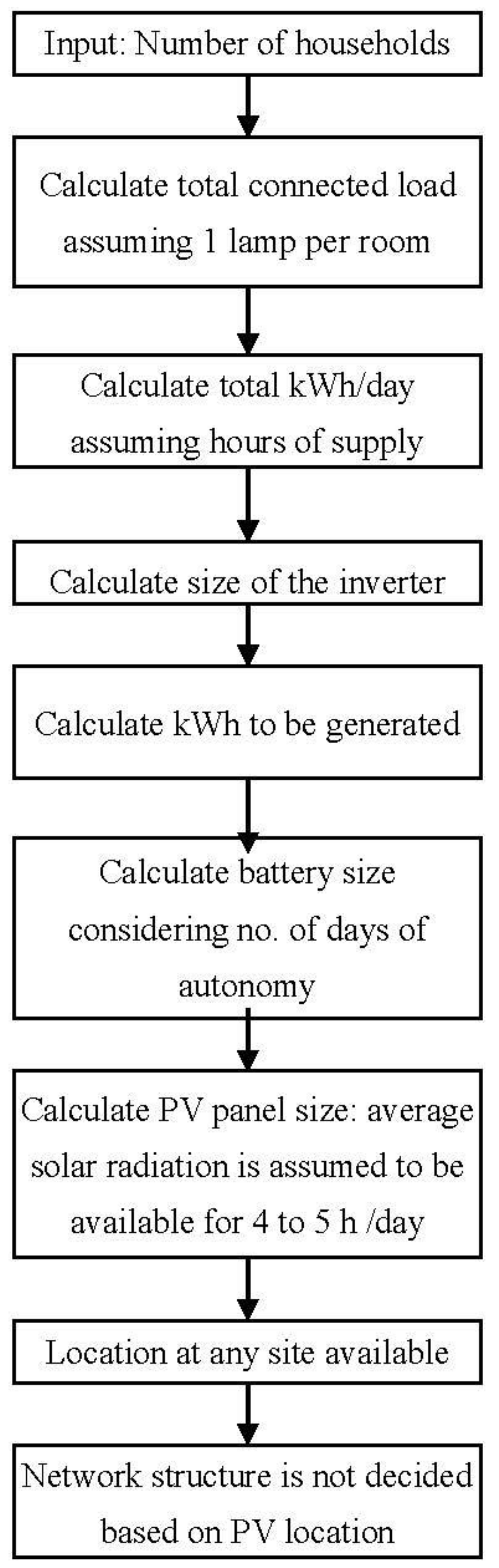
3.5. PV System Sizing
3.5.1. Pre-Sizing
3.5.2. Detailed Design
4. Results and Discussion
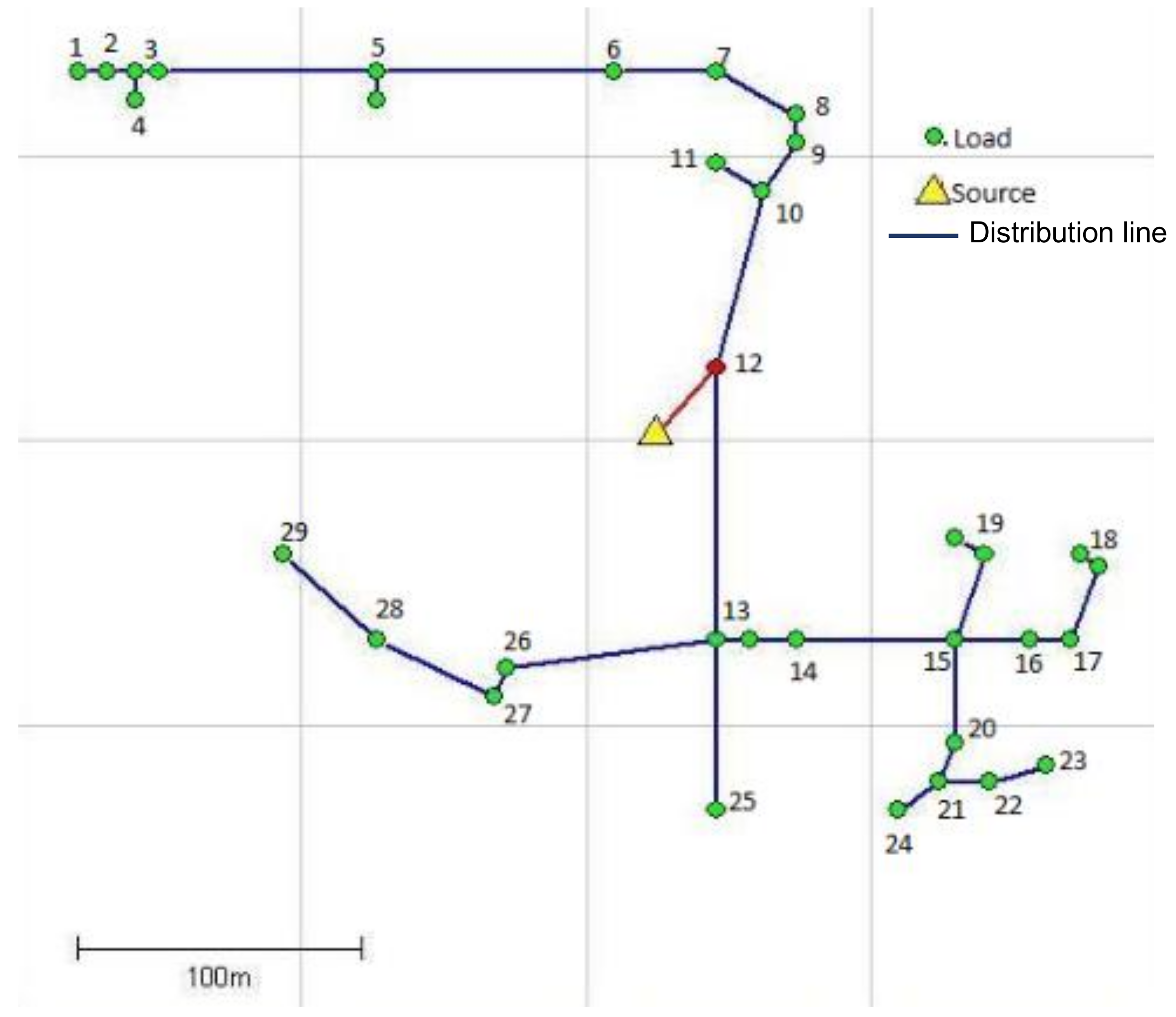
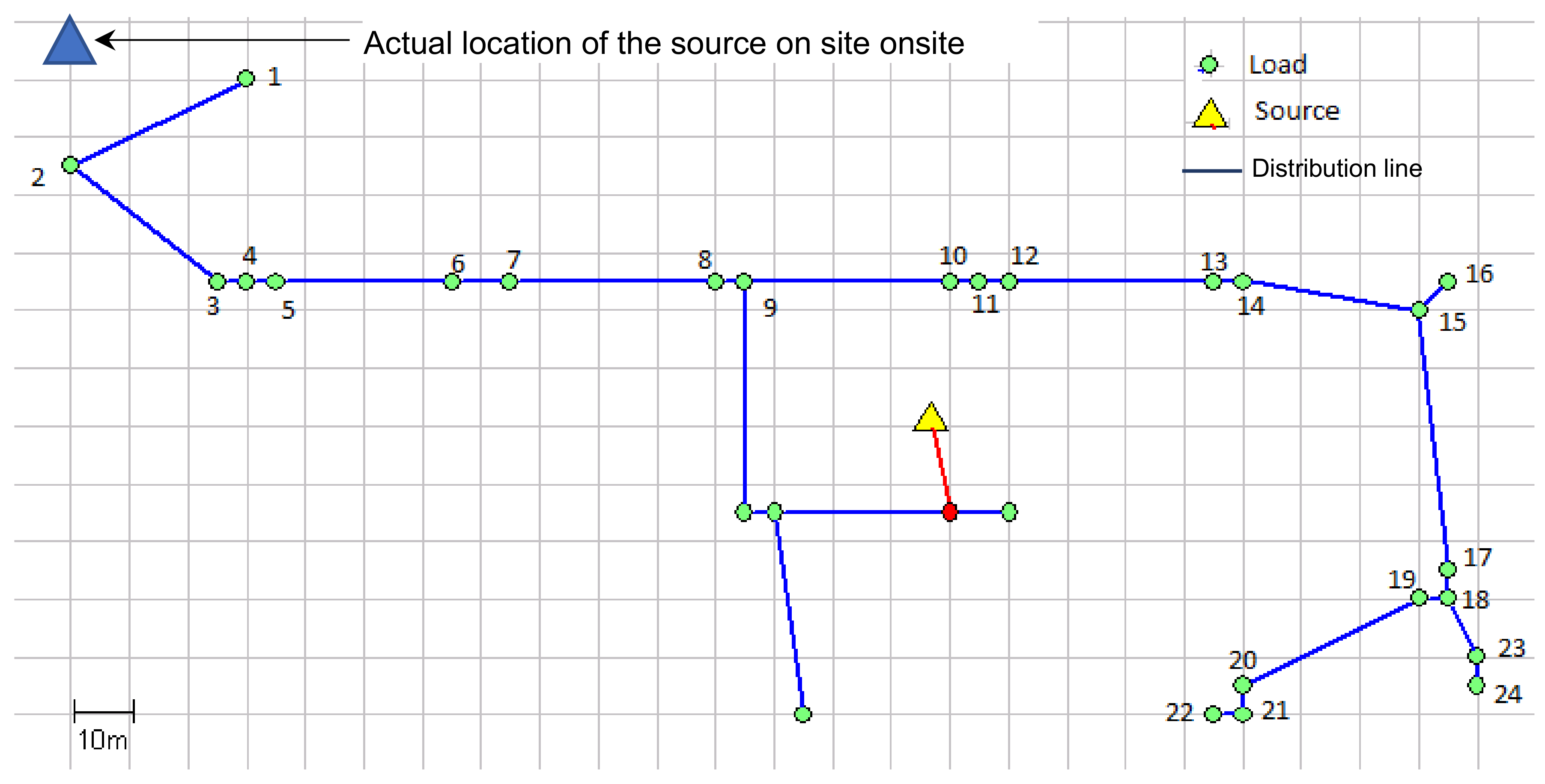
4.1. Location of PV System and Determination of Network Structure
4.1.1. Location of Central PV System in Terms of Spatial Distribution of Load
4.1.2. Determination of Network Topology Using Simulated Annealing
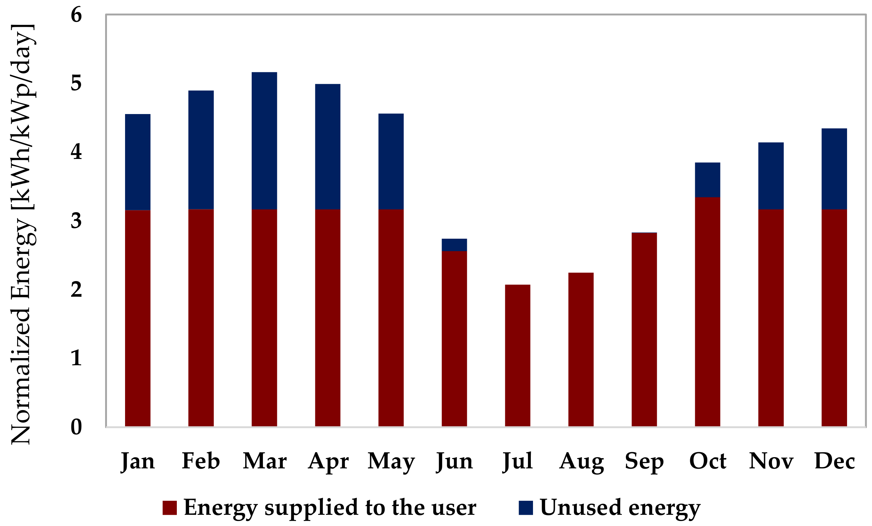
4.1.3. Parametric Analysis Using Load Flow
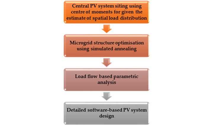
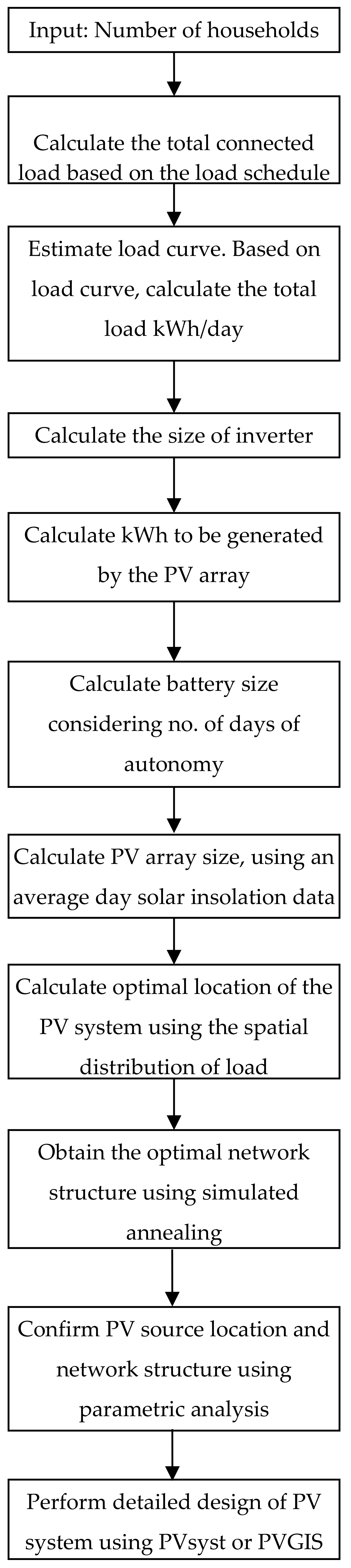
5. PV Microgrid Design Method for Rural Electrification
Illustration of Proposed Method
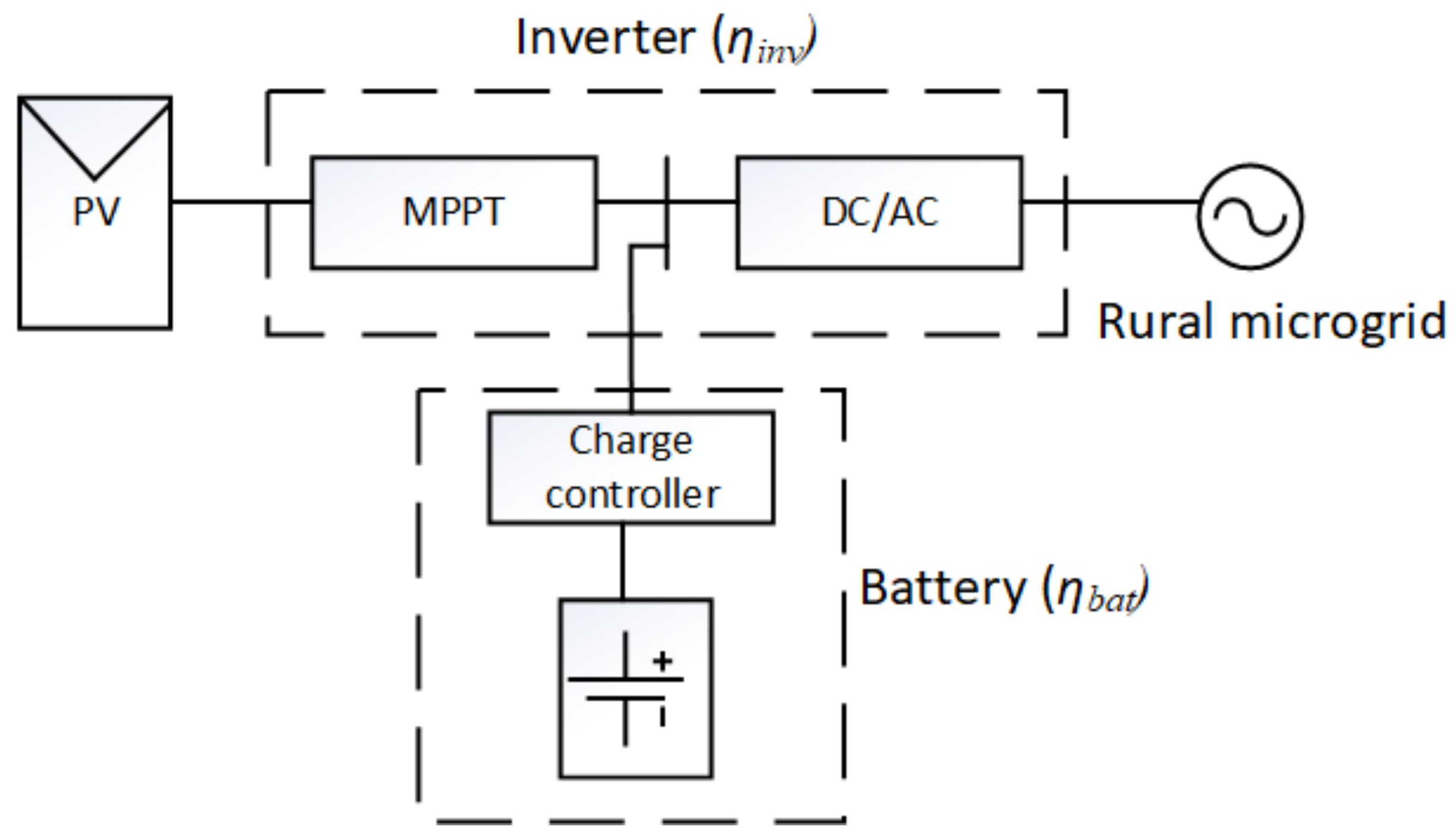
Central PV System Design
6. Conclusions
Author Contributions
Funding
Acknowledgments
Conflicts of Interest
References
- World Bank. Sustainable Energy for All Database. Available online: https://data.worldbank.org/indicator/EG.ELC.ACCS.ZS (accessed on 31 July 2018).
- Forbes. Available online: https://www.forbes.com/sites/suparnadutt/2018/05/07/modi-announces-100-village-electrification-but-31-million-homes-are-still-in-the-dark/#2333f11b63ba (accessed on 31 July 2018).
- Sastry, E.V.R. Village electrification programme in India. In Proceedings of the 3rd World Conference on Photovoltaic Energy Conversion, Osaka, Japan, 11–18 May 2003; pp. 2125–2128. [Google Scholar]
- Hubble, A.H.; Ustun, T.S. Composition, placement, and economics of rural microgrids for ensuring sustainable development. Sustain. Energy Grid. Netw. 2018, 13, 1–18. [Google Scholar] [CrossRef]
- Theo, W.L.; Lim, J.S.; Ho, W.S.; Hashim, H.; Lee, C.T. Review of distributed generation (DG) system planning and optimisation techniques: Comparison of numerical and mathematical modelling methods. Renew. Sustain. Energy Rev. 2017, 67, 531–573. [Google Scholar] [CrossRef]
- Diesendorf, M.; Elliston, B. The feasibility of 100% renewable electricity systems: A response to critics. Renew. Sustain. Energy Rev. 2018, 93, 318–330. [Google Scholar] [CrossRef]
- Jiang, T.; Costa, L.; Tordjman, P.; Venkata, S.S.; Siebert, N.; Kumar, J.; Puttgen, H.B.; Venkataraman, A.; Dutta, S.; Li, Y.; et al. A microgrid test bed in Singapore: An electrification project for affordable access to electricity with optimal asset management. IEEE Electrif. Mag. 2017, 5, 74–82. [Google Scholar] [CrossRef]
- Planas, E.; Andreu, J.; Gárate, J.I.; de Alegría, I.M.; Ibarra, E. AC and DC technology in microgrids: A review. Renew. Sustain. Energy Rev. 2015, 43, 726–749. [Google Scholar] [CrossRef]
- Jordehi, A.R. Allocation of distributed generation units in electric power systems: A review. Renew. Sustain. Energy Rev. 2016, 56, 893–905. [Google Scholar] [CrossRef]
- Abdmouleh, Z.; Gastli, A.; Ben-Brahim, L.; Haouari, M.; Al-Emadi, N.A. Review of optimization techniques applied for the integration of distributed generation from renewable energy sources. Renew. Energy 2017, 113, 266–280. [Google Scholar] [CrossRef]
- Hilton, G.; Cruden, A.; Kent, J. Comparative analysis of domestic and feeder connected batteries for low voltage networks with high photovoltaic penetration. J. Energy Storage 2017, 13, 334–343. [Google Scholar] [CrossRef]
- Aman, M.M.; Jasmon, G.B.; Bakar, A.H.A.; Mokhlis, H. A new approach for optimum simultaneous multi-DG distributed generation Units placement and sizing based on maximization of system loadability using HPSO (hybrid particle swarm optimization) algorithm. Energy 2014, 66, 202–215. [Google Scholar] [CrossRef]
- Kefayat, M.; Ara, A.L.; Niaki, S.N. A hybrid of ant colony optimization and artificial bee colony algorithm for probabilistic optimal placement and sizing of distributed energy resources. Energy Convers. Manag. 2015, 99, 149–161. [Google Scholar] [CrossRef]
- Adefarati, T.; Bansal, R.C. Integration of renewable distributed generators into the distribution system: A review. IET Renew. Power Gener. 2016, 10, 873–884. [Google Scholar] [CrossRef]
- Prakash, P.; Khatod, D.K. Optimal sizing and siting techniques for distributed generation in distribution systems: A review. Renew. Sustain. Energy Rev. 2016, 57, 111–130. [Google Scholar] [CrossRef]
- Asmuth, P.; Verstege, J.F. Optimal network structure for distribution systems with microgrids. In Proceedings of the 2005 International Conference on Future Power Systems, Amsterdam, The Netherlands, 16–18 November 2005. [Google Scholar] [CrossRef]
- Willis, H.L. Power Distribution Planning Reference Book, 2nd ed.; Marcel Dikker: New York, NY, USA, 2004. [Google Scholar]
- Pabla, A.S. Electric Power Distribution, 6th ed.; Tata McGraw-Hill Education: New Delhi, India, 2012. [Google Scholar]
- Gouin, V.; Alvarez-Hérault, M.C.; Raison, B. Optimal planning of urban distribution network considering its topology. In Proceedings of the 23nd International Conference on Electricity Distribution, Lyon, France, 15–18 June 2015. [Google Scholar]
- Wolfram Mathworld. Available online: http://mathworld.wolfram.com/SimulatedAnnealing.html (accessed on 31 July 2018).
- Das, J.C. Power System Analysis: Short-Circuit Load Flow and Harmonics, 2nd ed.; CRC Press: Boca Raton, FL, USA, 2016. [Google Scholar]
- MATPOWER. Available online: http://www.pserc.cornell.edu/matpower/ (accessed on 31 July 2018).
- Islam, M.; Mekhilef, S.; Hasan, M. Single phase transformerless inverter topologies for grid-tied photovoltaic system: A review. Renew. Sustain. Energy Rev. 2015, 45, 69–86. [Google Scholar] [CrossRef]
- The Satellite Application Facility on Climate Monitoring. Available online: http://www.cmsaf.eu/EN/Home/home_node.html (accessed on 31 July 2018).
- PVGIS Version 5 Release Candidate. Available online: http://re.jrc.ec.europa.eu/PVGIS5-beta.html (accessed on 31 July 2018).
- Pillai, G.; Naser, H.A.Y. Techno-economic potential of largescale photovoltaics in Bahrain. Sustain. Energy Technol. Assess. 2018, 27, 40–45. [Google Scholar] [CrossRef]
- Georgitsioti, T. Photovoltaic Potential and Performance Evaluation Studies in India and the UK. Ph.D. Thesis, Northumbria University, Tyne and Wear, UK, November 2015. [Google Scholar]


| From | To | Distance (m) | R (in p.u.) | X (in p.u.) |
|---|---|---|---|---|
| 1 | 2 | 11 | 0.013 | 0.011 |
| 2 | 3 | 11 | 0.013 | 0.011 |
| 3 | 4 | 12 | 0.015 | 0.012 |
| 3 | 5 | 78 | 0.095 | 0.076 |
| 5 | 6 | 78 | 0.095 | 0.076 |
| 6 | 7 | 59 | 0.072 | 0.057 |
| 7 | 8 | 42 | 0.051 | 0.041 |
| 8 | 9 | 12 | 0.015 | 0.012 |
| 9 | 10 | 31 | 0.038 | 0.030 |
| 10 | 11 | 31 | 0.038 | 0.030 |
| 10 | 12 | 77 | 0.094 | 0.075 |
| 12 | 13 | 94 | 0.115 | 0.091 |
| 13 | 14 | 17 | 0.021 | 0.016 |
| 14 | 15 | 56 | 0.068 | 0.054 |
| 15 | 16 | 26 | 0.032 | 0.025 |
| 16 | 17 | 13 | 0.016 | 0.013 |
| 17 | 18 | 38 | 0.046 | 0.037 |
| 15 | 19 | 39 | 0.048 | 0.038 |
| 15 | 20 | 35 | 0.043 | 0.034 |
| 20 | 21 | 20 | 0.024 | 0.019 |
| 21 | 22 | 19 | 0.023 | 0.018 |
| 22 | 23 | 19 | 0.023 | 0.018 |
| 21 | 24 | 27 | 0.033 | 0.026 |
| 13 | 25 | 59 | 0.072 | 0.057 |
| 13 | 26 | 83 | 0.101 | 0.080 |
| 26 | 27 | 14 | 0.017 | 0.014 |
| 27 | 28 | 56 | 0.068 | 0.054 |
| 28 | 29 | 63 | 0.077 | 0.061 |
| Load | No. of Units | Wattage | Coverage (fraction) | Connected Load (W) | No. of Households | Total |
|---|---|---|---|---|---|---|
| Domestic Lighting | 3 | 11 | 1 | 33 | 29 | 957 |
| Street Lights | 1 | 11 | 0.5 | 5.5 | 29 | 159.5 |
| Fans | 1 | 40 | 0.5 | 20 | 29 | 580 |
| Refrigeration | 1 | 100 | - | 100 | 29 | 100 |
| Television | 1 | 80 | 0.4 | 32 | 29 | 928 |
| Radio | 1 | 5 | 0.4 | 1.75 | 29 | 58 |
| Other Loads | 1 | 100 | 0.1 | 10 | 29 | 290 |
| Parameter | Value |
|---|---|
| PV module technology | Monocrystalline Silicon |
| Manufacturer and model | Ecosol PV tech Mono 75 Wp 36 cells |
| No. of PV modules in series | 4 |
| No. of parallel strings | 33 |
| Array nominal (STC) power | 9.9 kWp |
| MPPT converter maximum and European efficiencies | 97%/95% |
| Battery technology | Lead acid |
| Battery bank voltage | 48 V |
| Nominal capacity | 7200 Ah |
| Number of units | 24 in series × 8 in parallel |
© 2018 by the authors. Licensee MDPI, Basel, Switzerland. This article is an open access article distributed under the terms and conditions of the Creative Commons Attribution (CC BY) license (http://creativecommons.org/licenses/by/4.0/).
Share and Cite
Mothilal Bhagavathy, S.; Pillai, G. PV Microgrid Design for Rural Electrification. Designs 2018, 2, 33. https://doi.org/10.3390/designs2030033
Mothilal Bhagavathy S, Pillai G. PV Microgrid Design for Rural Electrification. Designs. 2018; 2(3):33. https://doi.org/10.3390/designs2030033
Chicago/Turabian StyleMothilal Bhagavathy, Sivapriya, and Gobind Pillai. 2018. "PV Microgrid Design for Rural Electrification" Designs 2, no. 3: 33. https://doi.org/10.3390/designs2030033
APA StyleMothilal Bhagavathy, S., & Pillai, G. (2018). PV Microgrid Design for Rural Electrification. Designs, 2(3), 33. https://doi.org/10.3390/designs2030033