
Article

A Frequency–Stress–Ratio Fatigue Index for Polymer Composites
by
Jose Luis Valencia-Sanchez
1,†,
Ciro A. Rodríguez-González
2,
Ulises Figueroa-López
3,
Alvaro Frutos
4,
Jose Guadalupe Rangel-Ramirez
1 and
Moises Jimenez-Martinez
1,*,†
1
School of Engineering and Science, Tecnologico de Monterrey, Via Atlixcayotl 5718, Puebla 72453, Puebla, Mexico
2
School of Engineering and Sciences, Tecnologico de Monterrey, Av. Eugenio Garza Sada Sur 2501, Col. Tecnologico, Monterrey 64849, Nuevo León, Mexico
3
School of Engineering and Sciences, Tecnologico de Monterrey, Av. Lago de Guadalupe Km 3.5, Margarita Maza de Juárez, Ciudad Lopez Mateos 52926, Estado de México, Mexico
4
Kautex Textron de Mexico, S. de R.L. de C.V., Autop. México-Puebla 117, Sanctorum, Heroica Puebla de Zaragoza 72761, Puebla, Mexico
*
Author to whom correspondence should be addressed.
These authors contributed equally to this work.
Designs 2026, 10(3), 63; https://doi.org/10.3390/designs10030063
Submission received: 9 April 2026 / Revised: 27 May 2026 / Accepted: 1 June 2026 / Published: 4 June 2026
(This article belongs to the Section Mechanical Engineering Design)

Abstract

Composite materials, known for their enhanced mechanical strength through fiber reinforcement, are increasingly used in industrial applications. However, like metals, they suffer strength degradation from cyclic loading, making fatigue failure a critical concern. The fatigue behavior of polymer composites is strongly influenced by factors such as stress amplitude, stress ratio, and loading frequency. Conventional stress-life approaches often treat these factors independently, which limits their predictive accuracy. This study introduces a novel frequency–stress–ratio fatigue index, integrated into a residual-strength degradation approach, to predict fatigue life under constant amplitude, tension-tension loading conditions. To the best of the authors’ knowledge, the majority of models available in the literature require substantial experimental data to calibrate the parameters essential for their application in real-world scenarios. The proposed model requires only two material parameters and assumes failure occurs when the residual strength degrades to the level of the applied maximum stress. The results demonstrate that the proposed formulation provides a unified representation of fatigue behavior influenced by both cycle-dominated and time-dependent mechanisms, offering robust predictive capabilities. This approach not only addresses a critical need for reliable and practical fatigue prediction methods in composite materials but also contributes significantly to the optimization of engineering design processes.

1. Introduction

Polymer matrix composites are increasingly employed in structural applications where cyclic loading governs service life. In such contexts, fatigue behavior is strongly influenced by the combined effects of stress amplitude, stress ratio, and loading frequency, particularly due to the viscoelastic nature of polymer matrices. Classical fatigue approaches, most notably stress–life (S–N) formulations, have proven effective for metallic materials but remain limited in their ability to consistently account for time-dependent damage mechanisms and stress ratio effects in polymer composites. Several extensions to traditional fatigue models have been proposed to address these limitations, including residual strength degradation frameworks, energy-based damage indicators, and empirical stress ratio corrections. While these approaches have improved predictive capability, they often treat stress ratio and frequency as independent modifiers or require many fitting parameters, limiting their robustness when experimental data are sparse. Moreover, the physical interpretation of frequency effects is frequently obscured, despite experimental evidence linking fatigue damage in polymers to viscoelastic dissipation and self-heating phenomena.
The frequency–stress–ratio (FSR) index unifies stress amplitude, stress ratio, and loading frequency into a single scalar quantity, embedded within a residual strength degradation framework for predicting fatigue life under constant-amplitude loading. Designed for simplicity, the formulation requires only two material parameters, focusing exclusively on tension–tension, constant-amplitude fatigue loading of conventionally manufactured laminated polymer composites. Scenarios involving negative stress ratios, variable-amplitude loading, or architecturally heterogeneous materials fall outside the model’s scope. The proposed framework is validated using independent experimental datasets from the literature, with its predictive capability assessed through cross-validation, uncertainty quantification, and parameter identifiability analysis. This study introduces the FSR index as a compact descriptor of fatigue severity, offering a practical tool for fatigue-life prediction in polymer composites, particularly when data availability is limited.

2. Fatigue Life Models for Composite Materials

Fatigue life prediction models for polymer composites are classified based on their theoretical foundation, methodological approach, and the scale of damage assessment. Broadly, modern classifications distinguish between empirical and phenomenological models, such as stress-life (S–N) and strain-life ( ϵ –N), which fit curves to experimental data for high-cycle and low-cycle fatigue, respectively [1,2,3]. These are complemented by physics-based and thermodynamic models, which incorporate principles like unified mechanics theory and entropy-based frameworks to account for energy dissipation, entropy generation, and damage evolution without relying on detailed loading histories [4].
More recently, machine learning and data-driven methods—including artificial neural networks, random forest algorithms, and physics-informed neural networks—have emerged, offering advanced pattern recognition and predictive capabilities for complex composite behaviors [2,5]. These models are further categorized by the damage scale they address. Macroscopic approaches use classical laminate theory to predict bulk behavior, mesoscopic models analyze periodic features at the unit cell level using representative volume elements (RVE), and microscopic models, such as micromechanics of fatigue (MMF), focus on stress distributions within fibers, the matrix, and their interfaces [1,6].
This multi-scale, multi-method taxonomy highlights the diversity of strategies available for fatigue life prediction in polymer composites, reflecting significant advances in both materials science and computational technologies.
Phenomenological models remain valid in composite fatigue analysis because they directly utilize macro-level properties, such as S–N curves, stiffness and strength degradation, and constant life diagrams, to represent complex fatigue behavior without requiring detailed microstructural modeling [7,8]. Widely used laminate fatigue models, including direct and stepwise fatigue damage models (FDMs), residual-strength models, and critical-plane approaches, are phenomenological in nature and are readily integrated into finite element codes for engineering applications [8,9]. These models efficiently reduce the need for extensive testing by enabling accurate predictions with just a few unidirectional S–N curves, allowing extrapolation to arbitrary laminate configurations [8]. Methods like time–temperature superposition further streamline testing, permitting accelerated construction of fatigue master curves and environmental lifetime estimates [7]. Basically, these modeling approaches are aligned with industry standards and Basquin and Coffin–Manson parameters, and constant life diagrams. This alignment streamlines their integration into design codes and reliability assessments for diverse structural applications, such as wind turbine blades, aircraft parts, and dental materials [10,11,12,13].

2.1. Influence of Stress Ratio on Fatigue Behavior of Some Polymer Composites

Fatigue-life prediction models for polymer composites consistently incorporate stress ratio parameters to address the necessity for calibration across varying loading conditions [14]. The stress ratio substantially influences fatigue behavior, with research demonstrating that moderate ratios ( R = 0.5 ) yield uniform damage distribution and stable surface temperatures, while lower ratios ( R = 0.1 ) lead to concentrated damage, localized heating, and earlier material failure [15]. At R = 0.5 , cyclic creep facilitates fiber realignment, temporarily increasing fatigue stiffness until offset by damage accumulation, whereas at lower ratios, damage growth dominates, resulting in increased energy dissipation per cycle and a continuously expanding hysteresis loop area [15,16]. Higher stress ratios, approaching unity, accelerate fatigue damage due to reduced relief during loading, resulting in faster crack growth rates and more rapid degradation of residual strength and stiffness [14]. The dominant damage mechanisms also shift to matrix cracking and fiber breakage, which are more prevalent at higher ratios, while delamination and interfacial debonding are significant at lower ratios. Finite element simulations further reveal that stress ratio affects the distribution of Von Mises stress, with the matrix playing a crucial role in load transfer and fiber alignment [17]. Consequently, composites subjected to lower stress ratios may retain greater residual strength after cycling, while higher ratios exacerbate environmental sensitivities, such as temperature and moisture, intensifying fatigue damage [18].

2.2. Dissipated Power and Energy-Based Approaches for Analyzing Cyclic Fatigue in Viscoelastic Polymer Composites

The paradox in polymer composites, where identical amounts of dissipated energy produce varying effects depending on the time or rate of application, is a well-documented phenomenon in materials science. This behavior is primarily attributed to the viscoelastic nature of the polymer matrix. Although the total dissipated energy remains constant, its rate of dissipation influences the material’s failure mechanism—shifting it from ductile to brittle—and alters the energy distribution between thermal degradation and mechanical damage [19,20,21]. In the context of cyclic fatigue in viscoelastic polymer composites, dissipated power as an energy rate indicator frequently provides a more accurate representation of material behavior than total dissipated energy. This distinction arises from the next considerations described as follows.
Polymers are highly viscoelastic and sensitive to strain rate, with fatigue strength affected by loading frequency and self-heating [22,23]. Changes in frequency alter power dissipation, which is more relevant to damage than total energy per cycle, as temperature rise and thermal degradation depend on power [22,23,24]. Dynamic fatigue tests show surface temperature plateaus when heat convection balances dissipated energy, and power-law relationships link strain amplitude, energy density, and temperature increase [23], connecting power to thermal–mechanical degradation.
Self-heating effects on polymers reveal that fatigue life is influenced not only by the mechanical work applied but also by the rate at which this work is converted into heat and the resulting temperature distribution within the material [22,23]. Studies on short-fiber reinforced polymers highlight the critical role of energy dissipation and heat release in assessing material damage. The fraction of mechanical work converted into heat profoundly influences fatigue life, driven by microstructural interactions and interfacial dynamics [25]. Accordingly, a power-based parameter, which directly reflects the rate of heat generation, provides a more accurate representation of the coupled thermo-mechanical state than traditional measures based solely on cumulative energy, as it accounts for the critical influence of temporal effects.
Energy-based fatigue indicators, such as dissipated energy per cycle or over the lifespan, have proven effective but are also highly sensitive to loading conditions, stress ratios, and creep effects [15,22,24,26,27]. In viscoelastic materials, damage progression typically occurs in three distinct stages: initial softening, a quasi-steady phase, and accelerated degradation. This evolution can be effectively monitored through the dissipated energy per cycle [22,27]. These phases align with changes in the rate of energy dissipation and self-heating. A power-based indicator provides a more effective distinction between regimes: one where cyclic viscoelastic dissipation dominates, characterized by moderate power and stable temperature, and another governed by cyclic creep and thermal instability, marked by a rapid increase in both power and temperature [15,23,24,26,27].
Previous research suggests that energy dissipation-based descriptors, closely linked to heat generation and creep development, play a key role in facilitating damage assessment and life prediction for short fiber reinforced plastics (SFRPs) and laminates [15,23,25,26,27]. Recent life-prediction models for viscoelastic polymers and composites integrate dissipation and cyclic-creep interaction as key variables. These models establish a direct link between energy dissipation, temperature, and the time-dependent properties of these materials [15,24,26,27]. Given that creep and temperature effects are fundamentally rate-controlled, defining the fatigue indicator in terms of dissipated power—rather than accumulated energy—provides better alignment with time-temperature superposition principles, cyclic-creep interaction models, and damage-entropy or heat-based criteria for composite laminates [1,15,23,24,25,26,27].

2.3. An Indicator Based on Stress Ratio R, Frequency f, and Stress σ

For viscoelastic polymer composites subjected to cyclic loading, adopting a dissipated power perspective facilitates the development of phenomenological damage indicators that integrate frequency, stress level, and stress ratio. Fatigue life is primarily governed by the rate at which mechanical work is transformed into irreversible energy—such as viscous/creep and plastic dissipation—and heat. Energy-based models consistently demonstrate that damage correlates with the dissipated energy per cycle and its rate, which is jointly influenced by stress amplitude, stress ratio, and loading frequency [7,22,23,24,26].
Within the framework of linear viscoelasticity, the energy dissipated per unit volume during a cycle ( W d i s s ) is considered as a function of time [28].
W d i s s = σ d ϵ = 0 T σ ( t ) d ϵ ( t ) d t d t
In dynamic analysis involving cyclic loading, the frequency f is commonly expressed in terms of angular velocity ω = 2 π f . Accordingly, the strain rate ( ϵ ˙ ) is defined relative to a reference strain ϵ 0 as
ϵ ˙ = d ϵ ( t ) d t = ω ϵ 0 c o s ( ω t )
According to the principles of linear viscoelastic mechanics, the material response under sinusoidal load can be characterized by a complex modulus E * that accounts for both elastic and viscous effects, represented respectively by the loss modulus ( E ) and storage modulus ( E ).
E * = E ( ω ) + E ( ω )
Consequently, the stress ( σ ) as a function of this complex ( E * ) is formulated as
σ ( t ) = ϵ 0 [ E sin ( ω t ) + E cos ( ω t ) ]
The resultant dissipated energy is derived by the integration
W d i s s = π E ϵ 0 2
Considering that η e f f is an effective (temperature- and rate-dependent) viscosity encoded as E″ = η e f f ω in loss modulus or viscoelastic parameters [7,23,24,26] the dissipated power per unit volume is schematically represented for further analysis as
( P d i s s = W d i s s · f ) f , η e f f , σ ( ϵ 0 )
This relationship underscores the pivotal role of frequency and applied stress—via strain amplitude—in governing the rate of energy dissipation and, consequently, the rate of fatigue damage accumulation.
Experiments on polymers and short fiber-reinforced polymers (SFRPs) demonstrate that, at a fixed stress level, higher frequencies lead to increased dissipated power and self-heating. Additionally, variations in the stress ratio R alter the balance between cyclic and creep components, thereby influencing the total dissipated energy [7,22,24,25,26]. Because fatigue damage in such materials is driven by the rate of dissipated energy or related entropy measures, and this rate scales with both f and a nonlinear function of σ and R, it is natural to define phenomenological scalars that compress these dependencies.
Recent work explicitly constructs shift factors in dissipated energy-based life models that depend on stress ratio and temperature, applied to viscoelastic adhesives [26]. Reviews highlight that most practical models are, in fact, phenomenological fits of macro-properties to combinations of stress, stress ratio, frequency and temperature [7]. Within this context, it can be assumed that a frequency over applied stress quotient f σ a could influence the damage per cycle, which is directly related to viscoelastic heating and mechanical work in tension-tension fatigue. According to this, the damage per cycle can be driven by viscoelastic energy dissipation in that mechanical work is converted into heat rather than purely mechanical crack growth. A damage indicator D e n is proposed as a compact descriptor of fatigue severity:
D e n ( f σ ) ( R )
Considering that the base quotient f σ represents dynamic loading severity per unit stress, reflecting that increasing f at fixed σ raises the power input rate and thus accelerates damage, while increasing σ at fixed f changes both local overstress and creep-like contributions [22,23,25]. The exponent (R) allows the stress ratio to modulate how sensitively damage responds to that dynamic severity. Energy-based and creep-enhanced fatigue models show that as R increases (approaching tension–tension creep-dominated regimes), the relative weight of time-dependent viscous/creep dissipation grows and the link between stress level and damage becomes strongly nonlinear [7,22,25,26]. A stress ratio dependent exponent therefore captures the experimentally observed nonlinear influence of R on life and damage, beyond a simple linear mean stress correction. Thus, while D p h e n is not derived from first principles, it is consistent with dissipated power scaling with frequency and stress, with the known role of viscosity/creep and stress ratio in viscoelastic fatigue, and with current phenomenological, energy-based life prediction approaches for polymers and polymer composites [7,22,23,24,25,26].
Applying the stress ratio R as an exponent to the quotient ( f σ ) R fundamentally shifts the model to a nonlinear interaction model approach. In the physics of polymer composites, this suggests that the material’s sensitivity to viscous effects is not constant but is instead modulated by the mean stress level [29]. The impact of the loading rate ( f / σ ) on the damage accumulation rate is nonlinearly dependent on the stress ratio. The formulation ( f / S ) R treats the stress ratio R as a sensitivity exponent, modulating the material’s response to viscous dissipation. This approach is consistent with the observed transition from cycle-dependent damage at low R values to time-dependent (creep-dominant) failure at high R values, effectively capturing the shift in the matrix’s free volume and molecular mobility under sustained mean loads [30,31,32]. Consequently, the proposed expression provides a phenomenological means of capturing changes in molecular mobility and free-volume evolution within the polymer matrix under sustained mean loading.
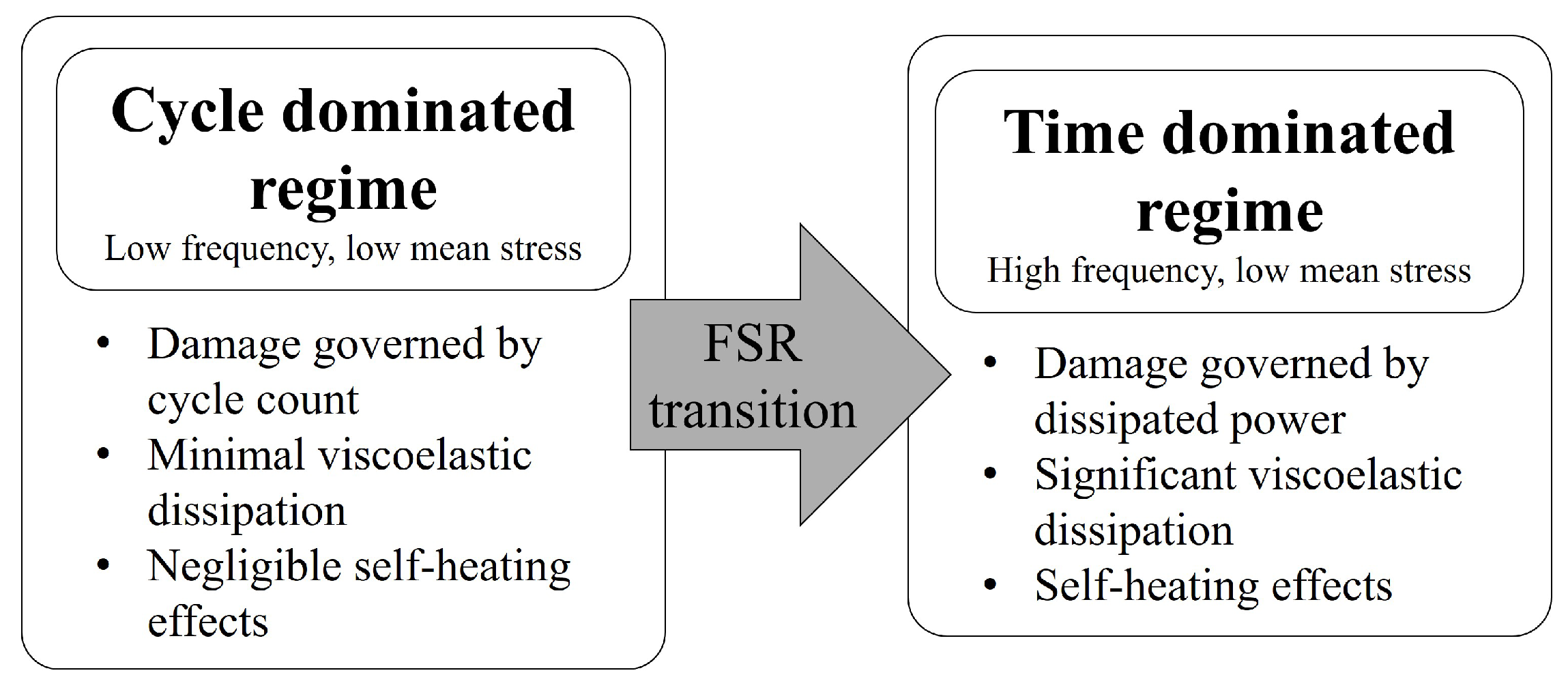
Conceptually, fatigue behavior under cyclic loading can be divided into the following two regimes:
  • Cycle-Dominated Regime: Initially, fatigue damage is primarily governed by stress amplitude and cycle count. Frequency effects are minimal, and damage accumulation scales predominantly with the number of load reversals. This regime is typically observed at low frequencies and low mean stresses, where viscoelastic dissipation per cycle is limited.
  • Time-Dominated Regime: As conditions change, fatigue degradation becomes strongly influenced by viscoelastic dissipation and self-heating. In this regime, damage accumulation depends on the rate of energy dissipation per unit time, rather than on cycle count alone. This regime dominates at higher frequencies and higher mean stresses.
The transition between these two regimes is continuous, not discrete, and is modulated by the combined effects of stress ratio and loading frequency. To describe this transition, the frequency–stress–ratio (FSR) index is used as a compact phenomenological descriptor. The FSR index incorporates frequency, weighted by a stress ratio-dependent exponent, to bridge the cycle- and time-dominated regimes.
The conceptual role of the F S R index in linking these fatigue regimes is illustrated schematically in Figure 1.
By considering the ratio f σ , a model effectively balances the mechanical loading severity with the rate at which the load is applied. If this parameter is high, it suggests that the stress fluctuations are mild (high R), cycling is slow (low frequency), or both. Under these conditions, the damage per cycle is relatively small, and the predicted fatigue life is longer. Conversely, if the effective parameter is low, it shows severe stress fluctuations (low R), a high cycling rate (high frequency), or both—conditions that are known to accelerate damage accumulation and thus shorten fatigue life. As an example, this behavior could be modeled by a power function,
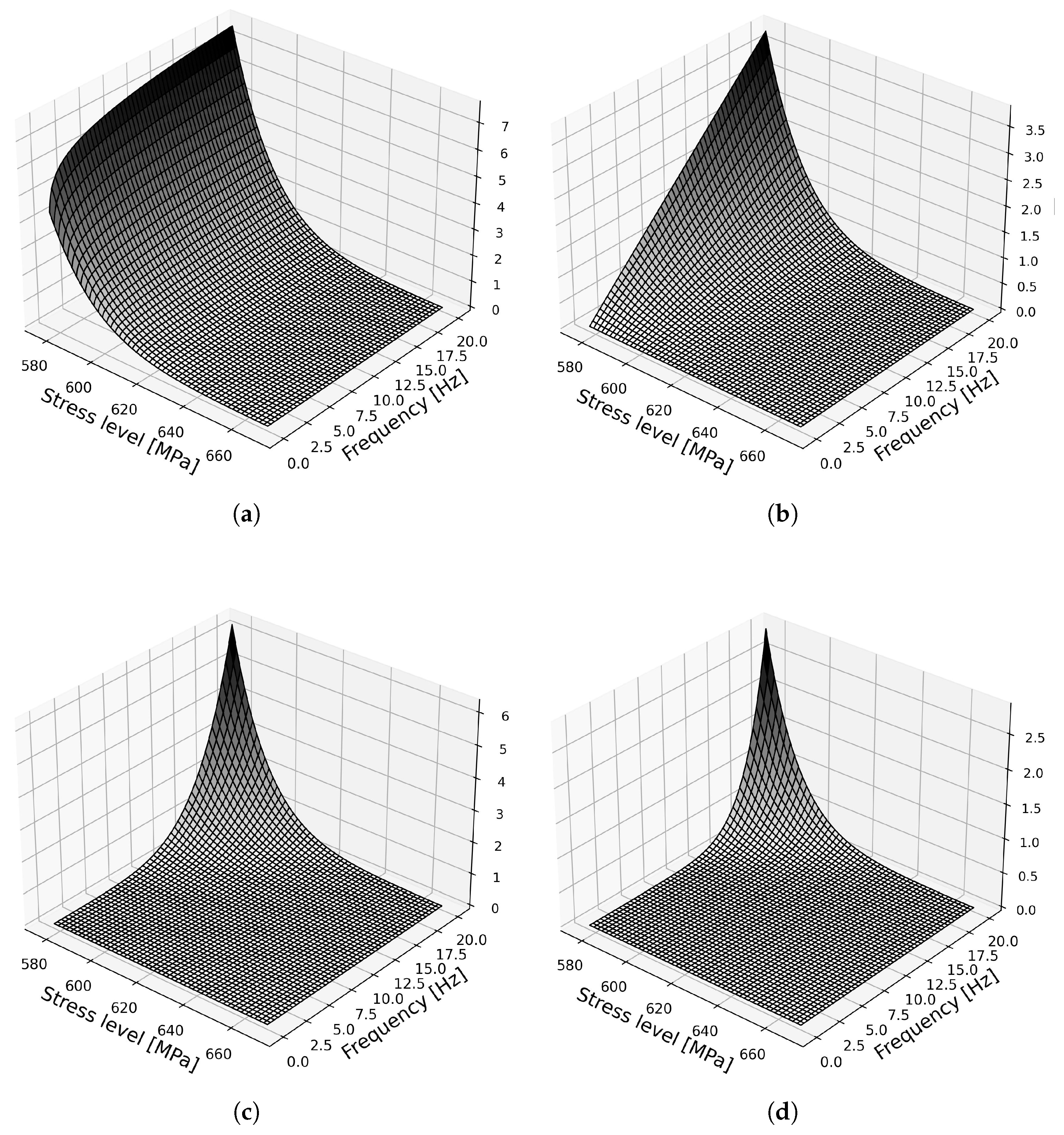
D = σ 0 ( f σ ) ( R )
where D could correspond to damage, σ 0 is the static strength, σ is the applied stress, f is the frequency and R is the stress ratio. In Figure 2 the relationship between these parameters can be observed.
Soft fluctuations in the stress ratio R led to slower damage accumulation and longer fatigue life, especially under tensile loading with both positive maximum and minimum stresses, when R falls between 0 and 1 (Figure 3). However, when R exhibits negative values (when load reversals are applied, such as alternating tension and compression), the situation becomes more complex. Negative values of R indicate that the loading cycle involves a reversal. For example, fully reversed loading where R = 1 . In such cases, the damage mechanisms may not be directly comparable to those under purely tensile conditions. Compressive stresses can trigger different microstructural responses, such as buckling, localized damage, or different crack initiation modes [33], than tensile stresses. For positive R, a value closer to 1 means that the minimum stress is nearly equal to the maximum stress, so the load fluctuation is small. For instance, an R of 0.5 does not necessarily imply a milder loading in the same way that R = 0.8 does in tension. Fatigue models dealing with negative R often use additional parameters, the mean stress, or amplitude of stress, to more accurately characterize the severity of the cycle. Table 1 provides a comprehensive summary of the key variables associated with the fatigue ratio.
To consider stress ratio R as a creep-fatigue weighting factor of the quotient f / σ , it is assumed that two failure mechanisms are present in tensile-tensile tests. One corresponds to fatigue damage cyclic dependent. The other corresponds to creep as damage related to fluency that appears when a load is maintained over time periods. Under this condition, it is considered that the stress ratio R shows which mechanism rules theoretically. When the exponent R of the term f / σ is close to 0, the influence of frequency decreases, allowing stresses to be the mean predictor. It is a pure fatigue case where damage is related to the applied number of cycles and is time-independent. In other cases, when R approaches 1, it is assumed to be an almost static condition such as creep. The frequency considered as the inverse of loading time is relevant, enabling the term f / σ as a predictor of creep rupture. Using R as an exponent is justified as a transition predictor adapting the prediction equation from a pure fatigue model to a creep model.
It could be generalized that the models that include the term “ ( 1 R ) ” are preferably applicable to tension-load conditions if other criteria are not referred to include compression-load conditions. Burhan and Ho [34] report for the D’Amore et al. [35], Epaarachchi [36] and Poursartip [37] models a poor or reasonable capability for curve fitting and applicability to different stress ratios when comparing them taking negative R values.
The FSR term is introduced as a phenomenological representation of the rate-dependent viscoelastic dissipation that governs fatigue degradation in polymer matrix composites. Under cyclic loading, the polymer matrix exhibits a phase-lagged stress–strain response, and the associated energy loss per cycle W d increases with both frequency and the amplitude of the viscoelastic strain component [38,39,40]. Although the present formulation does not explicitly compute W d , G ( ω ) , or the full relaxation spectrum, the FSR index is constructed to reflect the combined influence of frequency, stress amplitude, and mean stress on the effective dissipated power. In this context, the ratio f / σ serves as a compact surrogate for the rate at which dissipative mechanisms are activated. Higher frequencies increase the number of viscoelastic loading–unloading cycles per unit time, while higher stresses reduce the relative contribution of viscous deformation to the total strain [41,42]. The exponent R modulates this balance by incorporating the effect of mean stress, which elevates the sustained viscoelastic strain and shifts the material response toward creep-like dissipation. Although R is not a mechanistic parameter in the strict constitutive sense, its role in the FSR term reflects the well-established observation that higher mean stresses accelerate viscoelastic damage accumulation [43].
Thus, the FSR index does not claim to be a direct measure of dissipated energy or a microstructural damage variable. Instead, it functions as a scalar proxy that captures the macroscopic consequences of viscoelastic dissipation on fatigue life. This approach is consistent with classical phenomenological fatigue models, where physically motivated but simplified descriptors are used to represent complex internal processes that cannot be directly measured from the available data [44,45]. By framing the FSR term as a phenomenological surrogate for dissipated power, the model remains aligned with the underlying physics of viscoelastic fatigue while acknowledging that its structure is calibrated from macroscopic S–N data rather than derived from first principles viscoelastic constitutive equations.

3. Materialsand Methods

3.1. Model Formulation

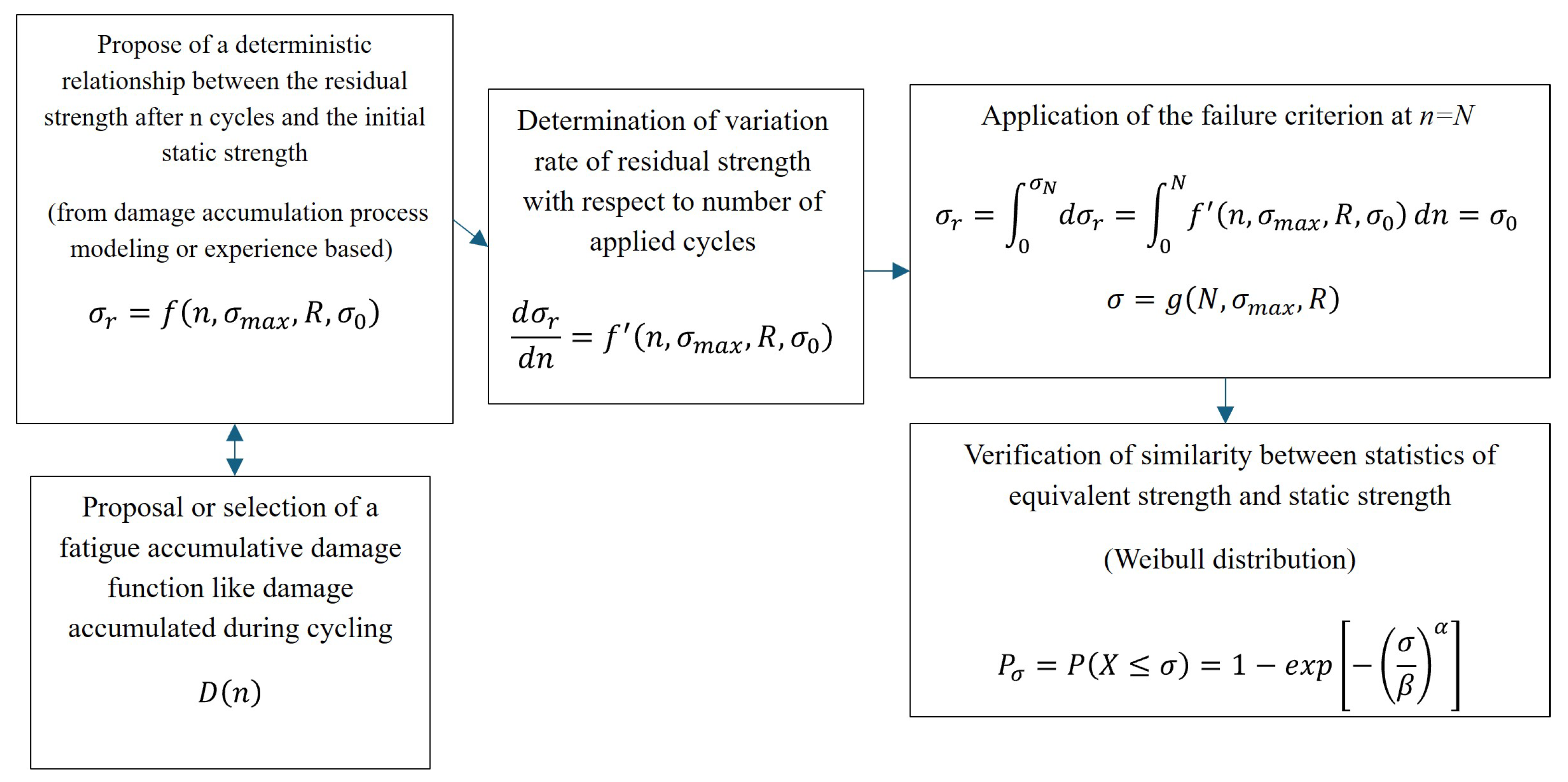
A guideline based on Sendeckyj [46] and D’Amore and Grassia [47] was proposed and used to derive an explicit equation to calculate the number of cycles to failure N under a given stress level σ , considering frequency (f), ultimate strength ( σ u ), and stress ratio (R). The guideline is presented in Figure 4.
It is assumed that the decay of the residual strength, σ n , depends on the number of applied cycles n. This named decay can be represented by a power law [48,49,50].
d σ n d n = a F n b
In Equation (9), σ n is the residual strength after n applied cycles; a and b are constants for the formulation. As a control parameter, a function F is proposed. This considers the properties of the material (in this case, static tensile strength σ 0 ), and parameters related to tests such as stress level σ m a x , the stress ratio R, and frequency f.
F = F ( R , σ 0 , σ m a x , f )
Assuming that fatigue life can be determined by integration of Equation (9), integration limits were defined by stating that materials fail when their residual strength reaches the maximum applied cyclic stress. After integration, the equation yields onto
σ r σ 0 = a F 1 b ( n 1 b 1 )
Considering the influence of the stress ratio and frequency on fatigue life of specimens, it is proposed a function F as follows:
F = c σ 0 ( σ m a x f ) R
By introducing function F in Equation (11), they following is obtained:
σ r σ 0 = σ 0 ( σ m a x f ) R 1 b ( n 1 b 1 )
Equivalences in Equations (14)–(16) were used to simplify the expression.
β = 1 b
α = 1 a c
δ = α β
When applying the specific condition σ m a x = σ r for n = N , the result is as follows:
σ m a x σ 0 = σ 0 ( σ m a x f ) R δ ( N β 1 )
Solving for N in Equation (17),
[ δ ( 1 σ m a x σ 0 ) ( f σ m a x ) R + 1 ] 1 β = N
The presented formulation is limited to tension–tension loading ( R 0 ); extending it to negative stress ratios would require additional damage mechanisms and is beyond the scope of this work. By normalizing frequency and stress using reference values, the FSR index achieves consistent results across different materials and test setups, eliminating unit dependence and enabling valid comparisons between datasets. The reference stress σ r e f f is chosen as the quasi-static ultimate tensile strength σ 0 in the same direction and laminate system as the fatigue data, aligning with the residual-strength approach where failure occurs when residual strength equals the maximum applied stress.
The reference frequency f r e f is set to 1 Hz, a standard in polymer and composite fatigue tests, where significant temperature increments are not expected, allowing one cycle per second normalization. Using the dimensionless form ( f f 0 ) / ( S S 0 ) does not alter the underlying physical rationale of the FSR term; rather, it makes the formulation mathematically rigorous and materially interpretable, which is essential for cross-dataset comparison [51,52,53]. Normalizing frequency and stress by reference values f 0 and S 0 eliminates hidden dimensionality in the raw f / S ratio and aligns the model with standard practice in fatigue and viscoelastic modeling, where dimensionless groups are preferred to avoid scale-dependent artifacts. This normalization also anchors the FSR term to material-specific physical scales, for example, f 0 = 1 Hz as a conventional fatigue frequency and S 0 = S u as the intrinsic strength scale, thereby improving interpretability without introducing new assumptions. The dimensionless form prevents dataset-specific frequency or stress magnitudes from artificially influencing parameter estimation, which enhances identifiability and ensures that the FSR term reflects relative loading severity rather than absolute test conditions. For these reasons, the normalized expression is the correct and more defensible representation of the same phenomenologically motivated surrogate for dissipated power.
Thus, the dimensionless severity index D ( R , F , σ ) is defined by Equation (19).
D = ( f f r e f σ m a x σ 0 ) R

3.2. Experimental Datasets

The datasets utilized in this study were sourced from published literature, including the works of Gao et al. [54], Hwang and Hang [55], Broutman and Sahu [56], and Yang and Liu [57]. These datasets encompass stress levels and the corresponding number of cycles to failure across various materials, frequencies, and stress ratios. The parameters required for the model were derived from this information. The reference designation assigned to these datasets and their associated parameters is “experimental data.”

3.3. Parameter Estimation

The fatigue life prediction model used in this study is defined by a nonlinear relationship, where the experimental variables number of cycles until failure ( N i ) and stress levels ( σ i ) are obtained from constant amplitude fatigue tests, and the material parameters δ and β must be determined. The model can be rearranged to an explicit form as in Equations (24) and (25), showing its nonlinear dependence on both parameters, which necessitates the use of a nonlinear regression procedure for parameter estimation. To facilitate stable convergence of the nonlinear solver, initial estimates for δ and β were derived from an approximate linearization; for sufficiently large values of N i , the model behaves in a nearly linear fashion between log ( N i ) and log ( σ i ) , allowing a simple least squares regression to provide preliminary values for δ and β . These initial guesses, δ 0 and β 0 , obtained from the slope and intercept of the linear fit, served as starting points for the subsequent nonlinear optimization. The parameters were then refined by minimizing the sum of squared residuals between the experimental data and the model prediction, with the minimization carried out using a Levenberg–Marquardt nonlinear least squares algorithm. This iterative method updates the parameter vector until convergence is achieved, ensuring that the final estimates δ and β offer the best fit to the experimental dataset in the least squares sense. After optimization, predicted values N p r e d were computed using the calibrated parameters. Residuals were analyzed to verify the absence of systematic trends, and the overall quality of the fit was assessed through the residual norm and visual inspection of the experimental versus predicted response. This procedure ensures a robust and reproducible determination of the fatigue model parameters.

3.4. Validation Strategy

The mean absolute error (MAE) is a metric that measures the average absolute difference between predicted values and actual outcomes [58,59], providing information on the typical size of prediction errors.
MAE = 1 n i = 1 n | y i y ^ i |
Equation (20) presents the MAE definition, where n, y i , and y ^ i correspond to the number of values, the real value and the predicted value. MAE designates the average absolute difference between predictions and actual outcomes; however, its raw value can be difficult to interpret when datasets have varying scales. Normalized mean absolute error (NMAE) addresses this issue by normalizing errors using a range of actual values, providing a scale-independent consistent basis for evaluating model accuracy across datasets [60,61]. In this case,
NMAE = MAE max ( y ) min ( y )
Root mean square error (RMSE) was the metric used to quantify the model’s prediction accuracy. The average RMSE across all iterations estimates model generalization to unseen data. It measures the average magnitude of the prediction error, providing a single value that reflects how close the model’s predicted values are to the observed values, applying
RMSE = 1 n i = 1 n ( y i y ^ 1 ) 2
where y i represents each observed value, y ^ i denotes the corresponding predicted value from the model, and n is the number of data points. It was considered that lower RMSE is evidence that the model predictions are closer to the actual observed results. As RMSE is sensitive to the scale of the target variable, its interpretation was contextualized with respect to the range and variability of that variable. A standard method is to normalize RMSE by dividing it by the difference between the maximum and minimum target values. Lower normalized RMSE values, approaching zero, indicate superior model performance [62]. In this context it is considered that RMSE values of 0.5 and 5.0 are comparably effective when the respective target ranges are 0 to 1 and 0 to 100.
NRMSE = RMSE value m a x value m i n
The robustness of the model was validated by applying the leave-one-out cross-validation (LOOCV) method. LOOCV is used in fatigue-related modeling to obtain reliable generalization estimates from small, expensive datasets, which is typical in composite fatigue testing. In LOOCV, a single data point is removed, the model is trained on the remaining data, and the omitted point is predicted [63]. This process was repeated for all data points to evaluate the model’s predictive performance on unseen data. Insight into how well the model and its provided parameters perform. Each LOOCV predicted value was an out-of-sample prediction because the corresponding data point was not used in the fitting process for that prediction. If the LOOCV predictions align closely with the observed data, the model is robust and not highly influenced by individual data points. This method assesses the sensitivity of the SN curve model to single observations, which is important when only one measurement per stress level is available. The approach is intended to provide confidence in the model’s accuracy even with a limited dataset [64]. In this process, NRMSE was used as the validation indicator for predictive error stability, with values closer to zero regarded as more robust.
To derive a lower tolerance limit (LTL) for the prediction model using bootstrapping, essentially it was calculated as a confidence bound on a quantile, considering that a prediction interval marks where the next single data point will likely fall, while a tolerance limit tells where a specified proportion of all future data points will fall, with a certain level of confidence [65]. In this context, a tolerance interval is a range within which a certain proportion (P) of the population is expected to fall, with a specified level of confidence ( γ ) [66,67]. In situations when mean ( μ ) and standard deviation ( σ ) are not known and must be estimated from a sample, bootstrapping can be applied [68]. It was considered that the dataset consists of single stress levels, each with one observed fatigue life, and the proposed model provides corresponding estimates. To evaluate model performance, a LOOCV approach is used, where each stress level is sequentially withheld, the model is retrained on the remaining levels, and a prediction is generated for the held-out level. Prediction error is then computed for each iteration. Bootstrapping is applied by resampling the residuals from the training folds with replacement; mean and deviation are re estimated for each bootstrap replicate, allowing predictive distributions to be generated for the held-out levels. Lower tolerance limits (LTLs) are computed as the percentile of bootstrap fractiles to ensure one-sided confidence. For performance metrics, the analysis includes RMSE on the log scale. It is assumed that in this way it is possible to add a lower tolerance limit to an S–N prediction polymer composite life curve obtained with single values for each experimental stress level. As only a single fatigue life or cycle to failure value per experimental stress level is known, the scatter at that level cannot be observed directly. For this case, the lower tolerance limits added come from the uncertainty in the fitted S-N curve parameters bootstrapping rather than from variability at that stress level per se [69]. In this work, the lower tolerance limit (LTL) is defined as a one-sided tolerance bound that covers 90% of the population with 95% confidence. In other words, the reported LTL corresponds to the stress (or life) level below which at most 10% of future specimens are expected to fall, with a 95% assurance level. This choice is consistent with common practice in structural design, where a 90/95 tolerance criterion is widely used as a conservative basis for allowable values [70,71,72]. The uncertainty in the LTL was quantified using a nonparametric case bootstrap applied at the specimen level for each dataset. For every dataset, we generated B = 2000 bootstrap resamples, refitted the model to each resample, and recomputed the corresponding LTL. The empirical distribution of these bootstrapped LTL values was then used to obtain the 95% confidence bound on the 90% population quantile. We deliberately used a case bootstrap rather than a residual bootstrap, because the residuals exhibit non-Gaussian behavior and mild heteroscedasticity, and the sample sizes are too small to justify strong parametric assumptions on the error structure [73]. This approach is statistically justified for such sparse data for two reasons. First, the tolerance bound is driven primarily by the between specimen variability, which is exactly what the case bootstrap resamples. Second, parametric tolerance interval formulas rely on distributional assumptions, such as normality and homoscedasticity of residuals, that are not well supported by the limited number of specimens in each dataset. The nonparametric case bootstrap therefore provides a conservative and assumption light estimate of the LTL and its uncertainty, which is more appropriate than relying on closed form parametric tolerance intervals under these data constraints.
Another assumption was that bootstrapping can be used also to address the variation between the S–N curve lower tolerance limit calculated using cycle scatter at each stress level and the S–N curve lower tolerance limit determined by assuming a mean number of cycles for each stress level based on a prediction model. This distribution accounts for variability that is not captured by predictions based solely on means, thereby quantifying the difference between an LTL derived from actual scatter and one assumed from a deterministic model. For sparse test points, resampling using either case or residual bootstrap techniques to preserve inherent material variability is used [74]. Each bootstrap replicate produces slight variations in regression slope, intercept, and residual standard deviation [75]. Calculating the lower tolerance limit (LTL) across this ensemble captures both model uncertainty and material scatter, enabling the generation of multiple S–N fits. Rather than yielding two distinct LTLs, true scatter versus mean only, this approach pretends to obtain a continuous distribution and a confidence band rather than a single curve. The median bootstrapped LTL typically could lie between these extremes, with percentile bounds serving to quantify the design margin.
The model is intentionally formulated to predict macroscopic load-carrying failure, not the onset or progression of early-stage damage. This choice is dictated directly by the nature of the available datasets, which report only the number of cycles to final fracture under constant-amplitude tension–tension loading. Because no intermediate measurements such as stiffness degradation, hysteresis evolution, temperature rise, or acoustic emission are provided, it is neither feasible nor scientifically defensible to construct or validate a model targeting micro-damage initiation or multi-stage damage evolution. The formulation is grounded in the role of viscoelastic energy dissipation as the dominant driver of fatigue degradation in polymer matrix composites. Under harmonic loading, the polymer matrix exhibits phase lagged deformation and rate dependent viscous flow, both of which contribute to cumulative energy loss and progressive strength reduction. The proposed FSR index serves as a compact surrogate for this rate dependent dissipative environment, integrating the combined effects of frequency, stress amplitude, and mean stress into a single scalar. However, while viscoelastic dissipation governs the rate of degradation, the model does not attempt to resolve the individual micro mechanisms—matrix microcracking, fiber–matrix debonding, or delamination—that may initiate long before final failure. These mechanisms are implicitly aggregated into the residual strength decay law, consistent with classical approaches in the literature. Given these constraints, the model’s scope is deliberately limited to predicting the cycle count at which the residual strength equals the applied maximum stress, which corresponds to the experimentally observable failure point in all datasets considered. Extending the model to earlier stage damage would require experimental observables that are not available in the present data and would necessitate a fundamentally different constitutive framework. For this reason, the model is not claimed to predict damage initiation, stiffness loss, or transitions between damage regimes, and any such interpretation would fall outside the intended and supportable scope of the work.

3.5. Identifiability and Uncertainty Analysis

The model was examined for structural and practical identifiability. By defining the composite loading function,
g ( σ , f , R ) = δ ( 1 σ σ u ) ( f σ ) R
where σ , σ u , f, and R correspond to applied stress, ultimate strength, frequency, and stress ratio, respectively. The model becomes as depicted in Equation (24):
N = ( δ g + 1 ) 1 β N β = δ g + 1 δ = N β 1 g
It follows that two sets of parameters ( δ , β ) can produce identical predictions for more than one value of g only if δ and β are equal. Thus, the model is structurally identifiable provided that the experimental matrix contains at least two distinct values of g. Practical identifiability was assessed via nonlinear regression, parameter-correlation analysis, and bootstrap resampling. The results show that a broad range of σ σ u is required to decorrelate δ and β ; when the stress range is narrow, the parameters become strongly correlated and their individual estimates are uncertain, even though the model predictions remain accurate. The ultimate strength σ u was fixed to avoid confounding with δ .
The formulation developed in this work is intended to predict macroscopic load carrying failure under constant amplitude tension–tension fatigue. The model assumes that failure occurs when the residual strength decays to the level of the applied maximum stress, consistent with classical residual strength approaches for polymer composites. Accordingly, the predicted fatigue life corresponds to the point at which the material can no longer sustain the imposed load, rather than to the onset of microstructural damage.
The model does not attempt to resolve individual damage mechanisms such as matrix microcracking, fiber–matrix debonding, delamination, or stiffness degradation. These processes may initiate well before final failure, but they are not explicitly represented in the present formulation. Instead, their cumulative effect is implicitly captured through the phenomenological degradation law governing the evolution of residual strength. As a result, the model provides a single stage description of damage accumulation and is not intended to identify transitions between early stage and late stage damage modes.
The scope of the model is further limited to R 0 loading conditions, where the assumption of monotonic tensile degradation remains physically meaningful. The formulation has not been validated for negative stress ratios, compression dominated cycles, or multiaxial loading, where additional mechanisms—such as fiber microbuckling or shear driven damage—become significant and would require an extended constitutive framework.
Within these boundaries, the model offers a compact and reliable means of predicting fatigue life based on macroscopic failure criteria. Its applicability to earlier stage damage evolution should be considered qualitative at best, and any interpretation beyond final load carrying failure lies outside the intended scope of the present work.

4. Results

4.1. Model Calibration Results

The model was applied to four different datasets, and its performance regarding the usage of different datasets is displayed in this part of the current section. All FSR index values are computed using the reference quantities defined in model formulation Section 2.1.
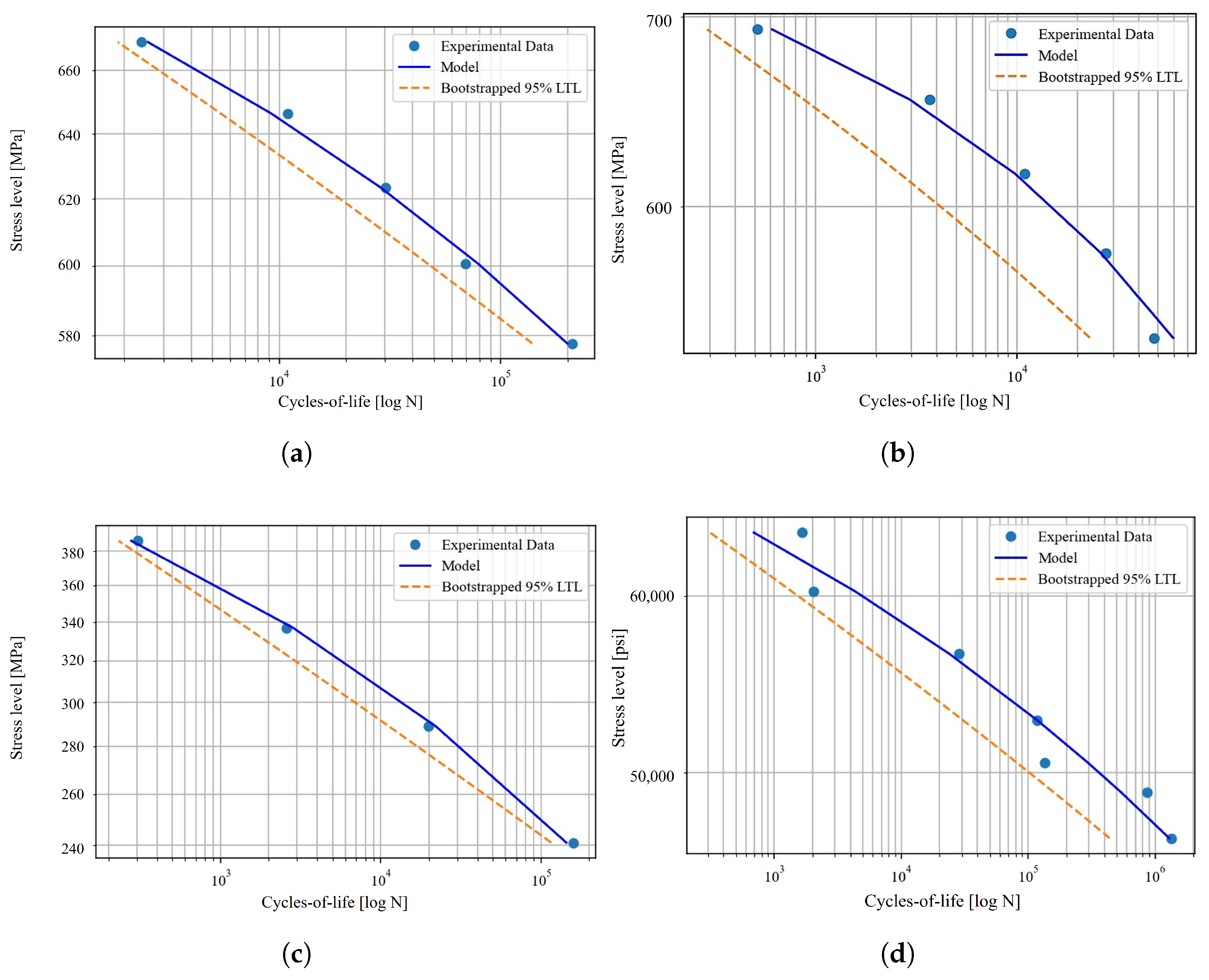
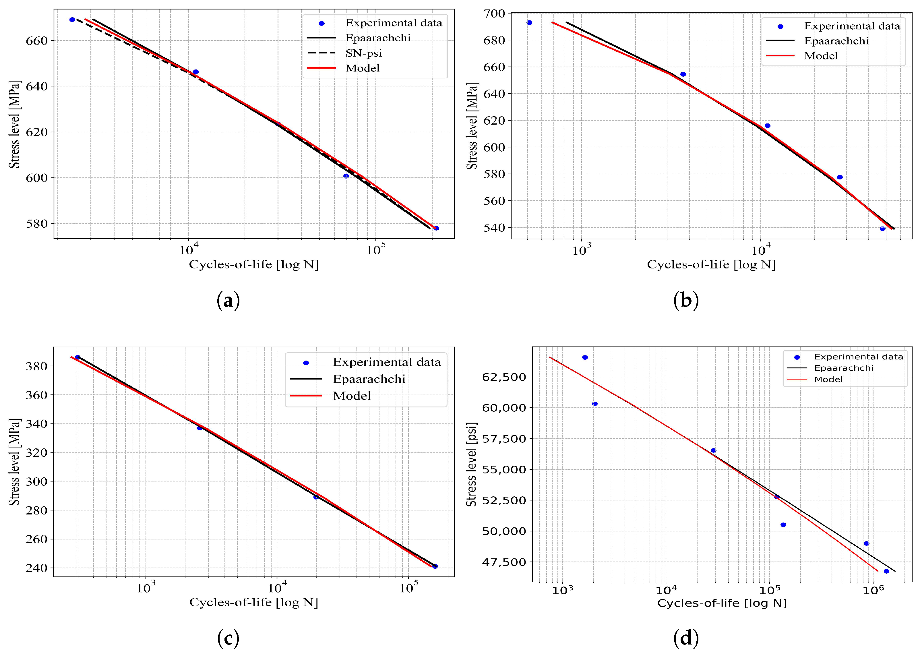
Figure 5a illustrates the model’s performance across various datasets and its comparison with the Eapaarachchi model [36], and in one case with the S–N-φ model developed by An et al. [76]. The material examined by Gao et al. [54], laminated polyether ether ketone ( Gr / P E E K [ 0 / 45 / 9 0 / 45 ] 2 S ), was tested under conditions of R = 0.001 at a frequency of 5 Hz. For this dataset, the proposed model achieved an NMAE value of 0.0178 . Additionally, data from Hwang and Hang [55], along with the corresponding model response, are presented in the Figure 5b. Their experimental work involved E-Glass/epoxy type 1002 composite, tested with R = 0.05 and a frequency of 3 Hertz. The proposed model attained a NMAE value of 0.0408 for this case.
Figure 5c presents data drawn from Broutman and Sahu [56] alongside the corresponding results produced by model application. The experimental investigation utilized E-Glass/epoxy composites with a stress ratio of R = 0.05 and a test frequency of 10 Hz. Model predictions yielded an NMAE value of 0.017 . Yang and Liu [57] (Figure 5d) reported findings from tests on graphite/epoxy laminates under a stress ratio of R = 0.1 and a frequency of 20 Hz. For this dataset, the model achieved an NMAE value of 0.056 .
A comparison with Epaarachchi’s model demonstrates that the difference between the NMAE values of both models is less than 0.04, confirming that these NMAE values are acceptable for predictive purposes.

4.2. Benchmarking Results

Benchmarking involved comparing the predicted fatigue life values with those reported in the literature, utilizing NMAE as a metric to quantify relative performance, identify areas of weakness, and provide justification for acceptance or further development. The model was applied to four different datasets, and its performance regarding the usage of different datasets was validated. The datasets represent stress levels and the number of cycles until failure for different materials, frequencies, and stress ratios. For the calculation of the number of cycles, a normalized expression with compatible units was considered for each one of the datasets here displayed. The experimental results obtained from the benchmarking of various materials were analyzed to conduct a comprehensive fatigue assessment. Table 2 presents the predicted fatigue life for PEEK, while Table 3 and Table 4 provide a summary of the experimental data for E-Glass/Epoxy composites. Additionally, Table 5 compiles the fatigue life data for Graphite/Epoxy under constant amplitude loading conditions.

4.3. LOOCV Results

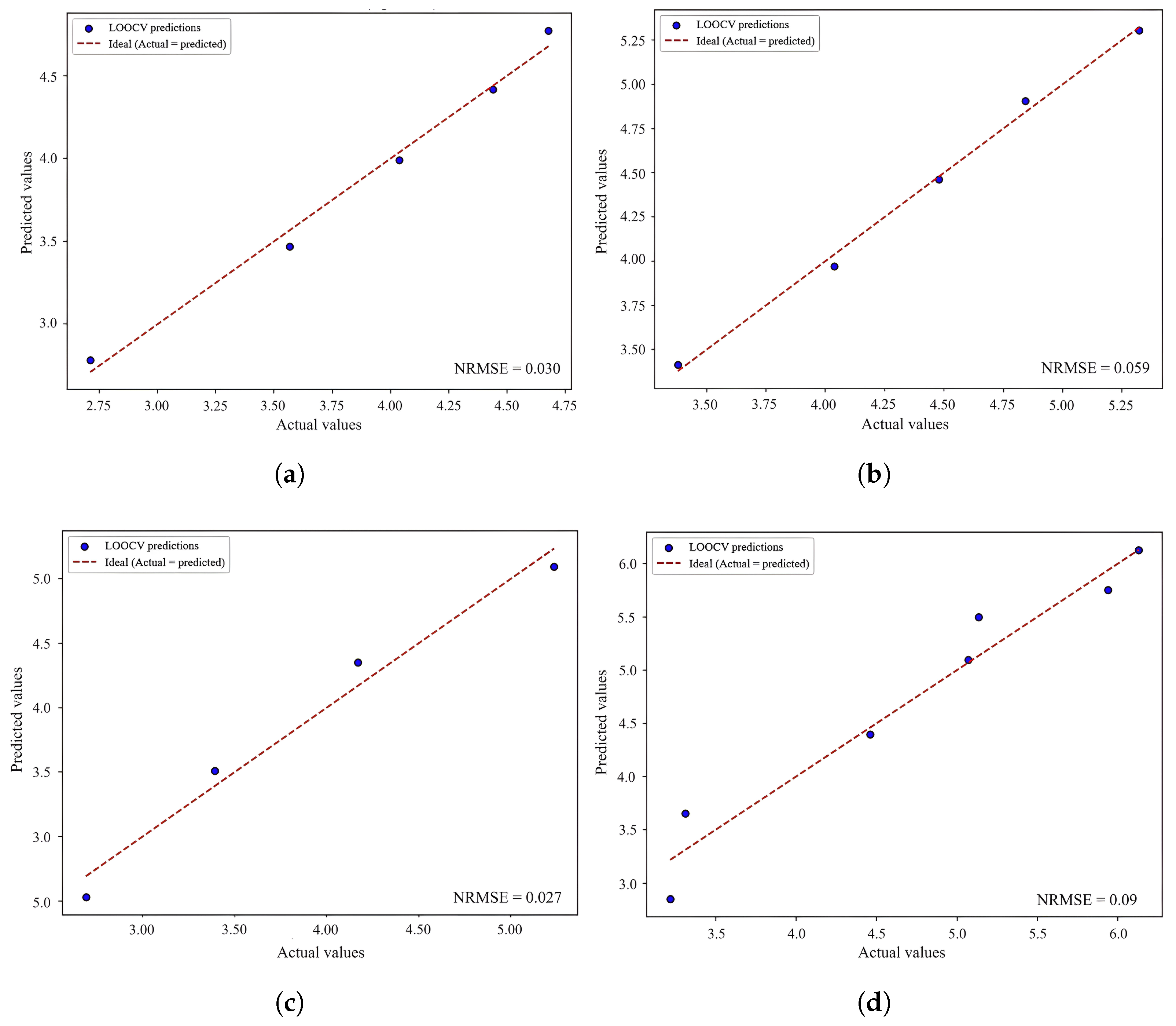
Considering LOOCV procedures, the predictions made from experimental data by applying the model fed the algorithm. The normalized root mean square serves as the parameter that allows the interpretation of the results. LOOCV reaches its own predictions, displayed in Figure 6. NRMSE is shown in each plot.
NRMSE was determined by comparing experimental and predicted values of N. The typical point-wise deviation constitutes only a small percentage of the signal, indicating that any trends or systematic biases are minimal relative to the overall variation in the data. This suggests strong fidelity between the two datasets.

4.4. Identifiability Diagnostics

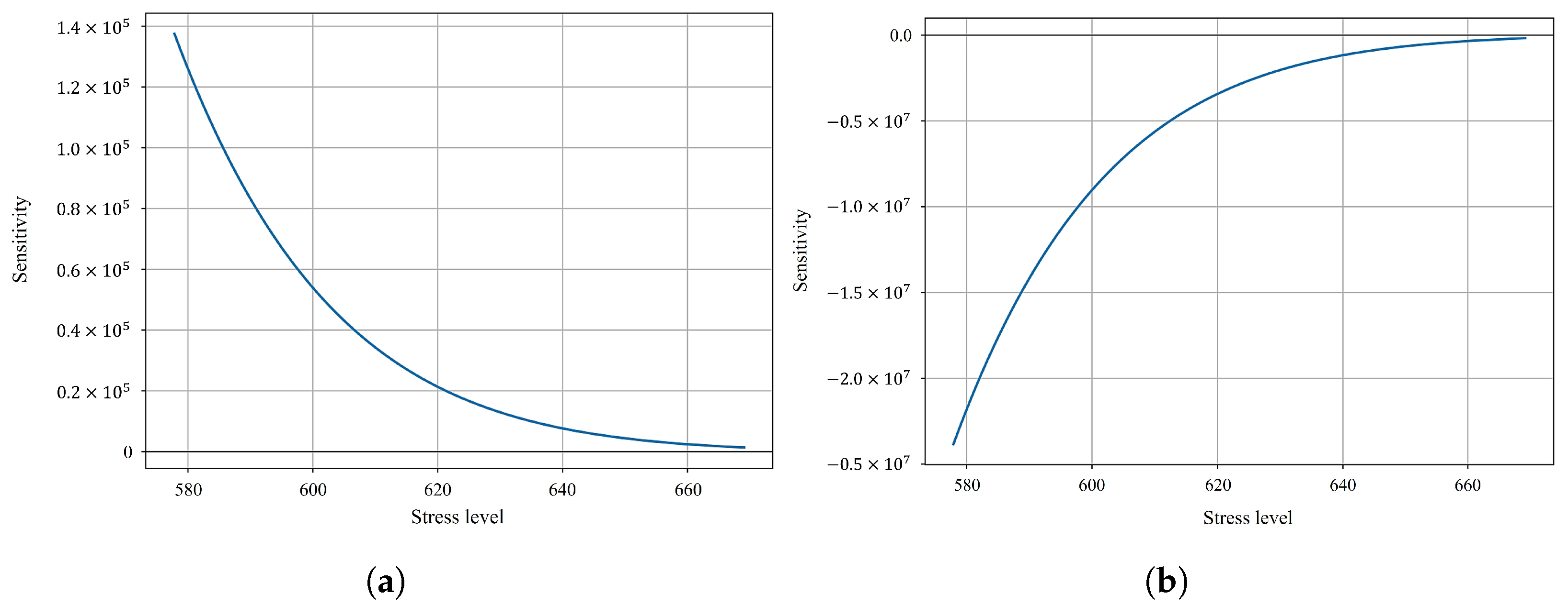
Identifiability analysis is treated here as a necessary condition for fatigue-model credibility. Sensitivity analysis revealed that parameters δ and β influence the response in distinct, non-collinear ways, with δ dominating at low stress and β at high stress (Figure 7). These results show that both parameters are structurally identifiable, but their practical identifiability is strongly dependent on the coverage of the experimental design. Adequate variation across the full stress range is therefore required to constrain δ and β simultaneously.
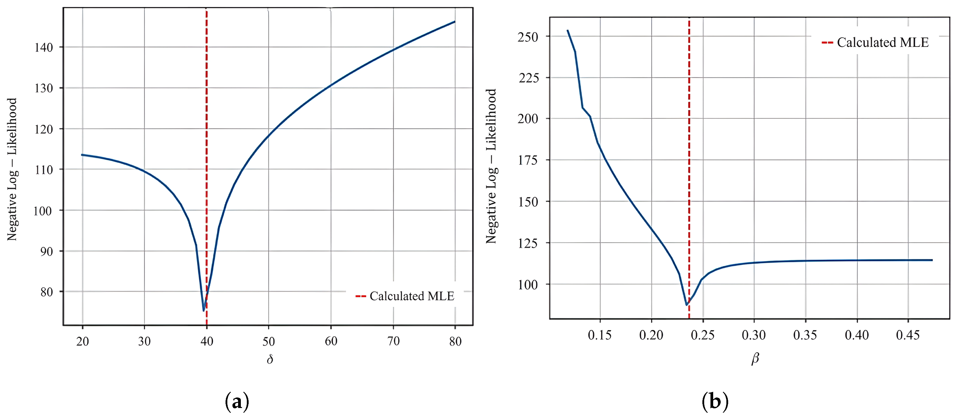
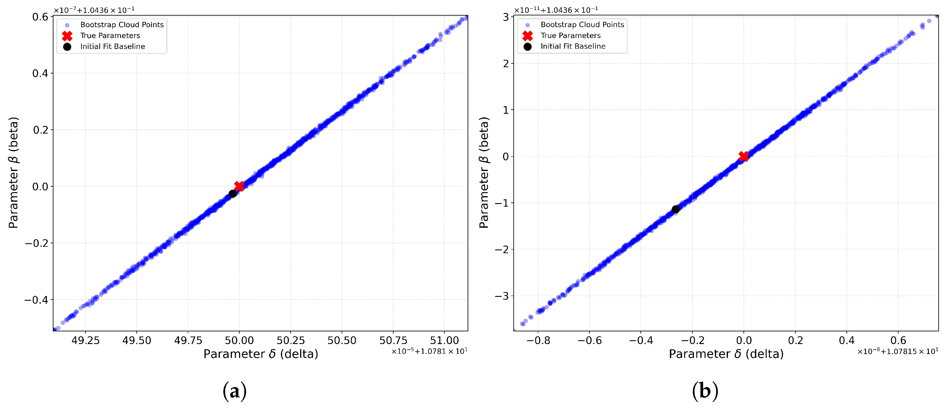
The behavior of the calibrated parameters δ and β across datasets reflects the structure of the proposed residual strength formulation and the characteristics of the experimental matrices used for calibration. Sensitivity analyses show that δ primarily governs the vertical scaling of the S–N response, while β controls the curvature of the fatigue life trajectory. These influences are non-collinear, confirming that the parameters encode distinct aspects of the degradation process rather than redundant effects. This structural separation is further supported by the bootstrap distributions, which form compact, well oriented clusters when the experimental data span a sufficiently broad range of stresses and fatigue lives. Under such conditions, parameter estimates remain stable and practically identifiable. However, if the stress range is narrow or the number of available fatigue levels is limited, the bootstrap clouds elongate along a ridge in parameter space, and profile likelihoods flatten around their minima. This behavior indicates a practical, not structural, identifiability issue. Not a single ( δ , β ) pair can reproduce the available data with similar accuracy. This parameter trade off does not degrade predictive performance within the calibrated domain, because all points along the ridge yield nearly identical S–N curves. Instead, it highlights the dependence of parameter uniqueness on experimental design. Broader stress coverage, additional fatigue levels, or complementary measurements, such as stiffness degradation, would reduce parameter correlation and improve identifiability.
Profile likelihood plots (Figure 8 and Figure 9) show defined minimums for parameters δ and β . Plots exhibit nonlinear effects, and possible parameter trade-offs. These characteristics are inherent to exponential or power forms of models.
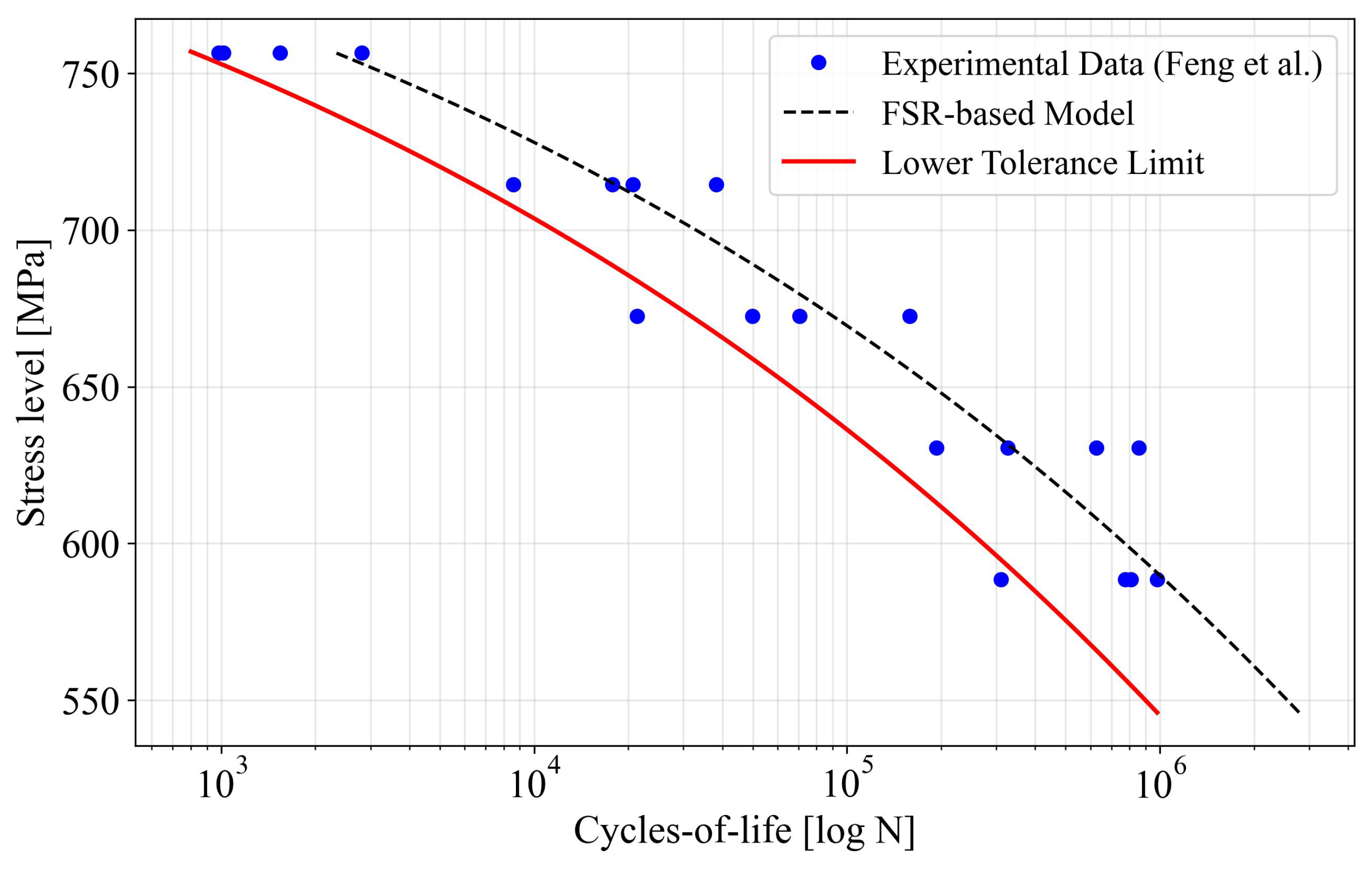
The lower limit tolerance (Figure 10) exhibits a clear boundary for the distribution of N values generated through the model that closely aligns with the experimental results, including the scattered values.
Figure 11 shows the application of the model to a dataset containing dispersed values of N reported by Feng et al. [50]; it is evident that establishing a lower limit is effective for defining a design stress criterion.
The correlation between δ and β does not materially affect predictions within the calibrated stress range, where all parameter combinations along the likelihood ridge yield nearly identical S–N curves. However, this correlation has a pronounced impact on extrapolated predictions, particularly at stresses below the calibration range: different ( δ , β ) pairs that are statistically indistinguishable in range produce increasingly divergent fatigue lives out of range. As a result, uncertainty bands widen substantially at low stresses, and any endurance type extrapolation should be interpreted with caution and accompanied by explicit uncertainty quantification based on the joint ( δ , β ) distribution.

5. Discussion

5.1. Interpretation of Parameter Correlation

The parameter ( f σ ) R is theoretically justified in a prediction life model accounting for the fact that frequency (f) dictates the rate of hysteretic heat generation per unit time, whereas the applied stress ( σ ) defines the magnitude of the thermodynamic driving force for damage evolution. By normalizing the frequency against the load level, the model effectively captures the competition between the molecular mobility of the polymer chains and the intensity of the stress field, providing a proxy for the rate of entropy production and local thermal softening. Consequently, the f S quotient serves to decouple purely mechanical fatigue from accelerated degradation driven by viscous effects. The structure of the index reflects that frequency appears in the numerator to represent the rate of cyclic activation, while stress appears in the denominator and is modulated by the stress ratio R to represent the suppression of viscoelastic relaxation and the onset of creep like dissipation. These two pathways are not interchangeable, and the index does not treat them as such. Higher frequency increases the number of load-unload events per unit time, amplifying cycle dominated damage, whereas higher mean stress increases sustained viscoelastic strain and reduces relaxation time, shifting the response toward creep dominated degradation. This separation is fully consistent with established viscoelastic fatigue mechanics and is precisely why the index can reproduce the observed transition between cycle-controlled a dissipation-controlled regimes in the analyzed datasets. The index therefore does more than correlate with both variables; it assigns them distinct mechanistic roles that reflect the dual nature of damage accumulation in polymer-matrix composites.
The interpretation that higher stress ratios promote more creep-dominated behavior, while lower stress ratios promote more cycle-dominated behavior, is justified for the specific laminated-composite systems and loading regimes represented in the datasets employed. All four datasets correspond to matrix dominated, tension-tension fatigue in polymer matrix composites tested at frequencies where viscoelastic lag, time-dependent strain accumulation, and sustained mean stress effects are known to govern damage evolution. Under these conditions, increasing R elevates the mean stress and reduces the available relaxation time within each cycle, thereby shifting the material response toward creep-like viscoelastic deformation, a trend well documented in classical creep fatigue interaction studies for polymer composites. Lower R values reduce the sustained load component and increase the proportion of reversible cyclic deformation, making the response more cycle-dominated. It is emphasized that this interpretation is not claimed as a universal rule for all composite structures; it applies specifically to the matrix-controlled viscoelastic regimes present in the materials and loading conditions analyzed. Within this scope, however, the R dependent interpretation is both physically consistent and directly supported by the experimental behavior of the systems under study.
The predictive performance trends observed across datasets align with the identifiability characteristics revealed by sensitivity analysis, bootstrap resampling, and profile likelihood diagnostics. Sensitivity curves highlight the distinct and non-collinear influences of the two calibrated parameters: one governs the scaling of the effective damage term, while the other controls the nonlinear accumulation of fatigue life. This structural separation is further supported by bootstrap distributions, which form compact and well-oriented clouds when experimental data cover a wide range of stress levels, loading frequencies, and fatigue lives, indicating stable parameter estimation and minimal practical correlation. Profile likelihoods reinforce these findings, showing well-defined minima for both parameters in datasets with broad coverage of the effective driving term, confirming practical identifiability. Conversely, datasets with narrower loading ranges exhibit greater dispersion in bootstrap samples and flatter profile likelihoods, which explain localized reductions in predictive accuracy. These observations highlight that the model formulation remains robust, with performance variations primarily driven by limitations in the experimental data coverage rather than inherent flaws in the model itself.

5.2. Model Applicability and Limits

The model demonstrates reliability and applicability within the range of stresses, frequencies, and stress ratios represented in the calibration datasets. Within these conditions, the likelihood ridge in the parameter space corresponds to combinations of δ and β that yield similar fatigue-life predictions, ensuring stable interpolation even in the presence of strong parameter correlations. Consequently, the model provides robust fatigue-life estimates for loading scenarios within the experimental domain, with predictions remaining consistent regardless of the specific point chosen along the ridge.
However, limitations arise when the model is applied outside the range of available data. The narrow and elongated ridge observed in bootstrap distributions suggests that different parameter combinations fitting the calibration data equally may diverge under extrapolation, increasing prediction uncertainty under conditions such as lower stresses, untested frequencies, or stress ratios outside the experimental domain. Additionally, the asymmetric curvature of the profile likelihood indicates that one parameter is less strongly informed by the data, amplifying uncertainty when predictions depend heavily on that parameter. Therefore, the model should be used cautiously for extrapolation beyond the tested domain, and any predictions in such regimes should be accompanied by robust uncertainty quantification.

5.3. Comparison with Existing Models

Table 6 shows a comparison between the developed FSR model versus major fatigue-life models cited.

5.4. Practical Implications

The model demonstrates robustness for interpolation within the range of stresses, frequencies, and stress ratios represented in the calibration datasets. Along the likelihood ridge, predicted fatigue lives show minimal variation, ensuring reliable performance for conditions similar to those used during calibration.
However, limitations become evident when the model is applied outside this domain. Under extrapolation, different points along the ridge may diverge, leading to increased uncertainty in predictions for lower stresses, untested frequencies, or stress ratios beyond the experimental range. This highlights the need for explicit uncertainty quantification when using the model in extrapolative scenarios. Methods such as bootstrap-based confidence intervals or likelihood-based bounds are recommended to ensure the reliability of predictions in these regimes.
The findings highlight that the model is robust and reliable for design and assessment tasks within the tested domain, where predictions remain stable despite parameter correlations. However, individual parameters should not be interpreted in isolation, as their estimates represent compensatory trade-offs rather than distinct physical mechanisms. The identifiability analysis reveals opportunities to enhance experimental design by focusing on sensitive regions to reduce uncertainty and parameter correlation. Additionally, the model’s stability makes it suitable for early-stage material evaluations with sparse datasets and supports comparative assessments across materials or processing conditions, provided uncertainty bounds are included for extrapolative predictions. Overall, the evidence confirms the model’s practical applicability and reliability within the experimental domain while emphasizing caution and uncertainty quantification when extending its use beyond the calibration range.

6. Conclusions

The effects of applied stress, stress ratio, and frequency in fatigue testing were considered, and a parameter ( f / σ ) R was introduced to represent the combined influence of these factors on the material’s fatigue behavior under cyclic loading conditions. A fatigue life prediction model for polymer composites was developed. The model generates an S–N curve using parameters such as frequency, stress ratio, static strength, and cycles to failure. An equation with two parameters, informed by experimental data from limited cyclic loading tests, was proposed. The model operates under the assumption that residual strength declines with increasing load cycles n. In the deduction of the model, a specific statistical distribution of data was not considered, nor were negative values of the stress ratio.
The datasets used for model testing incorporate varying frequency and stress ratio values, demonstrating that the model is applicable under different test conditions. It was observed also that the model has a closer approximation to the experimental mean than to the linear approximation. This behavior is observed for only accounting for 4 or 5 scatter values inclusive.
Validation involved comparison with experimental data obtained from different sources and two standard models documented in the literature. The metric employed was the NMAE. The difference between model NMAE and other models NMAE was less than 0.04 in all the observed data.
The robustness of the model was assessed using leave-one-out cross-validation (LOOCV) on predicted cycles to failure, demonstrating good alignment with existing experimental data. NRMSE was the metric used for value comparisons, showing in all the reported cases values less than 0.05 .
After verification that both experimental and predicted data exhibited a strong fit to the Weibull distribution, and based on this, lower limit tolerances for predicted values were proposed, potentially enabling characterization of materials with fewer specimens and at low stress levels, such as during preliminary evaluations prior to comprehensive fatigue life scatter assessment at each stress level.
It was evident that bootstrapping offers possibilities to manage situations where mean ( μ ) and standard deviation ( σ ) are not known and must be estimated from a sample.
Considering that the results of the application of the model were not specific for a determined material, research on the validity of using the term ( f σ ) R as an index of influence to predict fatigue life could be conducted by relating it to the viscoelastic behavior characteristic of polymer composites.

Author Contributions

Conceptualization, M.J.-M.; methodology, J.L.V.-S.; validation, J.L.V.-S. and M.J.-M.; formal analysis, J.L.V.-S. and M.J.-M.; investigation, J.L.V.-S. and M.J.-M.; resources, M.J.-M.; data curation, J.L.V.-S., J.G.R.-R. and A.F.; writing—original draft preparation, J.L.V.-S.; writing—review and editing, J.L.V.-S., C.A.R.-G., U.F.-L., J.G.R.-R. and M.J.-M.; visualization, J.L.V.-S. and M.J.-M.; supervision, M.J.-M. All authors have read and agreed to the published version of the manuscript.

Funding

This research is partially funded by the Kautex Lightweight Structures Lab at Tecnologico de Monterrey Campus Puebla, with the sponsorship of Kautex Textron GmbH.

Data Availability Statement

The original contributions presented in this study are included in the article. Further inquiries can be directed to the corresponding author.

Acknowledgments

The authors are grateful for the support of the students of the lightweight structures lab of Tecnologico de Monterrey, and to the department of Mechanics and Advanced Materials for all the support provided for the development of the applied research projects. The authors appreciate the support of Tecnologico de Monterrey for the Article Processing Charge.

Conflicts of Interest

Author Alvaro Frutos was employed by the company “Kautex Textron de Mexico, S. de R.L. de C.V.”. The remaining authors declare that the research was conducted in the absence of any commercial or financial relationships that could be construed as a potential conflict of interest.

References

  1. Han, H.; Xia, Y.; Ha, S.K. Characterization of Fatigue Properties of Fiber-Reinforced Polymer Composites Based on a Multiscale Approach. Polymers 2025, 17, 157. [Google Scholar] [CrossRef] [Scilit] [PubMed]
  2. Malashin, I.; Masich, I.; Tynchenko, V.; Gantimurov, A.; Nelyub, V.; Borodulin, A.; Martysyuk, D.; Galinovsky, A. Machine Learning in 3D and 4D Printing of Polymer Composites: A Review. Polymers 2024, 16, 3125. [Google Scholar] [CrossRef] [Scilit]
  3. Janssen, R.P.M.; de Kanter, D.; Govaert, L.E.; Meijer, H.E.H. Fatigue Life Predictions for Glassy Polymers: A Constitutive Approach. Macromolecules 2008, 41, 2520–2530. [Google Scholar] [CrossRef] [Scilit]
  4. Yoshimori, S.; Koyanagi, J.; Matsuzaki, R. Efficient Prediction of Fatigue Damage Analysis of Carbon Fiber Composites Using Multi-Timescale Analysis and Machine Learning. Polymers 2024, 16, 3448. [Google Scholar] [CrossRef] [Scilit]
  5. Benabderazag, K.; Guebailia, M.; Belouadah, Z.; Toubal, L.; Tachi, S.E. Machine Learning for Identifying Damage and Predicting Properties in 3D-Printed PLA/Lygeum Spartum Biocomposites. Fibers 2025, 13, 38. [Google Scholar] [CrossRef] [Scilit]
  6. Rooney, K.; Dong, Y.; Basak, A.K.; Pramanik, A. Prediction of Mechanical Properties of 3D Printed Particle-Reinforced Resin Composites. J. Compos. Sci. 2024, 8, 416. [Google Scholar] [CrossRef] [Scilit]
  7. Starkova, O.; Gagani, A.I.; Karl, C.W.; Rocha, I.B.C.M.; Burlakovs, J.; Krauklis, A.E. Modelling of Environmental Ageing of Polymers and Polymer Composites—Durability Prediction Methods. Polymers 2022, 14, 907. [Google Scholar] [CrossRef] [Scilit]
  8. Elkin, A.; Gaibel, V.; Dzhurinskiy, D.; Sergeichev, I. A Multiaxial Fatigue Damage Model Based on Constant Life Diagrams for Polymer Fiber-Reinforced Laminates. Polymers 2022, 14, 4985. [Google Scholar] [CrossRef] [Scilit]
  9. Cheng, Z.Q.; Tan, W.; Xiong, J.J. Progressive damage modelling and fatigue life prediction of Plain-weave composite laminates with Low-velocity impact damage. Compos. Struct. 2021, 273, 114262. [Google Scholar] [CrossRef] [Scilit]
  10. Barriere, T.; Carbillet, S.; Gabrion, X.; Holopainen, S. Prediction of Short- to Long-Term Cyclic Deformation Behavior and Fatigue Life of Polymers. Polymers 2024, 16, 1640. [Google Scholar] [CrossRef] [Scilit] [PubMed]
  11. Zaghloul, M.Y.; Zaghloul, M.M.Y.; Zaghloul, M.M.Y. Influence of Stress Level and Fibre Volume Fraction on Fatigue Performance of Glass Fibre-Reinforced Polyester Composites. Polymers 2022, 14, 2662. [Google Scholar] [CrossRef] [Scilit]
  12. Gonabadi, H.; Oila, A.; Yadav, A.; Bull, S. Fatigue life prediction of composite tidal turbine blades. Ocean Eng. 2022, 260, 111903. [Google Scholar] [CrossRef] [Scilit]
  13. Yang, B.; Aregawi, W.; Chen, R.; Zhang, L.; Wang, Y.; Fok, A.S.L. Accelerated Fatigue Model for Predicting Composite Restoration Failure. J. Dent. Res. 2022, 101, 1606–1612. [Google Scholar] [CrossRef] [Scilit]
  14. Kim, H.S. Theory and Practical Procedure for Predicting S-N Curves at Various Stress Ratios. J. Compos. Biodegrad. Polym. 2019, 7, 57–72. [Google Scholar] [CrossRef] [Scilit]
  15. Movahedi-Rad, A.V.; Eslami, G.; Keller, T. A novel fatigue life prediction methodology based on energy dissipation in viscoelastic materials. Int. J. Fatigue 2021, 152, 106457. [Google Scholar] [CrossRef] [Scilit]
  16. Ma, H.; Bai, X.; Ran, Y.; Wei, X.; An, Z. Modeling the Effect of Stress Ratio, Loading Frequency and Fiber Orientation on the Fatigue Response of Composite Materials. Polymers 2022, 14, 2772. [Google Scholar] [CrossRef] [Scilit]
  17. Kumar, R.; Zafar, S.; Pathak, H.; Subramani, M.; Li, C.; Huang, S.J. Effect of Stress Ratio and Loading Inclination on the Fatigue Life of Carbon-Fiber-Reinforced Polymer Composites: Multiscale Analysis Approach. J. Compos. Sci. 2023, 7, 406. [Google Scholar] [CrossRef] [Scilit]
  18. Amjadi, M.; Fatemi, A. A Fatigue Damage Model for Life Prediction of Injection-Molded Short Glass Fiber-Reinforced Thermoplastic Composites. Polymers 2021, 13, 2250. [Google Scholar] [CrossRef] [Scilit] [PubMed]
  19. Ma, L.; Liu, F.; Liu, D.; Liu, Y. Review of Strain Rate Effects of Fiber-Reinforced Polymer Composites. Polymers 2021, 13, 2839. [Google Scholar] [CrossRef] [Scilit]
  20. Khieng, T.K.; Debnath, S.; Ting Chaw Liang, E.; Anwar, M.; Pramanik, A.; Basak, A.K. A Review on Mechanical Properties of Natural Fibre Reinforced Polymer Composites under Various Strain Rates. J. Compos. Sci. 2021, 5, 130. [Google Scholar] [CrossRef] [Scilit]
  21. Okoli, O.I. The effects of strain rate and failure modes on the failure energy of fibre reinforced composites. Compos. Struct. 2001, 54, 299–303. [Google Scholar] [CrossRef] [Scilit]
  22. Lamnii, H.; Nait Abdelaziz, M.; Ayoub, G.; Colin, X.; Maschke, U. Experimental investigation and modeling attempt on the effects of ultraviolet aging on the fatigue behavior of an LDPE semi-crystalline polymer. Int. J. Fatigue 2021, 142, 105952. [Google Scholar] [CrossRef] [Scilit]
  23. Hirschberg, V.; Wilhelm, M.; Rodrigue, D. Combining mechanical and thermal surface fourier transform analysis to follow the dynamic fatigue behavior of polymers. Polym. Test. 2021, 96, 107070. [Google Scholar] [CrossRef] [Scilit]
  24. Alexis, F.; Castagnet, S.; Nadot-Martin, C.; Robert, G.; Havet, P. Effect of severe thermo-oxidative aging on the mechanical behavior and fatigue durability of short glass fiber reinforced PA6/6.6. Int. J. Fatigue 2023, 166, 107280. [Google Scholar] [CrossRef] [Scilit]
  25. Bogdanov, A.A.; Panin, S.V.; Kosmachev, P.V. Fatigue Damage Assessment and Lifetime Prediction of Short Fiber Reinforced Polymer Composites—A Review. J. Compos. Sci. 2023, 7, 484. [Google Scholar] [CrossRef] [Scilit]
  26. Movahedi-Rad, A.V.; Liu, L.; Keller, T. A novel fatigue life prediction methodology based on energy dissipation in viscoelastic materials, synergistic effects of stress level, stress ratio, and temperature. Int. J. Fatigue 2024, 184, 108296. [Google Scholar] [CrossRef] [Scilit]
  27. Wang, Y.; Wang, Z.; Lv, Y.; Liu, Y. Strength Analysis of Carbon Fiber Composite Flywheel Energy Storage Rotor Based on Progressive Damage Failure. Shock Vib. 2024, 2024, 5587542. [Google Scholar] [CrossRef] [Scilit]
  28. Sakhnevych, A.; Maglione, R.; Timpone, F. A Non-Destructive Methodology for the Viscoelastic Characterization of Polymers: Toward the Identification of the Time–Temperature Superposition Shift Law. Sensors 2023, 23, 9213. [Google Scholar] [CrossRef] [Scilit] [PubMed]
  29. Nosrati, N.; Zabett, A.; Sahebian, S. Stress Dependency of Creep Response for Glass/Epoxy Composite at Nonlinear and Linear Viscoelastic Behavior. Int. J. Polym. Sci. 2022, 2022, 9733138. [Google Scholar] [CrossRef] [Scilit]
  30. Kovačević, D.; Hofman, P.; Rocha, I.; van der Meer, F. Unifying creep and fatigue modeling of composites: A time-homogenized micromechanical framework with viscoplasticity and cohesive damage. J. Mech. Phys. Solids 2024, 193, 105904. [Google Scholar] [CrossRef] [Scilit]
  31. Jayaraman, R. 10–Time-dependent damage evolution in unidirectional and multidirectional polymer composite laminates. In Creep and Fatigue in Polymer Matrix Composites, 2nd ed.; Guedes, R.M., Ed.; Woodhead Publishing Series in Composites Science and Engineering; Woodhead Publishing: Cambridge, UK, 2019; pp. 303–321. [Google Scholar] [CrossRef] [Scilit]
  32. Erartsın, O.; van Drongelen, M.; Govaert, L.E. Identification of plasticity-controlled creep and fatigue failure mechanisms in transversely loaded unidirectional thermoplastic composites. J. Compos. Mater. 2021, 55, 1947–1965. [Google Scholar] [CrossRef] [Scilit]
  33. Zhong, Z.; Wang, F.; Kong, F.; Chen, Y. Study of fatigue damage behavior in off-axis CFRP composites using digital image correlation technology. Heliyon 2024, 10, e25577. [Google Scholar] [CrossRef] [Scilit]
  34. Burhan, I.; Kim, H.S. S-N Curve Models for Composite Materials Characterisation: An Evaluative Review. J. Compos. Sci. 2018, 2, 38. [Google Scholar] [CrossRef] [Scilit]
  35. D’Amore, A.; Grassia, L. Phenomenological approach to the study of hierarchical damage mechanisms in composite materials subjected to fatigue loadings. Compos. Struct. 2017, 175, 1–6. [Google Scholar] [CrossRef] [Scilit]
  36. Epaarachchi, J.A.; Clausen, P.D. An empirical model for fatigue behavior prediction of glass fibre-reinforced plastic composites for various stress ratios and test frequencies. Compos. Part A Appl. Sci. Manuf. 2003, 34, 313–326. [Google Scholar] [CrossRef] [Scilit]
  37. Poursartip, A.; Ashby, M.F.; Beaumont, P.W.R. The fatigue damage mechanics of a carbon fibre composite laminate: I—Development of the model. Compos. Sci. Technol. 1986, 25, 193–218. [Google Scholar] [CrossRef] [Scilit]
  38. Abdo, D.; Gleadall, A.; Silberschmidt, V.V. Damage and damping of short-glass-fibre-reinforced PBT composites under dynamic conditions: Effect of matrix behaviour. Compos. Struct. 2019, 226, 111286. [Google Scholar] [CrossRef] [Scilit]
  39. Katunin, A.; Hufenbach, W.; Kostka, P.; Holeczek, K. Frequency dependence of the self-heating effect in polymer-based composites. J. Achiev. Mater. Manuf. Eng. 2010, 41, 9–15. [Google Scholar]
  40. LY, M.; Khan, K.; Muliana, A. Analyzing the Effect of Energy Dissipation on Thermo-Mechanical Responses of Viscoelastic Fiber Reinforced Composites Using Finite Element Method. In American Society for Composites 2017; DEStech Publications, Inc.: Lancaster, PA, USA, 2017. [Google Scholar] [CrossRef] [Scilit]
  41. Katunin, A.; Krukiewicz, K. Physicochemical analysis of self-heating of glass-epoxy composites cured by novolac. CHEMIK Nauka-Tech.-Rynek 2012, 66, 1326–1331. [Google Scholar]
  42. Sahputra, I.; Echtermeyer, A. Creep–Fatigue Relationship in Polymer: Molecular Dynamics Simulations Approach. Macromol. Theory Simul. 2014, 24, 65–73. [Google Scholar] [CrossRef] [Scilit]
  43. Oguma, H.; Naito, K. Effects of mean stress on the fatigue properties of core-in-sheath-type carbon/glass hybrid thermoplastic composite rods: Experimental investigation and practical predictive method. Fatigue Fract. Eng. Mater. Struct. 2024, 47, 2922–2933. [Google Scholar] [CrossRef] [Scilit]
  44. Degrieck, J.; Van Paepegem, W. Fatigue damage modeling of fibre-reinforced composite materials: Review. Appl. Mech. Rev. 2001, 54, 279–300. [Google Scholar] [CrossRef] [Scilit]
  45. Hwang, W.; Han, K. Fatigue of Composite Materials—Damage Model and Life Prediction. In Composite Materials: Fatigue and Fracture, Second Volume; ASTM International: West Conshohocken, PA, USA, 1989. [Google Scholar] [CrossRef] [Scilit]
  46. Sendeckyj, G.P. Fitting Models to Composite Materials Fatigue Data. In Test Methods and Design Allowables for Fibrous Composites; ASTM International: West Conshohocken, PA, USA, 1981. [Google Scholar] [CrossRef] [Scilit]
  47. D’Amore, A.; Grassia, L. Comparative Study of Phenomenological Residual Strength Models for Composite Materials Subjected to Fatigue: Predictions at Constant Amplitude (CA) Loading. Materials 2019, 12, 3398. [Google Scholar] [CrossRef] [Scilit]
  48. D’Amore, A.; Giorgio, M.; Grassia, L. Modeling the residual strength of carbon fiber reinforced composites subjected to cyclic loading. Int. J. Fatigue 2015, 78, 31–37. [Google Scholar] [CrossRef] [Scilit]
  49. Epaarachchi, J.A.; Clausen, P.D. A new cumulative fatigue damage model for glass fibre reinforced plastic composites under step/discrete loading. Compos. Part A Appl. Sci. Manuf. 2005, 36, 1236–1245. [Google Scholar] [CrossRef] [Scilit]
  50. Feng, Y.; Ma, B.; Zhang, T.; Zhang, T.; He, Y.; Jiao, S. Reliability Fatigue Life and A New S–N Curve Model of Composite Laminates Under Tensile-Tensile Fatigue Load. Appl. Compos. Mater. 2021, 28, 129–148. [Google Scholar] [CrossRef] [Scilit]
  51. Petrini, L.; Bertini, A. A three-dimensional phenomenological model describing cyclic behavior of shape memory alloys. Int. J. Plast. 2020, 125, 348–373. [Google Scholar] [CrossRef] [Scilit]
  52. Fernández-Canteli, A.; Castillo, E.; Blasón, S. A methodology for phenomenological analysis of cumulative damage processes. Application to fatigue and fracture phenomena. Int. J. Fatigue 2021, 150, 106311. [Google Scholar] [CrossRef] [Scilit]
  53. Mozafari, F.; Thamburaja, P.; Srinivasa, A.; Abdullah, S. Fatigue life prediction under variable amplitude loading using a microplasticity-based constitutive model. Int. J. Fatigue 2020, 134, 105477. [Google Scholar] [CrossRef] [Scilit]
  54. Gao, J.; Zhu, P.; Yuan, Y.; Wu, Z.; Xu, R. Strength and stiffness degradation modeling and fatigue life prediction of composite materials based on a unified fatigue damage model. Eng. Fail. Anal. 2022, 137, 106290. [Google Scholar] [CrossRef] [Scilit]
  55. Hwang, W.; Han, K. Cumulative Damage Models and Multi-Stress Fatigue Life Prediction. J. Compos. Mater. 1986, 20, 125–153. [Google Scholar] [CrossRef] [Scilit]
  56. Broutman, L.J.; Sahu, S. A New Theory to Predict Cumulative Fatigue Damage in Fiberglass Reinforced Plastics. In Composite Materials: Testing and Design (Second Conference); ASTM International: West Conshohocken, PA, USA, 1972. [Google Scholar] [CrossRef] [Scilit]
  57. Yang, J.; Liu, M. Residual Strength Degradation Model and Theory of Periodic Proof Tests for Graphite/Epoxy Laminates*. J. Compos. Mater. 1977, 11, 176–203. [Google Scholar] [CrossRef] [Scilit]
  58. Hodson, T.O. Root-mean-square error (RMSE) or mean absolute error (MAE): When to use them or not. Geosci. Model Dev. 2022, 15, 5481–5487. [Google Scholar] [CrossRef] [Scilit]
  59. Wang, W.; Lu, Y. Analysis of the Mean Absolute Error (MAE) and the Root Mean Square Error (RMSE) in Assessing Rounding Model. IOP Conf. Ser. Mater. Sci. Eng. 2018, 324, 012049. [Google Scholar] [CrossRef] [Scilit]
  60. de Lange, A.M.G.; Anatürk, M.; Rokicki, J.; Han, L.K.M.; Franke, K.; Alnæs, D.; Ebmeier, K.P.; Draganski, B.; Kaufmann, T.; Westlye, L.T.; et al. Mind the gap: Performance metric evaluation in brain-age prediction. Hum. Brain Mapp. 2022, 43, 3113–3129. [Google Scholar] [CrossRef] [Scilit]
  61. Roider, J.; Nguyen, A.; Zanca, D.; Eskofier, B.M. Assessing the Performance of Remaining Time Prediction Methods for Business Processes. IEEE Access 2024, 12, 130583–130601. [Google Scholar] [CrossRef] [Scilit]
  62. Gaurav, A. Data-driven machine learning regression methods to predict the residual strength in FRP composites subjected to fatigue. Polym. Compos. 2025, 46, 10713–10733. [Google Scholar] [CrossRef] [Scilit]
  63. Khadka, N. How Leave-One-Out Cross Validation (LOOCV) Improve’s Model Performance. Dataaspirant Data Sci. Portal Begin. 2023, 5, 542–548. [Google Scholar]
  64. Dinh, T.D.; Han, S.; Yaghoubi, V.; Xiang, H.; Erdelyi, H.; Craeghs, T.; Segers, J.; Van Paepegem, W. Modeling detrimental effects of high surface roughness on the fatigue behavior of additively manufactured Ti-6Al-4V alloys. Int. J. Fatigue 2021, 144, 106034. [Google Scholar] [CrossRef] [Scilit]
  65. Xiang, G.; Bacharoudis, K.C.; Vassilopoulos, A.P. Probabilistic fatigue model for composites based on the statistical characteristics of the cycles to failure. Int. J. Fatigue 2022, 163, 107085. [Google Scholar] [CrossRef] [Scilit]
  66. Nickens, D.J. Using Tolerance Limits to Evaluate Laboratory Data. Drug Inf. J. DIJ/Drug Inf. Assoc. 1998, 32, 261–269. [Google Scholar] [CrossRef] [Scilit]
  67. Datta, D.; Mishra, S.; Rajest, S.S. Quantification of tolerance limits of engineering system using uncertainty modeling for sustainable energy. Int. J. Intell. Netw. 2020, 1, 1–8. [Google Scholar] [CrossRef] [Scilit]
  68. Catalanotti, G. Uncertainty quantification for advanced progressive damage models for composites by means of efficient emulators and bootstrapping. Compos. Part A Appl. Sci. Manuf. 2022, 163, 107238. [Google Scholar] [CrossRef] [Scilit]
  69. Abu Bakar, S.; Hussain, S.I.; Mourad, Z. Optimizing Degradable Plastic Density Prediction: A Coarse-to-Fine Deep Neural Network Approach. Sains Malays. 2024, 53, 447–459. [Google Scholar] [CrossRef] [Scilit]
  70. Kloppenborg, S. cmstatr: An R Package for Statistical Analysis of Composite Material Data. J. Open Source Softw. 2020, 5, 2265. [Google Scholar] [CrossRef] [Scilit]
  71. Fong, J.; Cimini, C.; Melo, J.; Heckert, N.; Filliben, J. Theoretical Failure Envelopes of Open Hole Composite Laminates with A- and B-Basis Allowables Estimated from Smooth Specimen Properties. In Proceedings of the 19th International Conference of Composite Materials, Montreal, QC, Canada, 29 July–1 August 2013. [Google Scholar]
  72. Nettles, A.T. Allowables for Structural Composites. In International Conference on Composites Engineering; ICCE: New Orleans, LA, USA, 2004. [Google Scholar]
  73. Gonçalves, S.; Kilian, L. Bootstrapping autoregressions with conditional heteroskedasticity of unknown form. J. Econom. 2004, 123, 89–120. [Google Scholar] [CrossRef] [Scilit]
  74. Meeker, W.Q.; Escobar, L.A. Statistical Methods for Reliability Data; Wiley: Hoboken, NY, USA, 1998. [Google Scholar]
  75. Jiang, S.; Zhang, W. A hybrid approach of modified bootstrap and physics-based methods for probabilistic fatigue life prediction considering overload effects. Probabilistic Eng. Mech. 2022, 70, 103343. [Google Scholar] [CrossRef] [Scilit]
  76. An, H.; Zhao, W. Fatigue life prediction for composite materials based on the S-N-φ model. AIP Adv. 2023, 13, 085328. [Google Scholar] [CrossRef] [Scilit]
Figure 1. Conceptual representation of cycle-dominated and time-dominated fatigue regimes in polymer composites and the frequency–stress–ratio (FSR) index as a phenomenological descriptor of the continuous transition between these regimes.
Designs 10 00063 g001
Figure 2. Sensitivity of damage per cycle to f / σ parameter values, according to function D = σ 0 ( f / σ ) R , employing σ 0 = 760 MPa, 20 σ 80 for three values of f, (a) R = 0.5 , (b) R = 0.1 .
Designs 10 00063 g002
Figure 3. Sensitivity to number of cycles according to function N = ( δ ( 1 σ σ 0 ) ( f / σ ) R ) ( 1 / β ) , employing σ 0 = 760 MPa, in ranges 0 f 20 ; 577 σ 669 for: (a) R = 0.01 , (b) R = 0.1 , (c) R = 0.5 , (d) R = 0.8 .
Designs 10 00063 g003
Figure 4. General guideline to obtain a residual strength degradation model [46,47].
Designs 10 00063 g004
Figure 5. Semi-log S–N curves generated using the proposed model according to different datasets: (a) Proposed model with δ = 10.7815 and β = 0.10436 ( S u = 760 MPa, R = 0.001 , f = 5 Hz [54]). (b) Proposed model with δ = 28.62908 and β = 0.21363 ( S u = 770 MPa and R = 0.05 , f = 3 Hz [55]). (c) Proposed model with δ = 1.57738 and β = 0.0547 ( S u = 483 MPa and R = 0.05 , f = 3 Hz [56]). (d) Proposed model with δ = 2.12318 and β = 0.0547 ( S u = 75,390 psi and R = 0.1 , f = 20 Hz [57]).
Designs 10 00063 g005
Figure 6. Actual number of cycles until failure (model) versus model LOOCV values (Logarithmic scale), (a) Hwang and Hang data [55]. δ = 31.18 and β = 0.2208 , (b) Gao et al. [54] data δ = 10.886 and β = 0.1013 , (c) Broutman and Sahu data [56]. δ = 1.4662 and β = 0.05176 , (d) Yang data [57]. δ = 1.4869 and β = 0.04153 .
Designs 10 00063 g006
Figure 7. Sensitivity of number of cycles until failure (N) to model parameters: (a) parameter δ , (b) parameter β .
Designs 10 00063 g007
Figure 8. Profile likelihood of model parameters, (a) parameter δ , (b) parameter β . Maximum Likelihood Estimation (MLE) was applied to identify the parameter values that maximize data likelihood, with the negative log-likelihood (NLL) minimum marking the optimal estimate and its curvature indicating sensitivity and uncertainty.
Designs 10 00063 g008
Figure 9. Bootstrap cloud of model parameters δ and β , (a) narrow stress range, (b) wide stress range.
Designs 10 00063 g009
Figure 10. S–N curve predicted by the proposed model from various reference datasets showing the lower tolerance limit obtained with bootstrapping: (a) Gao et al. data [54]. δ = 10.7815 and β = 0.10436 , (b) Hwang and Hang data [55]. δ = 28.62908 and β = 0.21363 , (c) Broutman and Sahu data [56]. δ = 1.4662 and β = 0.05176 , (d) Yang data [57]. δ = 1.4869 and β = 0.04153 .
Designs 10 00063 g010
Figure 11. S–N curve predicted by the model; bootstrapping lower limit tolerance for scattered cyclic life of composite material T700/MTM46 reported by Feng et al. [50].
Designs 10 00063 g011
Table 1. Coupling of f, applied stress σ and R in a FSR index.
VariableRole in Dissipation-Controlled FatigueReferences
Frequency fScales power input and self-heating rate[22,23,25]
Applied stress σ Governs mechanical work and creep/plasticity[22,24,25,26]
Stress ratio RTunes cyclic vs. creep contribution and nonlinearity[7,22,25,26]
Indicator FSR basedPhenomenological measure of damage-driving power[7,22,23,24,25,26]
Table 2. NMAE for predicted fatigue life data of G r / P E E K [ 0 / 45 / 90 / 45 ] 2 S tested by Gao et al. [54] laminates under constant amplitude cyclic loading. The proposed model accounts for δ = 10.7815 and β = 0.10436 ; R = 0.001; f = 5 Hz; σ u = 760 MPa.
Stress Level [MPa]Mean Value of Fatigue Life [Cycles]Model Calculated N [Cycles]S–N- φ Calculated N [Cycles]Epaarachchi-Calculated N [Cycles]NMAE ModelNMAE S–N- φ NMAE Epaarachchi
669.122388282925212730
646.3110,91810,05796769283
623.5030,08430,82130,00528,1180.01780.0270.017
600.6869,40484,03680,45078,377
577.87210,156208,280194,206205,299
Table 3. Experimental data from Hwang and Han [55] on E-Glass/epoxy Uni-directional composite type 1002, δ = 28.62908 and β = 0.21363 ( σ u = 770 MPa and R = 0.05, f = 3 Hz).
Stress Level [MPa]Mean Value of Fatigue Life [Cycles]Model Calculated N [Cycles]Epaarachchi-Calculated N [Cycles]NMAE ModelNMAE Epaarachchi
693.0513690463
654.5369431103590
616.010,922976211,8630.0450.048
577.527,57724,60529,949
539.047,73953,52255,699
Table 4. Experimental data published by Broutman and Sahu [56] for E-Glass/epoxy [08/908]. Model uses values of δ = 1.57738 and β = 0.0547 ( σ u = 483 MPa and R = 0.05, f = 10 Hz).
Stress Level [MPa]Mean Value of Fatigue Life [Cycles]Model Calculated N [Cycles]Epaarachchi-Calculated N [Cycles]NMAE ModelNMAE Epaarachchi
386304271301
337258327922623
28919,86121,94219,9670.0240.0004
241158,994145,461158,829
Table 5. Fatigue life data of graphite/epoxy laminates under constant amplitude cyclic [57]. Proposed model with δ = 2.12318 and β = 0.0547 ( σ u = 75,390 psi and R = 0.1; f = 20 Hz).
Stress Level [psi]Mean Value of Fatigue Life [Cycles]Model Calculated N [Cycles]Epaarachchi-Calculated N [Cycles]NMAE ModelNMAE Epaarachchi
64,0821650754808
60,312205075844610
56,54328,73024,23023,679
52,773117,580113,983114,1830.0800.053
50,511135,500275,133288,489
49,003863,200486,380533,282
46,7411,346,3001,115,8121,338,510
Table 6. Characteristics of FSR model vs. major fatigue-life models cited.
FeatureFSR ModelEpaarachchi–ClausenSendeckyj-Equivalent StrengthD’Amore–Grassia Residual StrengthAn–Zhao [76] S–N- φ
Incorporates stress ratio RYes (explicit)YesYesYesYes
Incorporates frequency fYes (explicit)Yes (empirical)LimitedNoNo
Theoretical basisPhenomeno-logicalEmpiricalSemi-mechanisticPhenomeno-logicalProbabilistic
Number of parameters2 ( δ , β )3–52–32–33
Probabilistic outputYes (bootstrap LTL)NoOptionalNoYes
Handling of limited dataYes (LOOCV + bootstrap)ModerateModerateModerateYes
Validated across different materialsYesYesYesYesYes
Captures viscoelastic effectsIndirectly ( f / σ )PartiallyNoNoNo
Applicability to variable amplitudeNot validatedYesLimitedYesLimited
ContributionUnified FSR term + probabilistic LTL + validation procedureStress-ratio/frequency empirical correctionsEquivalent static strength mappingHierarchical damageStatic strength-based S–N mapping
Disclaimer/Publisher’s Note: The statements, opinions and data contained in all publications are solely those of the individual author(s) and contributor(s) and not of MDPI and/or the editor(s). MDPI and/or the editor(s) disclaim responsibility for any injury to people or property resulting from any ideas, methods, instructions or products referred to in the content.