Article

Anisotropic k-ϵ Model Based on General Principles of Statistical Turbulence

by
J. J. H. Brouwers
Romico Hold.VBA, 6226 GV Maastricht, The Netherlands
Inventions 2024, 9(5), 95; https://doi.org/10.3390/inventions9050095
Submission received: 22 July 2024 / Revised: 20 August 2024 / Accepted: 27 August 2024 / Published: 29 August 2024

Abstract

:
An upgrade is presented of a recently published model for the calculation of statistical averages of turbulent flow variables. Instead of empirical constructions, important parts of the model are based on general principles of statistical turbulence and physics. The upgrade concerns transparent and simplified descriptions of turbulent diffusion and Reynolds stresses which express their dependency of mean flow gradients in a direct manner. As before, prediction comparisons are satisfactory in relation to the results of DNS of channel flow. Implementation in a CFD code is straightforward and its application provides a significant improvement to the results of the widely used empirical basic k- ϵ model.

1. Introduction

Models of computational fluid dynamics (CFD) are generally based on semi-empirical descriptions of diffusion by turbulent fluctuations [1,2]. This includes the basic k- ϵ model widely used in engineering and environmental analysis and offered in software packages [3,4]. Recently, a new model was presented [5]. Instead of empiricism, it rested on the application of general principles and properties of statistical turbulence. Predictions of the new model compared favourably with the results of direct numerical simulations (DNS) of channel flow at a large Reynolds number [6,7,8]. This contrasted with the predictions of the basic k- ϵ model which showed remarkable differences.
In the present paper, an upgrade and generalisation of the new model is given. As before, it is tested against DNS of channel flow. Equations are presented in a form which enable straightforward implementation in CFD codes.

2. Averaged Conservation Equations

Equations are presented for the calculation of the average values of fluctuating variables in turbulent flows. The flow is that of a fluid with constant or almost constant density ρ , e.g., a liquid or a gas at subsonic speed. Turbulent fluctuations measured at a fixed point in space are treated as a statistical process which is stationary or almost stationary in time compared to the time of velocity fluctuations. Statistical averages follow from time averaging over sufficiently long time intervals. The time averaged representation of the Navier–Stokes equations is given by
  • Conservation of mass:
u i x i = 0
  • Conservation of momentum:
u i t + u j u i x j + < u i u j > x j = p x i
  • Conservation of energy:
θ t + u j θ x j + < u j θ > x j = 0
where angled brackets represent statistical averaging, t and x are time and space coordinate, u, p, and θ are mean or time-averaged values of fluid velocity, pressure, and temperature, respectively, and u and θ represent fluctuations of velocity and temperature, respectively, that is, the velocity and temperature minus their mean value. Throughout this paper, repeated indices imply summation unless otherwise stated. As we were concerned with flow at a high Reynolds number, the contributions of the viscous forces and heat conductivity present in the Navier–Stokes equations were dropped. Their effect can be disregarded when considering the main flow governed by the instability of inviscid flow outside small boundary layers. The average temperature in energy within Equation (3) can also be used to describe the average distribution of passive or almost passive admixture in the fluid.

3. Diffusion Representations of Turbulent Fluxes

The appearance of turbulent fluxes in the convection terms of the averaged conservation equations results in an unclosed set of equations for mean flow variables. To resolve this issue, descriptions of the turbulent flux terms were derived, which are based on general principles of statistical turbulence at a large Reynolds number [5,9]. The derivation starts from the formulation of a Langevin or fluctuation equation and the associated Fokker Planck or diffusion equation for the velocity and position of a marked fluid particle [10,11,12,13]. The approach is known from molecular dynamics and related stochastic problems [14,15,16,17] yielding the descriptions of the transport coefficients of viscosity, thermal conductivity, and diffusion of dilute gases [17,18]. Challenges in the case of turbulence are the inhomogeneous and anisotropic nature of turbulence, dissipation of energy, and general specification of the coefficients of the equations by Eulerian statistical values of flow.
The following principles and properties were invoked:
-
The formulation of a Langevin equation for fluid particle velocity is in accordance with the property that autocorrelations of particle accelerations are vanishingly short compared to those of velocities in the limit of a large Reynolds number [19].
-
Kolmogorov’s similarity theory holds for the small viscous scales of turbulence [19]; it is an inertial subrange representation that specifies the white noise term in the Langevin equation.
-
Solutions of the Langevin and diffusion equation are presented by a perturbation expansion in powers of the inverse of the Kolmogorov constant C 0 [8,9,10,11]. Matching predictions with data of measurements and DNS reveal values of C 0 around 6–7 [10,11,12,13,20,21]. In the present analysis, C 0 = 7 .
-
The time scale of velocity fluctuations and its decorrelation scales as C 0 1 compared to the time scale of energy dissipation. It enables us to treat the first term of the solution as a Hamiltonian process and to apply the fluctuation–dissipation theorem and Onsager symmetry [14,15,16,17].
-
The well-mixing principle of Lagrangian and Eulerian velocities [22] enables to specify the second term in the expansion of the diffusion result.
-
Particle displacement during velocity correlation scales as C 0 1 compared to the scale of inhomogeneity, enabling the Lagrangian formulation to be converted in an Eulerian one [9,13].
Results for turbulent fluxes of momentum and conservative scalars are as follows [5,9,13]:
  • Momentum flux
< u j u i > = 2 3 k 0 δ i j D i k u j x k D j k u i x k
  • Temperature flux (and flux of any conservative scalar)
< u j θ > = D j k θ x k
In Equation (4), δ i j is Kronecker delta and k 0 is the kinetic energy of the isotropic state. It is the analogue of the kinetic energy of translating gas molecules [23]. The value of k 0 follows from the equation for kinetic energy presented in the next section.
The diffusion coefficient D i j in Equations (4) and (5) is specified by [5,9,13]
D i j = 2 C 0 1 ϵ 1 σ i n σ n j + 2 C 0 2 ϵ 2 σ l i σ j k u n σ l k x n 4 C 0 2 ϵ 1 σ k j u n x n ( ϵ 1 σ i m σ m k )
where
σ i j = < u i u j >
ϵ is the energy dissipation rate whose governing equation is presented in Section 5, and C 0 = 7 is the Kolmogorov constant.
Implementing the above expressions in Equation (4) results in a set of algebraic relations of the covariance tensor σ i j in terms of k 0 and mean velocity gradients. Solving these non-linear coupled equations for given k 0 and mean velocity gradients can pose some problems due to multi-valued dependencies between variables in specific areas of the flow field [5]. An alternative formulation which circumvents such problems is obtained by the following procedure. The diffusion coefficients on the right-hand side of Equation (4) represent a certain state which is altered by the gradients of the mean flow, leading to a new state of covariance values described by the left-hand side of Equation (4). This principle can be applied to any state. It can be applied to a basic isotropic state σ i j = 2 3 k 0 δ i j . The thus-determined new state can serve as the basis for the calculation of the next state. This process can be continued up to and including terms of O ( C 0 2 ) . The result inhibits the same truncation error as the original formulation, cf. Equation (6). For the diffusion coefficient D i k , we obtain
D i k = 8 9 k 0 2 C 0 ϵ δ i k 4 k 0 3 ( 4 3 k 0 C 0 ϵ ) 2 ( u k x i + u i x k ) + 16 k 0 6 27 C 0 2 ϵ 4 ( u n x n ( ϵ 2 k 0 3 ) ) δ i k
while the covariance tensor σ i j is given by Equation (4) with the diffusion coefficients according to Equation (8). For kinetic energy k = σ i i 2 , we can write
k = k 0 ( 1 + 1 3 ( 4 k 0 3 C 0 ϵ ) 2 ( u i x j + u j x i ) 2 )
which relates k to the isotropic value of kinetic energy k 0 . The second term on the RHS of this equation describes the increase in kinetic energy associated with the anisotropy of turbulent fluctuations. The expression is obtained upon implementing the description for σ i i according to Equations (4) and (8) and making use of the equation of continuity Equation (1).
The last term of the RHS of Equation (8) originates from the O ( C 0 2 ) terms in Formulation (6). The term complies with the decaying part of kinetic energy and dissipation of homogeneous isotropic turbulence behind a grid [11,12,13]. The second term on the RHS of Equations (8) and (9) describes contributions, which are associated with the anisotropy caused by main flow gradients.
The presented descriptions are valid up to a truncation error of O ( C 0 3 ) . They are the result of applying general principles and do not involve empiricism nor calibration factors.

4. Equation for Kinetic Energy

A closed set of equations is obtained upon formulating equations for k connected to k 0 through Equation (9), as well as ϵ . For both variables, equations can be derived from the Navier–Stokes equations. For k, we can write [7,8]
k t + u i k x i + < u i k > x i + ρ 1 < u i p > x i = P ϵ
where P is the mean production of energy via turbulent fluctuations defined by
P = σ i j u i x j
and where k and p are the fluctuating parts of kinetic energy and pressure, respectively, that is, the kinetic energy and dissipation rates minus their time-averaged values. There are two turbulent flux terms in Equation (10), i.e., the third and fourth term on the LHS of Equation (10), which need to be modelled. Equation (5) is valid for a conservative scalar, while kinetic energy and pressure are non-conservative variables. An approximate approach is to treat the sum of the two flux terms as a conservative scalar proceeded by a calibration constant c k , which corrects for non-conservative behaviour [5].
< u i k > + ρ 1 < u i p > = c k D i j k x j
Comparison with DNS of channel flow reveals c k = 1.3 ; the dependency on distance from the channel wall is found to be well described by D i j [5].
Substituting for σ i j in Equation (11), as well as using Equations (4), (7) and (8) and making use of the equation of continuity Equation (1) yields the following:
P = ( 9 C 0 T 2 8 k 0 2 ) ϵ
where T 2 is determined by shear stresses:
T 2 = σ 12 2 + σ 23 2 + σ 13 2
which are specified by Equations (4) and (8). Thus, the following equation for kinetic energy is obtained:
k t + u i k x i = c k x i ( D i j k x j ) + ( 9 C 0 T 2 8 k 0 2 1 ) ϵ
where k can be replaced by k 0 using Equation (9), resulting in an equation specifying k 0 . The equation describes the change of k 0 due to energy production and dissipation (the last term on RHS), diffusion of energy (the first term on the RHS), and energy convection (the term on the LHS). In case of the random motion of gasmolecules, k 0 is a constant depending on temperature. In case of turbulence, k 0 changes in value according to Equation (15).

5. Equation for Energy Dissipation

The basic form of the equation for energy dissipation obtained from the Navier–Stokes equations contains a number of terms which are governed by the small viscous scales of turbulence [1,2]. The terms can be replaced by expressions that meet the criteria of matching the results of decaying grid turbulence and the log layer of wall-induced turbulence [1,2].
ϵ t + u i ϵ x i = x i ( D i j σ ϵ * ϵ x j ) + ( c ϵ 1 P c ϵ 2 ϵ ) ϵ k
where the turbulent flux of energy dissipation is modelled as a conservative scalar proceeded by the calibration factor σ ϵ * . A comparison with DNS of channel flow revealed σ ϵ * = 0.3 . To match the decaying grid turbulence, the appropriate value for c ϵ 2 was set to 1.9 , while the value of c ϵ 1 followed from the relation
c ϵ 1 = c ϵ 2 κ 2 σ ϵ * 9 C 0 8 ( 1 + 8 3 C 0 )
The relation follows from Equation (16) by considering the behaviour of the equation near a wall where the log layer solution applies and where production equals dissipation.

6. Boundary Conditions

Equations (1)–(5), (7)–(9), (11) and (13)–(17) constitute a closed set of equations for the variables u i , p, < u i u j > , < u i θ > , D i j , k, ϵ , and k 0 . Boundary conditions to be applied to the differential equations will vary from case to case, depending on the configuration under consideration. In many cases, they will be similar to those used in the basic k- ϵ model [1,2]. Along walls, thin boundary layers are present where the present formulae that are entirely devoted to large-scale turbulence at a high Reynolds number do not apply. In case of the equations for kinetic energy and energy dissipation, the area of the boundary layers can be surpassed by making use of the solutions of the log layer, which are valid just outside the boundary layer [1,2]. In the next section, this will be demonstrated for the case of channel flow.

7. Test Case: Channel Flow

We considered the flow between parallel plates with distance 2 H between them. Mean flow is parallel to the plates in direction x 1 . Statistical averages vary with distance x 2 from the wall. From the conservation Equations (1)–(3), analytical solutions can be derived [9,24]. This includes the solution for the turbulent shear stress outside the thin viscous layer at the wall.
< u 1 u 2 > = u τ 2 ( 1 x 2 H )
where u τ is shear velocity. Its value follows from the solutions of the boundary layer at the wall [1,2,24]. It can also be obtained from the pressure drop over the channel [24]. Another expression for shear velocity is provided by the diffusion description for turbulent shear, which, in the case of channel flow, was obtained from Equations (4) and (8) as
< u 1 u 2 > = D 22 d u 1 d x 2
D 22 = 8 9 k 0 2 C 0 ϵ
where D 22 is the diffusion coefficient of turbulent shear flow or turbulent viscosity. Equating the RHS’s of Equations (18) and (19) and implementing Equation (20) yields an expression for d u 1 d x 2 , which, upon substituting into the RHS’s of Equations (4), (8) and (9), yields the following expressions for the mean squares of fluctuating velocities and mean kinetic energy:
< u 2 u 2 > = < u 3 u 3 > = 2 3 k 0
< u 1 u 1 > = 2 3 k 0 + 6 k 0 u τ 4 ( 1 x 2 H ) 2
k = k 0 + 3 k 0 u τ 4 ( 1 x 2 H ) 2
The differential equations for k 0 with k specified by Equation (23) and ϵ with k, again specified by Equation (23), are given by
8 c k 9 C 0 d d x 2 ( k 0 2 ϵ d k d x 2 ) + 9 C 0 u τ 4 ( 1 x 2 H ) 2 8 k 0 2 1 ϵ = 0
8 k 9 σ ϵ * C 0 d d x 2 ( k 0 2 ϵ d ϵ d x 2 ) + c ϵ 1 9 C 0 u τ 4 1 x 2 H 2 8 k 0 2 c ϵ 2 ϵ 2 = 0
At the outer edge of the thin viscous laminar and buffer layer at the wall, the solutions for the log layer apply: d u 1 d x 2 = u τ κ x 2 and ϵ = u τ 3 κ x 2 which pertains to the production being equal to dissipation and where κ is the Von Karman constant: κ = 0.4 . Using Equations (19) and (20), we then obtain the following boundary conditions:
k 0 = 9 C 0 8 u τ 2 ; ϵ x 2 = u τ 3 κ a t x 2 = 100 H R e τ
where R e τ is friction Reynolds number R e τ = u τ H ν that is large, such that 100 R e τ < < 1 . At the symmetry axis of the channel, we have
d k 0 d x 2 = 0 ; d ϵ d x 2 = 0 ; a t x 2 = H
The boundary value for k 0 in Equation (26) also follows from the term between brackets in energy within Equation (24). The term originates from the difference between production and dissipation. Setting to zero results in the value for k 0 given by Equation (26).
Asymptotic analysis of the boundary layer [24], (pp. 279–281), reveals unspecified values for covariances at the outer edge of the layer. Normalised with shear velocity u τ , these values and the distributions of σ i j u τ 2 with respect to x 2 H are entirely determined by the statistics of the large scales, which are governed by mean flow gradients. This is reflected in the solutions from Equations (21)–(23).
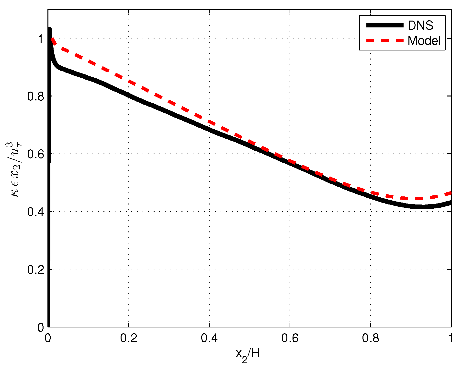
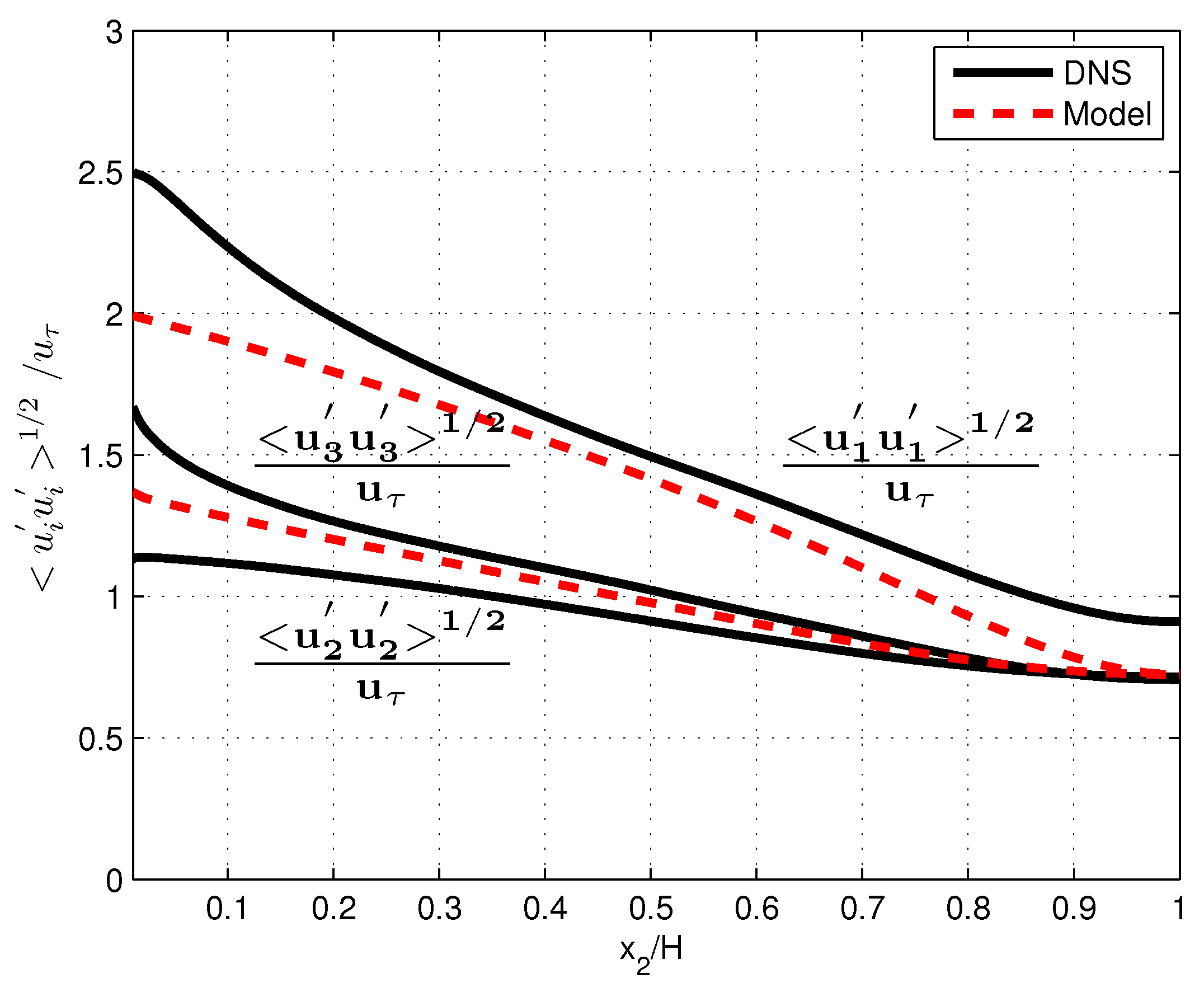
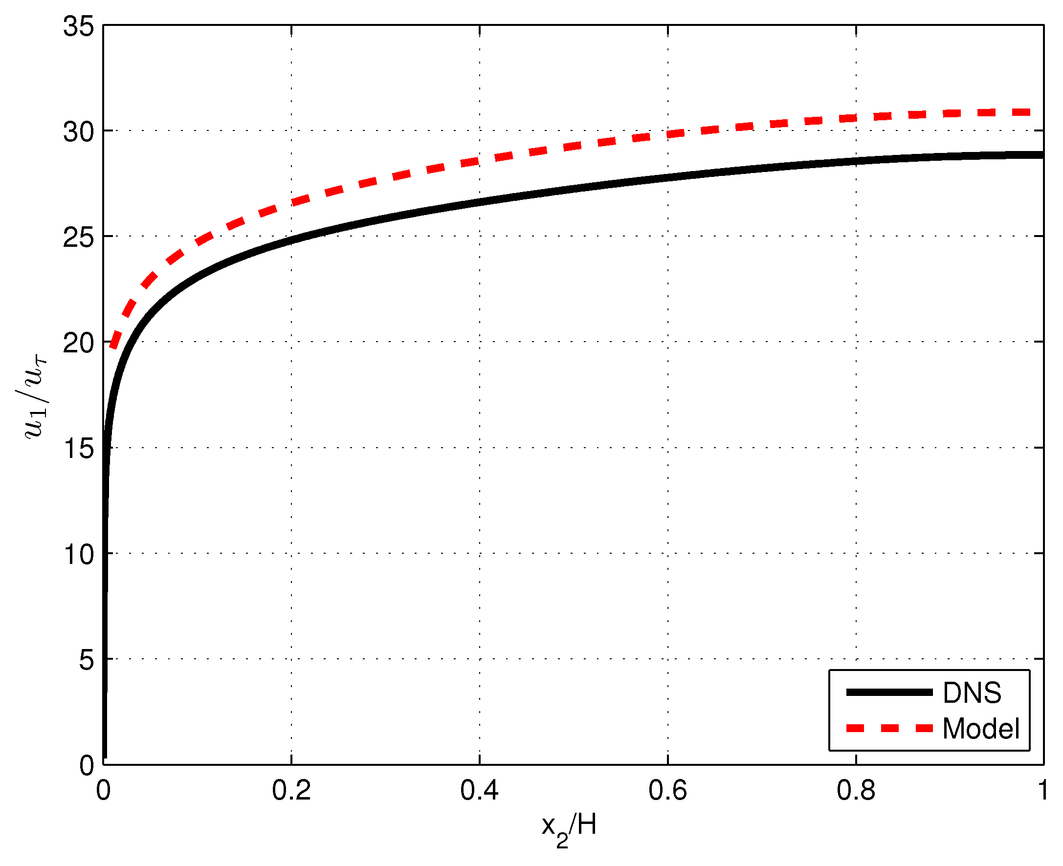
Values for k 0 and ϵ were derived by obtaining the numerical solutions of Equations (24) and (25) that were subject to the boundary conditions of Equations (26) and (27). These values were used to determine the diffusion coefficient of turbulent shear stress or viscosity D 22 , according to Equation (20); of the Reynolds stresses, according to Equations (21) and (22); and of the kinetic energy k according to Equation (23). Predictions were compared with the DNS results for R e τ = 10 4 [7]. In Figure 1 and Figure 2, kinetic energy k and the energy dissipation rate represented by G = κ ϵ x 2 are presented as a function of distance from the wall x 2 H . In Figure 3, plots are presented of the diffusion constant according to Equation (20) and turbulent viscosity ν t = < u 1 u 2 > d u 1 d x 2 according to the DNS. Figure 4 shows the distributions of the standard deviations of the three velocity fluctuations, both according to the model and the DNS. In Figure 5, mean velocities u 1 obtained through the integration of Equation (19) and obtained from the DNS are shown. Integration starts at x 2 = 100 H R e τ with a value of u 1 in accordance with its value for the boundary layer at this point. In all figures, the viscous layer at 0 < x 2 H < 0.01 is omitted.

8. Discussion of Results

Analytical expressions were given for turbulent diffusion and Reynolds stresses, describing their dependency on the gradients of mean flow. They are the result of further expanding previously published descriptions of these quantities [5] in powers of the inverse of the Kolmogorov constant C 0 while retaining the same truncation error (Section 3). Differences between the previously presented results for channel flow [5] and those of the upgraded model are limited. They are due to the direct or implicit inclusion of terms of an order higher than C 0 2 when using original Formulation (6), as was carried out in [5]; in the present upgraded model, such terms were dropped. Differences are indicative for the inaccuracy of truncation for both approaches. The advantage of the present model is that it provides a direct insight into the effect of mean flow gradients on parameters of turbulence. Moreover, implementation in a numerical code is much more easy as it circumvents the solution of complicated algebraic equations for covariances.
Predicted values of turbulent viscosity, turbulent diffusion of conservative scalars (temperature, passive admixture), and of mean velocity compare quite well with those of DNS of channel flow (Figures 3 and 5 and the results of ref. [8]). This contrasts with the predictions of the empirical basic k- ϵ model, revealing remarkable differences [5]. In the basic k- ϵ model, the turbulent diffusion coefficient is modelled by the following relation:
D i j = c μ k 2 ϵ δ i j
where c μ is a calibration constant whose value is usually set to 0.09 [1,2,3,4]. Using DNS data for k 2 ϵ , the value of the diffusion coefficient according to Equation (28) is seen to differ significantly from that of the DNS (Figures 1 and 2 of ref. [5]). Differences vary strongly with the distance from the wall, which indicates that the functional relationship according to Equation (28) is not a good representation of the turbulent diffusion of momentum [5]. It contrasts with the results of the present model. In case of channel flow, the second and third terms on the RHS of Equation (8) become zero when determining D 22 , as is seen in Equation (20). Only the isotropic part of the general expression for diffusion remains in case of D 22 . However, this isentropic representation differs from the semi-empirical model according to Equation (28). Firstly, Equation (20) does not contain a calibration factor, but it is specified by the universal Kolmogorov constant. Secondly, the value of the diffusion constant is determined by the kinetic energy associated with the isotropic state k 0 . This parameter is smaller than the kinetic energy of anisotropic flow, as follows from Equation (9), and its dependency on distance from the wall is different as well. The result supports a favourable comparison of the present model with DNS (Figure 3).
Model results for kinetic energy and energy dissipation shown in Figure 1 and Figure 2 are in satisfactory agreement with DNS. Results for the root mean squares of velocity fluctuations reveal basic trends of anisotropy (Figure 4). Deviations from DNS may be attributed to the omission of higher-order terms in the Langevin and diffusion equation, which were the origin of the present results.
The only fit factors in the model are c k and σ ϵ * , which calibrate the magnitudes of the diffusion terms in the k- ϵ equations. Their effect on statistical predictions is limited to areas where turbulent shear stresses are small, e.g., in the core of channel flow [5].

9. Conclusions

The predictions of mean values of turbulence quantities using the anisotropic k- ϵ model show good to satisfactory agreement with the results of DNS of inhomogeneous anisotropic channel flow. Since important parts of the model are general, its application to other cases of turbulence has the potential of yielding good predictions as well. The equations underlying the model enable a straightforward implementation in a CFD code, starting from the code of the basic k- ϵ model.

Funding

This research received no external funding.

Informed Consent Statement

Not applicable.

Data Availability Statement

Data are contained within the article.

Acknowledgments

H.S. Janssen is acknowledged for performing numerical calculations; G.M. Janssen is acknowledged for preparing the manuscript.

Conflicts of Interest

Author J. J. H. Brouwers was employed by the company Romico Hold.VBA. The author declares that the research was conducted in the absence of any commercial or financial relationships that could be construed as a potential conflict of interest.

References

  1. Hanjalić, K.; Launder, B. Modelling Turbulence in Engineering and the Environment: Second-Moment Routes to Closure; Cambridge University Press: Cambridge, UK, 2011. [Google Scholar]
  2. Bernard, P.S.; Wallace, J.K. Turbulent Flow: Analysis, Measurement and Prediction; Wiley: New Jersey, NJ, USA, 2002. [Google Scholar]
  3. Ansys Fluent 12.0, Theory Guide, Section 4 Turbulence, 4.4.1 Standard k-ϵ Model. Available online: https://www.afs.enea.it/ (accessed on 23 January 2009).
  4. Comsol Multiphysics, The k-ϵ Turbulence Model. Available online: https://doc.comsol.com (accessed on 16 August 2024).
  5. Brouwers, J.J.H. The Basic k-ϵ Model and a New Model Based on General Statistical Descriptions of Anisotropic Inhomogeneous Turbulence Compared with DNS of Channel Flow at High Reynolds Number. Inventions 2024, 9, 38. [Google Scholar] [CrossRef]
  6. Hoyas, S.; Jiménez, J. Scaling of the velocity fluctuations in turbulent channels up to Re_τ = 2003. Phys. Fluids 2006, 18, 011702. [Google Scholar] [CrossRef]
  7. Hoyas, S.; Oberlack, M.; Alcántara-Ávila, F.; Kraheberger, S.V.; Laux, J. Wall turbulence at high friction Reynolds numbers. Phys. Rev. Fluids 2022, 7, 014602. [Google Scholar] [CrossRef]
  8. Kuerten, J.; Brouwers, J.J.H. Lagrangian statistics of turbulent channel flow at Re_τ = 950 calculated with direct numerical simulation and Langevin models. Phys. Fluids 2013, 25, 105108. [Google Scholar] [CrossRef]
  9. Brouwers, J.J.H. Statistical Descriptions of Inhomogeneous Anisotropic Turbulence. Mathematics 2022, 10, 4619. [Google Scholar] [CrossRef]
  10. Brouwers, J.J.H. Langevin equation of a fluid particle in wall-induced turbulence. Theor. Math. Phys. 2010, 163, 677–695. [Google Scholar]
  11. Brouwers, J.J.H. Langevin and diffusion equation of turbulent fluid flow. Phys. Fluids 2010, 22, 085102. [Google Scholar] [CrossRef]
  12. Brouwers, J.J.H. Statistical description of turbulent dispersion. Phys. Rev. E Stat. Nonlinear Soft Matter Phys. 2012, 86, 066309. [Google Scholar] [CrossRef] [PubMed]
  13. Brouwers, J.J.H. Statistical Models of Large Scale Turbulent Flow. Flow Turbul. Combust. 2016, 97, 369–399. [Google Scholar] [CrossRef]
  14. van Kampen, N.G. Stochastic Processes in Physics and Chemistry, 3rd ed.; Elsevier: New York, NY, USA, 2007. [Google Scholar]
  15. Stratonovich, R.L. Topics in the Theory of Random Noise; Gordon and Breach: New York, NY, USA, 1967; Volume 1. [Google Scholar]
  16. Landau, L.D.; Lifshitz, E.M. Statistical Physics; Elsevier: Amsterdam, The Netherlands, 2007. [Google Scholar]
  17. Reichl, L.E. A Modern Course in Statistical Physics, 1st ed.; Wiley-VCH: New York, NY, USA, 2009. [Google Scholar]
  18. Fertziger, J.H.; Kaper, H.G. Mathematical Theory of Transport Processes in Gases; North-Holland Publishing Company: Amsterdam, The Netherlands; London, UK, 1972. [Google Scholar]
  19. Monin, A.S.; Yaglom, A.M. Statistical Fluid Mechanics; Dover: New York, NY, USA, 2007; Volume II, Chapter 8. [Google Scholar]
  20. Sawford, B.L.; Yeung, P.K. Lagrangian statistics in uniform shear flow: Direct numerical simulation and Lagrangian stochastic models. Phys. Fluids 2001, 13, 2627. [Google Scholar] [CrossRef]
  21. Pope, S.B. Turbulent Flows; Cambridge University Press: Cambride, UK, 2000. [Google Scholar]
  22. Thomson, D.J. Criteria for the selection of stochastic models of particle trajectories in turbulent flows. J. Fluid Mech. 1987, 180, 529. [Google Scholar] [CrossRef]
  23. Batchelor, G.K. An Introduction to Fluid Dynamics; Cambridge University Press: New York, NY, USA, 2006. [Google Scholar]
  24. Monin, A.S.; Yaglom, A.M. Statistical Fluid Mechanics; Dover: New York, NY, USA, 2007; Volume I. [Google Scholar]
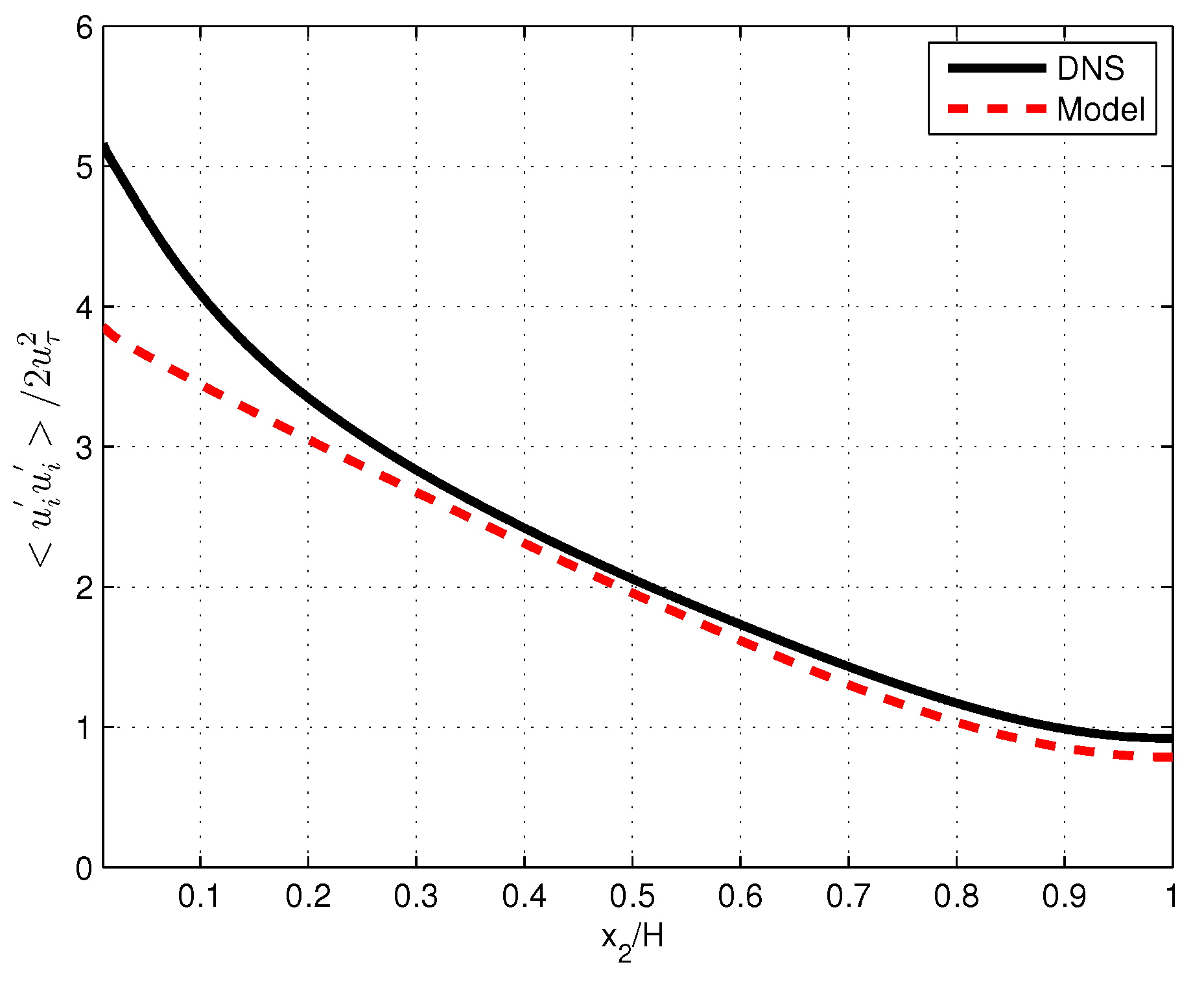
Figure 1. Dimensionless kinetic energy of fluctuations versus dimensionless distance from the channel wall ( 0.01 x 2 H 1 ) according to DNS at R e τ = 10 4 and the anisotropic model.
Inventions 09 00095 g001
Figure 2. Dimensionless and normalised energy dissipation rate versus dimensionless distance from the channel wall ( 0.01 x 2 H 1 ) according to DNS at R e τ = 10 4 and the anisotropic model.
Inventions 09 00095 g002
Figure 3. Dimensionless turbulent diffusion constant versus dimensionless distance from the channel wall ( 0.01 x 2 H 1 ) according to DNS at R e τ = 10 4 and the anisotropic model.
Inventions 09 00095 g003
Figure 4. Dimensionless standard deviations of fluctuating velocities versus dimensionless distance from the channel wall ( 0.01 x 2 H 1 ) according to DNS at R e τ = 10 4 and the anisotropic model.
Inventions 09 00095 g004
Figure 5. Dimensionless mean velocity versus dimensionless distance from the channel wall ( 0.01 x 2 H 1 ) according to DNS at R e τ = 10 4 and the anisotropic model.
Inventions 09 00095 g005
Disclaimer/Publisher’s Note: The statements, opinions and data contained in all publications are solely those of the individual author(s) and contributor(s) and not of MDPI and/or the editor(s). MDPI and/or the editor(s) disclaim responsibility for any injury to people or property resulting from any ideas, methods, instructions or products referred to in the content.