A Revision of Empirical Models of Stirling Engine Performance Using Simple Artificial Neural Networks

Abstract

Stirling engines are currently of interest due to their adaptability to a wide range of energy sources. Since simple tools are needed to guide the sizing of prototypes in preliminary studies, this paper proposes two groups of simple models to estimate the maximum power in Stirling engines with a kinematic drive mechanism. The models are based on regression or ANN techniques, using data from 34 engines over a wide range of operating conditions. To facilitate the generalisation and interpretation of results, all models are expressed by dimensionless variables. The first group models use three input variables and 23 data points for correlation construction or training purposes, while another 66 data points are used for testing. Models in the second group use eight inputs and 18 data points for correlation construction or training, while another 36 data points are used for testing. The three-input models provide estimations of the maximum brake power with an acceptable accuracy for feasibility studies. Using eight-input models, the predictions of the maximum indicated power are very accurate, while those of the maximum brake power are less accurate, but acceptable for the preliminary design stage. In general, the best results are achieved with ANN models, although they only employ one hidden layer.

1. Introduction

The oldest heat engines in use today are Stirling cycle engines. It is often emphasised that this type of cycle has the highest achievable efficiency under ideal conditions, but its greatest advantage might be the possibility of using a wide variety of energy sources, with low levels of chemical and noise pollution. Apart from refrigeration and cryogenic applications, where the Stirling cycle has achieved remarkable developments [1], technological and commercial vicissitudes over more than two hundred years have restricted the current applications of the Stirling engine practically, to cases where there is less competition. These range from anaerobic underwater equipment [2] to the combined production of heat, cooling, and electricity, especially in systems powered by waste heat [3] and renewable energies on a low power scale [4,5,6,7]. Additionally, variants of the Stirling engine are among the alternatives being evaluated for power generation in space, both for space missions and for terrestrial use [8,9].

Comparisons with other technologies are based on technical indicators, such as efficiency, mean effective pressure and specific power, as well as economic indicators. Regarding the latter, units based on Stirling engines present, in general, higher investment costs than units based on internal combustion engines, since they are not currently mass-produced, but they are economically competitive with fuel cell-based units. Their durability and relatively low maintenance costs [7] are additional strengths to the other advantages already mentioned.

The so-called Beale number is often used to estimate the specific power or mean effective pressure of a Stirling engine, not only in preliminary technical feasibility studies but also in academic analyses [10,11,12]. William Beale observed that the maximum brake power in well-developed engines is roughly proportional to the mean cycle pressure, cycle volume amplitude, and engine rotational frequency. Walker called Beale’s number, $N_B$, the proportionality constant [13]. Thus, the product of $N_B$ and the mean pressure would be approximately equal to the mean effective pressure which, multiplied by the rotational frequency, would be equal to the specific power of the engine.

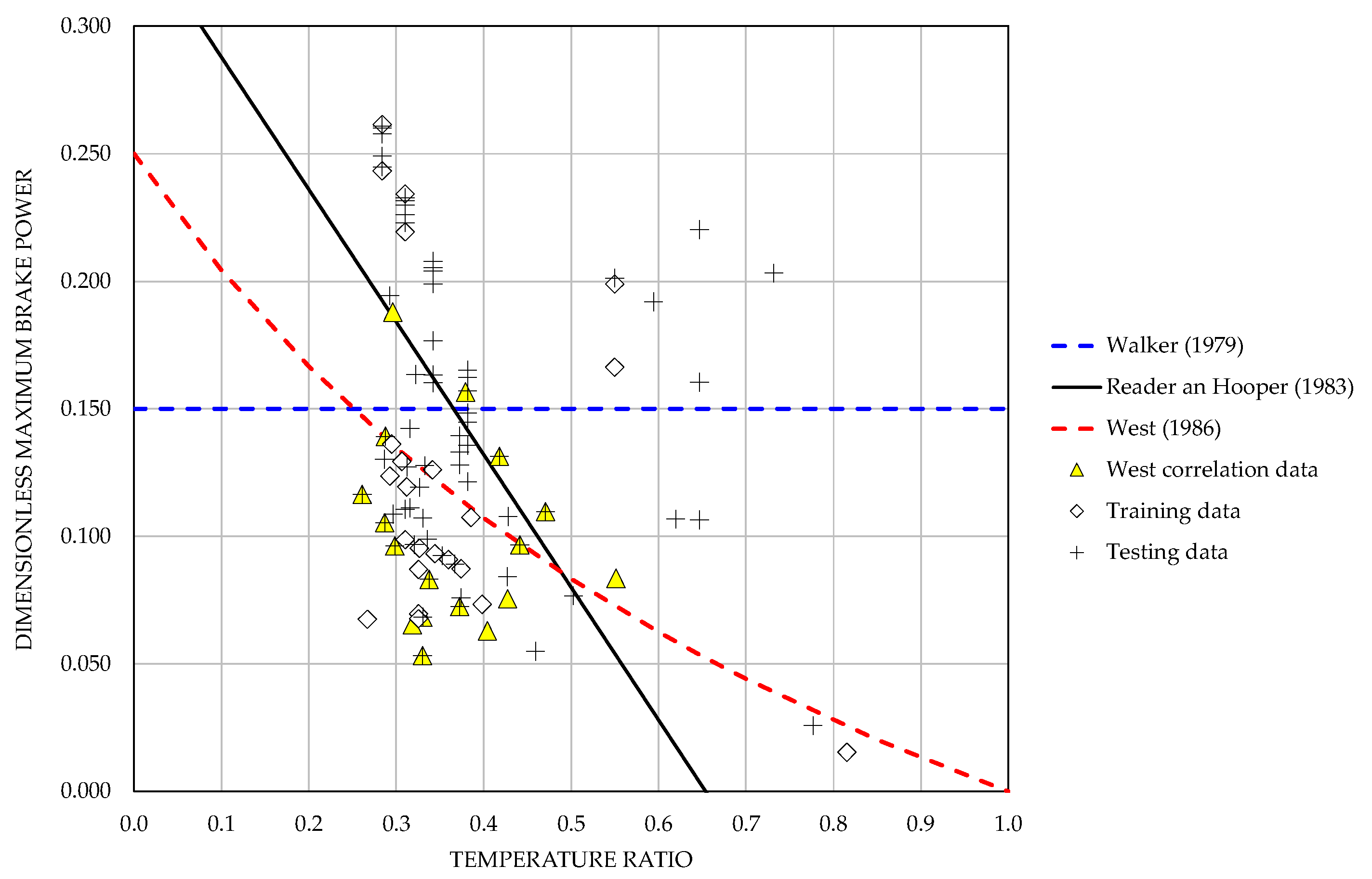
The $N_B\approx 0.15$ value was obtained from the data of 24 engines, most of them operating with a heater temperature of about 650 °C. Nonetheless, using data from 14 engines with kinematic drive mechanisms, including the original 1843 Stirling engine, and 8 free piston Stirling engines (FPSE), West [14] deduced that the assumed proportionality constant varied in the range of 0.06 to 0.23, and could be expressed as a function of the ratio of the absolute temperatures of the heater and cooler. Reader and Hooper proposed that this function was linear [15]. Other authors, using data from six operating points measured on five engines, two of them in the low temperature difference range, derived a correlation between the dimensionless maximum brake power and the main operating variables, i.e., pressure and temperatures, by a dimensional analysis [16]. The proposal has been interpreted as a variant of West’s correlation, with doubtful applicability to other engines due to the small number of parameters and influential variables considered in the model [17]. However, it should be recognised that these authors pointed out the need to obtain an additional correlation to estimate the engine speed corresponding to the maximum power.

Previously, Organ [18] and, independently, Prieto et al. [19,20], had already deduced that the dimensionless maximum indicated power is a function of more than twenty dimensionless parameters and variables, laying the foundations for the similarity of Stirling engines and the application of scaling techniques for engines with a kinematic drive mechanism [21,22]. Subsequently, Formosa and Fréchette [23] studied the similarity of FPSEs. Prieto and co-workers [24] deduced, from basic thermodynamic concepts and experimental data, that the engine speed corresponding to the maximum indicated power is not an independent variable in engines with a kinematic drive mechanism, but a function of the engine parameters and operating variables. They also analysed the leakage and mechanical losses of indicated power, and extended the model previously established for the gas circuit to the analysis of mechanical efficiency and brake power [25].

Correlations based on a few variables often lead to predictions of insufficient accuracy, even within the scope of their main objective, which is to guide the preliminary sizing of new prototypes. Therefore, correlations have been obtained based on a larger number of influential variables, using 21 operating points of eight engines, both for the dimensionless values of maximum indicated and brake power, as well as for the corresponding dimensionless speeds [26]. Although the use of dimensionless variables facilitates the generalisation of the results, and the study has recently been extended to 54 operating points of 10 engines [27], the lack of data certainly limits the applicability of the correlations for engines not included in the databases.

Recently, soft computing methods based on genetic algorithms, particle swarm optimisation, fuzzy logic, and artificial neural networks (ANN), are an alternative to regression-based correlations. Soft computing methods have, so far, mainly been applied to design or optimise particular Stirling engines, often FPSEs [28]. A smaller number of soft-computing models are known to have been developed using the databases of a set of engines. The temperature of the heat source, rotation speed, fuel, and pressure have been selected as input variables in ANN-based approaches proposed to predict the torque and brake power of a Stirling engine, using experimental data, obtained mostly from the Philips M102C engine, to test, validate, and train the model [29,30]. The temperature of the heat source, rotation speed, and type of engine configuration have given good results as input variables for other torque and brake power prediction models, which have used a larger amount of data from several engines for training, testing, and validation, but limited to the ranges of 453–1273 K, 46–1800 rpm, and 0.3–500 W [31].

The main novelties of this paper are the following:

• Two groups of models are proposed to replace the Beale, West, and similar correlations for feasibility studies and the preliminary sizing of Stirling engines with a kinematic drive mechanism, as complementary tools to more advanced procedures for analysis, design, and optimisation. The aim is to cover the widest possible diversity of size, power, and ranges of operating variables, even though this may penalise the accuracy of the model predictions. It is rare to find experimental data on Stirling engines in the literature that are extensive enough to be used reliably for model building. In addition, the stages of design, manufacture, testing, optimisation, and commercial development of a prototype are a relatively long evolutionary process, so that not many engines have progressed beyond research and demonstration phases. It is, therefore, recognised that some objectives of the article are subject to the quality of the databases used and future improvements;
• Group G1 includes models that, in combination, allow the maximum brake power to be estimated using three input variables. The G1-1R and G1-2R models are based on regression fitting techniques, while the G1-3ANN and G1-4ANN models are based on ANN methodologies. In G1 models, only the working gas, heater and cooler wall temperatures, mean pressure, and cycle volume amplitude are used as input variables. The results are evaluated using data collected from the literature for 89 operating points of 34 engines with very different characteristics, which provides a wide overview of the ranges of parameters and operating variables;
• Group G2 includes four correlations for estimating the maximum indicated and brake power, obtained by regression in a previous study [27], which are referred to in this paper as G2-5R, G2-6R, G2-7R, and G2-8R models. These correlations use eight input variables, often not available in the literature, and were, therefore, evaluated on data from a smaller number of engines. The results are compared in the article with those obtained using the new G2-9ANN, G2-10ANN, G2-11ANN, and G2-12ANN models, based on neural networks.

The use of dimensionless input and output variables allows the influence of a larger number of parameters and variables to be considered, and facilitates the generalisation of results. Comparisons between models are made in all cases using appropriate statistical indicators to highlight the advantages and limitations of each type of model.

2. Materials and Methods

2.1. Selection of Input Variables

The indicated power $P_{ind}$ developed by a Stirling engine with a kinematic drive mechanism depends on the following set of variables:

• Heater wall temperature $T_{wE}$ and cooler wall temperature $T_{wC}$;
• Mean pressure of the working gas, $p_m$;
• Phase angle $\alpha$ and other geometrical parameters of the pistons and the drive mechanism, $l_1,\dots ,l_n$, which determine the shape and volume amplitude $V_0$ of the thermodynamic cycle;
• Dead volume $V_{dx}$, wetted surface $A_{wx}$, and hydraulic radius $r_{hx}$ of each gas circuit space $x$;
• Physical properties of the working fluid, i.e., adiabatic coefficient $\gamma$, specific constant $R$, and viscosity $\mu$;
• Thermal diffusivity ${\alpha }_R$, volumetric specific heat capacity ${\rho }_R{c}_R$, and volumetric porosity ${\mathrm{\P }}_V$ of the regenerator material;
• Frequency of rotation, $n_s$.

Applying Buckingham’s theorem, with $p_m$, $V_0$, $T_{wC}$ and $n_s$ as reference variables, leads to the following equivalent functional relationship between dimensionless variables [20]:

$${\zeta }_{ind}=\mathrm{f}\left(\tau ,{\alpha ,\lambda }_1,\dots ,{\lambda }_{n-1},{\mu }_{dx},\dots ,{\alpha }_{wx},\dots ,{\lambda }_{hx},\dots ,{\mathrm{\P }}_V,\gamma ,N_p,N_{MA},N_{FO},N_{TCR}\right),$$

(1)

where ${\zeta }_{ind}=P_{ind}/\left(p_m{V}_0{n}_s\right)$, $\tau =T_{wC}/T_{wE}$, ${\lambda }_{\mathrm{i}}=l_i/V_0^{1/3}$, ${\mu }_{dx}=V_{dx}/V_0$, ${\alpha }_{wx}=A_{wx}/V_0^{2/3}$, ${\lambda }_{hx}=r_{hx}/V_0^{1/3}$, $N_p=p_m{V}_0^{1/3}/\left(\mu \sqrt{R{T}_{wC}}\right)$, $N_{MA}=n_s{V}_0^{1/3}/\sqrt{R{T}_{wC}}$, $N_{FO}={\alpha }_R/\left(n_s{V}_0^{1/3}\right)$, and $N_{TCR}={\rho }_R{c}_R{T}_{wC}/p_m$.

The characteristic Mach number $N_{MA}$ is a dimensionless velocity form representing the influence of the operating frequency $n_s$. In order to make this influence explicit, the following equation has been proposed [24]:

$${\zeta }_{ind}={\zeta }_0-\mathsf{\Phi }{N}_{MA}-\mathsf{\Psi }{N}_{MA}^2,$$

(2)

where ${\zeta }_0$ is the dimensionless quasi-static work per cycle, i.e., a theoretical limit of the gas circuit performance that, irrespective of the configuration, operating point and working fluid, cannot be reached by real engines, while the coefficients $\mathsf{\Phi }$ and $\mathsf{\Psi }$ are macroscopic representations of the indicated power losses associated with irreversibilities inherent to working gas friction and heat transfer. Depending on whether the drive mechanism is harmonic or non-harmonic, ${\zeta }_0$ can be calculated with analytical equations or by numerical simulation using, in both cases, an isothermal model of the thermodynamic cycle. Functionally, ${\zeta }_0$ depends on the temperature ratio, the parameters of the drive mechanism, and the dead volumes, but is independent of the working fluid and the mean pressure, so the following relationship can be written:

$${\zeta }_0=f\left(\tau ,{\alpha ,\lambda }_1,\dots ,{\lambda }_{n-1},{\mu }_{dx},\dots \right)$$

(3)

The following conclusions can be drawn from Equation (2) [24]:

• The dimensionless maximum indicated power, ${\zeta }_{ind,\mathrm{m}\mathrm{a}\mathrm{x}}$, must be within the following range of variation:

  $$\frac{1}{2}\le \frac{{\zeta }_{ind,\mathrm{m}\mathrm{a}\mathrm{x}}}{{\zeta }_0}\le \frac{2}{3}$$

  (4)
• The dimensionless speed corresponding to the maximum indicated power value, $N_{MA,\mathrm{m}\mathrm{a}\mathrm{x}}$, is not an independent design parameter, but a function which depends on the same parameters influencing the gas circuit performance;
• The coefficients of indicated power losses are inversely proportional to $N_{MA,\mathrm{m}\mathrm{a}\mathrm{x}}$, as the following equations show:

  $$\mathsf{\Phi }=\frac{{2{\zeta }_0-\zeta }_{ind,\mathrm{m}\mathrm{a}\mathrm{x}}}{N_{MA,\mathrm{m}\mathrm{a}\mathrm{x}}}.$$

  (5)

  $$\mathsf{\Psi }=\frac{{2\zeta }_{ind,\mathrm{m}\mathrm{a}\mathrm{x}}-{\zeta }_0}{N_{MA,\mathrm{m}\mathrm{a}\mathrm{x}}}.$$

  (6)

On the other hand, the mechanical losses of indicated power caused by leakage or friction depend on the same variables influencing the operation of the gas circuit, and on additional parameters characteristic of the seals and the drive mechanism, the influence of which can be expressed by mechanical efficiency. Therefore, the maximum brake power $P_{B,\mathrm{m}\mathrm{a}\mathrm{x}}$ depends on more than thirty parameters and operating variables.

2.1.1. Input Variables for Group G1 Models

A simplified version of Stirling engine operation is to assume that the maximum brake power $P_{B,\mathrm{m}\mathrm{a}\mathrm{x}}$ can be estimated by knowing only the main operating variables, i.e.,

$$P_{B,\mathrm{m}\mathrm{a}\mathrm{x}}\approx \mathrm{f}\left(T_{wE},T_{wC},p_m,V_0,n_{s,\mathrm{m}\mathrm{a}\mathrm{x}}^{*}\right)$$

(7)

where $n_{s,\mathrm{m}\mathrm{a}\mathrm{x}}^{*}$ is the engine speed corresponding to the peak power point.

From this expression, Buckingham’s theorem leads to the following equivalent functional relationship:

$${\zeta }_{B,\mathrm{m}\mathrm{a}\mathrm{x}}\approx \mathrm{f}\left(\tau \right)$$

(8)

where ${{\zeta }_{B,\mathrm{m}\mathrm{a}\mathrm{x}}=P}_{B,\mathrm{m}\mathrm{a}\mathrm{x}}/\left(p_m{V}_0{n}_{s,\mathrm{m}\mathrm{a}\mathrm{x}}^{*}\right)$ is the dimensionless maximum brake power.

Particular cases of this approach are the Beale, Reader and Hooper, and West correlations, which can be expressed, respectively, by the following equations:

$${\zeta }_{B,\mathrm{m}\mathrm{a}\mathrm{x}}\approx 0.15\left(\mathrm{f}\mathrm{o}\mathrm{r} \tau \approx 0.3\right)$$

(9)

$${\zeta }_{B,\mathrm{m}\mathrm{a}\mathrm{x}}\approx 0.34-0.52\tau$$

(10)

$${\zeta }_{B,\mathrm{m}\mathrm{a}\mathrm{x}}\approx 0.25\frac{1-\tau }{1+\tau }$$

(11)

For the G1 models in this article, it is assumed that $P_{B,\mathrm{m}\mathrm{a}\mathrm{x}}$ also depends on the properties of the working fluid and on the main variables of the thermodynamic cycle, i.e.,

$$P_{B,\mathrm{m}\mathrm{a}\mathrm{x}}\approx \mathrm{f}\left(\gamma ,R,T_{wE},T_{wC},p_m,V_0,n_{s,\mathrm{m}\mathrm{a}\mathrm{x}}^{*}\right)$$

(12)

from which Buckingham’s theorem leads to the following functional relationship:

$${\zeta }_{B,\mathrm{m}\mathrm{a}\mathrm{x}}\approx \mathrm{f}\left(\gamma ,\tau ,N_p\right)$$

(13)

On the other hand, since it is not possible to calculate $P_{B,\mathrm{m}\mathrm{a}\mathrm{x}}$ from ${\zeta }_{B,\mathrm{m}\mathrm{a}\mathrm{x}}$ without knowing the corresponding speed, the following functional relationship is assumed analogously:

$$n_{s,\mathrm{m}\mathrm{a}\mathrm{x}}^{*}\approx \mathrm{f}\left(\gamma ,R,T_{wE},T_{wC},p_m,V_0\right)$$

(14)

which leads to:

$$N_{MA,\mathrm{m}\mathrm{a}\mathrm{x}}^{*}\approx \mathrm{f}\left(\gamma ,\tau ,N_p\right)$$

(15)

The Rayleigh method allows Equations (13) and (15) to be expressed as follows for the G1-1R and G1-2R models, respectively:

$${\zeta }_{B,\mathrm{m}\mathrm{a}\mathrm{x}}\approx K{\gamma }^a{\tau }^b{N}_p^c$$

(16)

$$N_{MA,\mathrm{m}\mathrm{a}\mathrm{x}}^{*}\approx K^{’}{\gamma }^{a^{’}}{\tau }^{b^{’}}{N}_p^{c^{’}}$$

(17)

For the G1-3ANN and G1-4ANN models, the output variables ${\zeta }_{B,\mathrm{m}\mathrm{a}\mathrm{x}}$ and $N_{MA,\mathrm{m}\mathrm{a}\mathrm{x}}^{*}$ will be estimated from the same three input variables, i.e., $\gamma$, $\tau$ and $N_p$.

2.1.2. Input Variables for Group G2 Models

For the models of group G2, the maximum values of indicated and brake power, and their corresponding speeds, are estimated by the following functional relationships [27]:

$${\zeta }_{ind,\mathrm{m}\mathrm{a}\mathrm{x}},N_{MA,\mathrm{m}\mathrm{a}\mathrm{x}},{\zeta }_{B,\mathrm{m}\mathrm{a}\mathrm{x}},N_{MA,\mathrm{m}\mathrm{a}\mathrm{x}}^{*}\approx f\left({\zeta }_0,\gamma ,\tau ,N_p,\frac{{r_{hR}^{2}L}_R}{V_0},\sum {\mu }_{dx},{\mu }_{dxe},{\mu }_{dxc}\right)$$

(18)

Note that a large number of influencing variables are implicit in the dimensionless variables, while others have been considered to be specific to a later stage of dimensioning, e.g., hydraulic radii and wetted areas of the heater and cooler, wetted area, porosity and material properties of the regenerator, as well as characteristics parameters of the seal rings and drive mechanism.

The data analysis procedure in models G2-5R, G2-6R, G2-7R, and G2-8R is based on regression fitting using functional relationships of the following type:

$${\zeta }_{ind,\mathrm{m}\mathrm{a}\mathrm{x}},N_{MA,\mathrm{m}\mathrm{a}\mathrm{x}},{\zeta }_{B,\mathrm{m}\mathrm{a}\mathrm{x}},N_{MA,\mathrm{m}\mathrm{a}\mathrm{x}}^{*}\approx K{{\zeta }_0^a\gamma }^b{\tau }^c{N}_p^d{\left(\frac{{r_{hR}^{2}L}_R}{V_0}\right)}^e{\left(\sum {\mu }_{dx}\right)}^f{\mu }_{dxe}^g{\mu }_{dxc}^h$$

(19)

In models G2-9ANN, G2-10ANN, G2-11ANN, and G2-12ANN, the eight independent variables in Equation (19) are also used as input variables to estimate the same four output variables ${\zeta }_{ind,\mathrm{m}\mathrm{a}\mathrm{x}}$, $N_{MA,\mathrm{m}\mathrm{a}\mathrm{x}}$, ${\zeta }_{B,\mathrm{m}\mathrm{a}\mathrm{x}}$ and $N_{MA,\mathrm{m}\mathrm{a}\mathrm{x}}^{*}$.

2.2. Characteristics of Neural Networks

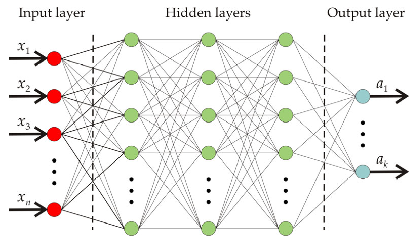
A neuron is a single cell living in a network of cells that receives inputs, processes those inputs, and generates an output [32]. Neurons can be classified into three groups or layers, as shown in Figure 1. The input layer receives the numerical data of the variables of interest $x_1,\dots ,x_n$ used to estimate the target values $a_1,\dots ,a_k$ of the network, and provides input values to the neurons that form the hidden layers of the structure, whose inputs and outputs are not accessible from outside the ANN. A neural network can have as many hidden layers as necessary, increasing the complexity of its structure, as only neurons from adjacent layers can be connected.

The output of the neurons is calculated using Equation (20). The parameter $y_j$ depicts the output value of the j-th neuron, which is calculated as the outcome of a certain activation function $f$, given a linear combination of the output values of the previous layer. Thus, $x_n$ is the input of the n-th neuron of the layer, $w_{nj}$ is the weight or gain factor of the input signals to the neuron, and $k_j$ is the independent term or offset value of each neuron. According to the literature, the activation function could be, among other options, an arctangent, the absolute value, or a ramp function [33]. The reason of this element is to introduce a non-linear component in the behaviour of the system.

$$y_j=f\left(\sum _{i=1}^n{w}_{ij}{x}_i+k_j\right)$$

(20)

Finally, the nodes of the output layer receive the outputs of the outermost hidden layer, and provide the final computation of the entire ANN. In this layer, the output of each node is calculated in the same way as in any of the previous layers. Given the structure of an ANN, even with a limited number of neurons and hidden layers, the number of variables involved in the network is large enough to make it difficult to find a direct solution to the best configuration of the network. Therefore, an optimisation or training process is required to reach the final configuration.

To carry out the training process, it is necessary to define a certain cost function and use learning algorithms, whose objective is to obtain for each neuron the weights and biases defined in Equation (20), that optimise the value of the cost function. The results are evaluated by comparing the ANN output with the target value using some statistical indicator.

There are several algorithms that can be used to optimise the network’s functioning, such as genetic or gradient algorithms. In general, no one algorithm can be considered better than another, although, depending on the characteristics of the systems, some algorithms may achieve results quicker than others, or be more appropriate for complex network configurations. In this sense, genetic algorithms are more suitable for the latter, since they are more prone to avoid getting stuck in local solutions of the cost function. In any case, the aim of this work is to analyse the feasibility of the simplest possible solution, i.e., a network with a single hidden layer and a number of neurons to be determined. Thus, a gradient algorithm is used to optimise the parameters of the ANN during the training process. However, as the whole process is based on a stochastic process, the final optimisation of the ANN may be different, depending on the algorithm used, the execution of the training process, as well as its starting point. This means that the training must be performed repeatedly until an acceptable solution is reached. Additionally, aiming to avoid an overfitting of the ANN towards the training data, optimal neuron numbers are pending further adequacy analysis, based on the results obtained for the test data.

As mentioned above, this work considers two different approaches to characterise the performance of a Stirling engine, depending on the input variables used. Consequently, two different groups of ANNs are presented, depending on the number of variables. ANN models in the G1 and G2 groups have, respectively, three and eight different nodes in the input layer, one for each input variable. To facilitate the comparison with linear regression-based models, all the networks in this paper have an output layer with a single neuron.

2.3. Experimental Data

Reasonably reliable performance data has been found for the 34 engines shown in

Table 1. Stirling engines with data analysed in this article.

No.	Engine	No.	Engine	No.	Engine
1	Mitsubishi&Daihatsu [25]	13	Ecoboy-SCM81 [25,27]	25	Philips-Ford 4-215 [14]
2	GM-GPU3 [25,26,27,34]	14	DMC-3 [35]	26	United Stirling 4-275 [14]
3	Philips MP102C [25,26,27]	15	Genoa 2 cylinder [36]	27	AIST/MITI MELSE II [14]
4	United Stirling P-40 [14,25,26,27]	16	Mitsubishi NS-03M [16]	28	Sunpower Rice husk [14]
5	SOLO V-160 [26,27,37]	17	Toshiba NS-03T [16]	29 1	JCGS System 7 [14]
6	SOLO V-161 [26,27,37]	18	Aisin Seiki NS-30A [16]	30 1	Harwell Fluidyne pump [14]
7	ST05G [27,38,39,40]	19	Sanyo NS-30S [16]	31 1	Sunpower RE-1000 [14]
8	Karabulut-1 test engine [41]	20	4-95 DA Advenco [42]	32 1	MTI TDE [14]
9	Karabulut-2 test engine [43,44]	21	STM 4-120 [42]	33 1	GE Proto-2 [14]
10	Yamanokami-2 [25,27,45]	22	Allison PD-46 [46]	34	Philips 400 HP/cyl. [27,42]
11	Kockums V4-275R Mark II [24]	23 1	Magnetic-type actuator [47]
12	Yamanokami-1 [24,27]	24	Philips 1-98 [14]

¹ Free-piston engine.

, which comprise a representative variety of existing Stirling engines.

2.3.1. Data for Analysis of Models in Group G1

Appendix A shows the 89 operating points corresponding to the engines listed in Table 1, which have been used as the basis for developing the G1-group models.

Table A1. Database of operating points for training models of group G1.

No.	Engine	Working Gas	${\mathit{V}}_0$	${\mathit{T}}_{\mathit{w}\mathit{E}}$	${\mathit{T}}_{\mathit{w}\mathit{C}}$	${\mathit{p}}_{\mathit{m}}$	${\mathit{P}}_{\mathit{B},\mathbf{m}\mathbf{a}\mathbf{x}}$	${\mathit{n}}_{\mathit{s},\mathbf{m}\mathbf{a}\mathbf{x}}^{\mathit{*}}$	${\mathit{\zeta }}_{\mathit{B},\mathbf{m}\mathbf{a}\mathbf{x}}$	${\mathit{N}}_{\mathit{M}\mathit{A},\mathbf{m}\mathbf{a}\mathbf{x}}^{\mathit{*}}$	Ref.
			(cm3)	(K)	(K)	(bar)	(W)	(rpm)
1	Mitsubishi-Daihatsu	Helium	7330.30	1173	313	108.00	44,095	495	0.0675	0.00199	[25]
2	GM GPU-3	Hydrogen	119.70	977	288	27.60	2700	3600	0.1362	0.00271	[25,26,27,34]
3	GM GPU-3	Helium	119.70	977	286	27.60	1600	2350	0.1237	0.00250	[25,26,27,34]
4	Philips MP102C	Air	64.19	1073	333	4.14	153	1475	0.2342	0.00318	[25,26,27]
5	Philips MP102C	Air	64.19	1073	333	12.41	415	1425	0.2194	0.00308	[25,26,27]
6	Philips MP102C	Air	64.19	1173	333	12.41	489	1513	0.2433	0.00327	[25,26,27]
7	Philips MP102C	Air	64.19	1173	333	4.14	184	1593	0.2615	0.00344	[25,26,27]
8	US P-40	Hydrogen	134.40	1023	333	150.00	45,245	4835	0.0696	0.00352	[25,26,27]
9	US P-40	Helium	134.40	1023	333	150.00	29,695	3265	0.0677	0.00335	[25,26,27]
10	US P-40	Nitrogen	134.40	1023	333	150.00	19,525	1670	0.0870	0.00453	[25,26,27]
11	SOLO V-160	Helium	194.55	898	336	120.00	8355	2460	0.0873	0.00284	[25,26,27,37]
12	SOLO V-160	Helium	194.55	898	323	80.00	5270	2235	0.0909	0.00263	[25,26,27,37]
13	SOLO V-160	Helium	194.55	898	309	40.00	2115	1750	0.0932	0.00211	[25,26,27,37]
14	SOLO V-161	Hydrogen	194.55	1005	328	112.20	17,860	5150	0.0953	0.00428	[25,26,27,37]
15	ST05G	Air	425.59	773	298	7.00	362	679	0.1074	0.00291	[27,39]
16	ST05G	Air	425.59	873	298	7.00	471	752	0.1261	0.00322	[27,39]
17	ST05G	Air	425.59	973	298	7.00	514	800	0.1294	0.00343	[27,39]
18	ST05G	Nitrogen	425.59	723	288	10.00	260	500	0.0733	0.00214	[27,38]
19	ST05G	Nitrogen	425.59	923	288	10.00	508	600	0.1194	0.00257	[27,38]
20	Karabulut-1	Air	231.00	533	293	1.013	13.95	215	0.1664	0.00076	[41]
21	Karabulut-2	Helium	230.00	533	293	4.00	183	600	0.1989	0.00078	[44]
22	Yamanokami-2	Air	20,106.19	368	300	7.00	670	186	0.0154	0.00287	[25,27,45]
23	Kockums V4-275R Mark II	Helium	388.91	993	308	127.00	65,000	2000	0.0987	0.00304	[24]

includes 23 operating points, corresponding to the first 11 engines listed in Table 1, operating with air, nitrogen, helium, and hydrogen, at mean pressures in the range of 1–150 bar, with heater wall temperatures ranging from 368 to 1173 K. These data have been used to build the correlations of the G1-1R and G1-2R models, and as training data for the development of the G1-3ANN and G1-4ANN models. Since the proportion of available data is not equal for all ranges of operating variables, this selection has been made to attempt to avoid bias towards any kind of engine, and to leave a significantly larger percentage of data than usual for testing purposes.

Table A2. Database of operating points for testing models of group G1.

No.	Engine	Working Gas	${\mathit{V}}_0$	${\mathit{T}}_{\mathit{w}\mathit{E}}$	${\mathit{T}}_{\mathit{w}\mathit{C}}$	${\mathit{p}}_{\mathit{m}}$	${\mathit{P}}_{\mathit{B},\mathbf{m}\mathbf{a}\mathbf{x}}$	${\mathit{n}}_{\mathit{s},\mathbf{m}\mathbf{a}\mathbf{x}}^{\mathit{*}}$	${\mathit{\zeta }}_{\mathit{B},\mathbf{m}\mathbf{a}\mathbf{x}}$	${\mathit{N}}_{\mathit{M}\mathit{A},\mathbf{m}\mathbf{a}\mathbf{x}}^{\mathit{*}}$	Ref.
			(cm3)	(K)	(K)	(bar)	(W)	(rpm)
24	Yamanokami-1	Air	25,132.74	403	313	1.00	146	1335	0.0258	0.00220	[24,25,26,27]
25	Ecoboy-SCM81	Air	81.43	703	323	8.00	59	990	0.0549	0.00235	[24,25,26,27]
26	Philips MP102C	Air	64.19	873	333	4.14	82	1120	0.1652	0.00242	[27]
27	Philips MP102C	Air	64.19	873	333	5.52	118	1229	0.1623	0.00265	[27]
28	Philips MP102C	Air	64.19	873	333	6.90	148	1274	0.1570	0.00275	[27]
29	Philips MP102C	Air	64.19	873	333	8.28	168	1280	0.1484	0.00276	[27]
30	Philips MP102C	Air	64.19	873	333	9.66	194	1299	0.1448	0.00280	[27]
31	Philips MP102C	Air	64.19	873	333	11.03	202	1265	0.1356	0.00273	[27]
32	Philips MP102C	Air	64.19	873	333	12.41	190	1178	0.1214	0.00254	[27]
33	Philips MP102C	Air	64.19	973	333	4.14	116	1288	0.2040	0.00278	[27]
34	Philips MP102C	Air	64.19	973	333	5.52	171	1392	0.2078	0.00301	[27]
35	Philips MP102C	Air	64.19	973	333	6.90	233	1966	0.1602	0.00424	[27]
36	Philips MP102C	Air	64.19	973	333	8.28	257	1411	0.2054	0.00305	[27]
37	Philips MP102C	Air	64.19	973	333	9.66	281	1368	0.1990	0.00295	[27]
38	Philips MP102C	Air	64.19	973	333	11.03	290	1393	0.1766	0.00301	[27]
39	Philips MP102C	Air	64.19	973	333	12.41	287	1324	0.1633	0.00286	[27]
40	Philips MP102C	Air	64.19	1073	333	5.52	222	1615	0.2328	0.00349	[26,27]
41	Philips MP102C	Air	64.19	1073	333	6.90	282	1650	0.2315	0.00356	[26,27]
42	Philips MP102C	Air	64.19	1073	333	8.28	333	1635	0.2299	0.00353	[26,27]
43	Philips MP102C	Air	64.19	1073	333	9.66	361	1545	0.2261	0.00334	[25,26,27]
44	Philips MP102C	Air	64.19	1073	333	11.03	392	1490	0.2230	0.00322	[26,27]
45	Philips MP102C	Air	64.19	1173	333	5.52	269	1745	0.2608	0.00377	[27]
46	Philips MP102C	Air	64.19	1173	333	6.90	340	1773	0.2602	0.00383	[27]
47	Philips MP102C	Air	64.19	1173	333	8.28	391	1710	0.2578	0.00369	[27]
48	Philips MP102C	Air	64.19	1173	333	9.66	369	1459	0.2449	0.00315	[27]
49	Philips MP102C	Air	64.19	1173	333	11.03	461	1570	0.2491	0.00339	[27]
50	SOLO V-160	Helium	194.55	898	316.4	60.00	3675	2045	0.0924	0.00243	[26,27,37]
51	SOLO V-160	Helium	194.55	898	329.8	100.00	6835	2365	0.0891	0.00276	[26,27,37]
52	GM GPU-3	Hydrogen	119.70	866	288	27.60	2110	3000	0.1277	0.00226	[25,26,27,34]
53	GM GPU-3	Hydrogen	119.70	922	288	27.60	2450	3500	0.1271	0.00264	[25,26,27,34]
54	GM GPU-3	Helium	119.70	977	286	27.60	2675	2500	0.1943	0.00266	[25,26,27,34]
55	GM GPU-3	Helium	119.70	866	286	55.20	2950	2500	0.1072	0.00266	[25,26,27,34]
56	GM GPU-3	Helium	119.70	922	286	55.20	3350	2750	0.1106	0.00293	[25,26,27,34]
57	Karabulut-2	Helium	230.00	473	293	2.80	51.93	453	0.1068	0.00059	[43]
58	Karabulut-2	Helium	230.00	453	293	1.00	38	450	0.2203	0.00059	[44]
59	Karabulut-2	Helium	230.00	453	293	2.00	61.5	500	0.1604	0.00065	[44]
60	Karabulut-2	Helium	230.00	453	293	3.00	52	425	0.1604	0.00056	[44]
61	Karabulut-2	Helium	230.00	493	293	3.00	117	530	0.1920	0.00069	[44]
62	Karabulut-2	Helium	230.00	533	293	3.00	125	540	0.2013	0.00071	[44]
63	DMC3	Air	28.65	1023	323	10.70	109	1500	0.1422	0.00251	[35]
64	Genoa 2 cyl.	Air	741.87	1023	293	15	2900	600	0.1303	0.00312	[36]
65	Mitsubishi NS-03M	Helium	161.00	971	313	62	3810	1401	0.1635	0.00157	[16]
66	Toshiba NS-03T	Helium	268.70	991	313	64	4140	1299	0.1112	0.00173	[16]
67	Aisin Seiki NS-30A	Helium	209.30	933	313	147	30,400	1500	0.0988	0.00184	[16]
68	Sanyo NS-30S	Helium	205.06	958	313	155	45,600	1805	0.1192	0.00220	[16]
69	4-95 DA Advenco	Hydrogen	134.67	1023	328	101.30	44,000	5000	0.0968	0.00367	[42]
70	STM4-120	Helium	167.19	1073	318	110	40,000	3000	0.1087	0.00339	[42]
71	Allison PD46	Helium	77.50	933	349	102	3000	3000	0.0759	0.00250	[46]
72	ST05G	Nitrogen	425.59	693	296	5.30	156	494	0.0842	0.00209	[27]
73 1	ST05G	Air	425.59	573	288	8	198	455	0.0767	0.00198	[40]
74 1	ST05G	Air	425.59	673	288	8	329	538	0.1078	0.00235	[40]
75 1	ST05G	Air	425.59	773	288	5	313	633	0.1394	0.00276	[40]
76 1	ST05G	Air	425.59	773	288	8	478	633	0.1331	0.00276	[40]
77 1	ST05G	Air	425.59	773	288	10	575	633	0.1281	0.00276	[40]
78 2	Magnetic micro-actuator	Air	0.05	373	273	1.00	0.01	600	0.2033	0.00013	[47]
79 3	Philips 1-98	Helium	98.00	1123	323	220.00	15,000	3000	0.1391	0.00281	[14]
80 3	United Stirling 4-95/P40	Hydrogen	135.00	1083	323	150.00	52,000	4000	0.0963	0.00296	[14]
81 3	Philips-Ford 4-215	Hydrogen	305.00	1023	338	200.00	125,000	4500	0.0683	0.00428	[14]
82 3	United Stirling 4-275	Helium	390.00	1123	293	150.00	118,000	2600	0.1164	0.00406	[14]
83 3	AIST/MITI MELSE II	Air	427.00	973	279	48.00	3600	1000	0.1054	0.00444	[14]
84 3	Sunpower Rice husk	Air	6900.00	793	350	5.00	4000	720	0.0966	0.00721	[14]
85 2,3	JCGS System 7	Air	0.56	773	323	18.00	5.3	2400	0.1314	0.00108	[14]
86 2,3	Harwell Fluidyne pump	Air	2320.00	633	298	1.00	14	33	0.1097	0.00025	[14]
87 2,3	Sunpower RE-1000	Air	67.00	883	298	71.00	1200	1820	0.0832	0.00421	[14]
88 2,3	MTI TDE	Air	92.00	773	288	40.00	1200	2700	0.0725	0.00707	[14]
89 2,3	GE Proto-2	Air	133.00	933	308	82.00	1750	1810	0.0532	0.00518	[14]

¹ Numerical simulation. ² Free-piston engine. ³ Used for West correlation.

includes 66 operating points, used to validate the correlations of the G1-1R and G1-2R models, and as test data for the development of the G1-3ANN and G1-4ANN models. The data correspond to 29 engines, identified in Table 1 as No. 2–5, 7–9, and 12–33, being the last 11 operating points among those used as the basis for West’s correlation. The ranges of variation of the variables used in the models of this group are probably the widest considered so far, as can be seen in

Table 2. Ranges of variables in models of group G2.

		${\mathit{V}}_0$	${\mathit{T}}_{\mathit{w}\mathit{E}}$	${\mathit{T}}_{\mathit{w}\mathit{C}}$	${\mathit{p}}_{\mathit{m}}$	${\mathit{P}}_{\mathit{B},\mathbf{m}\mathbf{a}\mathbf{x}}$	${\mathit{n}}_{\mathit{s},\mathbf{m}\mathbf{a}\mathbf{x}}^{\mathit{*}}$	$\mathit{\tau }$	$\mathit{\gamma }$	${\mathit{N}}_{\mathit{p}}$	${\mathit{\zeta }}_{\mathit{B},\mathbf{m}\mathbf{a}\mathbf{x}}$	${\mathit{N}}_{\mathit{M}\mathit{A},\mathbf{m}\mathbf{a}\mathbf{x}}^{\mathit{*}}$
		(cm3)	(K)	(K)	(bar)	(W)	(rpm)	(–)	(–)	(–)	(–)	(–)
Training data	min	64.19	533	286	1.013	1.6	186	0.267	1.40	$1.19·{10}^6$	0.0675	0.00076
	max	20,106.19	1173	336	150	65,000	5150	0.815	1.67	$1.42·{10}^8$	0.2615	0.00453
Testing data	min	0.049	373	273	1	0.01	33	0.261	1.40	$7.66·{10}^6$	0.0258	0.00013
	max	25,132.74	1173	350	220	125,000	5000	0.777	1.67	$1.16·{10}^8$	0.2608	0.00721

.

It should be noted that inconsistencies could be found in the literature regarding the volume used to express the dimensionless power developed by a Stirling engine. In general, both the symbols and the terms used may lead to confusion. For example, $V_{sw}$ is the most commonly used symbol for both the volume swept by the working piston and the amplitude of the total volume. Both values are the same for beta or gamma Stirling engines, but differ for alpha engines. To avoid ambiguity, the symbol $V_0$ is used in this article to designate the amplitude of the total volume.

2.3.2. Data for Analysis of Models in Group G2

Appendix B shows 54 operating points, corresponding to the 11 engines identified in Table 1 as No. 2–7, 10, 12, 13, and 34, which have been used as the basis for developing the G2 group models.

Table A3. Database for training G2 models [27].

No.	Engine	Working Gas	${\mathit{\zeta }}_0$	$\frac{{{\mathit{r}}_{\mathit{h}\mathit{R}}^2\mathit{L}}_{\mathit{R}}}{{\mathit{V}}_0}$	$\mathit{\gamma }$	$\sum {\mathit{\mu }}_{\mathit{d}\mathit{x}}$	${\mathit{N}}_{\mathit{p}}$	$\mathit{\tau }$	${\mathit{\mu }}_{\mathit{d}\mathit{x}\mathit{e}}$	${\mathit{\mu }}_{\mathit{d}\mathit{x}\mathit{c}}$	${\mathit{\zeta }}_{\mathit{i}\mathit{n}\mathit{d},\mathbf{m}\mathbf{a}\mathbf{x}}$	${\mathit{N}}_{\mathit{M}\mathit{A},\mathbf{m}\mathbf{a}\mathbf{x}}$	${\mathit{\zeta }}_{\mathit{B},\mathbf{m}\mathbf{a}\mathbf{x}}$	${\mathit{N}}_{\mathit{M}\mathit{A},\mathbf{m}\mathbf{a}\mathbf{x}}^{\mathit{*}}$
1	GPU3	Hydrogen	0.3121	$1.68·{10}^{-7}$	1.41	1.661	$1.43·{10}^7$	0.295	0.587	0.110	0.1554	0.00339	0.1362	0.00271
2	GPU3	Helium	0.3138	$1.68·{10}^{-7}$	1.67	1.661	$1.03·{10}^7$	0.293	0.587	0.110	0.1553	0.00309	0.1237	0.00250
3	MP102C	Air	0.4041	$1.37·{10}^{-6}$	1.40	0.776	$8.07·{10}^6$	0.310	0.088	0.088	0.2694	0.00325	0.2194	0.00308
4	MP102C	Air	0.4041	$1.37·{10}^{-6}$	1.40	0.776	$2.69·{10}^6$	0.310	0.088	0.088	0.2693	0.00340	0.2342	0.00318
5	MP102C	Air	0.4303	$1.37·{10}^{-6}$	1.40	0.776	$8.07·{10}^6$	0.284	0.088	0.088	0.2869	0.00333	0.2433	0.00327
6	MP102C	Air	0.4303	$1.37·{10}^{-6}$	1.40	0.776	$2.69·{10}^6$	0.284	0.088	0.088	0.2869	0.00360	0.2615	0.00344
7	P-40	Hydrogen	0.1833	$2.44·{10}^{-7}$	1.41	1.794	$6.77·{10}^7$	0.326	0.270	0.229	0.0997	0.00421	0.0696	0.00352
8	P-40	Helium	0.1833	$2.44·{10}^{-7}$	1.67	1.794	$4.82·{10}^7$	0.326	0.270	0.229	0.1025	0.00426	0.0677	0.00335
9	P-40	Nitrogen	0.1833	$2.44·{10}^{-7}$	1.40	1.794	$1.26·{10}^8$	0.326	0.270	0.229	0.1070	0.00524	0.0870	0.00453
10	V-161	Hydrogen	0.2019	$6.04·{10}^{-8}$	1.41	2.005	$5.83·{10}^7$	0.326	0.974	0.678	0.1088	0.00591	0.0953	0.00428
11	V-160	Helium	0.1907	$6.04·{10}^{-8}$	1.67	1.729	$4.32·{10}^7$	0.374	0.723	0.678	0.1006	0.00396	0.0873	0.00284
12	V-160	Helium	0.1975	$6.04·{10}^{-8}$	1.67	1.729	$3.02·{10}^7$	0.360	0.723	0.678	0.1045	0.00408	0.0909	0.00263
13	V-160	Helium	0.2052	$6.04·{10}^{-8}$	1.67	1.729	$1.59·{10}^7$	0.344	0.723	0.678	0.1085	0.00422	0.0932	0.00211
14	Ecoboy	Air	0.1140	$8.70·{10}^{-7}$	1.40	3.439	$5.85·{10}^6$	0.459	1.228	1.228	0.0576	0.00437	0.0481	0.00273
15	ST05G	Nitrogen	0.2662	$2.03·{10}^{-6}$	1.40	2.034	$149·{10}^7$	0.312	0.419	0.298	0.1644	0.00295	0.1194	0.00257
16	ST05G	Nitrogen	0.2183	$2.03·{10}^{-6}$	1.40	2.034	$1.49·{10}^7$	0.398	0.419	0.298	0.1322	0.00242	0.0733	0.00214
17	Yam-1	Air	0.0675	$2.49·{10}^{-9}$	1.40	2.480	$5.14·{10}^6$	0.777	1.192	1.192	0.0337	0.00269	0.0258	0.00220
18	Yam-2	Air	0.0325	$2.49·{10}^{-9}$	1.40	3.730	$3.53·{10}^7$	0.815	1.243	1.243	0.0171	0.00439	0.0154	0.00287

includes 18 operating points from nine engines, working with air, nitrogen, helium and hydrogen, at mean pressures in the range of 1–150 bar, with heater wall temperatures ranging from 403 to 1173 K. These data have been used to construct correlations for the G2-5R to G2-8R models, and as training data for the development of the G2-9ANN to G2-12ANN models.

Table A4. Database for testing G2 models [27].

No.	Engine	Working Gas	${\mathit{\zeta }}_0$	$\frac{{{\mathit{r}}_{\mathit{h}\mathit{R}}^2\mathit{L}}_{\mathit{R}}}{{\mathit{V}}_0}$	$\mathit{\gamma }$	$\sum {\mathit{\mu }}_{\mathit{d}\mathit{x}}$	${\mathit{N}}_{\mathit{p}}$	$\mathit{\tau }$	${\mathit{\mu }}_{\mathit{d}\mathit{x}\mathit{e}}$	${\mathit{\mu }}_{\mathit{d}\mathit{x}\mathit{c}}$	${\mathit{\zeta }}_{\mathit{i}\mathit{n}\mathit{d},\mathbf{m}\mathbf{a}\mathbf{x}}$	${\mathit{N}}_{\mathit{M}\mathit{A},\mathbf{m}\mathbf{a}\mathbf{x}}$	${\mathit{\zeta }}_{\mathit{B},\mathbf{m}\mathbf{a}\mathbf{x}}$	${\mathit{N}}_{\mathit{M}\mathit{A},\mathbf{m}\mathbf{a}\mathbf{x}}^{\mathit{*}}$
19	MP102C	Air	0.4041	$1.37·{10}^{-6}$	1.40	0.776	$7.17·{10}^6$	0.310	0.088	0.088	0.2698	0.00341	0.2230	0.00322
20	MP102C	Air	0.4041	$1.37·{10}^{-6}$	1.40	0.776	$6.28·{10}^6$	0.310	0.088	0.088	0.2694	0.00355	0.2261	0.00334
21	MP102C	Air	0.4041	$1.37·{10}^{-6}$	1.40	0.776	$5.38·{10}^6$	0.310	0.088	0.088	0.2698	0.00378	0.2299	0.00353
22	MP102C	Air	0.4041	$1.37·{10}^{-6}$	1.40	0.776	$4.49·{10}^6$	0.310	0.088	0.088	0.2696	0.00381	0.2315	0.00356
23	MP102C	Air	0.4041	$1.37·{10}^{-6}$	1.40	0.776	$3.59·{10}^6$	0.310	0.088	0.088	0.2697	0.00374	0.2328	0.00349
24	MP102C	Air	0.4303	$1.37·{10}^{-6}$	1.40	0.776	$7.17·{10}^6$	0.284	0.088	0.088	0.2869	0.00348	0.2491	0.00339
25	MP102C	Air	0.4303	$1.37·{10}^{-6}$	1.40	0.776	$6.28·{10}^6$	0.284	0.088	0.088	0.2815	0.00324	0.2449	0.00315
26	MP102C	Air	0.4303	$1.37·{10}^{-6}$	1.40	0.776	$5.38·{10}^6$	0.284	0.088	0.088	0.2869	0.00385	0.2578	0.00369
27	MP102C	Air	0.4303	$1.37·{10}^{-6}$	1.40	0.776	$4.49·{10}^6$	0.284	0.088	0.088	0.2869	0.00400	0.2602	0.00383
28	MP102C	Air	0.4303	$1.37·{10}^{-6}$	1.40	0.776	$3.59·{10}^6$	0.284	0.088	0.088	0.2869	0.00394	0.2608	0.00377
29	MP102C	Air	0.3745	$1.37·{10}^{-6}$	1.40	0.776	$8.07·{10}^6$	0.342	0.088	0.088	0.2170	0.00305	0.1633	0.00286
30	MP102C	Air	0.3745	$1.37·{10}^{-6}$	1.40	0.776	$7.17·{10}^6$	0.342	0.088	0.088	0.2249	0.00322	0.1766	0.00301
31	MP102C	Air	0.3745	$1.37·{10}^{-6}$	1.40	0.776	$6.28·{10}^6$	0.342	0.088	0.088	0.2455	0.00314	0.1990	0.00295
32	MP102C	Air	0.3745	$1.37·{10}^{-6}$	1.40	0.776	$5.38·{10}^6$	0.342	0.088	0.088	0.2475	0.00326	0.2054	0.00305
33	MP102C	Air	0.3745	$1.37·{10}^{-6}$	1.40	0.776	$4.49·{10}^6$	0.342	0.088	0.088	0.1884	0.00496	0.1602	0.00424
34	MP102C	Air	0.3745	$1.37·{10}^{-6}$	1.40	0.776	$3.59·{10}^6$	0.342	0.088	0.088	0.2443	0.00325	0.2078	0.00301
35	MP102C	Air	0.3745	$1.37·{10}^{-6}$	1.40	0.776	$2.69·{10}^6$	0.342	0.088	0.088	0.2386	0.00302	0.2040	0.00278
36	MP102C	Air	0.3406	$1.37·{10}^{-6}$	1.40	0.776	$8.07·{10}^6$	0.381	0.088	0.088	0.2123	0.00261	0.1214	0.00254
37	MP102C	Air	0.3406	$1.37·{10}^{-6}$	1.40	0.776	$7.17·{10}^6$	0.381	0.088	0.088	0.2139	0.00282	0.1356	0.00273
38	MP102C	Air	0.3406	$1.37·{10}^{-6}$	1.40	0.776	$6.28·{10}^6$	0.381	0.088	0.088	0.2134	0.00292	0.1448	0.00280
39	MP102C	Air	0.3406	$1.37·{10}^{-6}$	1.40	0.776	$5.38·{10}^6$	0.381	0.088	0.088	0.2095	0.00292	0.1484	0.00276
40	MP102C	Air	0.3406	$1.37·{10}^{-6}$	1.40	0.776	$4.49·{10}^6$	0.381	0.088	0.088	0.2093	0.00296	0.1570	0.00275
41	MP102C	Air	0.3406	$1.37·{10}^{-6}$	1.40	0.776	$3.59·{10}^6$	0.381	0.088	0.088	0.2076	0.00291	0.1623	0.00265
42	MP102C	Air	0.3406	$1.37·{10}^{-6}$	1.40	0.776	$2.69·{10}^6$	0.381	0.088	0.088	0.2055	0.00269	0.1652	0.00242
43	V-160	Helium	0.1940	$6.04·{10}^{-8}$	1.67	1.729	$3.68·{10}^7$	0.367	0.723	0.678	0.1024	0.00402	0.0891	0.00276
44	V-160	Helium	0.2011	$6.04·{10}^{-8}$	1.67	1.729	$2.32·{10}^7$	0.352	0.723	0.678	0.1063	0.00414	0.0924	0.00243
45	ST05G	Nitrogen	0.2038	$2.03·{10}^{-6}$	1.40	2.034	$7.59·{10}^6$	0.427	0.419	0.298	--	--	0.0842	0.00209
46	ST05G	Air	0.2250	$2.03·{10}^{-6}$	1.40	2.034	$9.84·{10}^6$	0.386	0.419	0.298	--	--	0.1074	0.00291
47	ST05G	Air	0.2491	$2.03·{10}^{-6}$	1.40	2.034	$9.84·{10}^6$	0.341	0.419	0.298	--	--	0.1261	0.00322
48	ST05G	Air	0.2697	$2.03·{10}^{-6}$	1.40	2.034	$9.84·{10}^6$	0.306	0.419	0.298	--	--	0.1294	0.00343
49 1	ST05G	Air	0.2319	$2.03·{10}^{-6}$	1.40	2.034	$1.47·{10}^7$	0.373	0.419	0.298	--	--	0.1281	0.00276
50 1	ST05G	Air	0.2319	$2.03·{10}^{-6}$	1.40	2.034	$1.17·{10}^7$	0.373	0.419	0.298	--	--	0.1331	0.00276
51 1	ST05G	Air	0.2319	$2.03·{10}^{-6}$	1.40	2.034	$7.34·{10}^6$	0.373	0.419	0.298	--	--	0.1394	0.00276
52 1	ST05G	Air	0.2034	$2.03·{10}^{-6}$	1.40	2.034	$1.17·{10}^7$	0.428	0.419	0.298	--	--	0.1078	0.00235
53 1	ST05G	Air	0.1685	$2.03·{10}^{-6}$	1.40	2.034	$1.17·{10}^7$	0.503	0.419	0.298	--	--	0.0767	0.00198
54	P400 HP/cyl.	Helium	0.4310	$1.19·{10}^{-8}$	1.67	0.749	$1.91·{10}^8$	0.313	0.280	0.111	0.2221	0.00275	0.2160	0.00232

¹ Numerical simulation.

includes 36 operating points from four engines, which have been used to validate the correlations of the G2-5R to G2-8R models, and as testing data for the development of the G2-9ANN to G2-12ANN models.

Table 3. Ranges of ordinary variables in models of group G2.

		${\mathit{V}}_0$	${\mathit{T}}_{\mathit{w}\mathit{E}}$	${\mathit{T}}_{\mathit{w}\mathit{C}}$	${\mathit{p}}_{\mathit{m}}$	${\mathit{r}}_{\mathit{h}\mathit{R}}$	${\mathit{L}}_{\mathit{R}}$	${\mathit{P}}_{\mathit{i}\mathit{n}\mathit{d},\mathbf{m}\mathbf{a}\mathbf{x}}$	${\mathit{n}}_{\mathit{s},\mathbf{m}\mathbf{a}\mathbf{x}}$	${\mathit{P}}_{\mathit{B},\mathbf{m}\mathbf{a}\mathbf{x}}$	${\mathit{n}}_{\mathit{s},\mathbf{m}\mathbf{a}\mathbf{x}}^{\mathit{*}}$
		(cm3)	(K)	(K)	(bar)	(mm)	(mm)	(W)	(W)	(W)	(rpm)
Training data	min	64.19	368	286	1	0.020	20.0	115	165	60	135
	max	25,132.74	1173	336	150	0.124	56.3	77,365	7120	45,245	5150
Testing data	min	64.19	771	303	4.1	0.020	28.0	113	532	82	448
	max	15,000	1173	333	110	0.056	75.0	325,020	3480	266,433	2365

and

Table 4. Ranges of dimensionless variables in models of group G2.

		${\mathit{\zeta }}_0$	$\frac{{{\mathit{r}}_{\mathit{h}\mathit{R}}^2\mathit{L}}_{\mathit{R}}}{{\mathit{V}}_0}$	$\mathit{\gamma }$	$\sum {\mathit{\mu }}_{\mathit{d}\mathit{x}}$	${\mathit{N}}_{\mathit{p}}$	$\mathit{\tau }$	${\mathit{\mu }}_{\mathit{d}\mathit{e}}$	${\mathit{\mu }}_{\mathit{d}\mathit{c}}$	${\mathit{\zeta }}_{\mathit{i}\mathit{n}\mathit{d},\mathbf{m}\mathbf{a}\mathbf{x}}$	${\mathit{N}}_{\mathit{M}\mathit{A},\mathbf{m}\mathbf{a}\mathbf{x}}$	${\mathit{\zeta }}_{\mathit{B},\mathbf{m}\mathbf{a}\mathbf{x}}$	${\mathit{N}}_{\mathit{M}\mathit{A},\mathbf{m}\mathbf{a}\mathbf{x}}^{\mathit{*}}$
Training data	min	0.0325	$2.487·{10}^{-9}$	1.40	0.776	$2.69·{10}^6$	0.267	0.088	0.088	0.0171	0.00242	0.0154	0.00211
	max	0.4303	$2.034·{10}^{-6}$	1.67	3.730	$1.26·{10}^8$	0.815	1.243	1.243	0.2869	0.00591	0.2615	0.00453
Testing data	min	0.1685	$1.191·{10}^{-8}$	1.40	0.749	$2.69·{10}^6$	0.261	0.088	0.088	0.1024	0.00269	0.0891	0.00198
	max	0.4310	$1.368·{10}^{-6}$	1.67	2.034	$1.91·{10}^8$	0.777	0.723	0.678	0.2869	0.00496	0.2608	0.00424

show the ranges of the variables used in the models.

2.4. Statistical Indicators

Various criteria have been proposed to assess the fit between the experimental data and model estimates, but none of them is free of limitations [48]. Since the percentage results facilitate interpretations, in this article, the performance of the models is assessed using dimensionless statistical indicators, namely the relative root mean square error RRMSE, the relative mean bias error RMBE, and the coefficient of determination $R^2$. The RRMSE value is used as an optimisation criterion for both least squares regression-based models, and for training ANN-based models. To facilitate comparisons with results from other authors, the Nash–Sutcliffe coefficient of model efficiency, NSE, and the normalised values of the root mean square error and mean bias error, NRMSE and NMBE, respectively, have also been calculated, using the mean values of the experimental data as references for the latter two. $R^2$ values range from 0 to 1, and NSE values range from −∞ to 1. Negative NSE values suggest that the mean of the measurements is a better predictor than the model estimates themselves [49]. Some authors warn against the risk of identifying the meaning of $R^2$ and NSE [50], while others try to avoid confusion by classifying the former as an indicator of dispersion and the latter as an indicator of overall performance [51]. For example, while $R^2=0.8$ indicates that the model explains 80% of the variance in the observed data, the value $NSE=0.8$ has a very different meaning, i.e., that the model mean squared error represents 20% of the observed variance. The cause of possible confusion may be that $R^2$ can be interpreted as a maximum potential value for NSE, as the following equation reduces to ${NSE=R}^2$ for the optimal case of $\stackrel{-}{s_i}=\stackrel{-}{o_i}$ and ${\sigma }_{sn}=R$ [49]:

$$NSE=2{\sigma }_{sn}R-{\sigma }_{sn}^2-{\left(\frac{\stackrel{-}{s_i}-\stackrel{-}{o_i}}{{\sigma }_o}\right)}^2$$

(21)

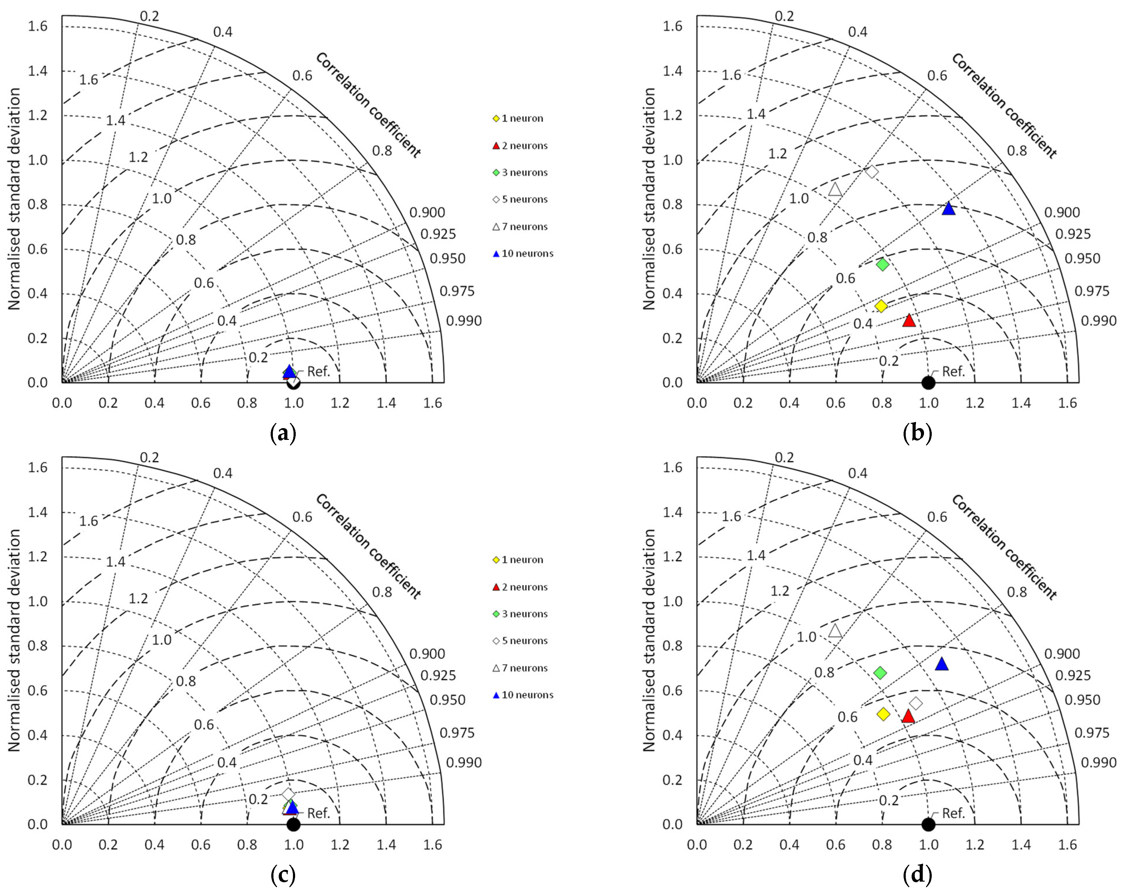
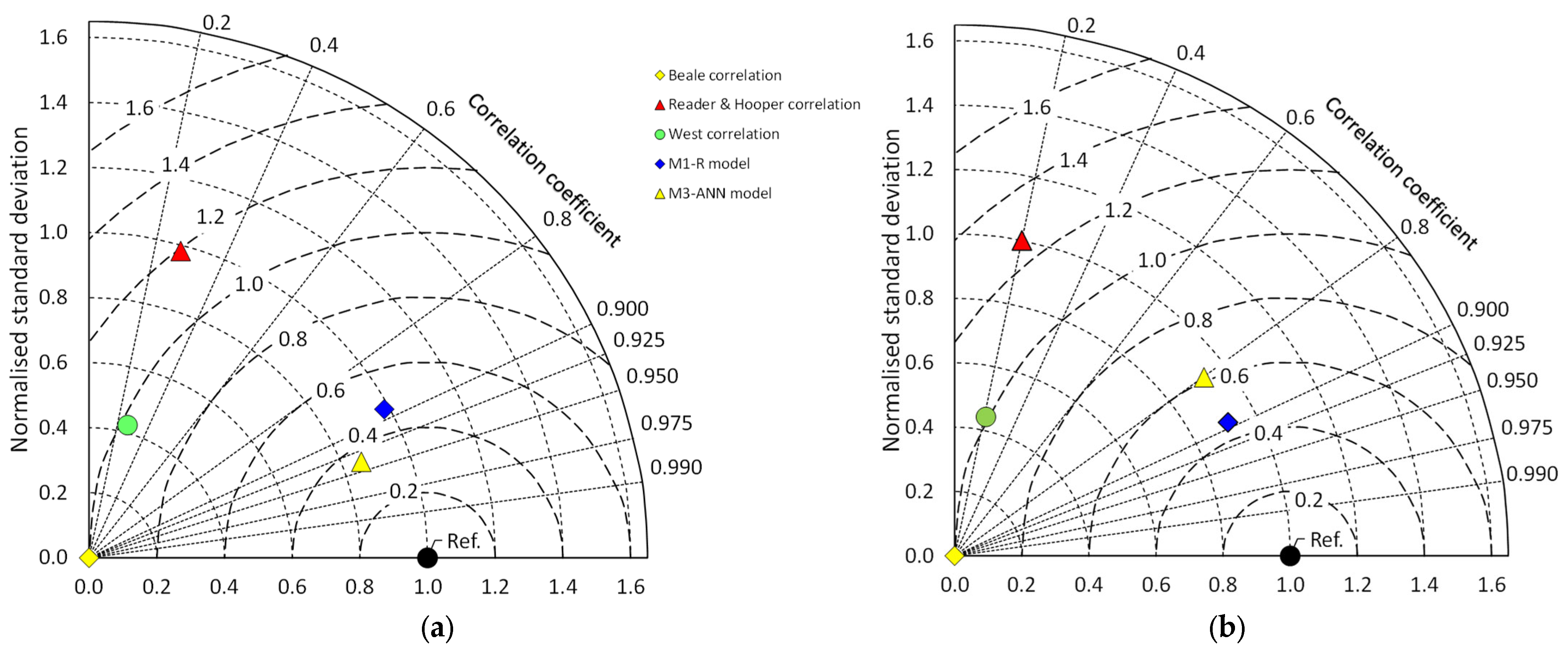
Taylor diagrams have been recommended for visualising results in model analyses [52]. In this article, this type of chart is used as an alternative to the usual scatterplots, because it provides a concise statistical summary of how well patterns match each other in terms of their correlation, their root-mean-square difference, and the ratio of their variances. The Taylor diagram is based on the definition of the centred pattern RMS difference $E^{\prime }$ [52], which is related to key statistical indicators by means of the following equations:

$$RMSE={\left(\stackrel{-}{s_i}-\stackrel{-}{o_i}\right)}^2+E^{\prime 2}$$

(22)

$$E_n^{\prime }=\sqrt{1+{\sigma }_{sn}^2-2{\sigma }_{sn}R}$$

(23)

Equation (22) and the law of cosines are the basis for the graphical representation of the degree of closeness between a model and the reference data set, using dimensionless variables (Figure 2).

3. Results

3.1. Regression-Based Models of Group G1

Figure 3 provides a picture of the dispersion between the 89 dimensionless maximum brake power data points included in Table A1 and Table A2, and the predictions based on Equations (9)–(11).

Based on Equation (13), the following correlation has been obtained, which fits the 23 operating points included in Table A1 with RRMSE = 22.2% and $R^2=0.$7847:

$${\zeta }_{B,\mathrm{m}\mathrm{a}\mathrm{x}}=7.645{\gamma }^{-0.028}{\tau }^{-1.621}{N}_p^{-0.357}$$

(24)

This equation fits the 89 operating points included in both Table A1 and Table A2 with RRMSE = 22.2% and $R^2=0.$7940. Figure 4 facilitates comparisons between data and model predictions.

Based on Equation (15), the following correlation has been obtained, which fits the 23 operating points included in Table A1 with RRMSE = 30.1% and $R^2=0.$9569:

$$N_{MA,\mathrm{m}\mathrm{a}\mathrm{x}}^{*}=0.0001682{\gamma }^{-2.305}{\tau }^{-0.780}{N}_p^{0.172}$$

(25)

This equation fits, with RRMSE = 25.3% and $R^2=0.9598$, the 82 total operating points that result after excluding the FPSE data, because of their different operating principle, and operating point No. 84, because its $N_{MA,\mathrm{m}\mathrm{a}\mathrm{x}}^{*}$ value is significantly higher than those known for engines with a kinematic drive mechanism, from Table A1 and Table A2. Figure 5 facilitates comparisons between data and model predictions.

3.2. ANN-Based Models of Group G1

The optimal number of neurons in the hidden layer is usually determined statistically by some variant of the mean square error and the coefficient of determination [53]. In this paper, the optimisation is based on RRMSE and $R^2$, whose weighting is obtained by the normalised centred pattern RMSE, $E_n^{’}$.

Table 5. Statistical results during training for ANN-based models in group G1 as a function of the number of neurons in the hidden layer.

	Neurons	1	2	3	5	7	10	12	15
G1-3ANN	RRMSE (%)	30.31	27.72	29.94	26.41	14.84	19.69	30.11	19.69
	$R^2$	0.5527	0.6345	0.4026	0.6286	0.8820	0.7402	0.3944	0.7402
	$E_n^{’}$ (%)	67.67	60.51	79.32	61.15	35.32	50.99	78.55	50.99
G1-4ANN 1	RRMSE (%)	23.80	15.81	22.49	16.89	12.47	12.82	17.00	20.36
	$R^2$	0.5264	0.7774	0.5022	0.6250	0.8386	0.8738	0.6378	0.5795
	$E_n^{’}$ (%)	75.81	50.21	74.66	61.54	41.67	38.66	60.54	78.26

¹ Excluding FPSEs and Sunbird Rice Husk engine.

and Figure 6 show that the optimal number corresponds to 7 and 10 neurons for the G1-3ANN and G1-4ANN models, respectively. In addition, Figure 7 allows comparisons to be made between the data and the predictions of the models configured with the optimal number of neurons.

3.3. Regression-Based Models of Group G2

Model G2-5R is based on the following equation, which fits the 18 available experimental data points with RRMSE = 3.20% and RMBE = −0.17%:

$${\zeta }_{ind,\mathrm{m}\mathrm{a}\mathrm{x}}=0.8280{{\zeta }_0^{1.0716}\left(\frac{{r_{hR}^{2}L}_R}{V_0}\right)}^{0.0209}{\gamma }^{-0.1696}{\left(\sum {\mu }_{dx}\right)}^{-0.0527}{N}_p^{0.0184}{\tau }^{0.1932}{{\mu }_{dxe}^{-0.1012}\mu }_{dxc}^{0.0518}$$

(26)

Figure 8 facilitates comparisons between data and model predictions.

Model G2-6R is based on the following equation, which fits the 18 experimental data points with RRMSE = 6.35% and RMBE = 0.43%:

$$N_{MA,\mathrm{m}\mathrm{a}\mathrm{x}}=0.000356{{\zeta }_0^{-2.0664}\left(\frac{{r_{hR}^{2}L}_R}{V_0}\right)}^{0.1131}{\gamma }^{-0.8828}{\left(\sum {\mu }_{dx}\right)}^{-1.8519}{N}_p^{-0.0106}{\tau }^{-2.7810}{\mu }_{dxe}^{0.5639}{\mu }_{dxc}^{0.0189}$$

(27)

Figure 9 facilitates comparisons between data and model predictions.

Model G2-7R is based on the following equation, which fits the 18 experimental data points with RRMSE = 6.39% and RMBE = −0.44%:

$${\zeta }_{B,\mathrm{m}\mathrm{a}\mathrm{x}}=0.8358{{\zeta }_0^{-0.2918}\left(\frac{{r_{hR}^{2}L}_R}{V_0}\right)}^{0.1123}{\gamma }^{-0.7655}{\left(\sum {\mu }_{dx}\right)}^{-1.6930}{N}_p^{-0.0406}{\tau }^{-1.2756}{\mu }_{dxe}^{0.4952}{\mu }_{dxc}^{-0.0429}$$

(28)

Figure 10 facilitates comparisons between data and model predictions.

Model G2-8R is based on the following equation, which fits the 18 experimental data points with RRMSE = 10.93% and RMBE = −5.15%:

$$N_{MA,max}^{*}\approx 0.000220{{\zeta }_0^{-1.0846}\left(\frac{{r_{hR}^{2}L}_R}{V_0}\right)}^{0.0322}{\gamma }^{-1.5436}{\left(\sum {\mu }_{dx}\right)}^{-0.9204}{N}_p^{0.0500}{\tau }^{-1.6547}{{\mu }_{dxe}^{0.1708}\mu }_{dxc}^{-0.0178}$$

(29)

Figure 11 facilitates comparisons between data and model predictions.

3.4. ANN-Based Models of Group G2

Table 6. Statistical results as a function of the number of neurons during training for ANN-based models in group G2.

	Neurons	1	2	3	5	7	10
G2-9ANN	RRMSE (%)	3.15	3.13	3.13	0.55	3.80	3.80
	$R^2$	0.9978	0.9979	0.9979	0.9999	0.9971	0.9970
	$E_n^{\prime }$ (%)	4.97	4.77	4.77	0.90	5.59	5.67
G2-10ANN	RRMSE (%)	7.13	7.34	10.88	20.01	16.89	21.71
	$R^2$	0.8421	0.9131	0.6948	0.3886	0.3196	0.6574
	$E_n^{\prime }$ (%)	40.06	29.48	56.72	97.92	95.95	78.96
G2-11ANN	RRMSE (%)	3.69	3.68	4.60	4.60	5.19	3.70
	$R^2$	0.9944	0.9944	0.9925	0.9810	0.9936	0.9935
	$E_n^{’}$ (%)	7.57	7.54	8.68	13.77	8.12	8.06
G2-12ANN	RRMSE (%)	10.07	8.68	15.62	13.37	16.89	17.75
	$R^2$	0.7259	0.7767	0.5754	0.7521	0.3196	0.6817
	$E_n^{’}$ (%)	53.18	49.71	71.09	54.57	51.57	72.47

and Figure 12 allow the selection of optimal neuron numbers for the G2-9ANN to G2-12ANN models, while Figure 13 provides comparisons between the data and the predictions of the models with optimal neuron numbers.

4. Discussion and Future Work

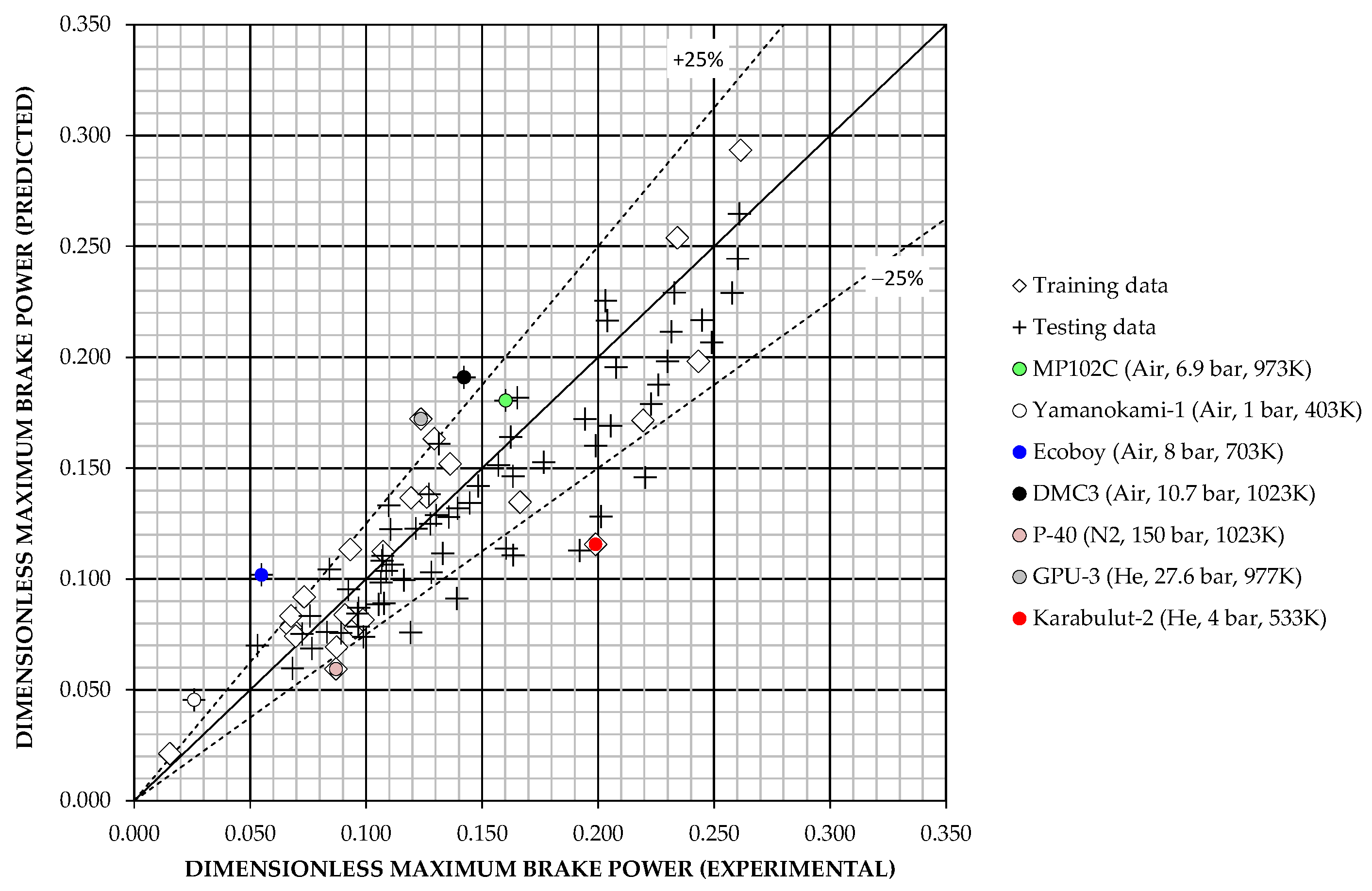
The ability of a model to accurately predict the performance of a set of Stirling engines depends on the influence between the input and output variables of the model, the representativeness and quality of the data sample used for training and testing, and the mathematical procedure of the model. High accuracy cannot be expected from the models in group G1, because they only use three input variables, although they are undoubtedly influential on the outputs. 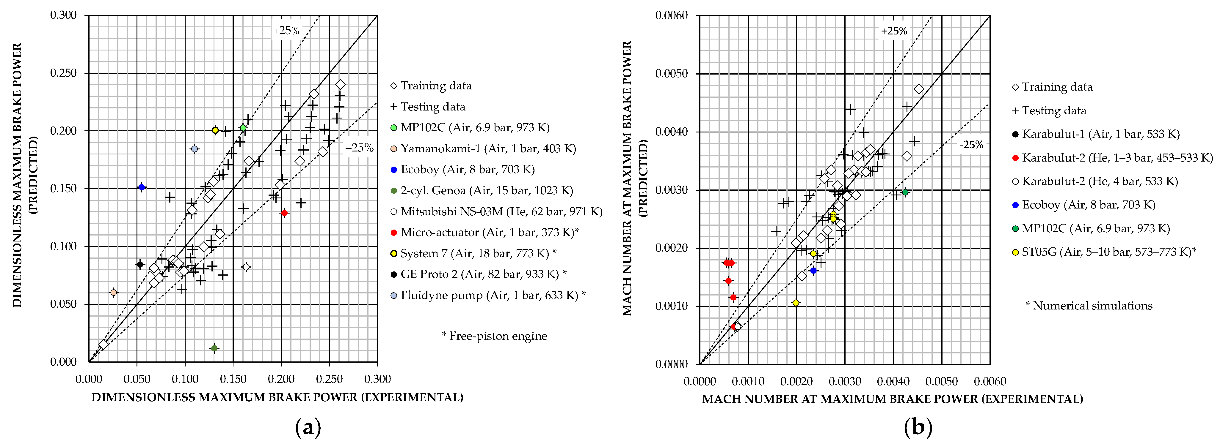Consistent with these observations, it follows from Figure 3, Figure 4 and Figure 7a that the G1-1R and G1-3ANN models are able to estimate ${\zeta }_{B,\mathrm{m}\mathrm{a}\mathrm{x}}$ with relative errors within ±25% for most of the Appendix A operating points, while the classical correlations are not adequate for a significant number of data.

Table 7. Statistical indicators of the performance of the ${\zeta }_{B,\mathrm{m}\mathrm{a}\mathrm{x}}$ models of group G1.

		RRMSE (%)	NRMSE (%)	RMBE (%)	NMBE (%)	NSE	${\mathit{R}}^2$	${\mathit{\sigma }}_{\mathit{s}\mathit{n}}$	${\mathit{E}}_{\mathit{n}}^{\mathit{\prime }}$ (%)
Training data	Beale correlation	193.01	53.28	72.56	18.49	−0.1370	0.0397	0.0000	100.00
	West correlation	49.44	49.15	14.42	−6.26	0.0324	0.0720	0.4232	97.57
	Reader and Hooper	156.88	62.45	17.41	18.71	−0.5622	0.0761	0.9817	119.25
	G1-1R	22.18	23.74	2.54	−1.27	0.7743	0.7847	0.9849	47.44
	G1-3ANN	14.84	18.37	−2.2	−5.13	0.8647	0.8820	0.8572	35.31
All data	Beale correlation	120.03	42.79	37.65	6.13	−0.0209	0.0173	0.0000	100.00
	West correlation	44.03	46.46	−2.80	−18.22	−0.1924	0.0388	0.0444	100.45
	Reader and Hooper	102.50	53.85	10.54	1.99	−0.6019	0.0401	1.0002	126.48
	G1-1R	22.15	20.21	−2.64	−6.32	0.7710	0.7940	0.9141	45.45
	G1-3ANN	34.74	26.47	−0.53	−5.76	0.6072	0.6417	0.9275	61.17

and Figure 14 facilitate comparisons using statistical indicators.

With respect to particular operating points, for the G1-1R model, the largest percentage deviations are observed for the Ecoboy and Yamanokami-1 engines and, to a lesser extent, for the Karabulut-2 engine. It is interesting to note that this model predicts ${\zeta }_{B,\mathrm{m}\mathrm{a}\mathrm{x}}$ acceptably for the FPSE analysed, including the magnetic micro-actuator of only 10 mW and 0.05 cm³, values that are well outside the range of operating points used to build the model. The G1-3ANN model fits the training data somewhat better, but is less accurate for the testing data. The largest percentage deviations are observed for the Ecoboy engine, for several FPSEs and, especially, for the 2-cylinder Genoa engine.

Regarding G1-model estimates of $N_{MA,\mathrm{m}\mathrm{a}\mathrm{x}}^{*}$, it is clear from Figure 5 that the G1-2R model gives results with relative errors within ±25% for most of the data, after excluding the FPSEs and Sunpower’s Rice Husk engine, as mentioned before. The largest percentage deviations are observed for the Mitsubishi&Daihatsu and Karabulut-1 engines and, to a lesser extent, for several operating points of the Karabulut-2 engine, and for the point No. 35 of the MP102C engine in Table A2, previously associated with a measurement error [27]. The estimates of the G1-4ANN model with 10 neurons in the hidden layer are acceptable for the training data, but worse for the testing ones, due to high percentage deviations for several operating points at low values of $N_{MA,\mathrm{m}\mathrm{a}\mathrm{x}}^{*}$, as shown in Figure 7b. However, it should be noted that such low values of $N_{MA,\mathrm{m}\mathrm{a}\mathrm{x}}^{*}$ indicate that the degree of development of the gas circuit of the corresponding engines can be improved [24], i.e., the coefficients of indicated power losses are high, as can be seen from Equations (5) and (6).

Table 8. Statistical indicators of the performance of the $N_{MA,\mathrm{m}\mathrm{a}\mathrm{x}}^{*}$ models of group G1.

		RRMSE (%)	NRMSE (%)	RMBE (%)	NMBE (%)	NSE	${\mathit{R}}^2$	${\mathit{\sigma }}_{\mathit{s}\mathit{n}}$	${\mathit{E}}_{\mathit{n}}^{\mathit{\prime }}$ (%)
Training data	G1-2R 1	30.09	21.72	3.60	−1.86	0.9569	0.9569	0.9792	20.77
	G1-4ANN 1	12.82	11.91	−1.67	−0.66	0.8504	0.8738	1.0873	38.66
All data 1	G1-2R 1	25.28	21.34	−0.31	−4.64	0.9590	0.9598	0.9510	20.25
	G1-4ANN 1	44.80	19.03	8.73	0.64	0.6729	0.6832	0.9261	57.16

¹ Excluding FPSEs and Sunbird Rice Husk engine.

shows the statistical indicators obtained for both G1-2R and G1-4ANN models.

In summary, in group G1, the proposed regression-based models are slightly better than the ANN-based models, with balanced relative errors for the total training and test data in Appendix A.

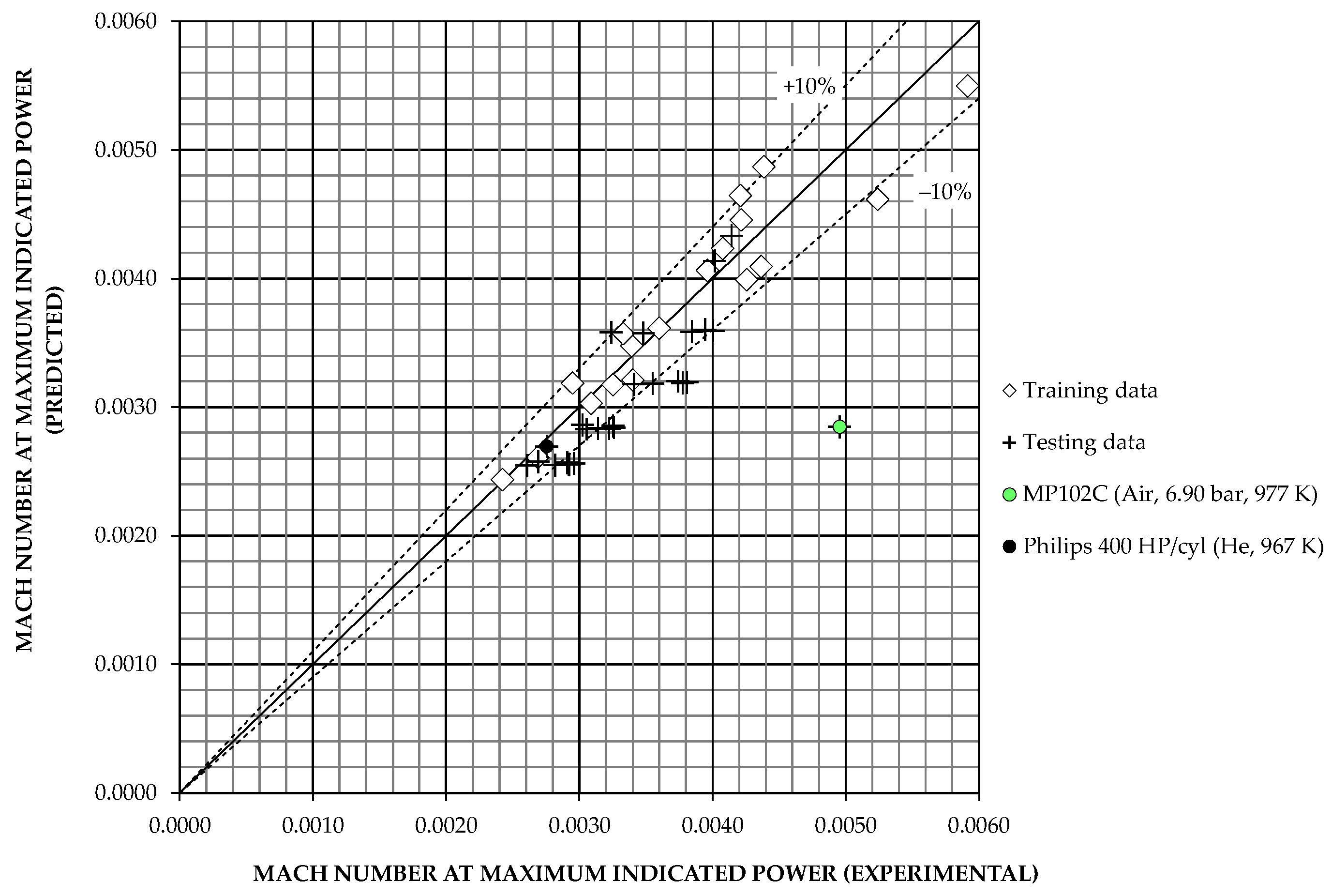
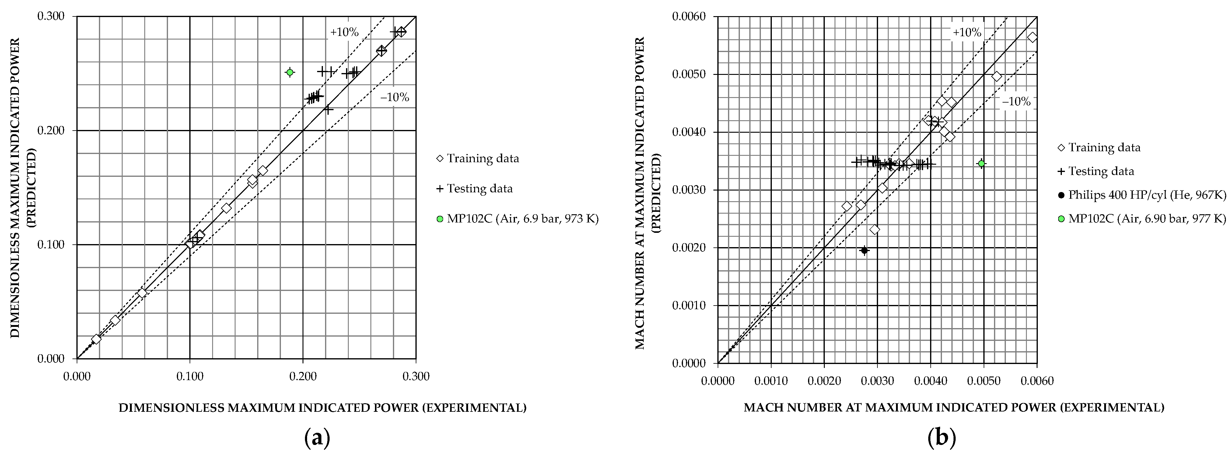
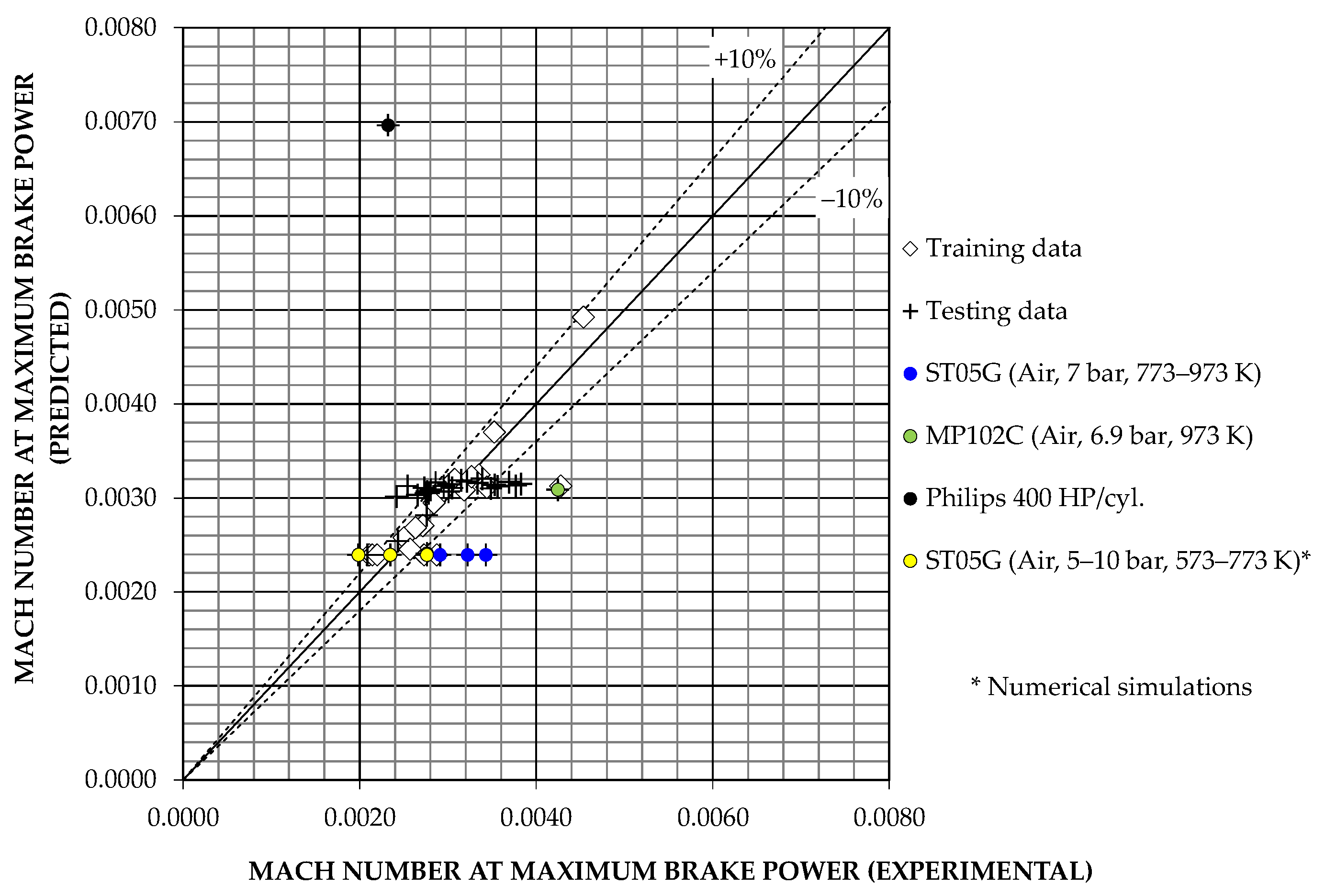
With respect to G2-model estimates of ${\zeta }_{ind,\mathrm{m}\mathrm{a}\mathrm{x}}$, both models G2-5R and G2-9ANN provide very accurate estimates for the training data, especially the G2-9ANN model. The results are also good for the testing data, with almost all relative deviations within ±10%, as shown in Figure 8 and Figure 13a, and

Table 9. Statistical indicators of the performance of the ${\zeta }_{ind,\mathrm{m}\mathrm{a}\mathrm{x}}$ models of group G2.

		RRMSE (%)	NRMSE (%)	RMBE (%)	NMBE (%)	NSE	${\mathit{R}}^2$	${\mathit{\sigma }}_{\mathit{s}\mathit{n}}$	${\mathit{E}}_{\mathit{n}}^{\mathit{\prime }}$ (%)
Training data	G2-5R	3.20	2.60	−0.17	−0.34	0.9979	0.9981	0.9905	4.49
	G2-9ANN	0.55	0.52	−0.01	−0.01	0.9990	0.9999	0.9997	0.90
All data	G2-5R	8.18	8.33	3.77	4.01	0.9700	0.9767	1.0753	17.58
	G2-5R1	6.42	6.78	3.07	3.35	0.9804	0.9848	1.0636	14.25
	G2-9ANN	6.86	7.04	3.00	3.21	0.9679	0.9762	1.0280	15.93
	G2-9ANN 1	4.81	5.25	2.32	2.56	0.9825	0.9875	1.0239	11.57

¹ Excluding the operating point No. 33 of Table A4.

.

Moreover, both models show the aforementioned anomaly of operating point No. 33 in Table A4. It is interpreted that the quality of these models is mainly due to the inclusion of the dimensionless quasi-static work per cycle ${\zeta }_0$ among the input variables, since the ratio ${\zeta }_{ind,\mathrm{m}\mathrm{a}\mathrm{x}}/{\zeta }_0$ is bounded, as indicated by Equation (4). Accuracy is also enhanced by the inclusion of additional variables, reflecting the influence of dead volume and regenerator geometry.

Regarding G2-model estimates of $N_{MA,\mathrm{m}\mathrm{a}\mathrm{x}}$, Figure 9 shows that the predictions of the G2-6R model have a good degree of accuracy, with practically all relative errors within ±10%, again excluding point No. 33 in Table A4.

In contrast, Figure 13b shows that the predictions of the G2-10ANN model with two neurons in the hidden layer, although acceptable for the training data, show high relative deviations, not only as expected for the operating point No. 33 of Table A4, but also for the operating point No. 54. The statistical indicators listed in

Table 10. Statistical indicators of the performance of the $N_{MA,\mathrm{m}\mathrm{a}\mathrm{x}}$ models of group G2.

		RRMSE (%)	NRMSE (%)	RMBE (%)	NMBE (%)	NSE	${\mathit{R}}^2$	${\mathit{\sigma }}_{\mathit{s}\mathit{n}}$	${\mathit{E}}_{\mathit{n}}^{\mathit{\prime }}$ (%)
Training data	G2-6R	6.35	7.30	0.43	0.02	0.8932	0.8934	0.9320	32.68
	G2-10ANN	7.34	6.64	−0.54	−0.88	0.9116	0.9131	0.9591	29.48
All data	G2-6R	9.94	0.23	−4.93	−0.10	0.6589	0.7325	1.1284	58.46
	G2-6R 1	8.74	0.16	−4.29	−0.07	0.8209	0.8649	1.1407	42.37
	G2-10ANN	13.54	12.53	2.14	0.81	0.6103	0.6160	0.8490	62.30
	G2-10ANN 1	12.91	11.07	2.87	1.80	0.6801	0.6917	0.8878	55.81
	G2-10ANN 2	12.28	10.60	3.62	2.35	0.7019	0.7172	0.8229	53.23

¹ Excluding the operating point No. 33 of Table A4. ² Excluding the operating points No. 33 and No. 54 of Table A4.

show that the G2-6R model is somewhat better than the G2-10ANN model, especially for operating point No. 54. However, deviations for operation point No. 54 can be considered less relevant, as this prototype was never built [46], and the corresponding values of the input variables ${\zeta }_0$, ${r_{hR}^{2}L}_R/V_0$, $\sum {\mu }_{dx}$ and $N_p$ are outside the range of the training data variables and at the extremes of the test data range. In summary, it seems that a neural network with a more complex structure would be necessary to outperform the accuracy of the $N_{MA,\mathrm{m}\mathrm{a}\mathrm{x}}$ predictions obtained by the regression-based model.

With respect to G2-model estimates of ${\zeta }_{B,\mathrm{m}\mathrm{a}\mathrm{x}}$, Figure 10 and

Table 11. Statistical indicators of the performance of the ${\zeta }_{B,\mathrm{m}\mathrm{a}\mathrm{x}}$ models of group G2.

		RRMSE (%)	NRMSE (%)	RMBE (%)	NMBE (%)	NSE	${\mathit{R}}^2$	${\mathit{\sigma }}_{\mathit{s}\mathit{n}}$	${\mathit{E}}_{\mathit{n}}^{\mathit{\prime }}$ (%)
Training data	G2-7R	6.39	5.23	−0.44	−1.02	0.9930	0.9935	0.9812	8.21
	G2-11ANN	3.68	4.73	−0.14	−0.43	0.9943	0.9944	0.9869	7.54
All data1	G2-7R	11.74	14.26	−1.04	−0.72	0.9183	0.9241	1.0360	28.55
	G2-7R 1	11.24	13.87	−1.58	−1.27	0.9238	0.9284	1.0270	27.50
	G2-7R 2	11.11	13.72	−1.29	−0.85	0.9256	0.9311	1.0371	27.22
	G2-11ANN	18.14	15.98	−1.13	0.15	0.8655	0.8911	1.1038	36.67
	G2-11ANN 1	17.94	15.68	−1.65	−0.37	0.8730	0.8969	1.0993	35.63
	G2-11ANN 2	17.28	13.98	−2.43	−1.44	0.9009	0.9139	1.0655	31.32

¹ Excluding the operating point No. 33 of Table A4. ² Excluding the operating points No. 33 and No. 54 of Table A4.

show that the predictions of the G2-7R model fit most of the data used for its construction, but the deviations are relatively large for several of the test data. The highest percentage deviations are for some points of the MP102C engine operating at 873 K and the ST05G engine, although it should be noted that the latter data are from simulations. The relative deviations of points No. 33 and No. 54 are again outside the limits of ±10%.

The results are similar using the G2-11ANN model, as shown in Table 11 and Figure 13c, apart from the 400 HP/cylinder prototype, for which this model predicts higher relative deviation. These observations show that both types of models can be acceptable for preliminary design, although their estimation capability is limited by not including input variables related to the mechanical losses of indicated power. Future improvements can be expected from the inclusion of input variables representative of mechanical efficiency, the availability of more operational data, and the use of neural networks with more complex structure.

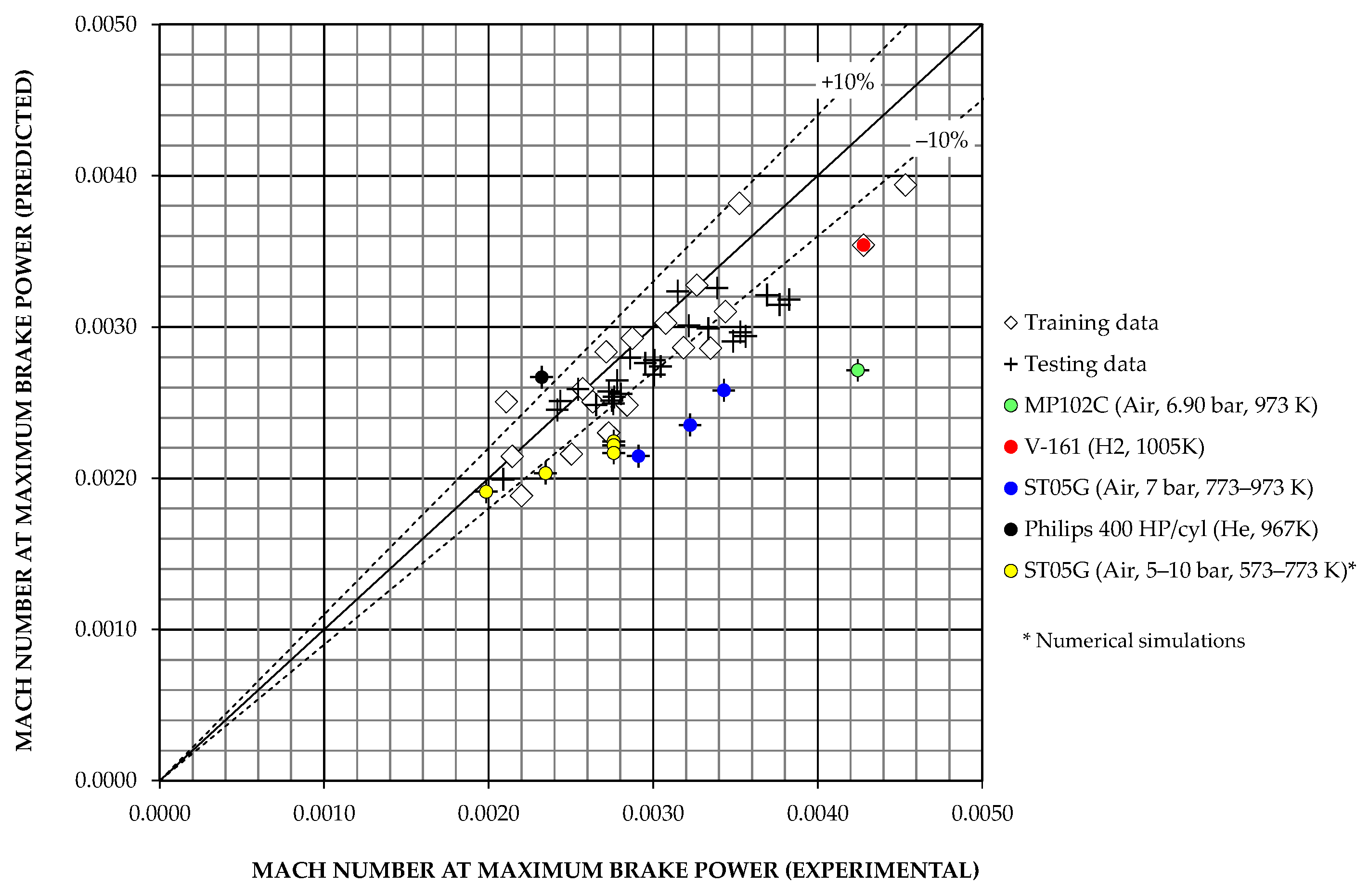
In the case of the G2-model estimates of $N_{MA,\mathrm{m}\mathrm{a}\mathrm{x}}^{*}$, Figure 11 shows that the predictions of the G2-8R model are accurate for most of the data used to construct the correlation, as they are virtually all included within the ±10% deviation limits. For the test data, in general, the model predictions are biased below the target data. Apart from operating point No. 33 in Table A4, the largest percentage deviations, in the order of −25%, correspond to points in the ST05G engine series.

Furthermore, Figure 13d shows that the predictions of the G2-12ANN model with two neurons in the hidden layer are acceptable for the training data, but show high relative deviations for operating point No. 54 of Table A4 and, to a lesser extent, for several points in the ST05G engine series. In order to improve the results, the G2-12ANN model was modified by arranging one neuron in the hidden layer, with the statistical effects shown in

Table 12. Statistical indicators of the performance of the $N_{MA,\mathrm{m}\mathrm{a}\mathrm{x}}^{*}$ models of group G2.

		RRMSE (%)	NRMSE (%)	RMBE (%)	NMBE (%)	NSE	${\mathit{R}}^2$	${\mathit{\sigma }}_{\mathit{s}\mathit{n}}$	${\mathit{E}}_{\mathit{n}}^{\mathit{\prime }}$ (%)
Training data	G2-8R	10.93	11.56	−5.15	−5.92	0.7164	0.7925	0.1804	84.34
	G2-12ANN 1	8.68	10.85	−0.76	−1.16	0.7500	0.7767	1.0358	49.71
	G2-12ANN 2	10.07	11.69	−0.96	−1.87	0.7097	0.7259	0.9455	53.18
All data1	G2-8R	13.32	14.82	−8.71	−9.61	0.3629	0.5947	0.8238	63.88
	G2-8R 3	12.50	13.30	−8.19	−8.89	0.4527	0.6733	0.8648	57.33
	G2-8R 4	12.45	13.28	−8.64	−9.25	0.4437	0.6824	0.8774	56.59
	G2-12ANN 1	43.37	35.72	3.33	1.33	−2.7100	0.0541	1.8922	192.36
	G2-12ANN 1,3	19.47	19.13	−1.66	−2.36	−0.1500	0.3347	1.2670	106.74
	G2-12ANN 2	30.13	25.36	2.49	0.22	−0.8675	0.0835	1.2640	136.65
	G2-12ANN 2,3	30.18	25.24	3.05	0.96	−0.9793	0.0888	1.3301	140.59
	G2-12ANN 2,4	12.63	13.24	−0.73	−2.03	0.4454	0.4812	0.8447	73.59

¹ Using 2 neurons in the hidden layer. ² Using 1 neuron in the hidden layer. ³ Excluding the operating point No. 33 of Table A4. ⁴ Excluding the operating points No. 33 and No. 54 of Table A4.

, depending on whether or not operating points No. 33 and 54 are included. Figure 15 shows the results with the modified model.

As in the case of the ${\zeta }_{B,\mathrm{m}\mathrm{a}\mathrm{x}}$ models in group G2, future improvements of the G2-8R and G2-12ANN models could be based on more complexly structured neural networks and on seeking reliable training and test data, whose ranges of variation are similar once expressed in dimensionless variables.

All in all, the most pressing need for future work is to increase the amount of available experimental data. Uncertainty of existing data can be addressed by different techniques already successfully used in artificial intelligence and deep learning, such as clustering, backpropagation, Benders decomposition or option value [54,55,56]. Furthermore, variants of the procedure used in this article for eight-input models could be interesting for other energy conversion systems, since Equation (2) is applicable to other thermodynamic cycles [27].

5. Conclusions

Regression-based models and simple ANNs have been developed and compared to estimate the peak power values for feasibility studies and the preliminary design of Stirling engines. The main findings are summarised below:

• Models using three dimensionless input variables fit the 89 operating data points from 34 engines, with relative errors of about ±25%. The classical correlations are not adequate for a significant number of data, and do not provide criteria for estimating the speed corresponding to the peak power points;
• Estimates of the dimensionless maximum indicated power from models using eight dimensionless input variables match practically all the operating data, with relative errors within ±10%, for both regression-based and ANN-based models. The regression-based model estimates are also quite accurate for the corresponding dimensionless engine speeds, while the ANN-based model predicts acceptable relative errors for the training data, but larger deviations for some test data;
• Estimates of dimensionless maximum brake power from models using eight dimensionless input variables are also acceptable for data used in building regression models or training ANN models, but the deviations are somewhat less accurate for test data. The predictions of the corresponding engine speeds show similar relative deviations for both regression-based and ANN models. Such deviations are related to the lack of input variables involved in the mechanical efficiency, whose inclusion is recommended for future works.