
An Investigation on the Vortex Effect of a CALM Buoy under Water Waves Using Computational Fluid Dynamics (CFD)


Abstract
1. Introduction
2. Theoretical Model
2.1. Motion Forces, Drag and Damping Formulation
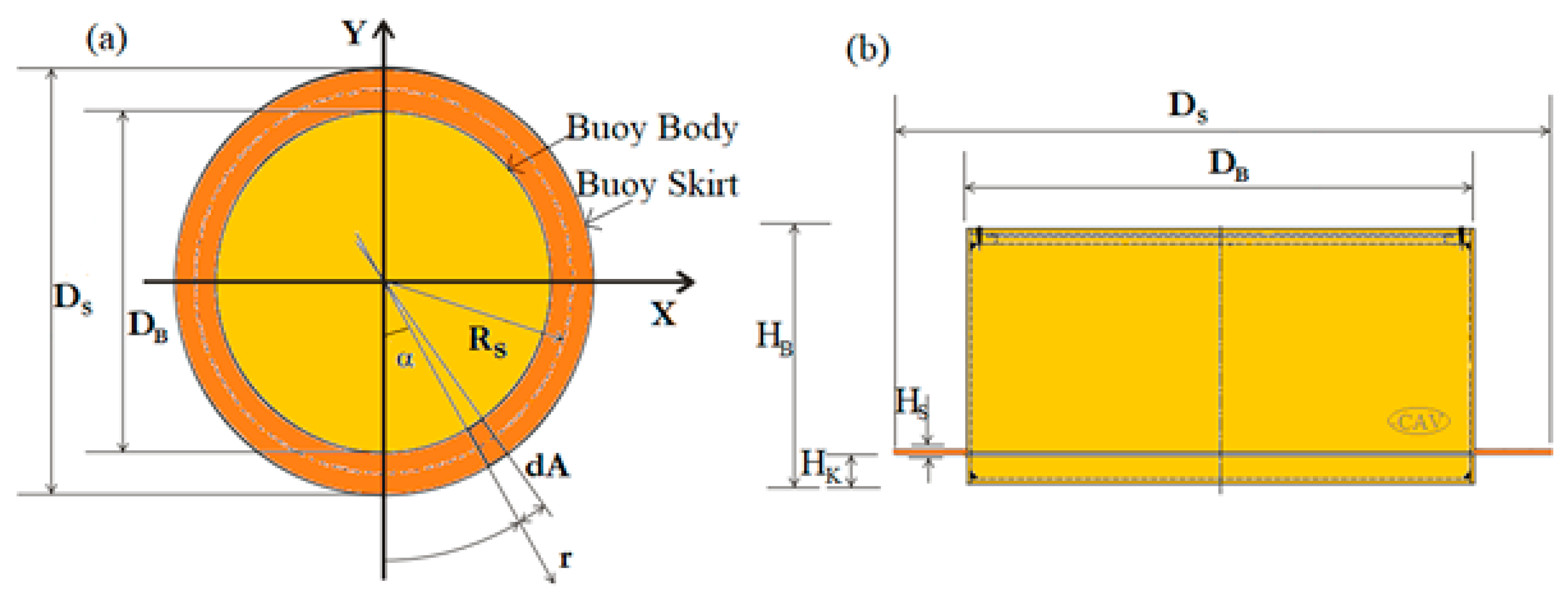
2.1.1. Buoy Model Assumptions
- The body of the CALM buoy model is cylindrically shaped;
- The buoy has a circular skirt attached to it;
- The skirt is made from solid plates with thin thickness;
- The skirt is devoid of perforations, except where fairleads or mooring lines are attached;
- Viscous contributions of damping from skin friction can be neglected;
- It is assumed that the linear radiation-diffraction computations can be utilised to obtain the CALM buoy’s damping and added masses in the following: linear heave, linear surge, and linear pitch;
- It is assumed that the drag loads on the CALM buoy’s bilges are very small;
- It is assumed that the drag loads on the CALM buoy’s skirt can influence the quadratic pitch and heave damping contributions;
- The local fluid velocity around the skirt’s circumferential area utilised in computing these damping contributions. This is conducted by considering the CALM buoys’ velocity, but ignoring the flow’s disturbance due to the buoy’s presence and the wave orbital motions;
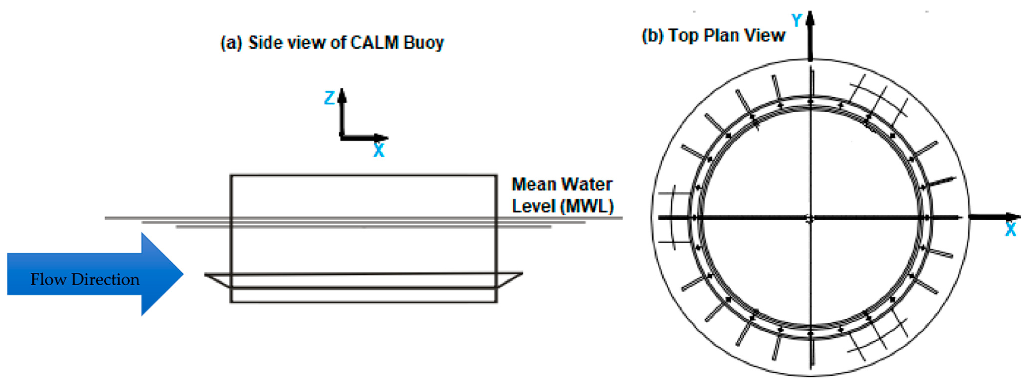
- It is assumed that the CALM buoy hull is positioned in X-Z axes, and subject to a flow direction;
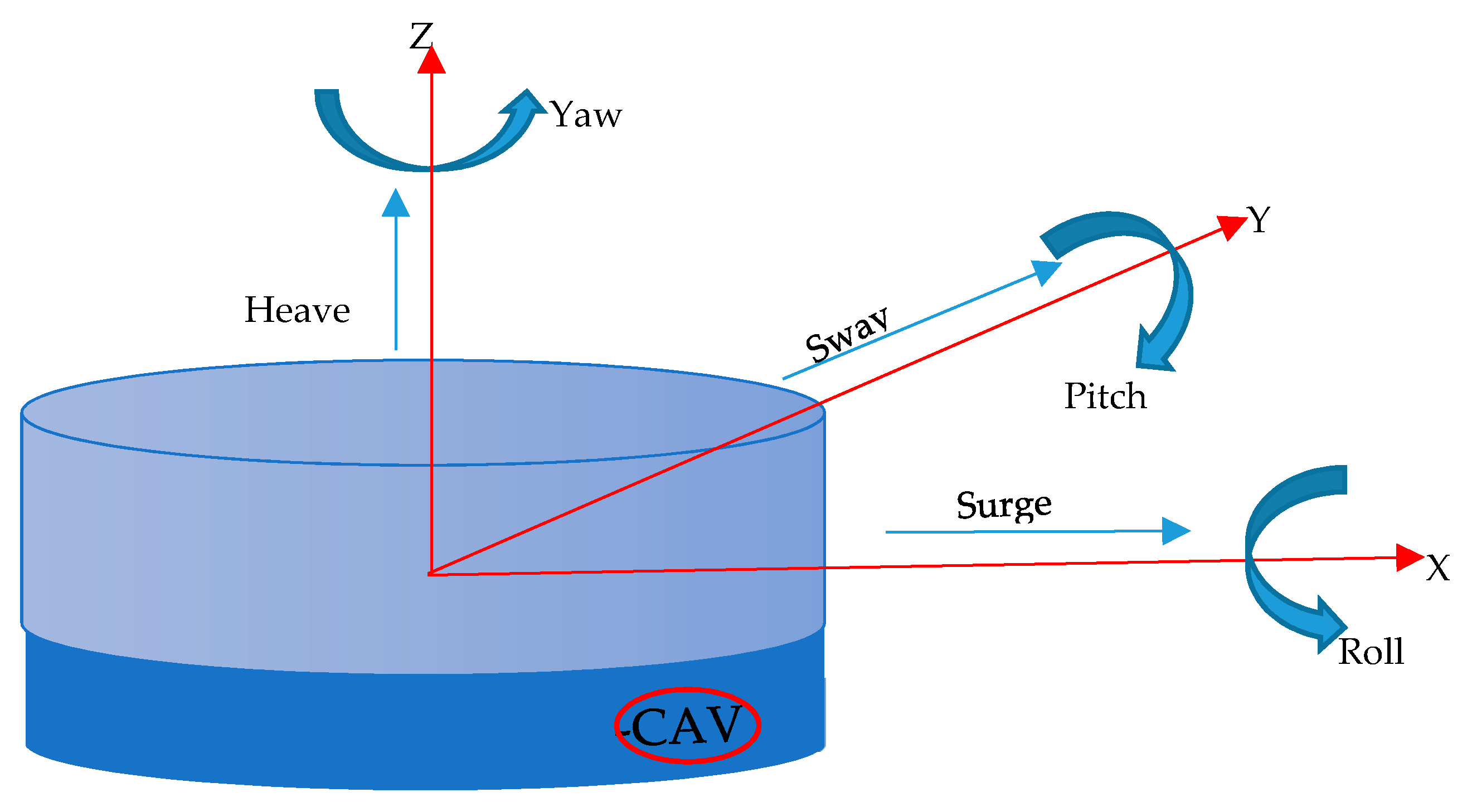
- The buoy has 6 degrees of freedom (6DoFs) as illustrated in Figure 3. The buoy is considered typically as a single system, and as a floating buoy with a rigid body.
2.1.2. Added Mass & Damping Coefficients
2.1.3. Load Computations on Buoy’s Skirt
2.1.4. Viscous Damping Load Computations
2.1.5. Damping Computations on Buoy
2.1.6. Force Computations on Buoy
2.2. FSI Formulation & Governing Equations
2.2.1. Newton’s 2nd Law of Motion
2.2.2. Navier-Stokes Equations
2.2.3. Continuity Equations
2.2.4. Morison’s Equations
3. Numerical Model
3.1. Model Description
3.2. CFD Model
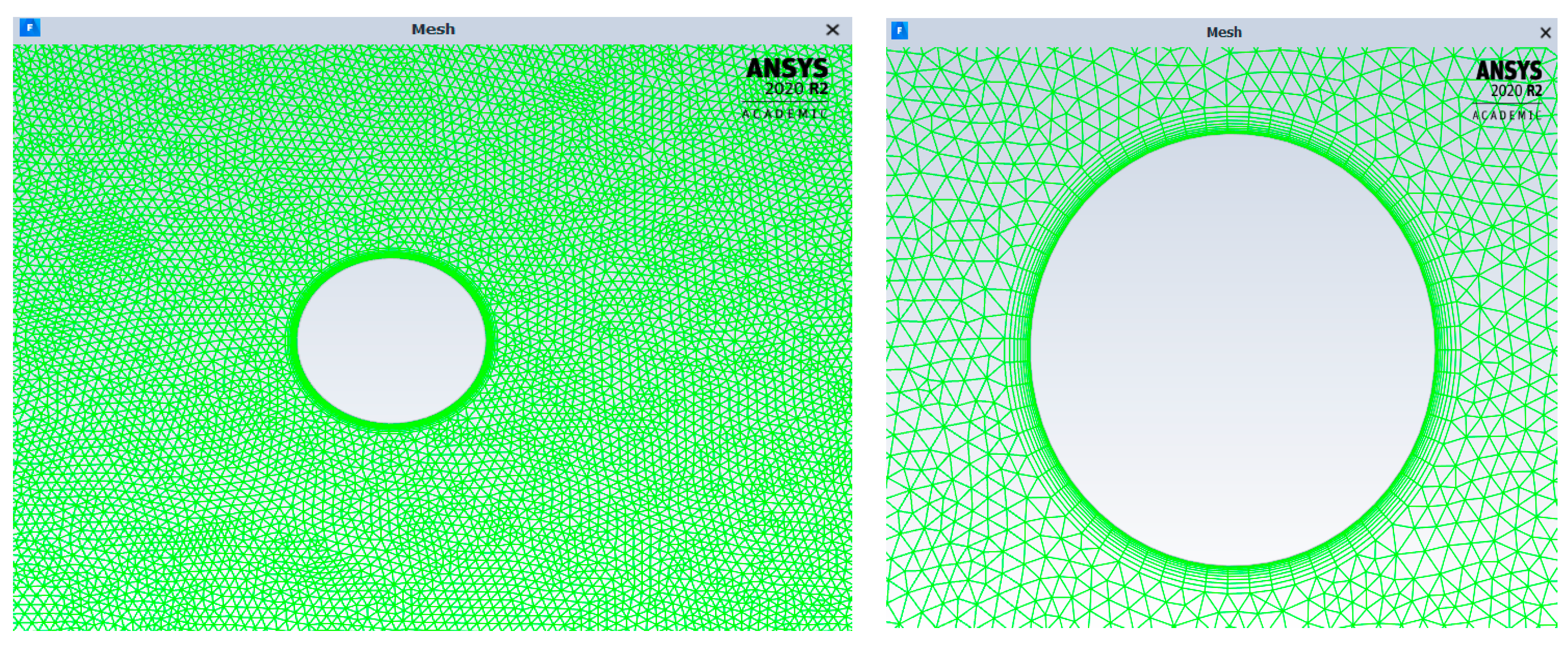
3.3. Mesh Details
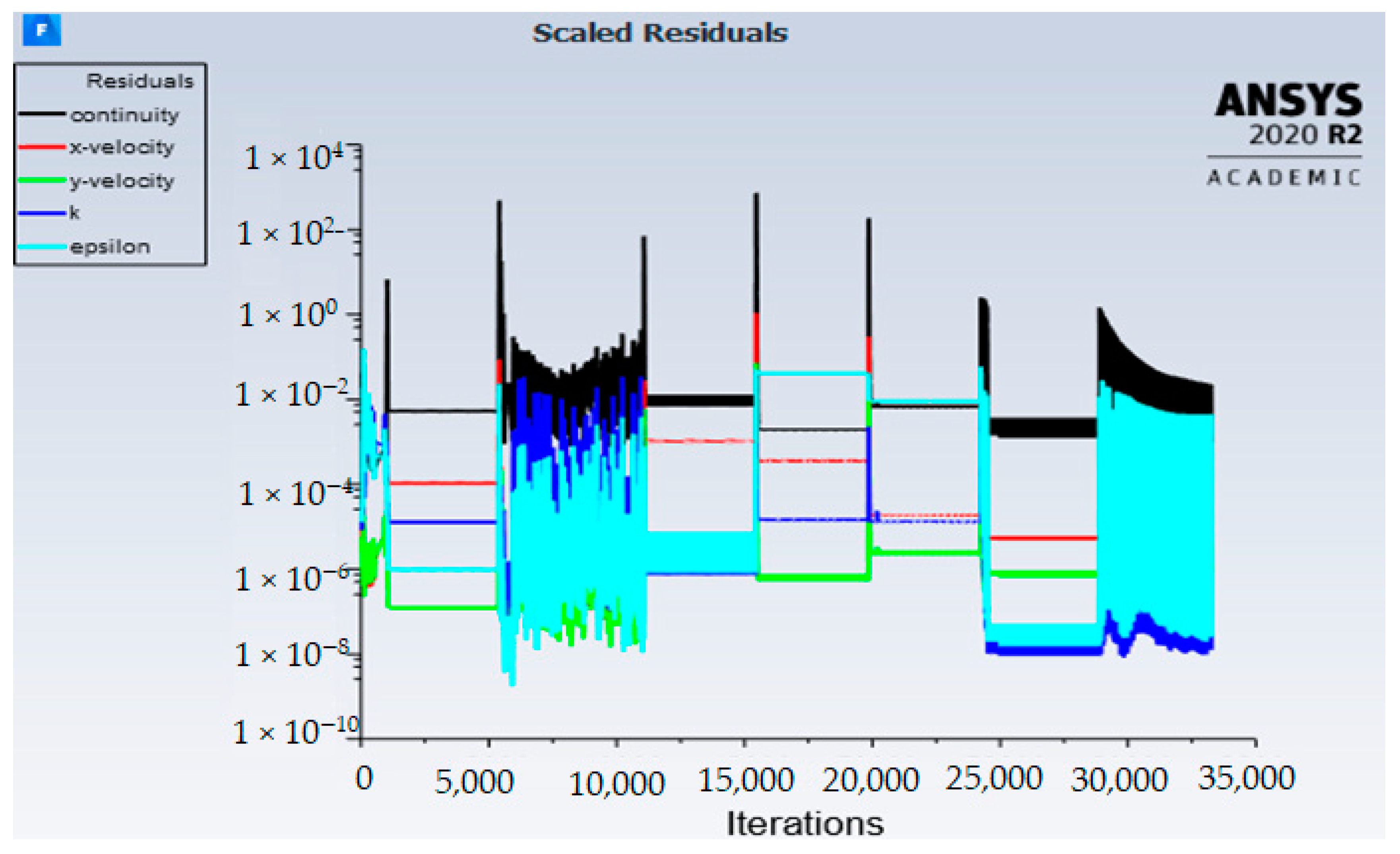
3.4. Solution Method
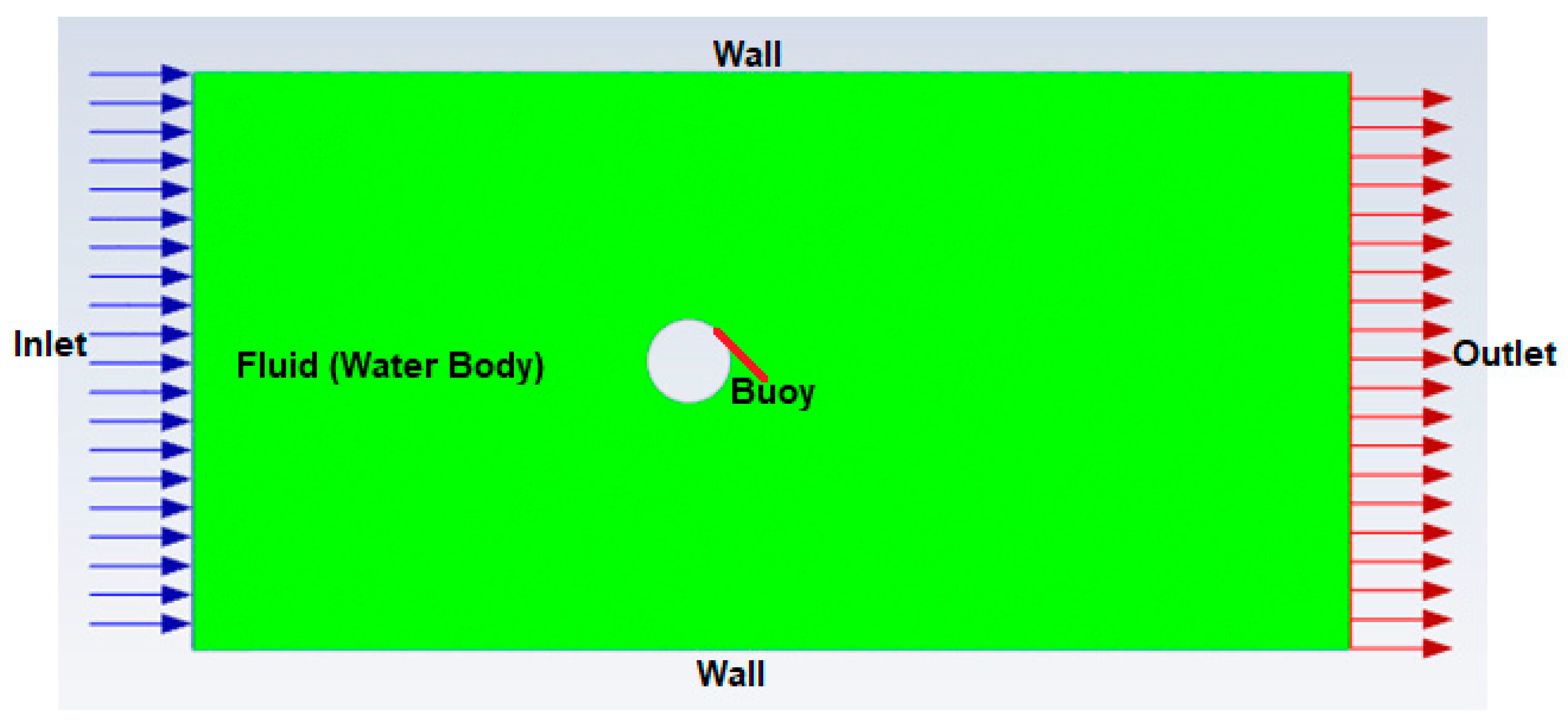
3.5. Boundary Conditions
3.6. Materials & Fluid Structure Interaction
4. Result and Discussion
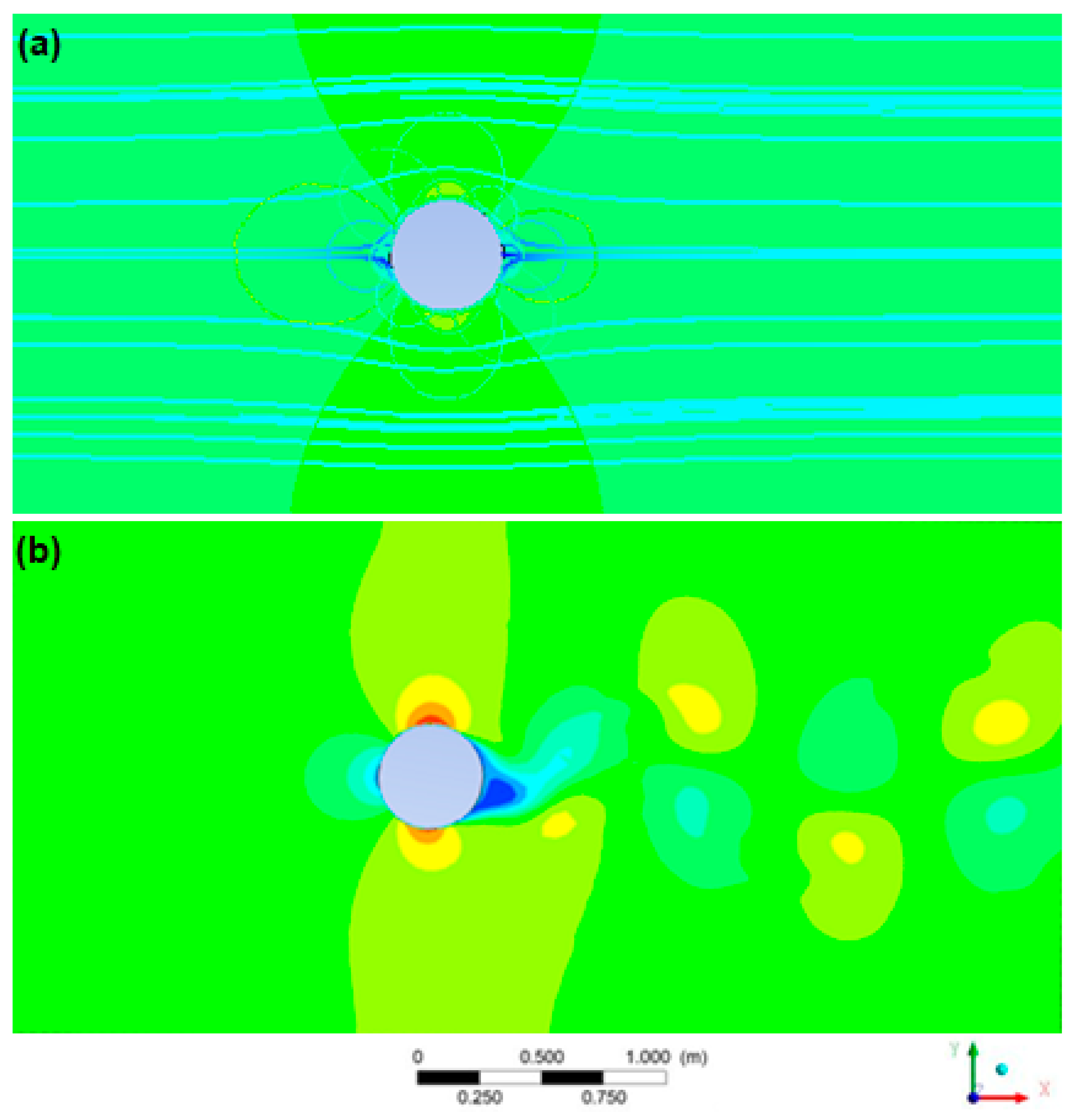
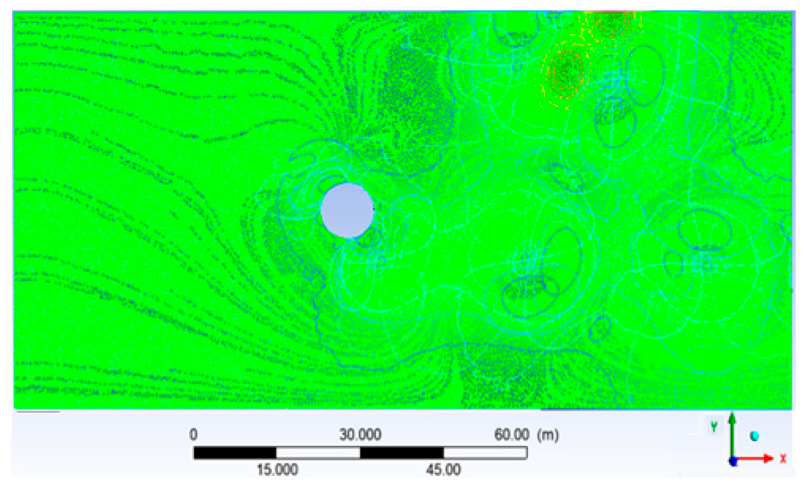
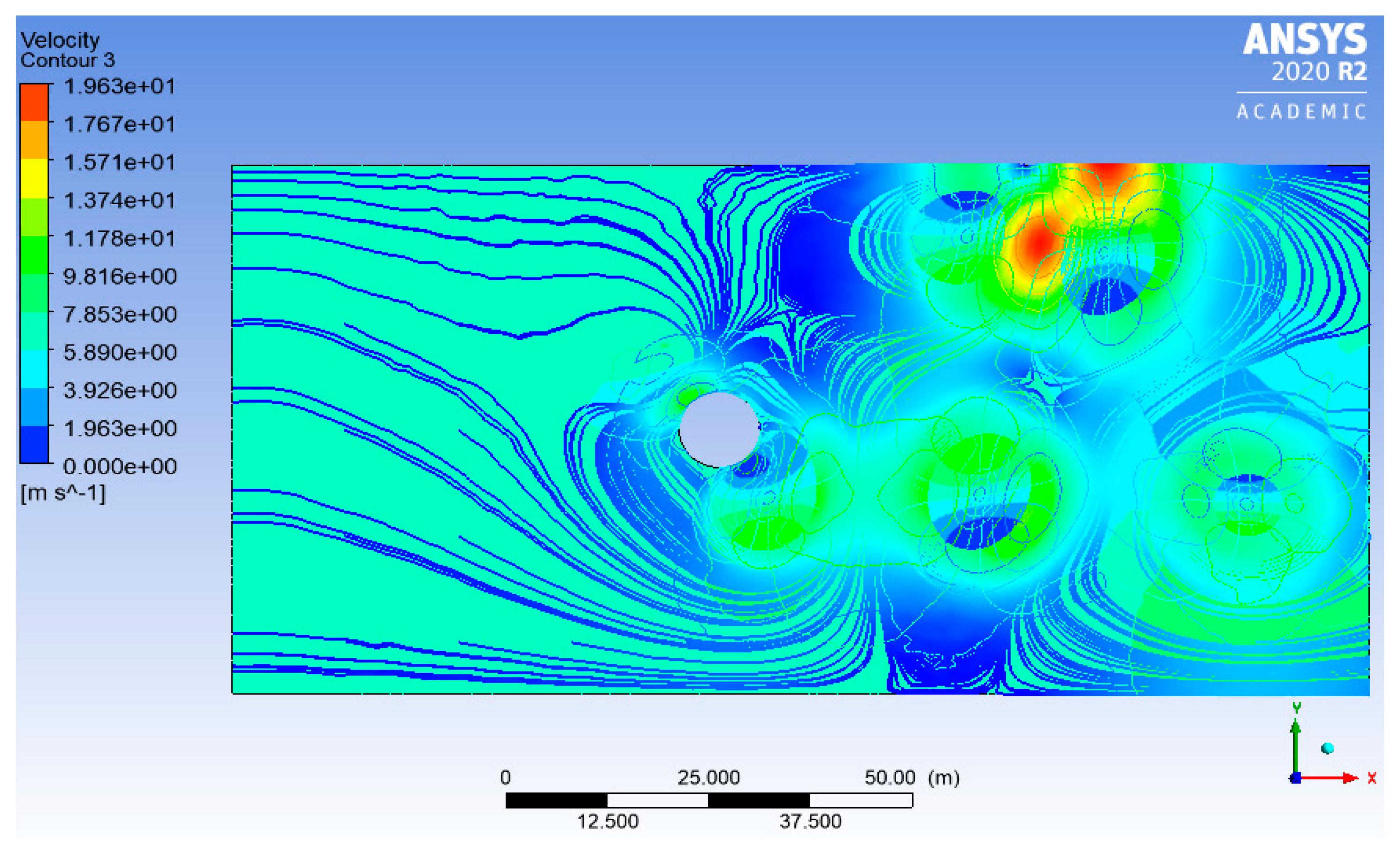
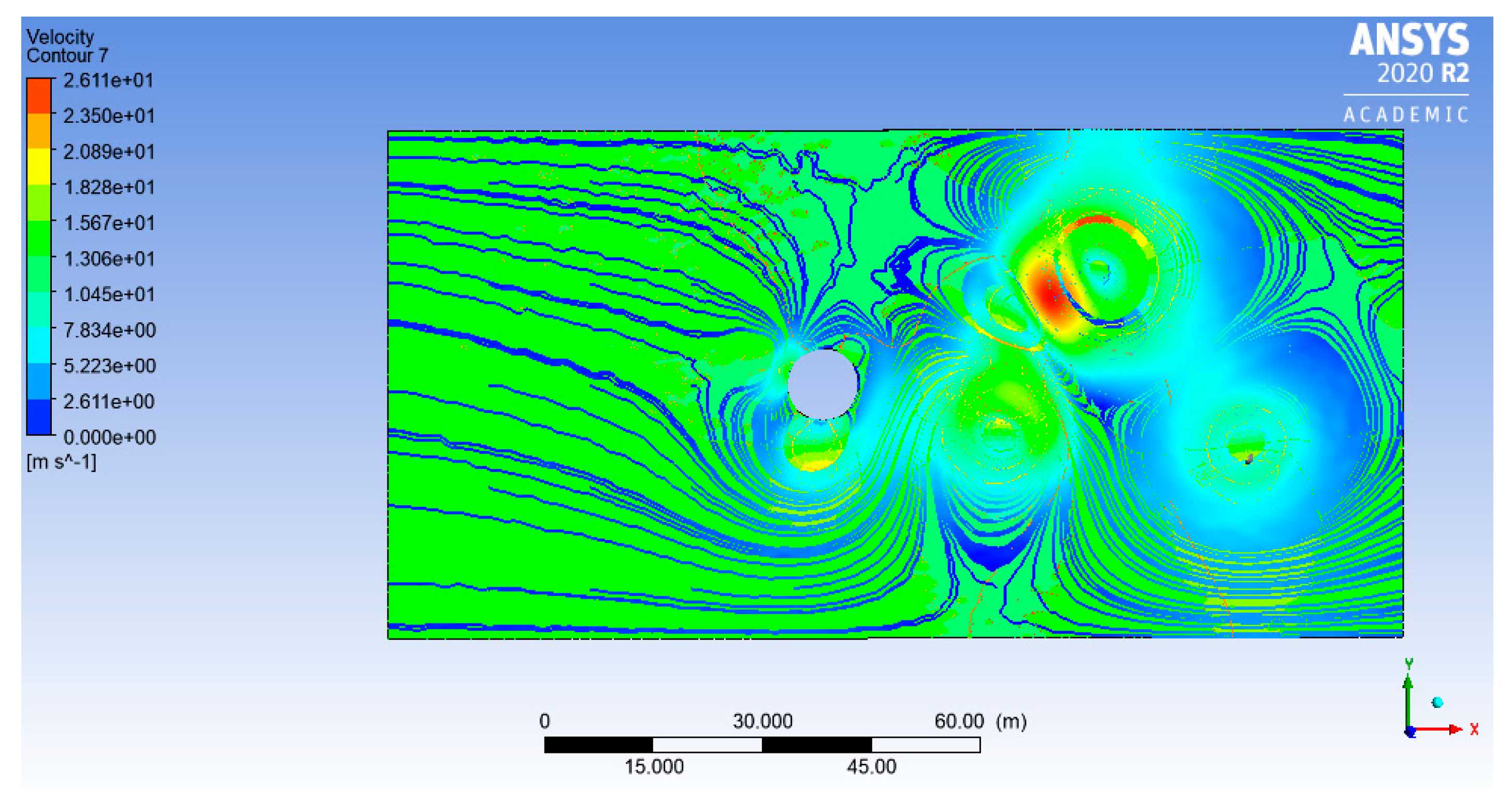
4.1. Results of Flow Vorticity around Buoy
4.2. Results of Vortex Effect from the Flow Regimes
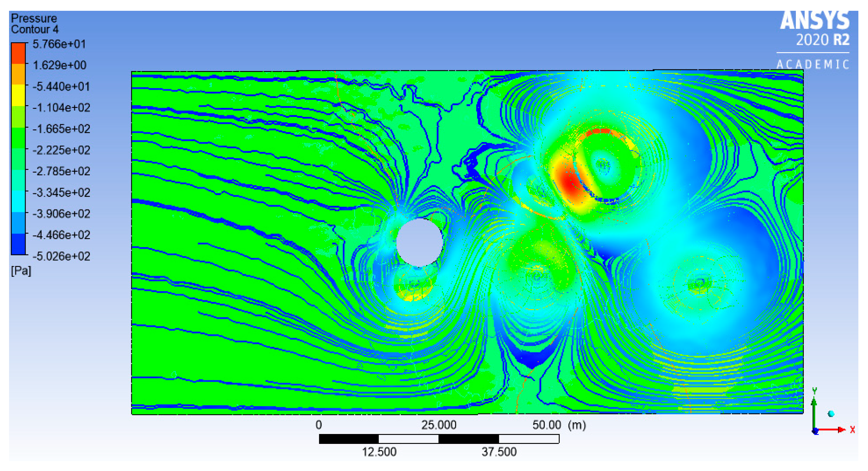
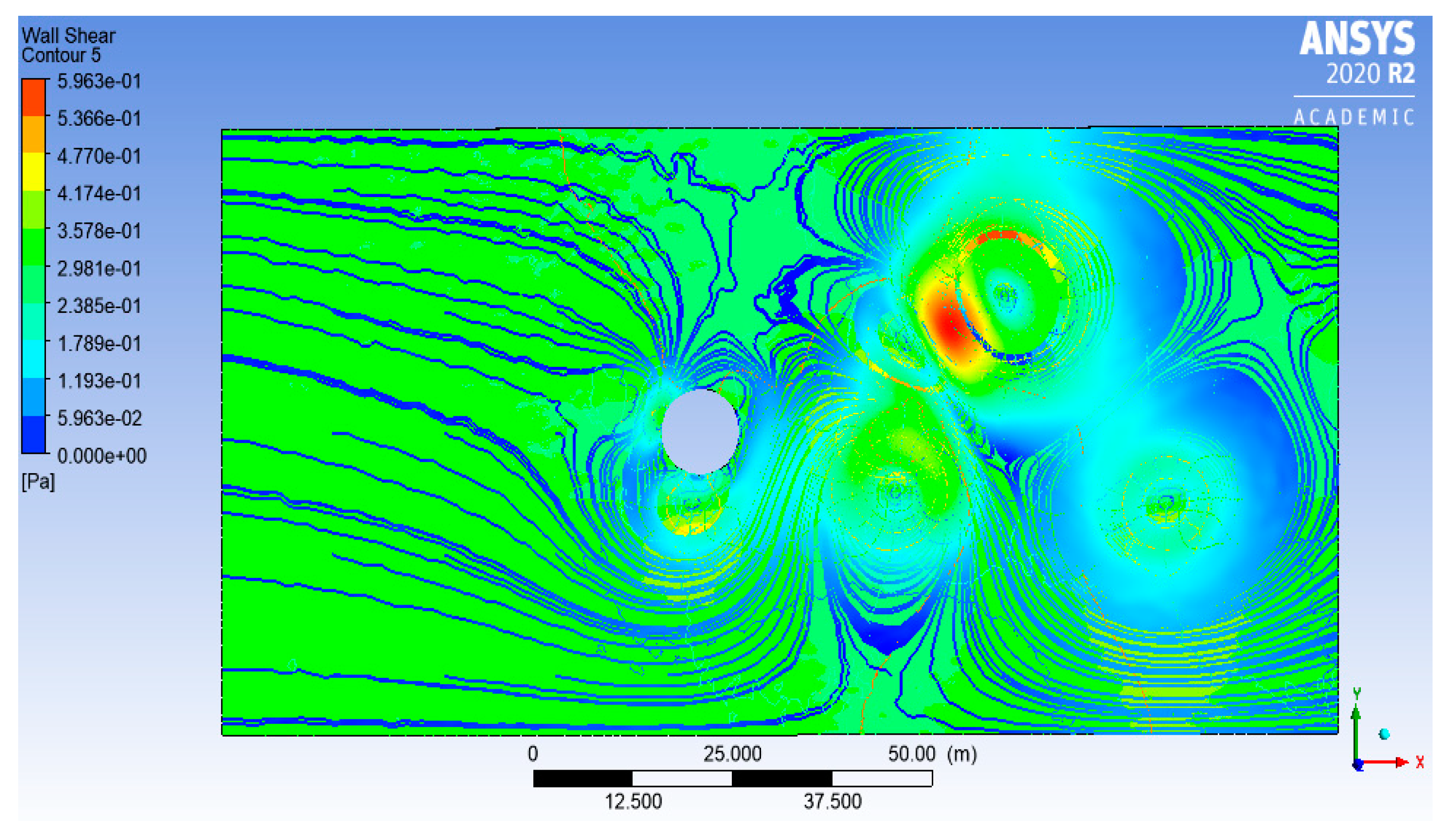
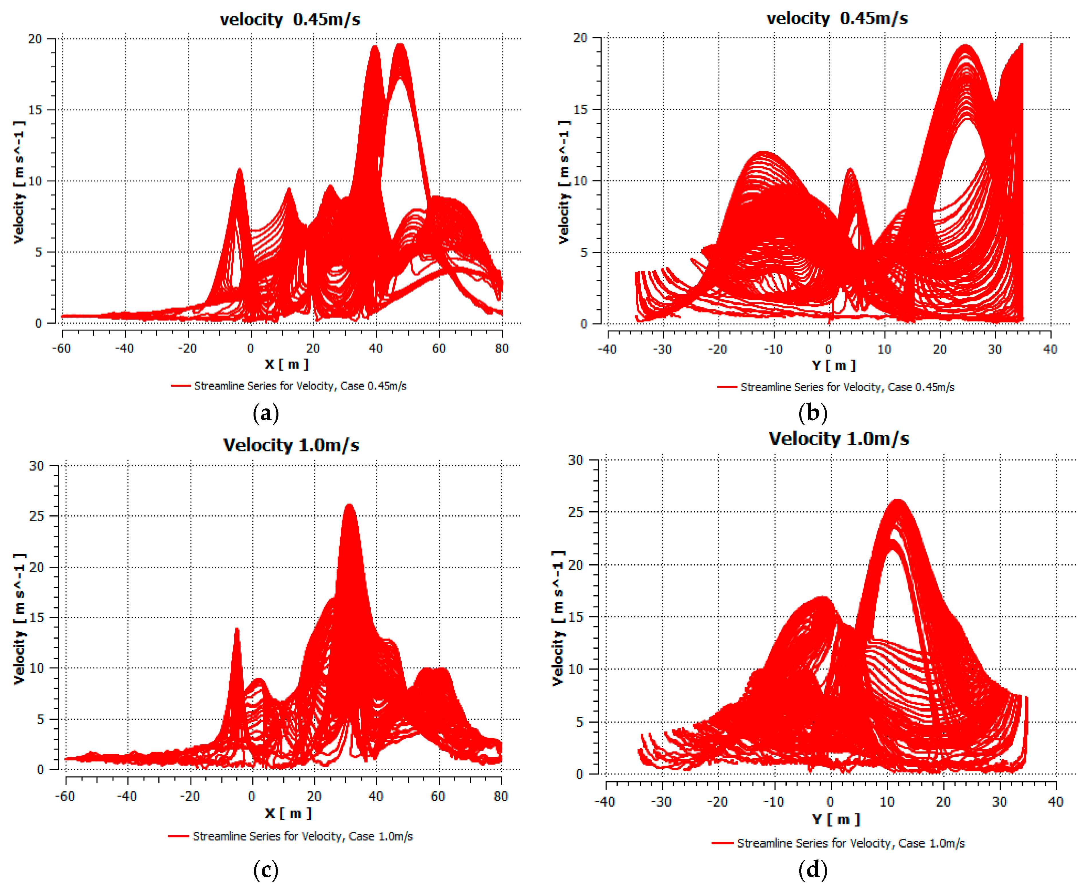
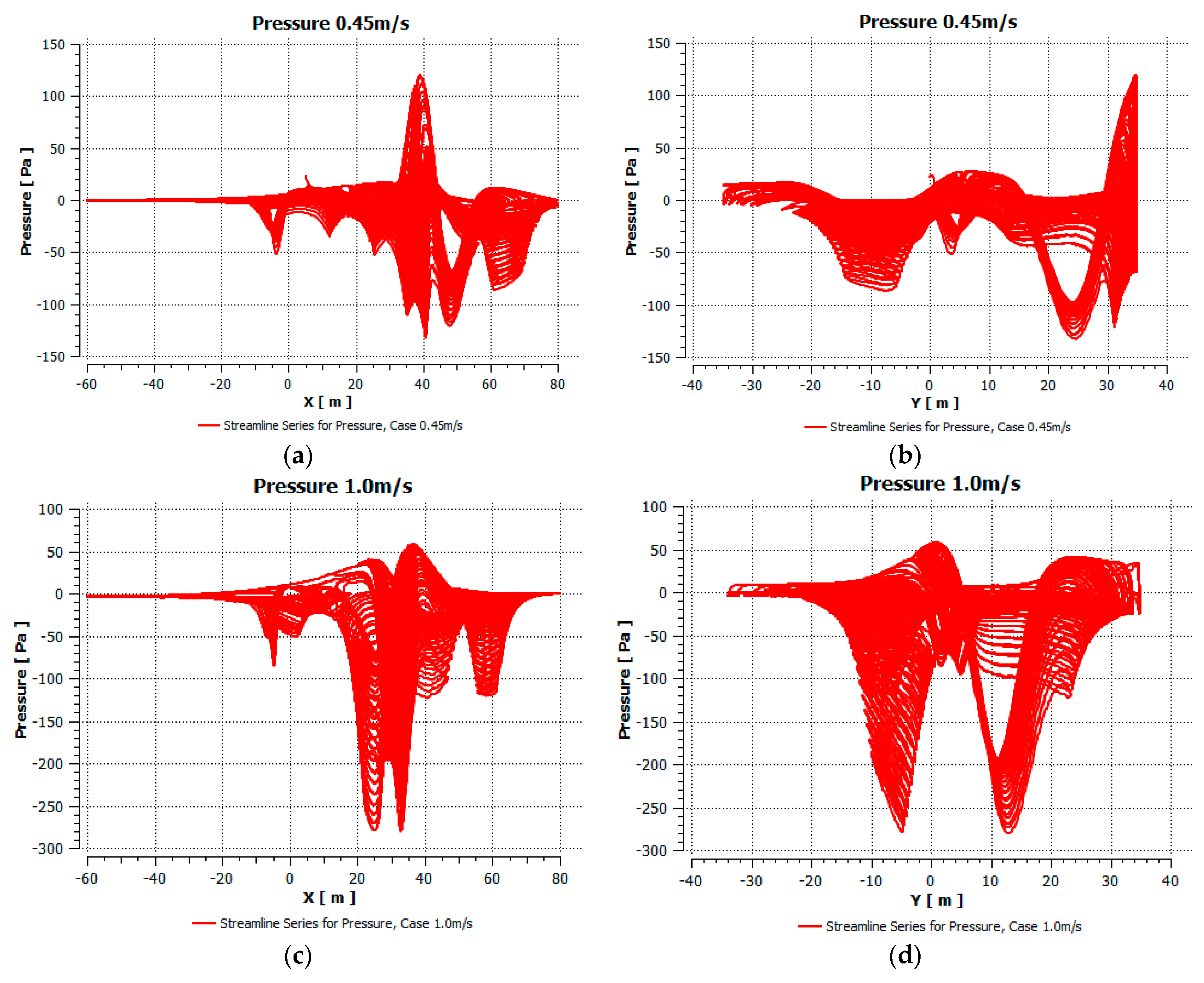
4.3. Results of Pressure, Velocity and Wall Shear Profiles on the Buoy
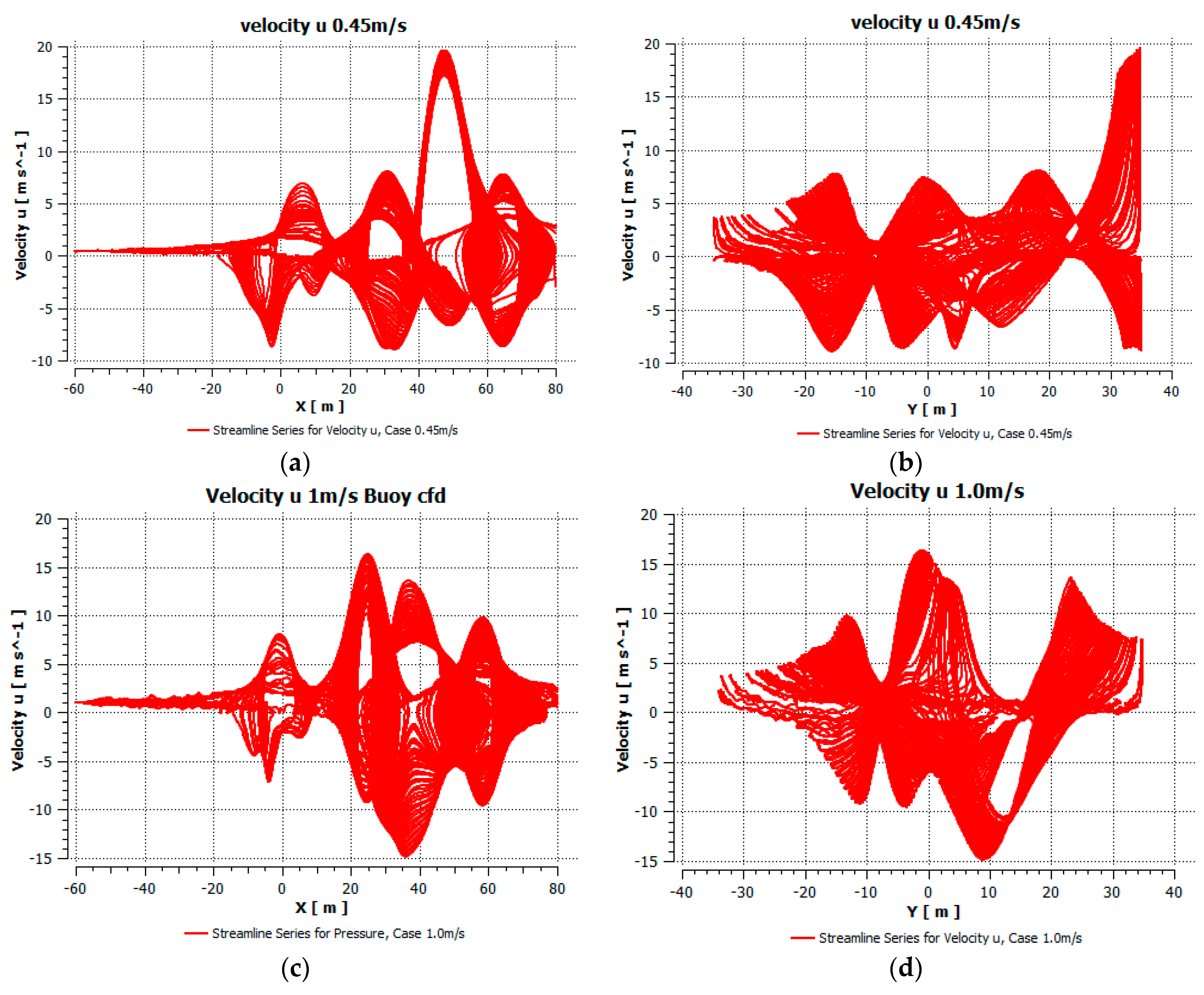
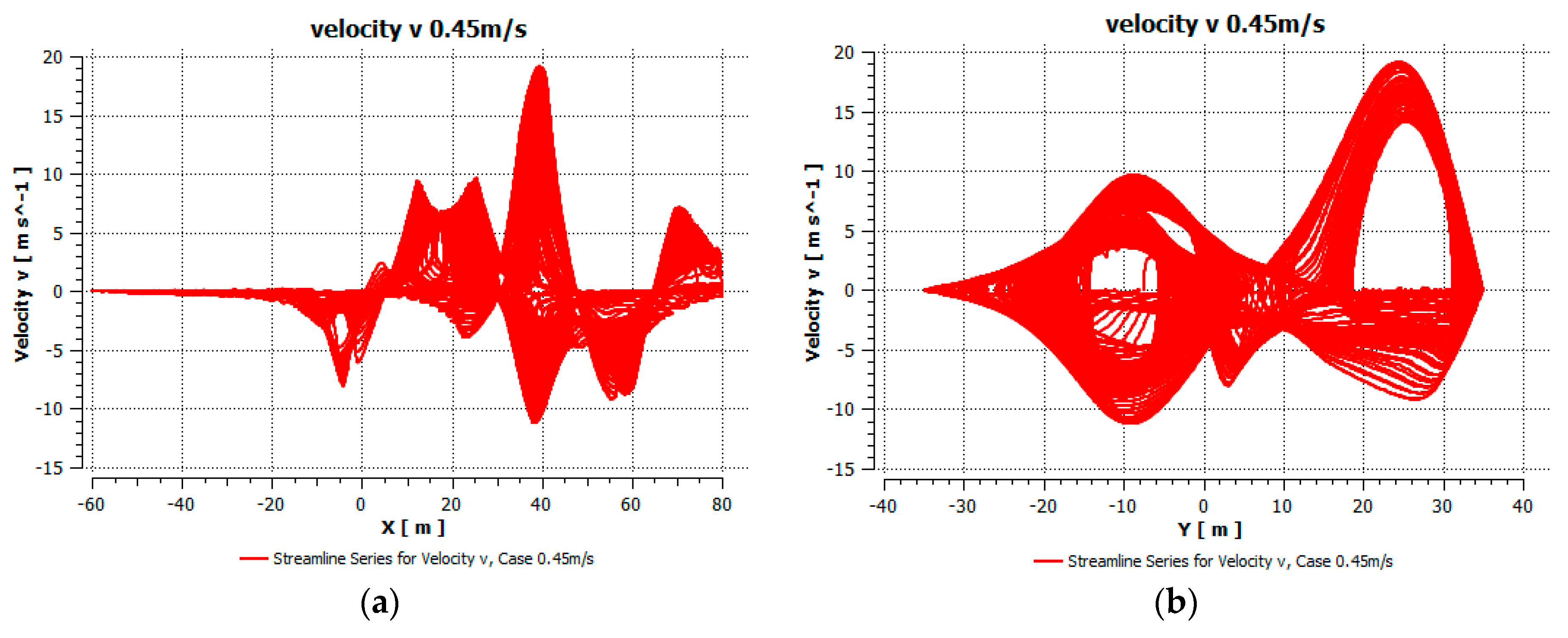
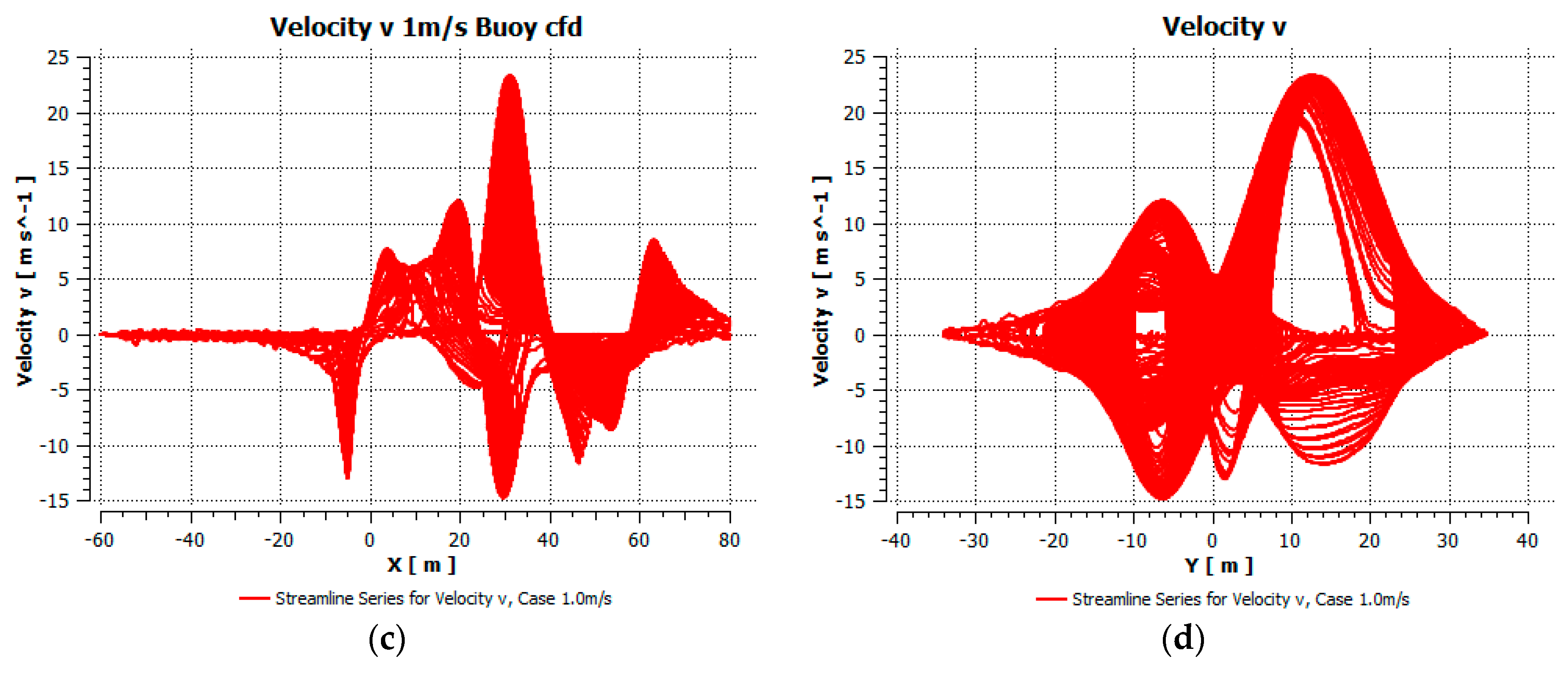
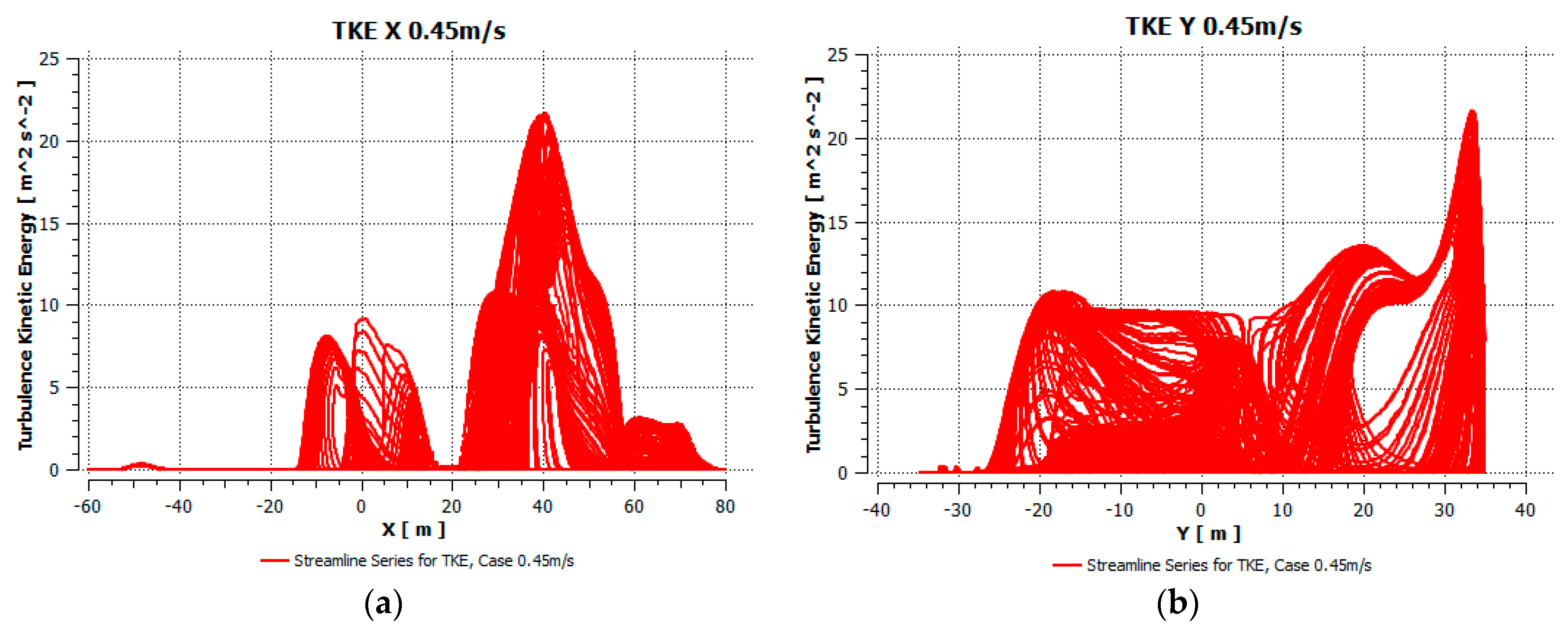
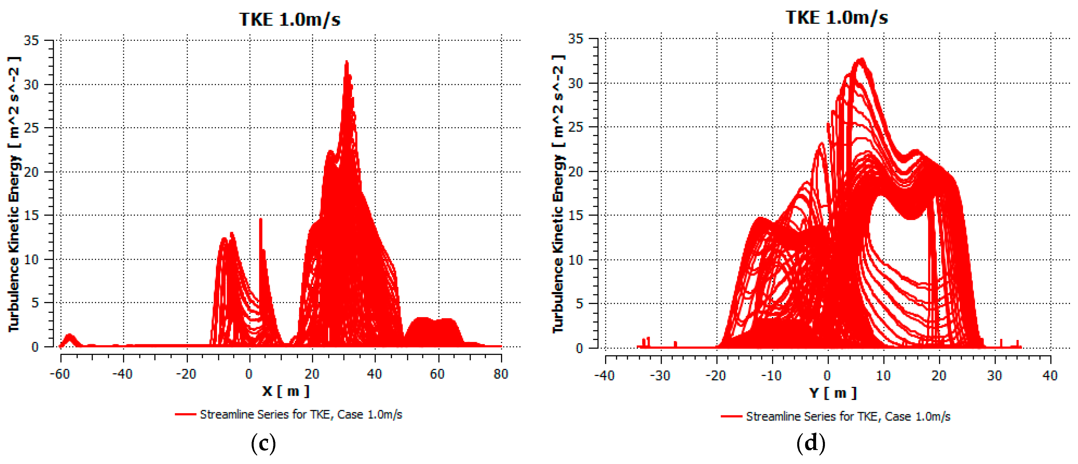
4.4. Results of Turbulence Streamlines
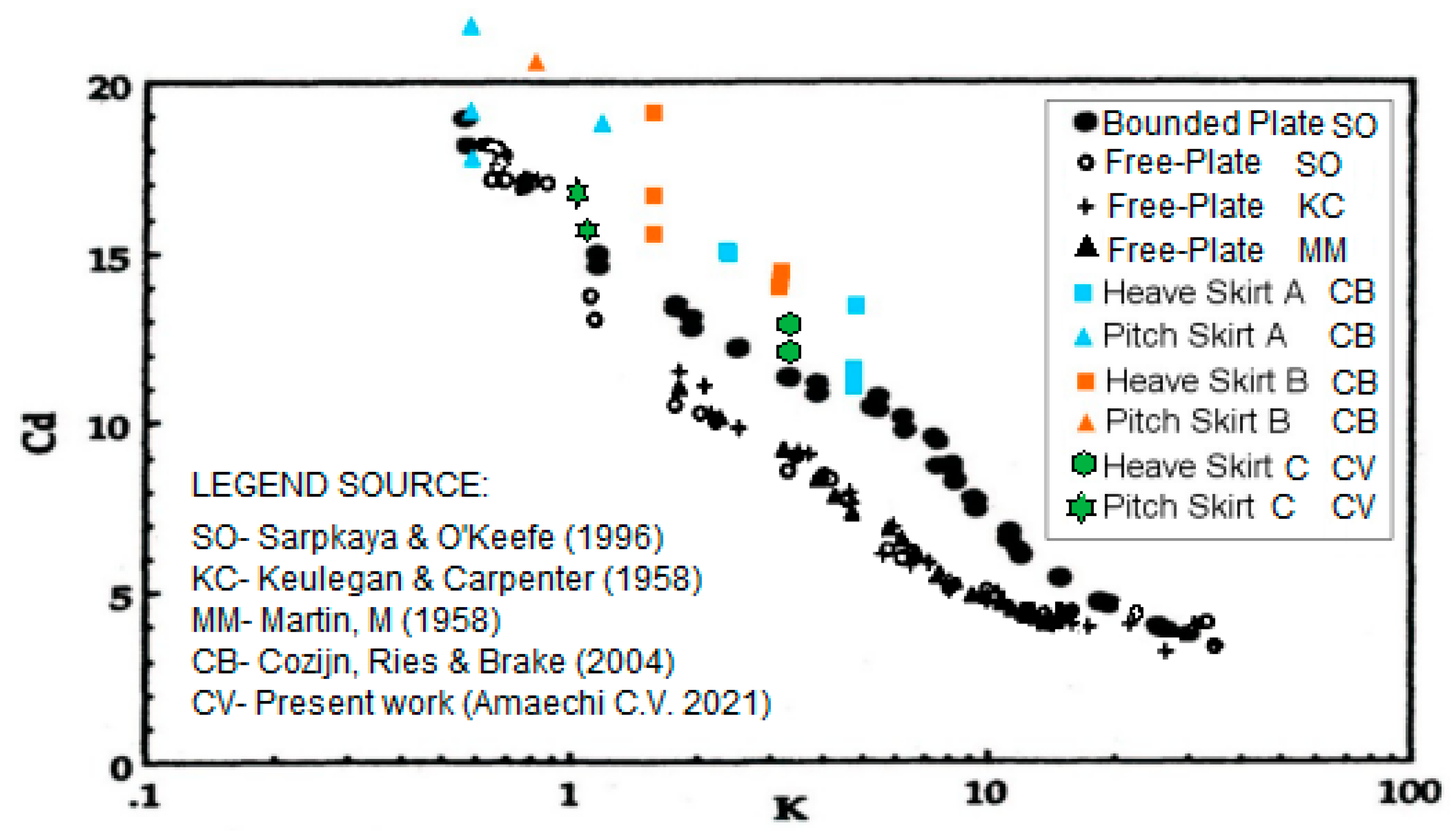
4.5. Results of Viscous Damping
5. Conclusions
Author Contributions
Funding
Institutional Review Board Statement
Informed Consent Statement
Data Availability Statement
Acknowledgments
Conflicts of Interest
Abbreviations
| 2D | Two Dimensional |
| 3D | Three Dimensional |
| 6DoF | Six Degrees of Freedom |
| AS | Area of the skirt |
| ABS | American Bureau of Shipping |
| API | American Petroleum Institute |
| ASME | American Society of Mechanical Engineers |
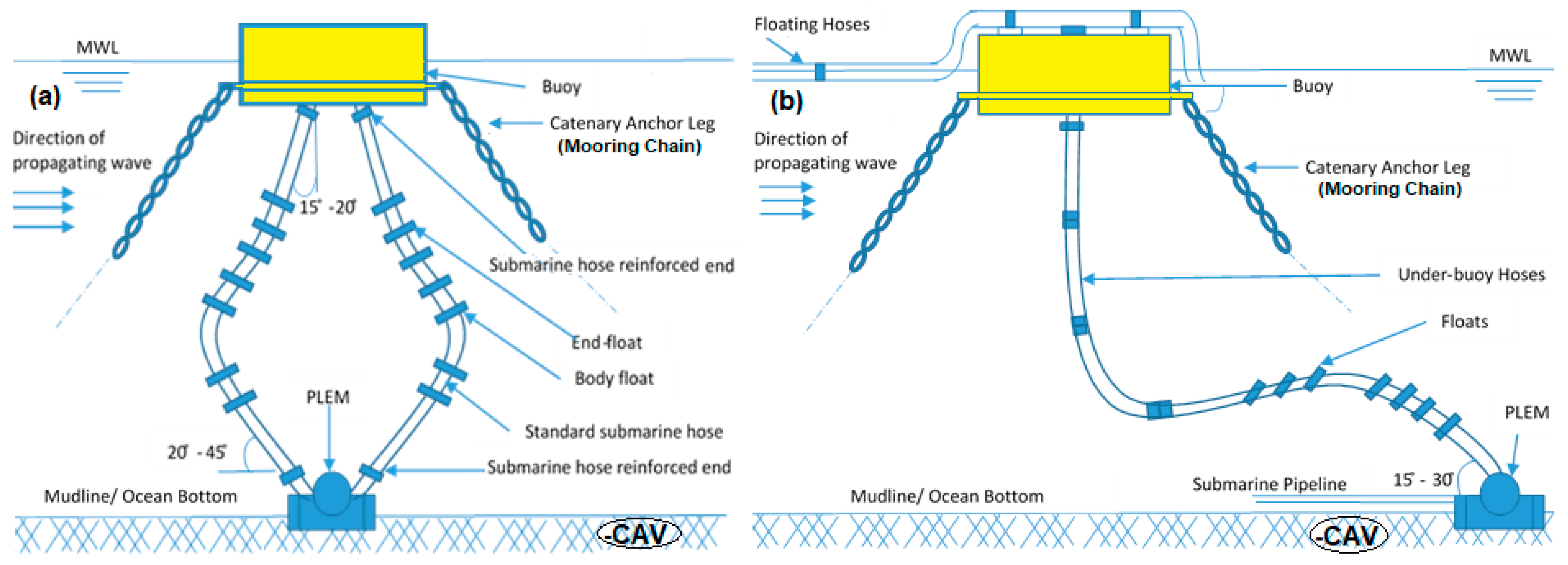
| CALM | Catenary Anchor Leg Mooring |
| CB | Cylindrical Buoy |
| CD | Dimensionless Drag Coefficient |
| CFD | Computational Fluid Dynamics |
| CMS | Conventional Mooring Systems |
| Cv | Viscous damping |
| DB | Diameter of the buoy |
| DS | Diameter of the skirt |
| DNVGL | Det Norkse Veritas & Germanischer Lloyd |
| EU | European Union |
| FANS | Finite Element Model |
| FD | drag force |
| FD | frequency domain |
| FEM | Finite-Analytic Navier-Stokes |
| FFK | Froude-Kyrov force |
| FH | Hydrodynamic force of the fluid |
| FOS | Floating Offshore Structure |
| FPSO | Floating Production Storage and Offloading |
| FSI | Fluid Structure Interaction |
| FSO | Floating Storage and Offloading |
| ID | Inner Diameter |
| IEFG | Interpolating Element Free Galerkin |
| ISOPE | International Society of Offshore and Polar Engineering |
| JIP | Joint Industry Project |
| LF | Low Frequency |
| LHS | Left Hand Side |
| MSL | Mean Sea Level |
| OD | Outer Diameter |
| PLEM | Pipeline End Manifold |
| RAO | Response Amplitude Operator |
| RHS | Right Hand Side |
| Rs | Representative radius of skirt |
| SALM | Single Anchor Leg Moorings |
| SON | Standards Organisation of Nigeria |
| SPM | Single Point Mooring |
| VIM | Vortex-Induced Motion |
| VoF | Volume of Fluid |
| WF | Wave Frequency |
| WIM | Wave-Induced Motion |
References
- He, N.; Zhang, C.; Kang, Z. Analysis of Coupling Characteristics of the Offloading Buoy System in West Africa Seas. In Proceedings of the 28th International Ocean and Polar Engineering Conference, Sapporo, Japan, 10–15 June 2018; Available online: https://onepetro.org/ISOPEIOPEC/proceedings-abstract/ISOPE18/All-ISOPE18/ISOPE-I-18-108/20128 (accessed on 22 December 2021).
- Ran, Z.; Kim, M.H.; Zheng, W. Coupled Dynamic Analysis of a Moored Spar in Random Waves and Currents (Time-Domain Versus Frequency-Domain Analysis). ASME J. Offshore Mech. Arct. Eng. 1999, 121, 194–200. [Google Scholar] [CrossRef]
- Amaechi, C.V.; Wang, F.; Hou, X.; Ye, J. Strength of submarine hoses in Chinese-lantern configuration from hydrodynamic loads on CALM buoy. Ocean Eng. 2019, 171, 429–442. [Google Scholar] [CrossRef]
- Amaechi, C.V.; Wang, F.; Ye, J. Numerical assessment on the dynamic behaviour of submarine hoses attached to CALM buoy configured as lazy-S under water waves. J. Mar. Sci. Eng. 2021, 9, 1130. [Google Scholar] [CrossRef]
- Amaechi, C.V.; Wang, F.; Ye, J. Numerical studies on CALM buoy motion responses, and the effect of buoy geometry cum skirt dimensions with its hydrodynamic waves-current interactions. Ocean Eng. 2022, 244, 110378. [Google Scholar] [CrossRef]
- Edward, C.; Dev, A.K. Assessment of CALM buoys motion response and dominant OPB/IPB inducing parameters on fatigue failure of Offshore Mooring chains. In Practical Design of Ships and Other Floating Structures; PRADS 2019. Lecture Notes in Civil Engineering; Okada, T., Suzuki, K., Kawamura, Y., Eds.; Springer: Singapore, 2021; Volume 64. [Google Scholar] [CrossRef]
- Shoup, G.J.; Mueller, R.A. Failure Analysis of a Calm Buoy Anchor Chain System. In Proceedings of the Offshore Technology Conference, Houston, TX, USA, 7–9 May 1984. [Google Scholar] [CrossRef]
- Yang, C.; Kang, Z. Assessment of Fatigue Damage Initiation in FPSO’s Oil Offloading Line in West Africa. In Proceedings of the 28th International Ocean and Polar Engineering Conference, Sapporo, Japan, 10–15 June 2018; Available online: https://onepetro.org/ISOPEIOPEC/proceedings-abstract/ISOPE18/All-ISOPE18/ISOPE-I-18-109/20158 (accessed on 2 May 2021).
- Jean, P.; Goessens, K.; Hostis, D. Failure of chains by bending on Deepwater mooring systems. OTC-17238-MS. In Proceedings of the Offshore Technology Conference, Houston, TX, USA, 2–5 May 2005. [Google Scholar] [CrossRef]
- Hasanvand, E.; Edalat, P. Sensitivity analysis of the dynamic response of CALM oil terminal, in the Persian Gulf region under different operation parameters. Int. J. Mar. Eng. 2020, 16, 73–84. [Google Scholar] [CrossRef]
- Hasanvand, E.; Edalat, P. A comparison of the dynamic response of a product transfer system in CALM and SALM oil terminals in operational and non-operational modes in the Persian Gulf region. Int. J. Coast. Offshore Eng. 2021, 5, 1–14. Available online: http://ijcoe.org/article-1-232-en.html (accessed on 22 December 2021).
- Amaechi, C.V.; Wang, F.; Ye, J. Investigation on hydrodynamic characteristics, wave-current interaction, and sensitivity analysis of submarine hoses attached to a CALM buoy. J. Mar. Sci. Eng. 2022, 10, 120. [Google Scholar] [CrossRef]
- Brady, I.; Williams, S.; Golby, P. A study of the forces acting on hoses at a monobuoy due to environmental conditions. In Proceedings of the Offshore Technology Conference, Houston, TX, USA, 5–7 May 1974; pp. 1–10. [Google Scholar] [CrossRef]
- Amaechi, C.V.; Chesterton, C.; Butler, H.O.; Wang, F.; Ye, J. An overview on bonded marine hoses for sustainable fluid transfer and (un)loading operations via floating offshore structures (FOS). J. Mar. Sci. Eng. 2021, 9, 1236. [Google Scholar] [CrossRef]
- Amaechi, C.V.; Chesterton, C.; Butler, H.O.; Wang, F.; Ye, J. Review on the design and mechanics of bonded marine hoses for Catenary Anchor Leg Mooring (CALM) buoys. Ocean Eng. 2021, 242, 110062. [Google Scholar] [CrossRef]
- Amaechi, C.V.; Wang, F.; Ye, J. Mathematical modelling of bonded marine hoses for single point mooring (SPM) systems, with Catenary Anchor Leg Mooring (CALM) buoy application: A review. J. Mar. Sci. Eng. 2021, 9, 1179. [Google Scholar] [CrossRef]
- Amaechi, C.V.; Wang, F.; Ja’e, I.A.; Aboshio, A.; Odijie, A.C.; Ye, J. A literature review on the technologies of bonded hoses for marine application. Ships Offsh. Struct. 2022, in press. [Google Scholar] [CrossRef]
- Lassen, T.; Lem, A.I.; Imingen, G. Load response and finite element modelling of bonded offshore loading hoses. In Proceedings of the ASME 2014 33rd International Conference on Ocean, Offshore and Arctic Engineering, San Francisco, CA, USA, 8–13 June 2014; ASME: New York, NY, USA, 2014. Paper OMAE2014-23545. V06AT04A034. [Google Scholar] [CrossRef]
- Amaechi, C.V.; Chesterton, C.; Butler, H.O.; Odijie, C.A.; Gu, Z.; Wang, F.; Hou, X.; Ye, J. Finite element modelling on the mechanical behaviour of Marine Bonded Composite Hose (MBCH) under burst and collapse. J. Mar. Sci. Eng. 2022, 10, 151. [Google Scholar] [CrossRef]
- Amaechi, C.V.; Ye, J. A review of state-of-the-art and meta-science analysis on composite risers for deep seas. Ocean Eng. 2022; in press. [Google Scholar]
- Amaechi, C.V.; Gillet, N.; Hou, X.; Ye, J. Composite risers for deep waters using a numerical modelling approach. Compos. Struct. 2019, 210, 486–499. [Google Scholar] [CrossRef]
- Amaechi, C.V.; Gillett, N.; Odijie, A.C.; Wang, F.; Hou, X.; Ye, J. Local and global design of composite risers on truss SPAR platform in deep waters. In Proceedings of the 5th International Conference on Mechanics of Composites. Instituto Superior de Tecnico, Lisbon, Portugal, 1–4 July 2019; no. 20005. pp. 1–3. Available online: https://eprints.lancs.ac.uk/id/eprint/136431/4/Local_and_Global_analysis_of_Composite_Risers_MechComp2019_Conference_Victor.pdf (accessed on 22 December 2021).
- Ryu, S.; Duggal, A.S.; Heyl, C.N.; Liu, Y. Prediction of Deepwater Oil Offloading Buoy Response and Experimental Validation. Int. J. Offshore Polar Eng. 2006, 16, 290–296. Available online: https://www.sofec.com/wp-content/uploads/white_papers/2006-ISOPE-Prediction-of-DW-Oil-Offloading-Buoy-Response.pdf (accessed on 22 December 2021).
- Duggal, A.S.; Ryu, S. The Dynamics of Deepwater Offloading Buoys. WIT Trans. Built Environ. 2005, 84, 269–278. Available online: https://www.witpress.com/Secure/elibrary/papers/FSI05/FSI05026FU.pdf (accessed on 22 December 2021).
- Salem, A.G.; Ryu, S.; Duggal, A.S.; Datla, R.V. Linearization of Quadratic Drag to Estimate CALM Buoy Pitch Motion in Frequency-Domain and Experimental Validation. ASME J. Offshore Mech. Arct. Eng. 2012, 134, 011305. [Google Scholar] [CrossRef]
- Amaechi, C.V. Novel Design, Hydrodynamics and Mechanics of Marine Hoses in Oil/Gas Applications. Ph.D. Thesis, Lancaster University, Engineering Department, Lancaster, UK, 2021. [Google Scholar]
- Amaechi, C.V.; Wang, F.; Ye, J. Experimental study on motion characterization of CALM buoy hose system under water waves. J. Mar. Sci. Eng. 2022, 10, 204. [Google Scholar] [CrossRef]
- Lee, D.H.; Choi, H.S. A nonlinear stability analysis of tandem offloading system. In Proceedings of the 24th Symposium on Naval Hydrodynamics, Fukuoka, Japan, 8–12 July 2002; pp. 348–359. Available online: https://www.nap.edu/read/10834/chapter/25 (accessed on 22 December 2021).
- Lee, D.H.; Choi, H.S. A stability analysis of tandem offloading systems at sea. J. Mar. Sci. Technol. 2005, 10, 53–60. [Google Scholar] [CrossRef]
- Esmailzadeh, E.; Goodarzi, A. Stability analysis of a CALM floating offshore structure. Int. J. Non-Linear Mech. 2001, 36, 917–926. [Google Scholar] [CrossRef]
- Cho, S.K.; Sung, H.G.; Hong, S.Y.; Kim, Y.H. Study of the Stability of Turret moored Floating Body. In Proceedings of the 13th International Ship Stability Workshop, Brest, France, 23–26 September 2013; Available online: http://www.shipstab.org/files/Proceedings/ISSW/ISSW_2013_Brest_Brittany_France/07_Session_Special_problems/ISSW_2013_Cho_et_al.pdf (accessed on 22 December 2021).
- Huang, H.; Chen, H.-C. Coupled CFD-FEM simulation for the wave-induced motion of a CALM buoy with waves modeled by a level-set approach. Appl. Ocean Res. 2021, 110, 102584. [Google Scholar] [CrossRef]
- Gu, H.; Chen, H.-C.; Zhao, L. Coupled Mooring Analysis of a CALM Buoy by a CFD Approach. In Proceedings of the 27th International Ocean and Polar Engineering Conference, San Francisco, CA, USA, 25–30 June 2017; Paper no. ISOPE-I-17-223. pp. 646–653. Available online: https://www.researchgate.net/publication/320044188_Coupled_Mooring_Analysis_of_a_CALM_Buoy_by_a_CFD_Approach (accessed on 22 December 2021).
- Gu, H.; Chen, H.-C.; Zhao, L. Coupled CFD-FEM simulation of hydrodynamic responses of a CALM buoy. Ocean Syst. Eng. 2019, 9, 21–42. [Google Scholar] [CrossRef]
- Gu, H. Coupled Mooring Analysis of a CALM Buoy by a CFD Approach. Master’s Thesis, Texas A & M University, College Station, TX, USA, 2016. Available online: https://hdl.handle.net/1969.1/159024 (accessed on 22 December 2021).
- Toxopeus, S.; Sadat-Hosseini, H.; Visonneau, M.; Guilmineau, E.; Yen, T.G.; Lin, W.-M.; Grigoropoulos, G.; Stern, F. CFD, potential flow and system-based simulations of fully appended free running 5415M in calm water and waves. Int. Shipbuild. Prog. 2018, 65, 227–256. [Google Scholar] [CrossRef]
- Bandringa, H.; Jaouën, F.; Helder, J.; Bunnik, T. On the Validity of CFD for Simulating a Shallow Water CALM Buoy in Extreme Waves. In Offshore Technology, Proceedings of the ASME 2021 40th International Conference on Ocean, Offshore and Arctic Engineering, Virtual, 21–30 June 2021; ASME: New York, NY, USA, 2021; Volume 1, V001T01A037. [Google Scholar] [CrossRef]
- Woodburn, P.; Gallagher, P.; Naciri, M.; Borleteau, J. Coupled CFD Simulation of the Response of a Calm Buoy in Waves. In Proceedings of the ASME 2005 24th International Conference on Offshore Mechanics and Arctic Engineering, Halkidiki, Greece, 12–17 June 2005; ASME: New York, NY, USA, 2005; Volume 3, pp. 793–803. [Google Scholar] [CrossRef]
- Woodburn, P.; Gallagher, P.; Ferrant, P.; Borleteau, J.P. EXPRO-CFD: Development and Validation of CFD Based Co-simulation of Spar/CALM Buoy Fluid Structure Interaction. In Proceedings of the Thirteenth International Offshore and Polar Engineering Conference, Honolulu, HI, USA, 25–30 May 2003; Available online: https://onepetro.org/ISOPEIOPEC/proceedings-abstract/ISOPE03/All-ISOPE03/ISOPE-I-03-225/8589 (accessed on 22 December 2021).
- Bunnik, T.H.J.; de Boer, G.; Cozijn, J.L.; van der Cammen, J.; van Haaften, E.; ter Brake, E. Coupled Mooring Analysis and Large Scale Model Tests on a Deepwater CALM Buoy in Mild Wave Conditions. In Proceedings of the ASME 2002 21st International Conference on Offshore Mechanics and Arctic Engineering, Oslo, Norway, 23–28 June 2002; ASME: New York, NY, USA, 2002; Volume 1, pp. 65–76. [Google Scholar] [CrossRef]
- Williams, A.N.; McDougal, W.G. Experimental Validation of a New Shallow Water CALM Buoy Design. In Offshore Technology, Proceedings of the ASME 2013 32nd International Conference on Ocean, Offshore and Arctic Engineering, Nantes, France, 9–14 June 2013; ASME: New York, NY, USA, 2013; Volume 1, V001T01A070. [Google Scholar] [CrossRef]
- Ricbourg, C.; Berhault, C.; Camhi, A.; Lécuyer, B.; Marcer, R. Numerical and Experimental Investigations on Deepwater CALM Buoys Hydrodynamics Loads. In Proceedings of the Offshore Technology Conference, Houston, TX, USA, 1–4 May 2006. [Google Scholar] [CrossRef]
- Thilleul, O.; Drouet, A.; Andrillon, Y.; Guilcher, P.-M.; Jacquin, E.; Barcarolo, D.; Berry, L.; Ledoux, A.; Guillerm, P.-E.; Le Touzé, D.; et al. CFD tools and adapted methodologies for Marine and Offshore Engineering projects. In Proceedings of the Offshore Technology Conference, Houston, TX, USA, 4–7 May 2015. [Google Scholar] [CrossRef]
- Le Cunff, C.; Ryu, S.; Duggal, A.; Ricbourg, C.; Heurtier, J.-M.; Heyl, C.; Liu, Y.; Beauclair, O. Derivation of CALM Buoy Coupled Motion RAOs In Frequency Domain and Experimental Validation. In Proceedings of the Seventeenth International Offshore and Polar Engineering Conference, Lisbon, Portugal, 1–6 July 2007; Paper Number: ISOPE-I-07-402. Available online: https://www.sofec.com/wp-content/uploads/white_papers/2007-ISOPE-Derivation-of-CALM-Buoy-Coupled-Motion-RAOs-in-Frequency-Domain.pdf (accessed on 22 December 2021).
- Monroy, C.; Ducrozet, G.; Bonnefoy, F.; Babarit, A.; Gentaz, L.; Ferrant, P. RANS Simulations of a CALM Buoy in Regular and Irregular Seas Using the SWENSE Method. In Proceedings of the Twentieth International Offshore and Polar Engineering Conference, Beijing, China, 20–25 June 2010; Available online: https://www.researchgate.net/publication/254509441_RANS_Simulations_of_a_Calm_Buoy_in_Regular_and_Irregular_Seas_using_the_SWENSE_Method (accessed on 17 December 2021).
- Shah, Z.; Sheikholeslami, M.; Kumam, P.; Shutaywi, M.; Thounthong, P. CFD Simulation of Water-Based Hybrid Nanofluid Inside a Porous Enclosure Employing Lorentz Forces. IEEE Access 2019, 7, 177177–177186. [Google Scholar] [CrossRef]
- Shah, Z.; Dawar, A.; Islam, S.; Alshehri, A.; Alrabaiah, H. A comparative analysis of MHD Casson and Maxwell flows past a stretching sheet with mixed convection and chemical reaction. Waves Random Complex Media 2021, 31, 1–16. [Google Scholar] [CrossRef]
- Sagrilo, L.V.S.; Siqueira, M.Q.; Ellwanger, G.B.; Lima, E.C.P.; Ferreira, M.D.A.S.; Mourelle, M.M. A coupled approach for dynamic analysis of CALM systems. Appl. Ocean Res. 2002, 24, 47–58. [Google Scholar] [CrossRef]
- SOFEC. SOFEC-Proven Technology Reliable Quality; SOFEC Inc.: Houston, TX, USA; pp. 1–20. Available online: https://www.sofec.com/wp-content/uploads/2020/02/SOFEC-Corporate-Brochure.pdf (accessed on 17 December 2021).
- Cozijn, J.L.; Bunnik, T.H.J. Coupled Mooring Analysis for a Deep Water CALM Buoy. In Proceedings of the ASME 2004 23rd International Conference on Offshore Mechanics and Arctic Engineering, Parts A and B, pp. 1–11. Vancouver, BC, Canada, 20–25 June 2004; ASME: New York, NY, USA, 2004; Volume 1, pp. 663–673. [Google Scholar] [CrossRef]
- Cozijn, H.; Uittenbogaard, R.; Brake, E.T. Heave, Roll and Pitch Damping of a Deepwater CALM Buoy with a Skirt. In Proceedings of the Fifteenth International Offshore and Polar Engineering Conference, Seoul, Korea, 19–24 June 2005; ISOPE-I-05-296. Available online: https://www.researchgate.net/publication/267364857_Heave_Roll_and_Pitch_Damping_of_a_Deepwater_CALM_Buoy_with_a_Skirt (accessed on 17 December 2021).
- Keulegan, G.H.; Carpenter, L.H. Forces on Cylinders and Plates in an Oscillating Fluid. J. Res. Natl. Bur. Stand. 1958, 60, 423–440. Available online: https://nvlpubs.nist.gov/nistpubs/jres/60/jresv60n5p423_A1b.pdf (accessed on 17 December 2021). [CrossRef]
- Sarpkaya, T.; O’Keefe, J. Oscillating Flow about Two- and Three Dimensional Bilge Keels. J. Offshore Mech. Arct. Eng. 1996, 118, 1–6. [Google Scholar] [CrossRef]
- Boccotti, P. Wave Mechanics for Ocean Engineering, 1st ed.; (Elsevier Oceanography Series); Elsevier Science Publishers: London, UK, 2000; Volume 64. [Google Scholar]
- Boccotti, P. Wave Mechanics and Wave Loads on Marine Structures, 1st ed.; Elsevier Science Publishers, Imprint of Butterworth-Heinemann Inc.: Woburn, MS, USA, 2014. [Google Scholar]
- Dean, R.G.; Dalrymple, R.A. Water Wave Mechanics for Engineers and Scientists; (Advanced Series on Ocean Engineering); World Scientific Publishers: Toh Tuck Link, Singapore, 1991; Volume 2. [Google Scholar] [CrossRef]
- McCormick, M.E. Ocean Engineering Mechanics: With Applications; Cambridge University Press: Cambridge, UK, 2010. [Google Scholar]
- Eriksson, M.; Isberg, J.; Leijon, M. Theory and Experiment on an Elastically Moored Cylindrical Buoy. IEEE J. Ocean Eng. 2006, 31, 959–963. [Google Scholar] [CrossRef]
- Jiang, D.; Zhang, J.; Ma, L.; Chen, H. Effect of heave plate on wave piercing buoy. In Proceedings of the 2016 Automotive, Mechanical and Electrical Engineering, Hong Kong, China, 9–11 December 2016; Taylor & Francis Group: London, UK, 2017; pp. 367–370. [Google Scholar] [CrossRef]
- Newman, J.N. Marine Hydrodynamics; 1999 Repri; MIT Press: London, UK, 1977. [Google Scholar]
- Brebbia, C.A.; Walker, S. Dynamic Analysis of Offshore Structures, 1st ed.; Newnes-Butterworth & Co. Publishers Ltd.: London, UK, 1979. [Google Scholar]
- Paik, J.K.; Thayamballi, A.K. Ship-Shaped Offshore Installations: Design, Building, and Operation, 1st ed.; Cambridge University Press: Cambridge, UK, 2007. [Google Scholar]
- Bishop, R.E.D.; Price, W.G. Hydroelasticity of Ships; Cambridge University Press: New York, NY, USA, 2005. [Google Scholar]
- Rawson, K.J.; Tupper, E.C. Basic Ship Theory. Volume 1: Hydrostatics and Strength, 5th ed.; Butterworth-Heinemann: Oxford, UK, 2001. [Google Scholar]
- Rawson, K.J.; Tupper, E.C. Basic Ship Theory. Volume 2: Ship Dynamics and Design, 5th ed.; Butterworth-Heinemann: Oxford, UK, 2001. [Google Scholar]
- Zikanov, O. Essential Computational Fluid Dynamics; John Wiley & Sons Inc., Wiley India Pvt. Ltd.: New Delhi, India, 2010. [Google Scholar]
- Sarpkaya, T. Wave Forces on Offshore Structures, 1st ed.; Cambridge University Press: New York, NY, USA, 2014. [Google Scholar]
- Morison, J.R.; Johnson, J.W.; Schaaf, S.A. The Force Exerted by Surface Waves on Piles. J. Pet. Technol. 1950, 2, 149–154. [Google Scholar] [CrossRef]
- Zhang, S.; Chen, C.; Zhang, Q.; Zhang, D.; Zhang, F. Wave Loads Computation for Offshore Floating Hose Based on Partially Immersed Cylinder Model of Improved Morison Formula. Open Pet. Eng. J. 2015, 8, 130–137. [Google Scholar] [CrossRef][Green Version]
- ANSYS. ANSYS Fluent Theory Guide; Release 15.0; ANSYS Inc.: Canonsburg, PA, USA, 2013; Available online: https://www.academia.edu/38091499/ANSYS_Fluent_Theory_Guide (accessed on 24 April 2021).
- ANSYS. ANSYS Fluent User’s Guide; Release 15.0; ANSYS Inc.: Canonsburg, PA, USA, 2013; Available online: http://www.pmt.usp.br/academic/martoran/notasmodelosgrad/ANSYS%20Fluent%20Users%20Guide.pdf (accessed on 24 April 2021).
- ANSYS. ANSYS Fluent Tutorial Guide; Release 14.0; ANSYS Inc.: Canonsburg, PA, USA, 2011; Available online: http://www.ansys.fem.ir/ansys_fluent_tutorial.pdf (accessed on 24 April 2021).
- ANSYS. ANSYS Fluent Tutorial Guide; Release 18.0; ANSYS Inc.: Canonsburg, PA, USA, 2017; Available online: http://users.abo.fi/rzevenho/ansys%20fluent%2018%20tutorial%20guide.pdf (accessed on 24 April 2021).
- ANSYS. ANSYS Meshing User’s Guide; Release 18.2; ANSYS Inc.: Canonsburg, PA, USA, 2017. [Google Scholar]
- An, S.; Faltinsen, O.M. An experimental and numerical study of heave added mass and damping of horizontally submerged and perforated rectangular plates. J. Fluids Struct. 2013, 39, 87–101. [Google Scholar] [CrossRef]
- Prislin, I.; Blevins, R.D.; Halkyard, J.E. Viscous Damping and Added Mass of Solid Square Plates. In Proceedings of the 7th Offshore Mechanics and Arctic Engineering Conference, Lisbon, Portugal, 5–6 July 1998. Paper Number: OMAE98-0316. [Google Scholar]
- Martin, M. Rolling Damping due to Bilge Keels; Report prepared by the Iowa University Institute of Hydraulic Research for the Office of Naval Research under Contract No. 1611 (01); Iowa University Institute of Hydraulic Research: Iowa City, IA, USA, 1958; Available online: http://resolver.tudelft.nl/uuid:cecb6d99-98b6-4d23-9cb8-d2e83714df59 (accessed on 17 December 2021).
- Huang, Z.J.; Santala, M.J.; Wang, H.; Yung, T.W.; Kan, W.; Sandstrom, R.E. Component Approach for Confident Predictions of Deepwater CALM Buoy Coupled Motions: Part 1—Philosophy. In Proceedings of the ASME 2005 24th International Conference on Offshore Mechanics and Arctic Engineering, 24th International Conference on Offshore Mechanics and Arctic Engineering: Volume 1, Parts A and B, Halkidiki, Greece, 12–17 June 2005; ASME: New York, NY, USA, 2005; pp. 349–356. [Google Scholar] [CrossRef]
- Santala, M.J.; Huang, Z.J.; Wang, H.; Yung, T.W.; Kan, W.; Sandstrom, R.E. Component Approach for Confident Predications of Deepwater CALM Buoy Coupled Motions: Part 2—Analytical Implementation. In Proceedings of the ASME 2005 24th International Conference on Offshore Mechanics and Arctic Engineering, 24th International Conference on Offshore Mechanics and Arctic Engineering: Volume 1, Parts A and B, Halkidiki, Greece, 12–17 June 2005; ASME: New York, NY, USA, 2005; pp. 367–375. [Google Scholar] [CrossRef]
- Amaechi, C.V.; Wang, F.; Ye, J. Understanding the fluid–structure interaction from wave diffraction forces on CALM buoys: Numerical and analytical solutions. Ships Offsh. Struct. 2022, in press. [Google Scholar] [CrossRef]
- Palm, J.; Eskilsson, C.; Paredes, G.M.; Bergdahl, L. Coupled mooring analysis for floating wave energy converters using CFD: Formulation and validation. Int. J. Mar. Energy 2016, 16, 83–99. [Google Scholar] [CrossRef]


| Parameters | Under-Relaxation Factor |
|---|---|
| Pressure | 0.3 |
| Density | 1 |
| Body Forces | 1 |
| Momentum | 0.7 |
| Turbulent Kinetic Energy | 0.8 |
| Turbulent Dissipation Rate | 0.8 |
| Turbulent Viscosity | 1 |
| Turbent Intensity | 5% |
| Turbulent Viscosity Ratio | 10 |
| Parameters | Constants |
|---|---|
| Cmu | 0.09 |
| CI-Epsilon | 1.44 |
| C2-Epsilon | 1.92 |
| TKE Prandtl Number | 1 |
| TDR Prandtl Number | 1.3 |
| Parameters | Zone Type |
|---|---|
| 81,313 mixed cells or elements | zone 2, binary |
| 81,313 cell partition ids | zone 2, 2 partitions, binary |
| 121,833 2D interior faces | zone 1, binary |
| 560 2D wall faces | zone 5, binary |
| 140 2D velocity-inlet faces | zone 6, binary |
| 140 2D pressure-outlet faces | zone 7, binary |
| 63 2D wall faces | zone 8, binary |
| 41,423 nodes | binary |
| 41,423 node flags | binary |
| Parameters | Value | Unit |
|---|---|---|
| Inlet Velocity | 1 | m/s |
| Outlet Pressure | 0 | Pa |
| Wall | 0 | Pa |
| Domain | Boundaries | Boundary Type |
|---|---|---|
| Surface Body | Boundary: Buoy | Type: Wall |
| Boundary: Inlet | Type: Velocity-Inlet | |
| Boundary: Outlet | Type: Pressure-Outlet | |
| Boundary: Symmetry 1 | Type: Symmetry | |
| Boundary: Symmetry 2 | Type: Symmetry | |
| Boundary: Wall | Type: Wall |
| Parameters | Value | Unit |
|---|---|---|
| Area | 1 | m2 |
| Density of Air | 1.225 | Kg/m3 |
| Density of Water | 998.2 | Kg/m3 |
| Depth | 1 | m |
| Length | 1 | m |
| Atm. air Pressure | 0 | Pa |
| Temperature | 288.16 | K |
| Velocity of Air | 70 | m/s |
| Viscosity of Air | 1.7894 × 10⁻⁵ | Kg/m.s |
| Viscosity of Water | 0.001003 | Kg/m.s |
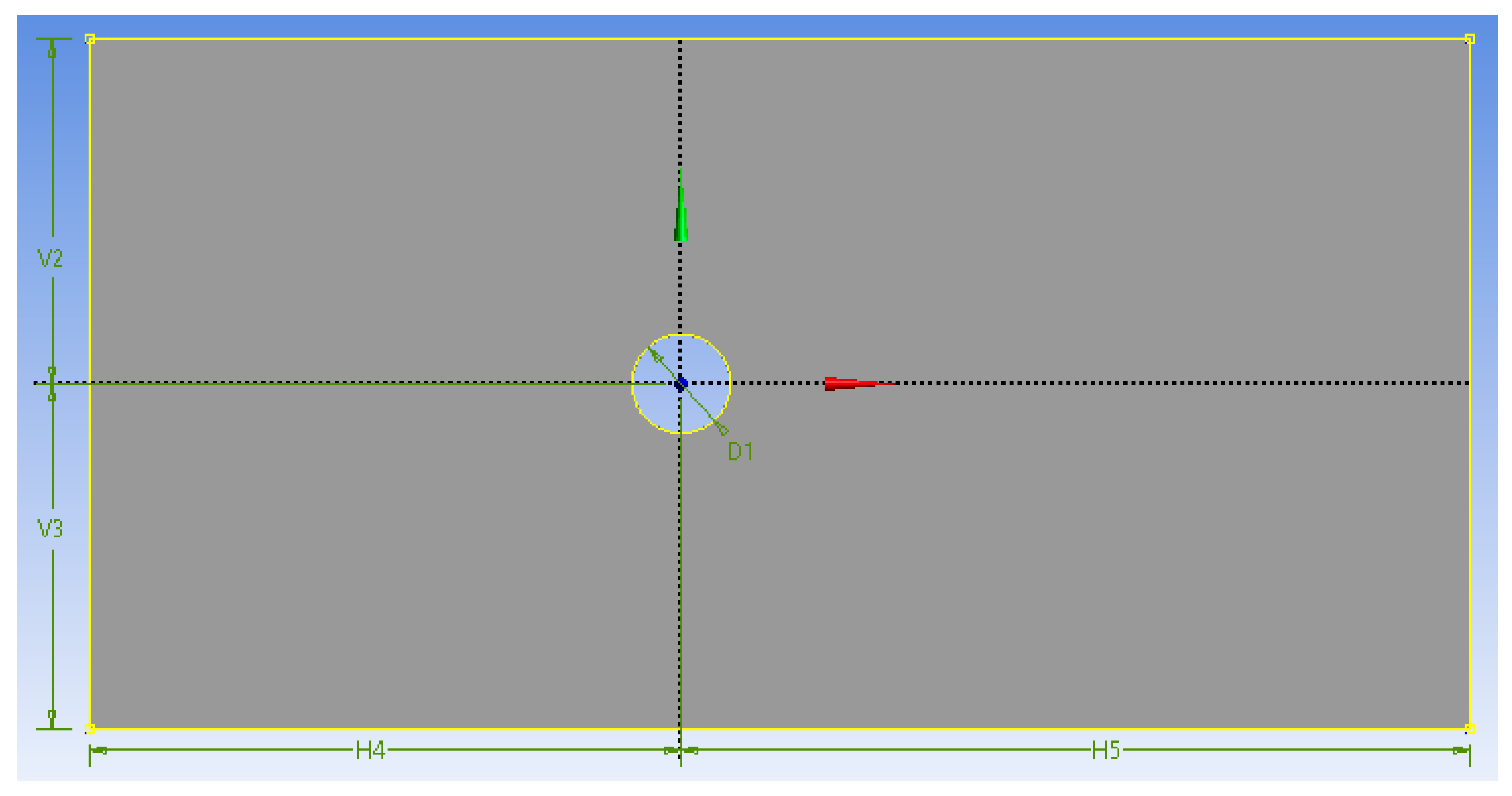
| Parameters | Value | Unit |
|---|---|---|
| Buoy Diameter (D1) | 10 | m |
| Horizontal Height of boundary near inlet to centre of buoy (H4) | 60 | m |
| Horizontal Height of boundary near outlet (H5) | 80 | m |
| Vertical height of boundary from top wall to centre of buoy (V2) | 35 | m |
| Vertical height of boundary from top wall to centre of buoy (V3) | 35 | m |
| Model | Metacentric Height (m) | Buoy Diameter (m) | Buoy Skirt Diameter (m) | Buoy Skirt Width (m) | Responses ** |
|---|---|---|---|---|---|
| A1 | 0.25 | 10.00 | 13.90 | 0.1 | LF + WF |
| A2 | 0.25 | 10.00 | 13.90 | 0.2 | LF + WF |
| A3 | 0.25 | 10.00 | 13.90 | 0.3 | LF + WF |
| B1 | 0.25 | 10.00 | 13.90 | 0.4 | LF + WF |
| B2 | 0.25 | 10.00 | 13.90 | 0.5 | LF + WF |
| B3 | 0.25 | 10.00 | 14.90 | 1.0 | LF + WF |
| C1 | 0.25 | 10.00 | 15.90 | 1.5 | LF + WF |
| C2 | 0.25 | 10.00 | 16.90 | 2.0 | LF + WF |
| C3 | 0.25 | 10.00 | 17.90 | 2.5 | LF + WF |
| D1 | 0.25 | 10.00 | 13.90 | 1.5 | LF + WF |
| D2 | 0.50 | 10.00 | 13.90 | 1.5 | LF + WF |
| D3 | 0.75 | 10.00 | 13.90 | 1.5 | LF + WF |
Publisher’s Note: MDPI stays neutral with regard to jurisdictional claims in published maps and institutional affiliations. |
© 2022 by the authors. Licensee MDPI, Basel, Switzerland. This article is an open access article distributed under the terms and conditions of the Creative Commons Attribution (CC BY) license (https://creativecommons.org/licenses/by/4.0/).
Share and Cite
Amaechi, C.V.; Ye, J. An Investigation on the Vortex Effect of a CALM Buoy under Water Waves Using Computational Fluid Dynamics (CFD). Inventions 2022, 7, 23. https://doi.org/10.3390/inventions7010023
Amaechi CV, Ye J. An Investigation on the Vortex Effect of a CALM Buoy under Water Waves Using Computational Fluid Dynamics (CFD). Inventions. 2022; 7(1):23. https://doi.org/10.3390/inventions7010023
Chicago/Turabian StyleAmaechi, Chiemela Victor, and Jianqiao Ye. 2022. "An Investigation on the Vortex Effect of a CALM Buoy under Water Waves Using Computational Fluid Dynamics (CFD)" Inventions 7, no. 1: 23. https://doi.org/10.3390/inventions7010023
APA StyleAmaechi, C. V., & Ye, J. (2022). An Investigation on the Vortex Effect of a CALM Buoy under Water Waves Using Computational Fluid Dynamics (CFD). Inventions, 7(1), 23. https://doi.org/10.3390/inventions7010023