Solution of Steady Incompressible MHD Problems with Quasi-Least Square Method

Abstract

A quasi-least-squares (QLS) mixed finite element method (MFE) based on the $L^2$-inner product is utilized to solve an incompressible magnetohydrodynamic (MHD) model. These models are associated with the three unknown terms, i.e., fluid velocity, fluid pressure, and magnetic field. For the MHD-based models, common theories and algorithms for approximation of the solutions are not always applicable because of the choice of the functional spaces during the utilization of the weak formulation. It is well known that the spaces used for the approximation of the different unknowns, e.g., the spaces for the unknowns, cannot be chosen independently for the variational formulation, and may have to satisfy strict stability conditions such as the inf-sup, or Ladyzhenskaya–Babuska–Brezzi (LBB) condition. The dependency of the selection of the spaces for the unknowns are critical and always not applicable for some pair of unknowns. Because of this, the numerical or theoretical solutions must have to face some stability issue. The proposed scheme ($L^2$-inner product) is introduced to circumvent this deficiency of the conditions (inf-sup or LBB) and obtained a well-posed solution theoretically. The model equations are nonlinear and highly coupled with the combination of Navier–Stokes and Maxwell relations. First, these nonlinear models are made linear around a specific state wherein the modified system represents an algebraic equation in a first-order symmetric form. Secondly, a direct iteration technique is applied to solve the nonlinearities and obtain a theoretical convergent rate for a general initial guess. Theoretical results show that only a single parameter with a single initial guess is sufficient to establish the well-posedness of the solution.

1. Introduction

Magnetohydrodynamics (MHD) is a combined study of hydrodynamic flows and electromagnetic fluid flow through coupling forces and their interactions. These equations consist of highly coupling equations with well-known Maxwell equations and the hydrodynamic equations for fluid flows. Alfven first proposed the field of MHD for single- and multi-fluid flows [1]. More recently, this field has become important because of its utilization and practical applications in geophysics, astrophysics, and many other engineering fields, like cooling metal, MHD propulsion [2], MHD pumps [3], process metallurgy [4], controlled thermonuclear fusion and seawater propulsion [5], electromagnetic casting of metals, MHD power generation, MHD ion propulsion [6,7] etc. Moreover, the hydrodynamical behavior of conducting fluids, e.g., electrolytes, liquid metal cooling in nuclear reactors [8], and plasmas are usually formulated via MHD models [9]. Furthermore, the theoretical and numerical investigations can be further seen in the following articles and are the given references [10,11,12].

Because these equations are not easily solvable for the analytical solution, the alternative way to solve the complex model equations are the numerical solutions where inf-sup or Ladyzhenskaya–Babuska–Brezzi (LBB) conditions need to satisfy for the well-posedness of the models. The complications caused by the well-known inf-sup condition have prompted the introduction of various stabilization techniques intended to circumvent these conditions [13], a Galerkin method, Galerkin least square method, penalty method, $L^2$-inner products, different stabilization techniques and many modified methods are abundantly used to find the numerical solutions [14,15,16,17], and the well-posedness of the stationary equations with the inf-sup conditions have been given in [18]. MHD-modeled equations are highly non-linear coupling equations which must have to accept the complicated structure of the solution. Therefore, it does require an attractive, efficient numerical scheme which plays a key role to find the solution of such types of complicated structured models. In MFE literature, the least square methods are utilized for such types of complex and non-linear models to find the approximate solution of higher-order PDEs by defining some norms of functional spaces as Hilbert-type to solve [19,20,21,22,23], singular solutions of flows related to viscoelastic behaviours [24], heat transfer and flows [25], and fluids for which temperature-dependecy or viscosity-dependency are critical [17]. Standard least square methods are efficient, effective, and smart enough to give approximate solutions of the non-linear model equations in the linear algebraic form, which would be symmetric and positive-definite. During the last decade, many methods and theories of least square methods have been discussed in the literature. For further details on such applications, we refer interested readers to [26,27,28] among others.

Similarly, a quasi-least-square scheme (QLSFES) is developed [23] to solve the problems in the $L^2$-inner product. Typically, stabilization relies on some form of modification of the discrete continuity equation. For example, in [29] the continuity equation is modified to penalize the stability issue with the addition of a single parameter to make the bilinear form coercive for some specific finite elements. The central point of the scheme is to study the problems in the $L^2$-norm to the Oseen type (linearized) forms of given coupled nonlinear problems. It has several benefits; first, only $L^2$-inner product with norms is used in these methods which are convenient for the computer programming sense. Second, by using the linearizing way (Oseen type), someone can get iterative methods with symmetric positive-definite coefficient metrics. However, this simplified iterative method is easily convergent in a complex domain of initial guess [23,30,31]. For the MHD-based models, common theories and algorithms for approximation of the solutions of such nonlinear problems are not always applicable because of the functional spaces, i.e., Hilbert space for the velocity and pressure. These are not convenient to utilize the Hilbert space, which will ultimately create some stability issue in the analysis. The QLSFES can be easily applied to circumvent this deficiency of the main conditions (inf-sup or LBB). Thus, the prime intention here is to develop a scheme for a coupled branch of non-linear problems to analyze the existence and convergence of model equations. The least-square MFE schemes are inadequate to address the local convergent properties of coupled non-linear problems. However, this method can be utilized as an effective and sufficient way for the well-posedness of the incompressible MHD models without the inf-sup conditons.

In this contribution, the practicality principle can always be met by transforming the given model equations into a transformed first-order system and forming least-squares functionals that use only $L^2$-norms. We focus attention on quasi-least-squares methods for which the discretization step is invoked after the quasi-least-squares functional has been defined. The key point to utilize this setting is that it allows one to point out the variational interpretation of least-squares principles as projections in a Hilbert space with respect to problem-dependent inner products. From this point of view, the principal task in the formulation of the method becomes setting up a least-squares functional that is norm-equivalent ($L^2$-norms) in some Hilbert space. This in turn allows one to work in the variational setting as continuity and coercivity (well-posedness) without the LBB or inf-sup conditions. A quasi-least-squares (QLS) mixed finite element method (MFE) based on the $L^2$-inner product is easily convinced to solve a coupled and nonlinear incompressible magnetohydrodynamic (MHD) model. Here, first, these nonlinear models are made linear around a particular state wherein linearized first-order equations represent an algebraic system of equations with symmetric matrices. Secondly, a direct iteration technique is applied to couple up the nonlinearities and obtain a theoretical convergent rate for general initial guess. As far as we know from the existing literature, this method has never been considered to find the solution of the MHD model equations without the LBB/or inf-sup conditions.

From a theoretical viewpoint, such a bona-fide (continuous) QLS finite element methods possess a number of significant and valuable properties, as follows.

• The weak problems are, in general, coercive.
• Conforming discretizations lead to stable and, ultimately, optimally accurate methods.
• The resulting algebraic problems are symmetric and positive definite.
• Essential boundary conditions may be imposed in a weak sense.
• Finite element spaces of equal interpolation order, defined with respect to the same triangulation, can be used for all unknowns.
• Algebraic problems can be solved by using standard and robust iterative methods, such as conjugate gradient methods.
• Methods can be implemented without any matrix assemblies, even at the element level.
• Only a single parameter with a single initial guess is sufficient to establish the well-posedness of the solution. In the existing literature this is the first time we apply for this model.

The rest of the work is arranged as follows. In Section 2, we demonstrate linear and non-linear incompressible stationary MHD equations with the proposed scheme (QLSFES). In Section 3, we investigate the well-posedness of the developed QLSFES system for investigation of the initial guess. In Section 4, we discuss convergence of the proposed scheme in the case of the nonsingular exact solution. In Section 5, the theoretical is proven and in conclusion the contribution is illustrated to end this work.

2. Model Introduction

This work illustrates the numerical resolution of the stationary-coupled magnetohydrodynamics system of equations [32,33]. The unknowns for this problem are supposed symbolically as velocity field $\overrightarrow{{\mathbf{v}}_f}$, the magnetic field ${\overrightarrow{\mathbf{M}}}_B$, and fluid pressure p under the connected two-dimensional domain $\omega$.

The non-dimensional stationary MHD equations are as follows:

$$\begin{array}{ccc}\hfill \overrightarrow{{\mathbf{v}}_f}·\nabla \overrightarrow{{\mathbf{v}}_f}-\frac{1}{R^e}\eta \overrightarrow{{\mathbf{v}}_f}+\nabla p+S({\overrightarrow{\mathbf{M}}}_B\times \nabla \times \overrightarrow{{\mathbf{M}}_B})& =& \mathbf{f}in\omega ,\hfill \end{array}$$

(1)

$$\begin{array}{ccc}\hfill \nabla ·{\mathbf{v}}_f& =& 0in\omega ,\hfill \end{array}$$

(2)

$$\begin{array}{ccc}\hfill \frac{1}{R^m}\nabla \times (\nabla \times {\overrightarrow{\mathbf{M}}}_B)-S(\nabla \times (\overrightarrow{{\mathbf{v}}_f}\times {\overrightarrow{\mathbf{M}}}_B))& =& 0in\omega ,\hfill \end{array}$$

(3)

$$\begin{array}{ccc}\hfill \nabla ·{\overrightarrow{\mathbf{M}}}_B& =& 0in\omega ,\hfill \end{array}$$

(4)

where $R^e,$ signifies the Reynolds number for hydrodynamic, $R^m$ the Reynolds number for magnetism, and $S=\frac{M^2}{R^e{R}^m}$, with $M>0$, coupling number respectively. In the literature of the industrial sense, we know that, the parameters are considered always $R^e\approx {10}^5$, $R^m\approx {10}^{-1}$ and $S\approx 1$. To acquire the values of the known velocity field $\overrightarrow{{\mathbf{v}}_f}=(v_1,v_2)$ and pressure field p and magnetic field ${\overrightarrow{\mathbf{M}}}_B=(b_1,b_2)$ are given in a bounded domain $\omega$. We consider the load function $\mathbf{f}$ represents the external forces or inertial terms. Additionally, for the 2D form, the operator can be defined as $\nabla \times {\overrightarrow{\mathbf{M}}}_B=\frac{\partial b_2}{\partial x}-\frac{\partial b_1}{\partial y}$, while the product of given vectors $\overrightarrow{{\mathbf{v}}_f}=(v_1,v_2)$ and ${\overrightarrow{\mathbf{M}}}_B=(b_1,b_2)$ is defined as $\overrightarrow{{\mathbf{v}}_f}\times {\overrightarrow{\mathbf{M}}}_B=v_1{b}_2-v_2{b}_1$.

The system of nonlinear stationary MHD can be solved under the set of boundary conditions within the connected domain $\omega \in {\mathbb{R}}^2$ on boundary $\partial \omega$ is given from the references [33,34,35,36]:

$$\begin{array}{ccc}\hfill \overrightarrow{{\mathbf{v}}_f}& =& 0\mathrm{on}\partial \omega ,\hfill \end{array}$$

(5)

$$\begin{array}{ccc}\hfill {\overrightarrow{\mathbf{M}}}_B·\overrightarrow{\mathbf{n}}& =& 0\mathrm{on}\partial \omega ,\hfill \end{array}$$

(6)

$$\begin{array}{ccc}\hfill \nabla \times {\overrightarrow{\mathbf{M}}}_B\times \overrightarrow{\mathbf{n}}& =& 0\mathrm{on}\partial \omega ,\hfill \end{array}$$

(7)

where $\overrightarrow{\mathbf{n}}$ is a normal vector to the domain $\omega$ [17]. Here Equation (5) is representing the viscous nature fluids and is well-known as a no-slip boundary condition, whereas the Equations (6) and (7) are nominated for the perfect conduction wall.

Remark 1.

Alternately, some other boundary constraints are utilized in the literature [12,36,37,38,39] are ${\overrightarrow{\mathit{M}}}_B·\overrightarrow{\mathit{n}}=0$ in Equation (6) and $\nabla \times {\overrightarrow{\mathit{M}}}_B\times \overrightarrow{\mathit{n}}=0$ in Equation (7) for the unknown ${\overrightarrow{\mathit{M}}}_B$. We utilize ${\overrightarrow{\mathit{M}}}_B\times \overrightarrow{\mathit{n}}=0$ and $\overrightarrow{\mathit{n}}\times (\nabla \times {\overrightarrow{\mathit{M}}}_B)=0$, which is given for the nonlinear MHD for a single-fluid flow.

3. Quasi-Least-Square MFE

In this section, we discuss the QLES based on the $L^2$-inner product with MFE for the stationary MHD models.

3.1. Definitions and Notations

Here, the following Sobolev spaces are introduced first. Let us consider $C^{\infty }\left(\omega \right)$ to be the set of infinitely differentiable continuous functions $C_0^{\infty }\left(\omega \right)=\{\mathbf{o},{\mathbf{M}}_B\in C^{\infty }\left(\omega \right)\}$; the vector-support functions $\mathbf{o},{\mathbf{M}}_B$ are in domain $\omega$. (In the coming sections, we suppose o, ${\mathbf{M}}_B$ Oseen type iterative values utilizing for the conversion of the non-linear to linearization of the MHD model equations). Moreover, the Sobolev function spaces in standard form are given as:

$$\begin{array}{ccc}\hfill \mathfrak{W}:& =& {\left[H^1\left(\omega \right)\right]}^{n\times n},\hfill \\ \hfill \mathbf{I}:& =& H_0^1{\left(\omega \right)}^n,\hfill \\ \hfill \mathbf{P}:& =& \{q\in H^1\left(\omega \right);{\int }_{\omega }qd\omega =0\},\hfill \\ \hfill \mathbf{Y}:& =& H_0^1\left(\omega \right),\hfill \\ \hfill \mathbf{N}:& =& {\left[H^1\left(\omega \right)\right]}^n.\hfill \end{array}$$

Let $\mathfrak{V}={\left(V_{ij}\right)}_{n\times n}=({\overrightarrow{{\mathbf{v}}_f}}_1,{\overrightarrow{{\mathbf{v}}_f}}_2\cdots ,{\overrightarrow{{\mathbf{v}}_f}}_n)$ be known as a vector function of degree $n\times n$ with column matrices ${\overrightarrow{{\mathbf{v}}_f}}_k$, $1\le k\le n$. For each n-dimensional matrix $\overrightarrow{{\mathbf{v}}_f}$ and vector $\mathfrak{U}$, introduce $\nabla \overrightarrow{{\mathbf{v}}_f}=(v_1,v_2\cdots ,v_n)$ and $\nabla \times \mathfrak{U}=(\nabla \times {\overrightarrow{{\mathbf{v}}_f}}_1,\nabla \times {\overrightarrow{{\mathbf{v}}_f}}_2\cdots ,\nabla \times {\overrightarrow{{\mathbf{v}}_f}}_n)$, $\nabla ·{\mathfrak{U}}^T={(\nabla ·{\overrightarrow{{\mathbf{v}}_f}}_1,\nabla ·{\overrightarrow{{\mathbf{v}}_f}}_2\cdots ,\nabla ·{\overrightarrow{{\mathbf{v}}_f}}_n)}^T$ and similarly $\mathbf{B}=\nabla \times {\overrightarrow{\mathbf{M}}}_B$. For the conciseness and applicability of the QLS method, the first-order system of equations can be now equivalently written as:

3.2. The Stationary First Order MHD Model and QLSFE Scheme Algorithms

An algorithm is proposed to solve the incompressible stationary MHD Model (1)–(4) via the following first order system as following:

$$\begin{array}{ccc}\hfill -\nu \nabla ·{\mathfrak{U}}^T+(\overrightarrow{{\mathbf{v}}_f}·\nabla )\overrightarrow{{\mathbf{v}}_f}+\nabla p+S({\overrightarrow{\mathbf{M}}}_B\times \nabla \times {\overrightarrow{\mathbf{M}}}_B)& =& \mathbf{f}\mathrm{in}\omega ,\hfill \end{array}$$

(8)

$$\begin{array}{ccc}\hfill \mathfrak{U}-\nabla \overrightarrow{{\mathbf{v}}_f}& =& 0\mathrm{in}\omega ,\hfill \end{array}$$

(9)

$$\begin{array}{ccc}\hfill \nabla ·\overrightarrow{{\mathbf{v}}_f}& =& 0\mathrm{in}\omega ,\hfill \end{array}$$

(10)

$$\begin{array}{ccc}\hfill {\nu }_m\nabla \times \left(\mathbf{B}\right)-S(\nabla \times (\overrightarrow{{\mathbf{v}}_f}\times {\overrightarrow{\mathbf{M}}}_B))& =& 0\mathrm{in}\omega ,\hfill \end{array}$$

(11)

$$\begin{array}{ccc}\hfill \mathbf{B}-\nabla \times {\overrightarrow{\mathbf{M}}}_B& =& 0\mathrm{in}\omega ,\hfill \end{array}$$

(12)

$$\begin{array}{ccc}\hfill \nabla ·{\overrightarrow{\mathbf{M}}}_B& =& 0\mathrm{in}\omega .\hfill \end{array}$$

(13)

In the further formulation for any $\mathbf{o},{\overrightarrow{\mathbf{M}}}_B\in \mathbf{I}$ is considered from the Oseen type formulation [23,30] where o and ${\overrightarrow{\mathbf{M}}}_B$ are known functions usually chosen from the previous iterative step of the Picard iterations which are always known values for the next iteration and are also supposed regular for the unknown values. We represent the viscosity of the hydrodynamic $\nu =\frac{1}{R^e}$, and the diffusivity of the magnetism ${\nu }^m=\frac{1}{R^m}$. Then the bilinear form of the functions are now introduced for the ($\mathfrak{V},\overrightarrow{{\mathbf{v}}_f},p,\mathbf{B},{\overrightarrow{\mathbf{M}}}_B$) and ($\mathfrak{W},\rho ,q,\tau ,\mathbf{c}$) respectively ($\mathfrak{W}\times \mathbf{I}\times \mathbf{P}\times \mathbf{Y}\times \mathbf{N}$) as

$$\begin{array}{cc}\hfill \mathcal{L}(\mathbf{o},{\overrightarrow{\mathbf{M}}}_B;(\mathfrak{U},& \overrightarrow{{\mathbf{v}}_f},p,\mathbf{B},{\overrightarrow{\mathbf{M}}}_B),(\mathfrak{W},\rho ,q,\tau ,\sigma ))\hfill \\ \hfill & =(-\nu \nabla ·{\mathfrak{V}}^T+(\mathbf{o}·\nabla )\overrightarrow{{\mathbf{v}}_f}+\nabla p+S({\overrightarrow{\mathbf{M}}}_B\times \nabla \times {\overrightarrow{\mathbf{M}}}_B),\hfill \\ \hfill & -\nu \nabla ·{\mathfrak{W}}^T+(\mathbf{o}·\nabla )\rho +\nabla q+S({\overrightarrow{\mathbf{M}}}_B\times \nabla \times \sigma ))\hfill \\ \hfill & +(\mathfrak{V}-\nabla \overrightarrow{{\mathbf{v}}_f},\mathfrak{W}-\nabla \rho )+{\gamma }^2(\nabla ·\overrightarrow{{\mathbf{v}}_f},\nabla ·\rho )\hfill \\ \hfill & +({\nu }_m\nabla \times \mathbf{B}-\nabla \times )(\overrightarrow{{\mathbf{v}}_f}\times {\overrightarrow{\mathbf{M}}}_B),{\nu }_m(\nabla \times \tau -\nabla \times (\rho \times {\overrightarrow{\mathbf{M}}}_B))\hfill \\ \hfill & +(\mathbf{B}-\nabla \times {\overrightarrow{\mathbf{M}}}_B,\tau -\nabla \times \sigma )+{\eta }^2(\nabla ·{\overrightarrow{\mathbf{M}}}_B,\nabla ·\sigma )\hfill \end{array}$$

(14)

where the two positive constants $\gamma$ and $\eta$ are to be found in the upcoming sections. Suppose that $(\overrightarrow{{\mathbf{v}}_f},p,{\overrightarrow{\mathbf{M}}}_B)$ are the solutions of system Equations (1)–(4) which are in ${\left[H^2\left(\omega \right)\right]}^d\times H^1\left(\omega \right)\times H^2\left(\omega \right)$. Let us consider $\mathfrak{V}=\nabla \overrightarrow{{\mathbf{v}}_f}$ and $\mathbf{B}=\nabla \times {\overrightarrow{\mathbf{M}}}_B$, and now the solution of unknown variables ($\mathfrak{V},\overrightarrow{{\mathbf{v}}_f},p,\mathbf{B},{\overrightarrow{\mathbf{M}}}_B$) satisfies the following QLS variational formulation:

$$\begin{array}{cc}\hfill \mathcal{L}(\overrightarrow{{\mathbf{v}}_f},& {\overrightarrow{\mathbf{M}}}_B;(\mathfrak{V},\overrightarrow{{\mathbf{v}}_f},p,\mathbf{B},{\overrightarrow{\mathbf{M}}}_B),(\mathfrak{W},\rho ,q,\tau ,\sigma ))\hfill \\ \hfill & =(f,-\nu \nabla ·{\mathfrak{W}}^T+\overrightarrow{{\mathbf{v}}_f}·\nabla \rho +\nabla q+S({\overrightarrow{\mathbf{M}}}_B\times \nabla \times \sigma ))\hfill \\ \hfill & \forall (\mathfrak{W},\rho ,q,\tau ,\sigma )\in \mathfrak{W}\times \mathbf{I}\times \mathbf{P}\times \mathbf{Y}\times \mathbf{N}.\hfill \end{array}$$

(15)

3.3. Variational Form of the MHD

For the mathematical solutions and findings, few symbols utilized in functional spaces are introduced. Suppose that $W^{m,p}\left(G\right)$ is noted particularly written as $H^m\left(\omega \right)$ with the norm $\mid \mid ·\mid {\mid }_m$ and seminorm ${|·|}_m$ [40,41] for $p=2$ and $m=0$ then $W_2^0\left(\omega \right).$ We see that the inner product is always given by $(·,·)$, $\mid \mid ·\mid \mid =\mid \mid ·\mid {\mid }_0$ for the space $L^2\left(\omega \right)$ respectively, and the general norm for this space can be written as $L^p\left(\omega \right)$ norm, which is equivalent to $\mid \mid ·\mid {\mid }_{L^p}$, with some notable cases of Hilbert space $L^2\left(\omega \right)=\mid \mid ·\mid {\mid }_{L^2\left(\omega \right)}$ and the Banach space $L^{\infty }\left(\omega \right)=\mid \mid ·\mid {\mid }_{\infty }$. Here G is ignored for $G=\omega$ without any confusion for the notational simplicity.

However, with the above setting, the corresponding variational formulation, we introduce FE spaces (${\mathfrak{W}}^h\times {\mathbf{I}}^h\times {\mathbf{P}}^h\times {\mathbf{Y}}^h\times {\mathbf{N}}^h)\subset (\mathfrak{W}\times \mathbf{I}\times \mathbf{P}\times \mathbf{Y}\times \mathbf{N}$) on the triangular elements $T^h$ where $T^h$ is a member of FE triangulations of the discretized domain $\omega$ and script h represents the largest element in the meshed domain or the triangles. By considering the QLS illustration, we can write:

QLSFES. Find (${\mathfrak{V}}^h,{\overrightarrow{{\mathbf{v}}_f}}^h,p^h,{\mathbf{B}}^h,{\overrightarrow{\mathbf{M}}}_B^h)\in ({\mathfrak{W}}^h\times {\mathbf{I}}^h\times {\mathbf{P}}^h\times {\mathbf{Y}}^h\times {\mathbf{N}}^h$) such that

$$\begin{array}{cc}\hfill \mathcal{L}& \left({\overrightarrow{{\mathbf{v}}_f}}^h,{\overrightarrow{\mathbf{M}}}_B^h;({\mathfrak{V}}^h,{\overrightarrow{{\mathbf{v}}_f}}^h,p^h,{\mathbf{B}}^h,{\overrightarrow{\mathbf{M}}}_B^h),({\mathfrak{W}}^h,{\rho }^h,q^h,{\tau }^h,{\sigma }^h)\right)\hfill \\ \hfill & =\left(f,-\nu \nabla ·{\mathfrak{W}}^h+{\overrightarrow{{\mathbf{v}}_f}}^h·\nabla {\rho }^h+\nabla q^h+S({\overrightarrow{\mathbf{M}}}_B^h\times \nabla \times {\sigma }^h)\right)\hfill \\ & \forall ({\mathfrak{W}}^h,{\rho }^h,q^h,{\tau }^h,{\sigma }^h)\in ({\mathfrak{W}}^h\times {\mathbf{I}}^h\times {\mathbf{P}}^h\times {\mathbf{Y}}^h\times {\mathbf{N}}^h).\hfill \end{array}$$

(16)

Remark 2.

QLSFES is a simple symmetric form. For practical calculation, we define two parameters γ and η with the incompressibility conditions. These parameters are important to ensure the coercivity and continuity of the scheme. Indeed, it is not possible to ensure the coerciveness of the bilinear form of $L(\mathbf{o},{\overrightarrow{\mathbf{M}}}_B:·,·)$ for each $\mathbf{o},{\overrightarrow{\mathbf{M}}}_B\in \mathbf{I}$. But, by choosing suitable values for γ and η they became well-defined and positive symmetric in some bounded domain which holds the solution of (1)–(4). In the next sections, we will discuss the judicious guess of the parameters γ and η for the linear form. The ideal feature of this technique is that a solution of a nonlinear model equation can be obtain without any initial guess for the iterative procedure for a large domain. We confirm this feature in forthcoming formulations in our analysis part.

4. QLSFES Convergence and Existence of the Solutions

In this section, we obtain convergence and existence of the solution of proposed scheme with the illustration of four steps.

• We demonstrate property of the $L(\mathbf{o},{\overrightarrow{\mathbf{M}}}_B:·,·)$ bilinear function. For any parameter $\gamma$ and $\eta$ are introduced in such a way that there exists a bounded function set $L(\mathbf{o},{\overrightarrow{\mathbf{M}}}_B:·,·)$ that is well defined and continuous as $\mathbf{o}$ and ${\overrightarrow{\mathbf{M}}}_B$ holds in this bounded domain.
• In step two, we find out a large domain of bounded functions which holds all solutions of the System (8)–(13). We intend to solve the nonlinear coupled equations by the right choice of $\gamma$ and $\eta$,and $L(\mathbf{o},{\overrightarrow{\mathbf{M}}}_B:·,·)$ is well-defined as $\mathbf{o}$ and ${\overrightarrow{\mathbf{M}}}_B$ are in this large domain of functions.
• To show the well-posedness of the proposed scheme QLSFES, we establish the nonlinear plan of the scheme in such a way that the solutions under some nominated domain are fixed points. In step one and step two, we summarize that for a specific value of $\eta$ and $\gamma$, the system of the nonlinear model is distinctively executable in this specific bounded set (see detail in Lemmas 3 and 4). Moreover, in Theorem 1, by using the fixed point theory [23], we illustrate briefly the existence of solutions of the scheme.
• In the fourth step, Theorem 2 is given to illustrate the convergence and existence of the proposed scheme QLSFES.
  Before proceeding to the actual contribution, we intend to understand several existing results which are utilized in the immanent sections. By the theory of embedding and the Poincaré’s inequality, the positive constants e, $a_0$, and $a_1$ always depend on the fact that the domain can be recalled as

$$\begin{array}{ccc}\hfill a_0{\Vert \mathbf{u}\Vert }_{L^4}^2& \le & {\Vert \nabla \mathbf{u}\Vert }_{L^2\left(\omega \right)}^2,\hfill \\ \hfill a_1{\Vert \mathbf{u}\Vert }_1^2& \le & {\Vert \nabla \mathbf{u}\Vert }_{L^2\left(\omega \right)}^2,\forall \mathbf{u}\in \mathbf{I}.\hfill \\ \hfill \Vert \overrightarrow{{\mathbf{v}}_f}{\Vert }_{L^4}^2& \le & e\Vert \overrightarrow{{\mathbf{v}}_f}{\Vert }_1^2\forall \overrightarrow{{\mathbf{v}}_f}\in \mathbf{I}.\hfill \end{array}$$

(17)

$$\begin{array}{ccc}\hfill \Vert {\overrightarrow{\mathbf{M}}}_B{\Vert }_{L^2\left(\omega \right)}^2& \le & a_2(\Vert \nabla \times {\overrightarrow{\mathbf{M}}}_B{\Vert }_{L^2\left(\omega \right)}^2+\Vert \nabla ·{\overrightarrow{\mathbf{M}}}_B{\Vert }_{L^2\left(\omega \right)}^2),\forall {\overrightarrow{\mathbf{M}}}_B\in \mathbf{N}\hfill \\ \hfill \Vert {\overrightarrow{\mathbf{M}}}_B{\Vert }_{L^4}^2& \le & C\Vert {\overrightarrow{\mathbf{M}}}_B{\Vert }_1^2\hfill \end{array}$$

(18)

$$\begin{array}{ccc}\hfill \Vert \nabla \times {\overrightarrow{\mathbf{M}}}_B{\Vert }_{L^2\left(\omega \right)}^2& \le & a_3{\Vert {\overrightarrow{\mathbf{M}}}_B\Vert }_1^2\hfill \end{array}$$

(19)

$$\begin{array}{ccc}\hfill \Vert {\overrightarrow{\mathbf{M}}}_B{\Vert }_{L^2\left(\omega \right)}^2& \le & e\Vert \nabla \times {\overrightarrow{\mathbf{M}}}_B{\Vert }_{L^2\left(\omega \right)}^2\hfill \end{array}$$

(20)

$$\begin{array}{ccc}& \le & e\Vert {\overrightarrow{\mathbf{M}}}_B{\Vert }_{L^2\left(\omega \right)}^2\hfill \end{array}$$

(21)

According to Green’s formula and integration by parts [42], we can state

$$\begin{array}{ccc}\hfill (\nabla \overrightarrow{{\mathbf{v}}_f},\mathbf{u})-(\overrightarrow{{\mathbf{v}}_f},\nabla \mathbf{u})& =& 0,\forall \overrightarrow{{\mathbf{v}}_f},\mathbf{u}\in \mathbf{I}\hfill \\ \hfill (\mathbf{o}·\nabla \mathbf{u},\mathbf{u})+\frac{1}{2}(div\mathbf{o},\mid \mathbf{u}{\mid }^2)& =& 0,\forall \mathbf{u},\mathbf{o}\in \mathbf{I}\hfill \\ \hfill ({\overrightarrow{\mathbf{M}}}_B\times \nabla \times {\overrightarrow{\mathbf{M}}}_B,\mathbf{u})-(\overrightarrow{{\mathbf{v}}_f}\times {\overrightarrow{\mathbf{M}}}_B,\nabla \times {\overrightarrow{\mathbf{M}}}_B)& =& 0,\forall \mathbf{u}\in \mathbf{I},\forall {\overrightarrow{\mathbf{M}}}_B,{\overrightarrow{\mathbf{M}}}_B\in \mathbf{N}\hfill \\ \hfill \Vert \mathbf{o}\times {\overrightarrow{\mathbf{M}}}_B{\Vert }_{L^2\left(\omega \right)}^2& \le & {e\Vert \mathbf{o}\Vert }_{L^{\infty }}^2{\Vert {\overrightarrow{\mathbf{M}}}_B\Vert }_{L^2\left(\omega \right)}^2\forall \mathbf{o},{\overrightarrow{\mathbf{M}}}_B\in \left(L^2{\left(\omega \right)}^{n\times n}\right).\hfill \end{array}$$

(22)

The bilinear form $(·,·)$ is well known as an inner product in space $L^2\left(\omega \right)$ or $L^2{\left(\omega \right)}^n$. It is always known to be a fact that $q\in L^2\left(\omega \right)$ holds the boundary condition $(q,1)=0$ if $\varphi \in {\left[H_0^1\left(\omega \right)\right]}^n$ such that

$$\begin{array}{ccc}\hfill div·\varphi & =& q,\hfill \\ \hfill {\Vert \varphi \Vert }_1& \le & C_e{\Vert q\Vert }_{L^2\left(\omega \right)}.\hfill \end{array}$$

(23)

Lemma 1.

Let constants $K_o>0,0<\eta <2a_{0}min(\nu ,\frac{{\nu }^m}{2})$ and $\gamma >max(K_o,1)$. There exists two constants β and $\beta \ast$ such that for each $\mathit{o}\in \mathit{I},{\mathit{b}}_M\in \mathit{N}$ satisfying ${\Vert \nabla \mathbf{o}\Vert }_{L^2\left(\omega \right)}\le K_o$ and ${\Vert \nabla ·\mathbf{o}\Vert }_{L^2\left(\omega \right)}\le \eta$, $\Vert {\overrightarrow{\mathit{M}}}_B{\Vert }_{L^{\infty }}\le \pi$ and for each $({\mathfrak{W}}^h,{\mathbf{u}}^h,q^h,{\tau }^h,{\sigma }^h)\in (\mathfrak{W},\mathit{I},\mathit{P},\mathit{Y},\mathit{N})$,

$$\begin{array}{ccc}\hfill \left(i\right)\beta \left[\Vert \nabla \overrightarrow{\mathbf{u}}{\Vert }_{L^2\left(\omega \right)}^2+{\Vert \nabla \times \sigma \Vert }_{L^2\left(\omega \right)}^2\right]& \le & \mathcal{L}\left(\mathbf{o},{\overrightarrow{\mathbf{M}}}_B;(\mathfrak{W},\overrightarrow{{\mathbf{u}}_f},q,\tau ,\sigma ),(\mathfrak{W},\overrightarrow{{\mathbf{u}}_f},q,\tau ,\sigma )\right),\hfill \\ \hfill \left(ii\right)\mathsf{\Lambda }{\mathsf{\Lambda }}^{*}\left[{\Vert \mathfrak{W}\Vert }_{L^2\left(\omega \right)}^2+{\Vert \tau \Vert }_{L^2\left(\omega \right)}^2+{\Vert q\Vert }_{L^2\left(\omega \right)}^2\right]& \le & \mathcal{L}\left(\mathbf{o},{\overrightarrow{\mathbf{M}}}_B;(\mathfrak{W},\overrightarrow{{\mathbf{u}}_f},q,\tau ,\sigma ),(\mathfrak{W},\overrightarrow{{\mathbf{u}}_f},q,\tau ,\sigma )\right),\hfill \end{array}$$

(24)

where the constants $\mathsf{\Lambda }$ and ${\mathsf{\Lambda }}^{*}$ are defined as follows

$$\begin{array}{ccc}\hfill \mathsf{\Lambda }& =& min({\mathsf{\Lambda }}_1,{\mathsf{\Lambda }}_2,{\mathsf{\Lambda }}_3,{\mathsf{\Lambda }}_4,{\mathsf{\Lambda }}_5),where{\mathsf{\Lambda }}_j,1\le j\le 5,\hfill \end{array}$$

(25)

and ${\mathsf{\Lambda }}^{*}=min\left(\frac{1}{2(1+\mathsf{\Lambda })},\frac{1}{2{\left(C_e\right)}^2\mathsf{\Lambda }},\frac{1}{4{\nu }^2{C}_e^2(1+\mathsf{\Lambda })},\frac{a_0^2{a}_1}{2C_e^2{(\eta +K)}^2{a}_1}\right)$.

Proof. 

From Young’s inequality and the given conditions, we can demonstrate

$$\begin{array}{cc}\hfill \Vert \nabla \overrightarrow{{\mathbf{u}}_f}{\Vert }_{L^2\left(\omega \right)}^2& =(\nabla \overrightarrow{{\mathbf{u}}_f}-\mathfrak{W},\nabla \overrightarrow{{\mathbf{u}}_f})+{\nu }^{-1}\left[(-\nu \nabla ·{\mathfrak{W}}^T+(\mathbf{o}·\nabla )\overrightarrow{{\mathbf{u}}_f}+\nabla q+S{\overrightarrow{\mathbf{M}}}_B\times \nabla \times \sigma ,\overrightarrow{{\mathbf{u}}_f})\right]\hfill \\ \hfill & +\left[\frac{1}{2\nu }(\nabla ·\mathbf{o}\overrightarrow{{\mathbf{u}}_f},\overrightarrow{{\mathbf{u}}_f})\right]+{\nu }^{-1}(q,\nabla ·\overrightarrow{{\mathbf{u}}_f})+{\nu }^{-1}\left[(S{\overrightarrow{\mathbf{M}}}_B\times \nabla \times \sigma ,\overrightarrow{{\mathbf{u}}_f})\right]\hfill \\ \hfill & \le \frac{1}{2a_1^2{ϵ}_0{\nu }^2}{\Vert -\nu \nabla ·{\mathfrak{W}}^T+(\mathbf{o}·\nabla )\overrightarrow{{\mathbf{u}}_f}+\nabla q+S{\overrightarrow{\mathbf{M}}}_B\times \nabla \times \sigma \Vert }_{L^2\left(\omega \right)}^2\hfill \\ \hfill & +\frac{1}{2{ϵ}_0}\Vert \nabla \overrightarrow{{\mathbf{u}}_f}{-\mathfrak{W}\Vert }_{L^2\left(\omega \right)}^2+\frac{{\gamma }^2}{4{ϵ}_1}\Vert \nabla ·\overrightarrow{{\mathbf{u}}_f}{\Vert }_{L^2\left(\omega \right)}^2+\frac{{ϵ}_1}{{\gamma }^2{\nu }^2}{\Vert q\Vert }_{L^2\left(\omega \right)}^2\hfill \end{array}$$

(26)

$$\begin{array}{cc}& +(2{ϵ}_0+\frac{\eta }{2{\nu }^2{a}_0})\Vert \nabla \overrightarrow{{\mathbf{u}}_f}{\Vert }_{L^2\left(\omega \right)}^2+\frac{S^2{\pi }^2}{4{\nu }^2{a}_0{ϵ}_0}{\Vert \nabla \times \sigma \Vert }_{L^2\left(\omega \right)}^2\hfill \end{array}$$

(27)

and

$$\begin{array}{ccc}\hfill {\Vert \mathfrak{W}\Vert }_{L^2\left(\omega \right)}^2& \le & 2\left[\Vert \nabla \overrightarrow{{\mathbf{u}}_f}{\Vert }_{L^2\left(\omega \right)}^2+{\Vert \nabla \overrightarrow{{\mathbf{u}}_f}-\mathfrak{W}\Vert }_{L^2\left(\omega \right)}^2\right].\hfill \end{array}$$

(28)

Let us consider $\varphi$ holds (23), and we obtain the following estimation

$$\begin{array}{cc}\hfill {\Vert q\Vert }_{L^2}^2& =-(-\nu \nabla ·{\mathfrak{W}}^T+(\mathbf{o}·\nabla )\overrightarrow{{\mathbf{u}}_f}+\nabla q+S{\overrightarrow{\mathbf{M}}}_B\times \nabla \times \sigma ,\varphi )\hfill \\ \hfill & +\nu (\mathfrak{W},\nabla \varphi )+\left((\mathbf{o}·\nabla )\overrightarrow{{\mathbf{u}}_f}+S{\overrightarrow{\mathbf{M}}}_B\times \nabla \times \sigma ,\varphi \right)\hfill \\ \hfill & \le [\Vert (-\nu \nabla ·{\mathfrak{W}}^T+(\mathbf{o}·\nabla )\overrightarrow{{\mathbf{u}}_f}+\nabla q+S{\overrightarrow{\mathbf{M}}}_B\times \nabla \times \sigma ){\Vert }_{L^2\left(\omega \right)}\hfill \\ \hfill & +{\nu \Vert \mathfrak{W}\Vert }_{L^2\left(\omega \right)}+\frac{1}{a_0}{(\Vert \nabla ·\mathbf{o}\Vert }_{L^2\left(\omega \right)}+{\Vert \nabla \mathbf{o}\Vert }_{L^2\left(\omega \right)})\Vert \nabla \overrightarrow{{\mathbf{u}}_f}{\Vert }_{L^2\left(\omega \right)}{+S\pi \Vert \nabla \times \sigma \Vert }_{L^2\left(\omega \right)}]{\Vert \varphi \Vert }_{H^1}.\hfill \end{array}$$

(29)

By utilizing Equation (23), we can state

$$\begin{array}{cc}\hfill {\Vert q\Vert }_{L^2}^2& \le 2C_{L^2\left(\omega \right)}^2[{\Vert -\nu \nabla ·{\mathfrak{W}}^T+(\mathbf{o}·\nabla )\overrightarrow{{\mathbf{u}}_f}+\nabla q+S{\overrightarrow{\mathbf{M}}}_B\times \nabla \times \sigma \Vert }_{L^2\left(\omega \right)}^2\hfill \\ \hfill & +{\nu }^2{\Vert \mathfrak{W}\Vert }_{L^2\left(\omega \right)}^2+\frac{{(\eta +K)}^2}{a_0^2}\Vert \nabla \overrightarrow{{\mathbf{u}}_f}{\Vert }_{L^2\left(\omega \right)}^2+S^2{\pi }^2{\Vert \nabla \times \sigma \Vert }_{L^2\left(\omega \right)}^2],\hfill \end{array}$$

(30)

in a similar way,

$$\begin{array}{cc}\hfill {\Vert \nabla \times \sigma \Vert }_{L^2\left(\omega \right)}^2=& (\nabla \times \sigma ,\nabla \times \sigma -\tau )+{\nu }_m^{-1}(\sigma ,{\nu }_m\nabla \times \tau -\nabla \times (\overrightarrow{{\mathbf{u}}_f}\times {\overrightarrow{\mathbf{M}}}_B))\hfill \\ \hfill & +{\nu }_m^{-1}(\sigma ,\nabla \times (\overrightarrow{{\mathbf{u}}_f}\times {\overrightarrow{\mathbf{M}}}_B))\hfill \end{array}$$

(31)

$$\begin{array}{cc}\hfill {\Vert \nabla \times \sigma \Vert }_{L^2\left(\omega \right)}^2& \le {4\Vert \nabla \times \sigma -\tau \Vert }_{L^2\left(\omega \right)}^2+\frac{4\nu {}_m{a}_2}{\nu {{}_m}^2{a}_2-\eta }{\Vert {\nu }_m\nabla \times \tau -\nabla \times (\overrightarrow{{\mathbf{u}}_f}\times {\overrightarrow{\mathbf{M}}}_B)\Vert }_{L^2\left(\omega \right)}^2\hfill \\ \hfill & +\frac{2{\pi }^2}{{\nu }_m^2}\Vert \nabla \overrightarrow{{\mathbf{u}}_f}{\Vert }_{L^2\left(\omega \right)}^2+\frac{1}{4}{\Vert \nabla ·\sigma \Vert }_{L^2\left(\omega \right)}^2.\hfill \end{array}$$

(32)

By substituting Equations (30) and (32) in Equation (26), we have

$$\begin{array}{cc}\hfill \Vert \nabla \overrightarrow{{\mathbf{u}}_f}{\Vert }_{L^2}^2& \le \frac{1}{2a_1^2{ϵ}_0{\nu }^2}{\Vert (-\nu \nabla ·{\mathfrak{W}}^T+(\mathbf{o}·\nabla )\overrightarrow{{\mathbf{u}}_f}+\nabla q+S{\overrightarrow{\mathbf{M}}}_B\times \nabla \times \sigma )\Vert }_{L^2}^2\hfill \\ \hfill & +\frac{1}{2{ϵ}_0}\Vert \nabla \overrightarrow{{\mathbf{u}}_f}{-\mathfrak{W}\Vert }_{L^2\left(\omega \right)}^2+\frac{{\gamma }^2}{4{ϵ}_1}\Vert \nabla ·\overrightarrow{{\mathbf{u}}_f}{\Vert }_{L^2\left(\omega \right)}^2+({ϵ}_0+\frac{\eta }{2\nu a_0}){\Vert \nabla \overrightarrow{{\mathbf{u}}_f}\Vert }_{L^2\left(\omega \right)}^2\hfill \\ \hfill & +\frac{a_2{S}^2}{4{\nu }^2{ϵ}_1}\Vert {\nu }_m\nabla \times \tau -\nabla \times (\overrightarrow{{\mathbf{u}}_f}\times {\overrightarrow{\mathbf{M}}}_B){\Vert }_{L^2\left(\omega \right)}^2+2{ϵ}_1{\Vert \nabla \times \sigma \Vert }_{L^2\left(\omega \right)}^2\hfill \\ \hfill & +{ϵ}_1{\Vert \nabla ·\sigma \Vert }_{L^2\left(\omega \right)}^2+\frac{S^2{\nu }_m^2}{4{\nu }^2{ϵ}_1}{\Vert \nabla \times \sigma -\tau \Vert }_{L^2\left(\omega \right)}^2\hfill \\ \hfill & +\frac{2{ϵ}_1{C}_{L^2\left(\omega \right)}^2}{{\gamma }^2{\nu }^2}[{\Vert -\nu \nabla ·{\mathfrak{W}}^T+(\mathbf{o}·\nabla )\overrightarrow{{\mathbf{u}}_f}+\nabla q+S{\overrightarrow{\mathbf{M}}}_B\times \nabla \times \sigma \Vert }^2\hfill \\ \hfill & +{\nu }^2{\Vert \mathfrak{W}\Vert }_{L^2\left(\omega \right)}^2+\frac{{(\eta +K)}^2}{a_0^2}\Vert \nabla \overrightarrow{{\mathbf{u}}_f}{\Vert }_{L^2\left(\omega \right)}^2+S^2{\pi }^2{\Vert \nabla \times \sigma \Vert }_{L^2\left(\omega \right)}^2]\hfill \\ \hfill & \le \left(\frac{1}{2a_1^2{ϵ}_0{\nu }^2}+\frac{2{ϵ}_1{C}_{L^2\left(\omega \right)}^2}{{\gamma }^2{\nu }^2}\right){\Vert (-\nu \nabla ·{\mathfrak{W}}^T+(\mathbf{o}·\nabla )\overrightarrow{{\mathbf{u}}_f}+\nabla q+S{\overrightarrow{\mathbf{M}}}_B\times \nabla \times \sigma )\Vert }_{L^2}^2\hfill \\ \hfill & +\left(\frac{4{ϵ}_1{C}_0^2}{{\gamma }^2}+\frac{1}{2{ϵ}_0}\right)\Vert \nabla \overrightarrow{{\mathbf{u}}_f}{-\mathfrak{W}\Vert }_{L^2\left(\omega \right)}^2+\frac{{\gamma }^2}{4{ϵ}_1}{\Vert \nabla ·\overrightarrow{{\mathbf{u}}_f}\Vert }^2\hfill \\ \hfill & +\left({ϵ}_0+\frac{\eta }{2\nu a_0}+\frac{2{ϵ}_1{C}_0^2{(\eta +K_o)}^2}{{\gamma }^2{\nu }^2{a}_0^2}+\frac{4{ϵ}_1{C}_0^2}{{\gamma }^2}\right){\Vert \nabla \overrightarrow{{\mathbf{u}}_f}\Vert }_{L^2\left(\omega \right)}^2\hfill \\ \hfill & +\left(\frac{2{ϵ}_1{C}_0^2{S}^2{\pi }^2}{{\gamma }^2{\nu }^2}+2{ϵ}_1\right){\Vert \nabla \times \sigma \Vert }_{L^2\left(\omega \right)}^2\hfill \\ \hfill & +\frac{a_2{S}^2}{4{\nu }^2{ϵ}_1}\Vert {\nu }_m\nabla \times \tau -\nabla \times (\overrightarrow{{\mathbf{u}}_f}\times {\overrightarrow{\mathbf{M}}}_B){\Vert }_{L^2\left(\omega \right)}^2+{ϵ}_1{\Vert \nabla ·\sigma \Vert }_{L^2\left(\omega \right)}^2+\frac{S^2{\nu }_m^2}{4{\nu }^2{ϵ}_1}{\Vert \nabla \times \sigma -\tau \Vert }_{L^2\left(\omega \right)}^2.\hfill \end{array}$$

(33)

Considering the constants

$${ϵ}_0=\frac{1}{4}(1-\frac{\eta }{2\nu a_0}),{ϵ}_1=\frac{a_0\nu {\nu }_m^2(2a_0\nu -\eta )}{16(C_0^2{(\eta +K)}^2{\nu }_m^2+2C_0^2{\nu }^2{\nu }_m^2{a}_0^2+2a_0^2{C}_0^2{S}^2{\pi }^4+2a_0^2{\nu }^2{\pi }^2)},$$

we can state

$$\begin{array}{cc}\hfill \Vert \nabla \overrightarrow{{\mathbf{u}}_f}{\Vert }_{L^2}^2& \le \left(\frac{1}{4a_1^2{ϵ}_0{\nu }^2}+\frac{C_{L^2\left(\omega \right)}^2{ϵ}_1}{{ϵ}_0{\nu }^2}\right){\Vert (-\nu \nabla ·{\mathfrak{W}}^T+(\mathbf{o}·\nabla )\overrightarrow{{\mathbf{u}}_f}+\nabla q+S{\overrightarrow{\mathbf{M}}}_B\times \nabla \times \sigma )\Vert }_{L^2}^2\hfill \\ \hfill & +\left(\frac{2C_0^2{ϵ}_1}{{ϵ}_0}+\frac{1}{4{ϵ}_0^2}\right)\Vert \nabla \overrightarrow{{\mathbf{u}}_f}{-\mathfrak{W}\Vert }_{L^2\left(\omega \right)}^2+\frac{{\gamma }^2}{8{ϵ}_0{ϵ}_1}{\Vert \nabla ·\overrightarrow{{\mathbf{u}}_f}\Vert }_{L^2\left(\omega \right)}^2\hfill \\ \hfill & +\left(\frac{{ϵ}_1{C}_0^2{S}^2{\pi }^2}{4{ϵ}_0{\nu }^2}+\frac{3{ϵ}_1}{4{ϵ}_0}\right){\Vert \nabla ·\sigma \Vert }_{L^2\left(\omega \right)}^2\hfill \\ \hfill & +\left(\frac{a_2{S}^2}{8{ϵ}_0{ϵ}_1{\nu }^2}+\frac{4a_2{ϵ}_1{C}_0^2{S}^2{\pi }^2}{{ϵ}_0{\nu }^2{\nu }_m^2}+\frac{4a_2{ϵ}_1}{{ϵ}_0{\nu }_m^2}\right){\Vert {\nu }_m\nabla \times \tau -\nabla \times (\overrightarrow{{\mathbf{u}}_f}\times {\overrightarrow{\mathbf{M}}}_B)\Vert }_{L^2\left(\omega \right)}^2\hfill \\ \hfill & +\left(\frac{S^2{\nu }_m^2}{8{ϵ}_0{ϵ}_1{\nu }^2}+\frac{4{ϵ}_1{C}_0^2{S}^2{\pi }^2}{{ϵ}_0{\nu }^2}+\frac{4{ϵ}_1}{{ϵ}_0}\right){\Vert \nabla \times \sigma -\tau \Vert }_{L^2\left(\omega \right)}^2.\hfill \end{array}$$

(34)

It is further estimated that ${\Vert \tau \Vert }_{L^2\left(\omega \right)}^2$ is:

$$\begin{array}{cc}\hfill {\Vert \tau \Vert }_{L^2\left(\omega \right)}^2& \le 2\left[{\Vert \nabla \times \sigma -\tau \Vert }_{L^2\left(\omega \right)}^2+{\Vert \nabla \times \sigma \Vert }_{L^2\left(\omega \right)}^2\right]\hfill \\ \hfill & \le {2\Vert \nabla \times \sigma -\tau \Vert }_{L^2\left(\omega \right)}^2+\frac{4{\nu }_m{\mathsf{\Lambda }}_0}{{\nu }_m{\mathsf{\Lambda }}_0-\eta }\left[{\Vert \nabla \times \sigma -\tau \Vert }_{L^2\left(\omega \right)}^2+\frac{1}{{\mathsf{\Lambda }}_1\nu {{}_m}^2}{\Vert {\nu }_m\nabla \times ({\overrightarrow{\mathbf{M}}}_B\times \overrightarrow{{\mathbf{u}}_f})\Vert }_{L^2\left(\omega \right)}^2\right].\hfill \end{array}$$

(35)

From the Equations (32) and (34), we understand that the conclusion of the condition (24)(i) holds for the $\mathsf{\Lambda }$ defined by (24) and (25), whereas by (24)($ii$), (28), (30) and (35) also satisfies. □

Remark 3.

Lemma 1 deals three positive constants $K_o$, η, and γ where $K_o$ and η are nominated constraints for the gradient and divergence of function $\mathbf{o}$ illustrated below. We would be able to indicate that $K_o$ is playing a key role to control the side terms in right-hand. By employing the constant $K_o$, we may figure out the bounded function set which restrains all solutions of the given MHD model equations. Otherwise, it could not be easy to handle the divergence-free conditions in the theoretical formulation. Here, we manage the ${\Vert \nabla ·\mathbf{o}\Vert }_{L^2\left(\omega \right)}\le \eta$ (divergence-free) and $\Vert \nabla ·{\overrightarrow{\mathbf{M}}}_B{\Vert }_{L^2\left(\omega \right)}\le \pi$. The Λ is a coefficient which is actually free from the constat $K_o$ and γ but it depends strongly on η and π. It is worth noting that Λ becomes smaller if η is larger. Hence, Lemma 1 illustrates the way by which the parameter Λ can be formulated. This will be utilized to execute γ in practical usage. The value of γ is a penalty factor which is used to control the boundary condition for the velocity field divergence. It is important to note that the parameter ${\mathsf{\Lambda }}^{*}$ has acting no such type of usage in the mathematical formulation at all.

Remark 4.

Because a magnetic field is a solenoidal field, it may not be considered as compressible or incompressible [11]. To penalize the magnetic effect as divergence or $\nabla \times$ of the field there is no coefficient so far discussed in the literature. It means the well-psedness of the MHD is still open for the researchers. This will be a challenging problem for our future work.

In active usage, the well-defined bilinear form $L(\mathbf{o},{\overrightarrow{\mathbf{M}}}_B;·,·)$ for all $\mathbf{o}\in \mathbf{I}$ is not compulsory and a similar remedy is considered for the ${\overrightarrow{\mathbf{M}}}_B$ is applied. However, one can find the approximate numerical values of the unknown functions in the particular domain, which have all the exact solutions. We are suppose to seek this bounded function set. To this end, some functions are supposed in $\mathfrak{W}\times \mathbf{I}\times \mathbf{P}\times \mathbf{Y}\times \mathbf{N}$ as:

$$\begin{array}{cc}\hfill \tilde{\mathcal{L}}(\eta ,K_o,\rho )& =[(\mathfrak{W},\overrightarrow{{\mathbf{u}}_f},q,\tau ,\sigma );{\Vert \nabla ·\overrightarrow{{\mathbf{u}}_f}\Vert }_{L^2\left(\omega \right)}\le \eta ,\hfill \\ \hfill & [\Vert \nabla \overrightarrow{{\mathbf{u}}_f}{\Vert }_{L^2\left(\omega \right)}^2{+\Vert \nabla \times \sigma \Vert }_{L^2\left(\omega \right)}^2{]}^{1/2}\le K_o,\hfill \\ & {[\Vert \mathfrak{W}\Vert }_{L^2}^2+{\Vert \tau \Vert }_{L^2\left(\omega \right)}^2+{\Vert q\Vert }_{L^2\left(\omega \right)}^2{]}^{1/2}\le \frac{K_o}{\sqrt{\rho }}],\hfill \end{array}$$

(36)

$$\begin{array}{ccc}\hfill \widetilde{{\mathcal{L}}^h}(\eta ,K_o,\rho )& =& \tilde{\mathcal{L}}(\eta ,K,\rho )\cap [{\mathfrak{W}}^h\times {\mathbf{I}}^h\times {\mathbf{P}}^h\times {\mathbf{Y}}^h\times {\mathbf{N}}^h].\hfill \end{array}$$

(37)

The given lemma illustrates that for some positive parameters $\eta ,K_o,\rho$, Equations (8)–(13) holds solutions in the bounded set $\tilde{\mathcal{L}}$.

Lemma 2.

Consider $0<\eta <2a_{0}min(\nu ,\frac{{\nu }_m}{2})$. Suppose that Λ and ${\mathsf{\Lambda }}^{*}$ holds ((24)i,ii) and $K_o$ satisfies

$$\begin{array}{ccc}\hfill {\Vert \mathbf{f}\Vert }_{L^2\left(\omega \right)}& \le & min(\&\#x0039B;,1)K_o.\hfill \end{array}$$

(38)

All the possible solutions of (8)–(13) are in the function set $\tilde{\mathcal{L}}(\eta ,K_o,{\mathsf{\Lambda }}^{*})$.

Proof. 

Let $(\mathfrak{V},\overrightarrow{{\mathbf{v}}_f},p,\mathbf{B},{\overrightarrow{\mathbf{M}}}_B)$ be the only one solution of the given system Equations (8)–(13). For all $\gamma \ge 0$, it can be seen that

$$\begin{array}{cc}\hfill \mathcal{L}& (\overrightarrow{{\mathbf{v}}_f},{\overrightarrow{\mathbf{M}}}_B;(\mathfrak{V},\overrightarrow{{\mathbf{v}}_f},p,\mathbf{B},{\overrightarrow{\mathbf{M}}}_B),(\mathfrak{V},\overrightarrow{{\mathbf{v}}_f},p,\mathbf{B},{\overrightarrow{\mathbf{M}}}_B))\hfill \\ \hfill & =(f,-\nu \nabla ·{\mathfrak{V}}^T+\overrightarrow{{\mathbf{v}}_f}·\nabla \overrightarrow{{\mathbf{v}}_f}+\nabla p+S{\overrightarrow{\mathbf{M}}}_B\times \nabla \times {\overrightarrow{\mathbf{M}}}_B).\hfill \end{array}$$

(39)

This states:

$$\begin{array}{ccc}\hfill \mathcal{L}(\overrightarrow{{\mathbf{v}}_f},{\overrightarrow{\mathbf{M}}}_B;(\mathfrak{V},\overrightarrow{{\mathbf{v}}_f},p,\mathbf{B},{\overrightarrow{\mathbf{M}}}_B),(\mathfrak{V},\overrightarrow{{\mathbf{v}}_f},p,\mathbf{B},{\overrightarrow{\mathbf{M}}}_B))& \le & {\Vert \mathbf{f}\Vert }_{L^2\left(\omega \right)}^2.\hfill \end{array}$$

(40)

We know the term for the incompressible conditon $\nabla ·\overrightarrow{{\mathbf{v}}_f}=0$ and $\nabla ·{\overrightarrow{\mathbf{M}}}_B=0in\omega$, so

$$\begin{array}{cc}\hfill \Vert \nabla \overrightarrow{{\mathbf{v}}_f}{\Vert }_{L^2}^2& ={\nu }^{-1}(-\nu \nabla ·{\mathfrak{V}}^T+(\overrightarrow{{\mathbf{v}}_f}·\nabla )\overrightarrow{{\mathbf{v}}_f}+\nabla p+S{\overrightarrow{\mathbf{M}}}_B\times \nabla \times {\overrightarrow{\mathbf{M}}}_B,\overrightarrow{{\mathbf{v}}_f})\hfill \\ \hfill & +(\nabla \overrightarrow{{\mathbf{v}}_f}-\mathfrak{V},\nabla \overrightarrow{{\mathbf{v}}_f})-{\nu }^{-1}(S{\overrightarrow{\mathbf{M}}}_B\times \nabla \times {\overrightarrow{\mathbf{M}}}_B,\overrightarrow{{\mathbf{v}}_f})\hfill \\ \hfill & \le {\nu }^{-1}(-\nu \nabla ·{\mathfrak{V}}^T+(\overrightarrow{{\mathbf{v}}_f}·\nabla )\overrightarrow{{\mathbf{v}}_f}+\nabla p+S{\overrightarrow{\mathbf{M}}}_B\times \nabla \times {\overrightarrow{\mathbf{M}}}_B,\overrightarrow{{\mathbf{v}}_f})\hfill \\ \hfill & +(\nabla \overrightarrow{{\mathbf{v}}_f}-\mathfrak{V},\nabla \overrightarrow{{\mathbf{v}}_f})+\frac{S}{\nu }({\nu }_m\nabla \times \mathbf{B}-\nabla \times (\overrightarrow{{\mathbf{v}}_f}\times {\overrightarrow{\mathbf{M}}}_B),{\overrightarrow{\mathbf{M}}}_B)+\frac{S{\nu }_m}{\nu }(\nabla \times {\overrightarrow{\mathbf{M}}}_B-\mathbf{B},\nabla \times {\overrightarrow{\mathbf{M}}}_B)\hfill \\ \hfill & \le \frac{2}{a_1^2{\nu }^2}{\Vert -\nu \nabla ·{\mathfrak{V}}^T+(\overrightarrow{{\mathbf{v}}_f}·\nabla )\overrightarrow{{\mathbf{v}}_f}+\nabla p+S{\overrightarrow{\mathbf{M}}}_B\times \nabla \times {\overrightarrow{\mathbf{M}}}_B\Vert }_{L^2}^2\hfill \\ \hfill & +2\Vert \nabla \overrightarrow{{\mathbf{v}}_f}{-\mathfrak{V}\Vert }_{L^2\left(\omega \right)}^2+\frac{1}{4}{\Vert \nabla \overrightarrow{{\mathbf{v}}_f}\Vert }_{L^2\left(\omega \right)}^2\hfill \\ \hfill & +\frac{2a_2{S}^2}{{\nu }^2}\Vert {\nu }_m\nabla \times \mathbf{B}-\nabla \times (\overrightarrow{{\mathbf{v}}_f}\times {\overrightarrow{\mathbf{M}}}_B){\Vert }_{L^2\left(\omega \right)}^2+\frac{1}{4}\Vert \nabla \times {\overrightarrow{\mathbf{M}}}_B{\Vert }_{L^2\left(\omega \right)}^2+\frac{2S^2{\nu }_m^2}{{\nu }^2}{\Vert \nabla \times {\overrightarrow{\mathbf{M}}}_B-\mathbf{B}\Vert }_{L^2\left(\omega \right)}^2,\hfill \end{array}$$

(41)

including

$$\begin{array}{cc}\hfill \Vert \nabla \times {\overrightarrow{\mathbf{M}}}_B{\Vert }_{L^2\left(\omega \right)}^2& \le 2\Vert \nabla \times {\overrightarrow{\mathbf{M}}}_B{-\mathbf{B}\Vert }_{L^2\left(\omega \right)}^2+\frac{2a_2}{\nu {{}_m}^2}{\Vert {\nu }_m\nabla \times \mathbf{B}-\nabla \times (\overrightarrow{{\mathbf{v}}_f}\times {\overrightarrow{\mathbf{M}}}_B)\Vert }_{L^2\left(\omega \right)}^2\hfill \\ \hfill & +\frac{2}{a_1^2{S}^2{\nu }_m^2}{\Vert -\nu \nabla ·{\mathfrak{V}}^T+(\overrightarrow{{\mathbf{v}}_f}·\nabla )\overrightarrow{{\mathbf{v}}_f}+\nabla p+S{\overrightarrow{\mathbf{M}}}_B\times \nabla \times {\overrightarrow{\mathbf{M}}}_B\Vert }_{L^2}^2\hfill \\ \hfill & +\frac{2{\nu }^2}{S^2{\nu }_m^2}\Vert \nabla \overrightarrow{{\mathbf{v}}_f}{-\mathfrak{V}\Vert }_{L^2\left(\omega \right)}^2+\frac{1}{4}\Vert \nabla \overrightarrow{{\mathbf{v}}_f}{\Vert }_{L^2\left(\omega \right)}^2+\frac{1}{4}{\Vert \nabla \times {\overrightarrow{\mathbf{M}}}_B\Vert }_{L^2\left(\omega \right)}^2.\hfill \end{array}$$

(42)

Therefore,

$$\begin{array}{c}\hfill \tilde{\mathsf{\Lambda }}[\Vert \nabla \overrightarrow{{\mathbf{v}}_f}{\Vert }_{L^2\left(\omega \right)}^2+\Vert \nabla \times {\overrightarrow{\mathbf{M}}}_B{\Vert }_{L^2\left(\omega \right)}^2]\le L(\overrightarrow{{\mathbf{v}}_f},{\overrightarrow{\mathbf{M}}}_B;(\mathfrak{V},\overrightarrow{{\mathbf{v}}_f},p,\mathbf{B},{\overrightarrow{\mathbf{M}}}_B),(\mathfrak{V},\overrightarrow{{\mathbf{v}}_f},p,\mathbf{B},{\overrightarrow{\mathbf{M}}}_B))\le {\Vert \mathbf{f}\Vert }_{L^2\left(\omega \right)}^2,\end{array}$$

(43)

where $\tilde{\mathsf{\Lambda }}=min(\frac{a_1^2{S}^2{\nu }^2{\nu }_m^2}{4(S^2{\nu }_m^2+{\nu }^2)},\frac{S^2{\nu }_m^2}{4(S^2{\nu }_m^2+{\nu }^2)},\frac{{\nu }^2}{4a_2{S}^2},\frac{{\nu }^2}{4S^2{\nu }_m^2})$. Accordingly, it can be easily seen that $\mathsf{\Lambda }\le \tilde{\mathsf{\Lambda }}$. Because $\Vert \nabla \overrightarrow{{\mathbf{v}}_f}{\Vert }_{L^2\left(\omega \right)}^2\le K_o.$ By taking $\gamma \ge max(1,K_o)$ and by using Lemma 1, one can see that $(\mathfrak{V},\overrightarrow{{\mathbf{v}}_f},p,\mathbf{B},{\overrightarrow{\mathbf{M}}}_B)$ is in $\tilde{\mathcal{L}}(\eta ,K_o,{\mathsf{\Lambda }}^{*})$. □

We acquire the approximate solution of the System (8)–(13). Let us consider the nonlinear map based upon the defined spaces ${\mathfrak{W}}^h\times {\mathbf{I}}^h\times {\mathbf{P}}^h\times {\mathbf{Y}}^h\times {\mathbf{N}}^h$ into ${\mathfrak{W}}^h\times {\mathbf{I}}^h\times {\mathbf{P}}^h\times {\mathbf{Y}}^h\times {\mathbf{N}}^h$ as

$$\begin{array}{ccc}\hfill \mathcal{L}({\mathfrak{W}}^h,{\overrightarrow{{\mathbf{u}}_f}}^h,q^h,{\tau }^h,{\sigma }^h)& =& ({\widehat{\mathfrak{W}}}^h,{\widehat{\overrightarrow{{\mathbf{u}}_f}}}^h,{\widehat{q}}^h,{\widehat{\tau }}^h,{\widehat{\sigma }}^h)\hfill \end{array}$$

such that for each $({\overline{\mathfrak{W}}}^h,{\overline{\overrightarrow{{\mathbf{u}}_f}}}^h,{\overline{q}}^h,{\overline{\tau }}^h,{\overline{\sigma }}^h)$∈${\mathfrak{W}}^h\times {\mathbf{I}}^h\times {\mathbf{P}}^h\times {\mathbf{Y}}^h\times {\mathbf{N}}^h$,

$$\begin{array}{c}\hfill \mathcal{L}({\overrightarrow{{\mathbf{u}}_f}}^h,{\sigma }^h;({\widehat{\mathfrak{W}}}^h,{\widehat{\overrightarrow{{\mathbf{u}}_f}}}^h,{\widehat{q}}^h,{\widehat{\tau }}^h,{\widehat{\sigma }}^h),({\overline{\mathfrak{W}}}^h,{\overline{\overrightarrow{{\mathbf{u}}_f}}}^h,{\overline{q}}^h,{\overline{\tau }}^h,{\overline{\sigma }}^h))\\ \hfill =(f,-\nu \nabla ·{\overline{\mathfrak{W}}}^h+{\overrightarrow{{\mathbf{u}}_f}}^h·\nabla {\overline{\overrightarrow{{\mathbf{u}}_f}}}^h+\nabla {\overline{q}}^h+S{\overline{{\overrightarrow{\mathbf{M}}}_B}}^h\times {\overline{\tau }}^h).\end{array}$$

(44)

Now, it is certain that the System (44) is linear with respect to $({\widehat{\mathfrak{W}}}^h,{\widehat{\overrightarrow{{\mathbf{u}}_f}}}^h,{\widehat{q}}^h,{\widehat{\tau }}^h,{\widehat{\sigma }}^h)$. Now the non-linear MHD can be estimated through the following results given below.

Lemma 3.

Suppose the Lemmas 1 and 2 satisfy. Then the bilinear form of the system $\mathcal{L}$ from ${\tilde{\mathcal{L}}}^h(\eta ,K_o,{\mathsf{\Lambda }}^{*})$ to ${\mathfrak{W}}^h\times {\mathbf{I}}^h\times {\mathbf{P}}^h\times {\mathbf{Y}}^h\times {\mathbf{N}}^h$ is distinctly defined.

The key point is that the Lemma 3 is the straightforward result of Lemma 1.

Lemma 4.

Let us consider that the results of Lemmas 1 and 2 satisfies all the conditions for γ and it satisfies

$$\begin{array}{ccc}\hfill \gamma & \ge & {\Vert \mathbf{f}\Vert }_{L^2\left(\omega \right)}max(1,1/\eta ,1/\sqrt{\mathsf{\Lambda }}).\hfill \end{array}$$

(45)

Now the bilinear operator $\mathcal{L}$ shows ${\tilde{\mathcal{L}}}^h(\eta ,K_o,{\mathsf{\Lambda }}^{*})$ to itself.

Proof. 

Hence from Equation (44)

$$\begin{array}{c}\hfill \mathcal{L}({\overrightarrow{{\mathbf{u}}_f}}^h,{\sigma }^h;({\widehat{\mathfrak{W}}}^h,{\widehat{\overrightarrow{{\mathbf{u}}_f}}}^h,{\widehat{q}}^h,{\widehat{\tau }}^h,{\widehat{\sigma }}^h),({\widehat{\mathfrak{W}}}^h,{\widehat{\overrightarrow{{\mathbf{u}}_f}}}^h,{\widehat{q}}^h,{\widehat{\tau }}^h,{\widehat{\sigma }}^h))\le {\Vert \mathbf{f}\Vert }_{L^2\left(\omega \right)}^2,\end{array}$$

because we have $\Vert \nabla {\overrightarrow{{\mathbf{u}}_f}}^h{\Vert }_{L^2\left(\omega \right)}\le K_o$ and $\Vert \nabla ·{\overrightarrow{{\mathbf{u}}_f}}^h{\Vert }_{L^2\left(\omega \right)}\le \eta$ so Equation (24) tends to

• $\Vert \nabla {\widehat{\overrightarrow{{\mathbf{u}}_f}}}^h{\Vert }_{L^2}^2+\Vert \nabla \times {\widehat{\sigma }}^h{\Vert }_{L^2\left(\omega \right)}^2\le \frac{1}{\mathsf{\Lambda }}{\Vert \mathbf{f}\Vert }_{L^2\left(\omega \right)}^2\le K_o^2;$
• $\Vert {\widehat{\mathfrak{W}}}^h{\Vert }_{L^2}^2+\Vert {\widehat{\tau }}^h{\Vert }_{L^2\left(\omega \right)}^2+\Vert {\widehat{q}}^h{\Vert }_{L^2\left(\omega \right)}^2\le \frac{1}{\mathsf{\Lambda }{\mathsf{\Lambda }}^{*}}{\Vert \mathbf{f}\Vert }_{L^2\left(\omega \right)}^2\le \frac{K_o^2}{{\mathsf{\Lambda }}^{*}}$.

Furthermore,

$$\Vert \nabla ·{\widehat{\overrightarrow{{\mathbf{u}}_f}}}^h{\Vert }_{L^2}\le {\gamma }^{-1}{\Vert \mathbf{f}\Vert }_{L^2\left(\omega \right)}\le \eta .$$

Therefore, $({\widehat{\mathfrak{W}}}^h,{\widehat{\overrightarrow{{\mathbf{u}}_f}}}^h,{\widehat{q}}^h,{\widehat{\tau }}^h,{\widehat{\sigma }}^h)\in {\tilde{\mathbb{L}}}^h(\eta ,K_o,{\mathsf{\Lambda }}^{*})$. This proves completed. □

Theorem 1.

Let $0<\eta <2a_{0}min(\nu ,\frac{1}{{\nu }^m})$, K holds (38), γ holds (45), Λ and ${\mathsf{\Lambda }}^{*}$ holds ((24)i,ii). Therefore the scheme QLSFES satisfies and holds a minimum one solution in bilinear form ${\tilde{\mathcal{L}}}^h(\eta ,K_o,{\mathsf{\Lambda }}^{*})$. However, all the illustrated unknown solutions of the nonlinear model Equation (16) are in ${\tilde{\mathcal{L}}}^h(\eta ,K,{\mathsf{\Lambda }}^{*})$.

Proof. 

Lemma 4 states that, the operator $\mathcal{L}$ relates the bounded domain ${\tilde{\mathcal{L}}}^h(\eta ,K,{\mathsf{\Lambda }}^{*})$ into itself under the specific conditions of Theorem 1. It satisfies the fixed point Browners theory that the nonlinear System (16) has minimum one solution in ${\tilde{\mathcal{L}}}^h(\eta ,K_o,{\mathsf{\Lambda }}^{*})$. Indeed it is true that all the solutions of the unknowns of model nonlinear Equation (16) are in ${\tilde{\mathcal{L}}}^h(\eta ,K_o,{\mathsf{\Lambda }}^{*})$. Hence the proof of Theorem 1 is completed. □

Moreover, the solutions of QLSFES convergence is demonstrated below as:

Theorem 2.

Suppose that Theorem 1 holds and $({\mathfrak{V}}^h,{\overrightarrow{{\mathit{v}}_f}}^h,p^h,{\mathit{B}}^h,{\overrightarrow{\mathit{M}}}_B^h)$ is a unique sequence of the solutions of the proposed scheme as $h\to 0$. Then the sequence of solution $({\mathfrak{V}}^h,{\overrightarrow{{\mathit{v}}_f}}^h,p^h,{\mathit{B}}^h,{\overrightarrow{\mathit{M}}}_B^h)$ can be further subdivided into many subsequences which will converge weakly to the different solutions of the first-order MHD (8)–(13). Particularly, components of the MHD ${\overrightarrow{{\mathit{v}}_f}}^h,{\overrightarrow{\mathit{M}}}_B^h$ are weakly convergent into the subsequences and are strongly convergent to the similar limit components in $\left[H^s{\left(\omega \right)}^d\right]\times H^s\left(\omega \right)$ for specific condition $1>s\ge 0$.

Before proceeding to the prove of the Theorem 1 we entail some lemmas for the understanding, which are given as

Lemma 5.

We suppose the inequality $0<\eta <2a_0\nu$. For a specific Oseen-type function $\overline{\mathit{o}}\in {\left[H^1\left(\omega \right)\right]}^d$ holds the relation $\Vert \nabla ·\overline{\mathit{o}}{\Vert }_{L^2\left(\omega \right)}\le \eta$ and a particular load function $\overline{\mathit{f}}\in {\left[L^2\left(\omega \right)\right]}^d$. At present the problem with boundary values can be stated as

$$\begin{array}{ccc}\hfill -\nu \eta {\overrightarrow{{\mathbf{v}}_f}}^{*}+\overline{\mathbf{o}}·\nabla {\overrightarrow{{\mathbf{v}}_f}}^{*}+\nabla p& =& \overline{\mathbf{f}},\mathrm{in}\omega ;\hfill \end{array}$$

(46)

$$\begin{array}{ccc}\hfill \nabla ·{\overrightarrow{{\mathbf{v}}_f}}^{*}& =& 0,\hfill \\ \hfill (p^{*},1)& =& 0,\hfill \\ \hfill {\overrightarrow{{\mathbf{v}}_f}}^{*}& =& 0,\mathrm{on}\partial \omega ;\hfill \end{array}$$

(47)

which holds a unique solution $({\overrightarrow{{\mathbf{v}}_f}}^{*},p^{*})$ in $H^2\left(\omega \right)\times H^1\left(\omega \right)$.

The reader can see [23] appendix 1. Hence, the embedding theory between Sobolev spaces and some results reported in [23,40] are directly utilized here as in the following lemmas given below.

Lemma 6.

Assume that $\mathcal{R}$ is a Hilbert space in which F might be a bounded function set within $\mathcal{R}$, i.e., there is a domain-dependent constant $K_o>0$ in such a way that ${\Vert f\Vert }_{\mathcal{R}}\le K$ for every $f\in F$. If T is a function set which is weakly compact in the given Hilbert space $\mathcal{R}$ [23]:

$$\underset{n\to \infty }{lim}⟨f_n,g⟩=⟨f,g⟩,\forall g\in \mathcal{R}.$$

(48)

Here $⟨·,·⟩$ denotes the inner product of two functions in space $\mathcal{R}$.

Lemma 7.

Let T be a set of bounded functions in Hilbert space $H^1\left(\omega \right)$, such that there exists $K_o$ such that ${\Vert v\Vert }_{H^1\left(\omega \right)}\le K_o$ for each $v\in T$. Then the T set is compact strongly in space $H^s\left(\omega \right)$ for every interval $0\le s<1$, i.e., the ${\left\{f_n\right\}}_{n=1}^{\infty }$, which is strongly convergent in the Hilbert space $H^s\left(\omega \right)$ as $n\to \infty$, which may be deduced from T.

Lemma 8.

Suppose a positive constant C exists and holds for interval $0\le s\le 1$ and every $\mathbf{v}\in H^s\left(\omega \right)$

$${e\Vert \mathbf{v}\Vert }_{H^s\left(\omega \right)}\ge {\Vert \mathbf{v}\Vert }_{L^q\left(\omega \right)},\forall 1\le q\le \frac{2n}{n-2s}.$$

Hence Theorem 2 might be resumed as:

Proof. 

It comes from Theorem 1 that the solutions of QLSFES $({\mathfrak{V}}^h,{\overrightarrow{{\mathbf{v}}_f}}^h,p^h,{\mathbf{B}}^h,{\overrightarrow{\mathbf{M}}}_B^h)$ are bounded [23]. Lemmas 6 and 7 concludes that the results are divided into many other subsequences which are weakly convergent in the $L^2\times H^1\left(\omega \right)\times L^2\times H^1\left(\omega \right)$. Moreover, the weak convergence of the subsequence of the proposed scheme, might still represent it by $({\mathfrak{V}}^h,{\overrightarrow{{\mathbf{v}}_f}}^h,p^h,{\mathbf{B}}^h,{\overrightarrow{\mathbf{M}}}_B^h)$ and its weak limitation by $(\overline{\mathfrak{V}},\overline{\overrightarrow{{\mathbf{v}}_f}},\overline{p},\overline{\mathbf{B}},\overline{{\overrightarrow{\mathbf{M}}}_B})$ in [$L^2\left(\omega \right)\times H^1\left(\omega \right)\times L^2\left(\omega \right)\times H^1\left(\omega \right)$ ]. However, from Lemma 7, someone may know that components $({\overrightarrow{{\mathbf{v}}_f}}^h,{\overrightarrow{\mathbf{M}}}_B^h)$ are strongly convergent to $(\overline{\overrightarrow{{\mathbf{v}}_f}},\overline{{\overrightarrow{\mathbf{M}}}_B})$ in $[H^s\left(\omega \right)\times H^s\left(\omega \right)]$ for condition $0\le s<1$.

We are supposed to justify that $(\overline{\mathfrak{V}},\overline{\overrightarrow{{\mathbf{v}}_f}},\overline{p},\overline{\mathbf{B}},\overline{{\overrightarrow{\mathbf{M}}}_B})$ is the first-order linear system Solution (8)–(13). As a result, $(\overline{\overrightarrow{{\mathbf{v}}_f}},\overline{p},\overline{{\overrightarrow{\mathbf{M}}}_B})$ is a unique solution of the MHD. To this end, tentative functions $({\overrightarrow{{\mathbf{v}}_f}}^{*},p^{*})$ are introduced as:

$$\begin{array}{ccc}\hfill \overline{\overrightarrow{{\mathbf{v}}_f}}·\nabla {\overrightarrow{{\mathbf{v}}_f}}^{*}-\eta {\overrightarrow{{\mathbf{v}}_f}}^{*}+\nabla p^{*}& =& \mathbf{f}-S(\overline{{\overrightarrow{\mathbf{M}}}_B}\times \nabla \times \overline{{\overrightarrow{\mathbf{M}}}_B}),in\omega ;\hfill \end{array}$$

(49a)

$$\begin{array}{ccc}\hfill \nabla ·{\overrightarrow{{\mathbf{v}}_f}}^{*}& =& 0,in\omega ;\hfill \end{array}$$

(49b)

$$\begin{array}{ccc}\hfill {\overrightarrow{{\mathbf{v}}_f}}^{*}& =& 0,on\partial \omega ;\hfill \end{array}$$

(49c)

and similarly for ${\overrightarrow{\mathbf{M}}}_B^{*}$

$$\begin{array}{ccc}\hfill \frac{1}{\mu \sigma }\nabla \times (\nabla \times {\overrightarrow{\mathbf{M}}}_B^{*})-\nabla \times (\overline{\overrightarrow{{\mathbf{v}}_f}}\times {\overrightarrow{\mathbf{M}}}_B^{*})& =& \mathbf{0},in\omega ;\hfill \end{array}$$

(50a)

$$\begin{array}{ccc}\hfill \nabla ·{\overrightarrow{\mathbf{M}}}_B^{*}& =& 0,in\omega ;\hfill \end{array}$$

(50b)

$$\begin{array}{ccc}\hfill {\overrightarrow{\mathbf{M}}}_B^{*}& =& 0,on\partial \omega ;\hfill \end{array}$$

(50c)

Right now, Systems (49a) and (50a) represent two different linear systems, which are independent Lemma 5 concludes that for the $({\overrightarrow{{\mathbf{v}}_f}}^{*},p^{*})$$\in {\left[H^2\left(\omega \right)\right]}^d\times {\left[H^1\left(\omega \right)\right]}^d$ these two free system of equations are distinctly executable. Let ${\mathfrak{V}}^{*}=\nabla {\overrightarrow{{\mathbf{v}}_f}}^{*}$ and ${\mathbf{B}}^{*}=\nabla \times {\overrightarrow{\mathbf{M}}}_B^{*}$. It is true that $(\overline{\mathfrak{V}},\overline{\overrightarrow{{\mathbf{v}}_f}},\overline{p},\overline{\mathbf{B}},\overline{{\overrightarrow{\mathbf{M}}}_B})$ is a unique solution for the Equations (8)–(13) if the relation holds as $(\overline{\mathfrak{V}},\overline{\overrightarrow{{\mathbf{v}}_f}},\overline{p},\overline{\mathbf{B}},\overline{{\overrightarrow{\mathbf{M}}}_B})=({\mathfrak{V}}^{*},{\overrightarrow{{\mathbf{v}}_f}}^{*},p^{*},{\mathbf{B}}^{*},{\overrightarrow{\mathbf{M}}}_B^{*})$. We intend to justify this in three steps.

In Step 1, we execute

$$\Vert -\nu \nabla ·{(\overline{\mathfrak{V}}-{\mathfrak{V}}^{*})}^T+(\overline{\overrightarrow{{\mathbf{v}}_f}}·\nabla )(\overline{\overrightarrow{{\mathbf{v}}_f}}-{\overrightarrow{{\mathbf{v}}_f}}^{*})+\nabla (\overline{p}-p^{*}){\Vert }_{L^2\left(\omega \right)}=0.$$

(51)

In Step 2, the proof is

$$\begin{array}{ccc}\hfill (\overline{\mathfrak{V}}-{\mathfrak{V}}^{*})-\nabla (\overline{\overrightarrow{{\mathbf{v}}_f}}-{\overrightarrow{{\mathbf{v}}_f}}^{*})& =& 0,in\omega ;\hfill \end{array}$$

(52a)

$$\begin{array}{ccc}\hfill \nabla ·(\overline{\overrightarrow{{\mathbf{v}}_f}}-{\overrightarrow{{\mathbf{v}}_f}}^{*})& =& 0,in\omega .\hfill \end{array}$$

(52b)

In Step 3, from (51), (52a) and (52b) it is satisfied that

$$\begin{array}{ccc}\hfill -\nu \eta (\overline{\overrightarrow{{\mathbf{v}}_f}}-{\overrightarrow{{\mathbf{v}}_f}}^{*})+(\overline{\overrightarrow{{\mathbf{v}}_f}}·\nabla )(\overline{\overrightarrow{{\mathbf{v}}_f}}-{\overrightarrow{{\mathbf{v}}_f}}^{*})+\nabla (\overline{p}-p^{*})& =& 0,in\omega ;\hfill \end{array}$$

(53a)

$$\begin{array}{ccc}\hfill \nabla ·(\overline{\overrightarrow{{\mathbf{v}}_f}}-{\overrightarrow{{\mathbf{v}}_f}}^{*})& =& 0,in\omega .\hfill \end{array}$$

(53b)

$$\begin{array}{ccc}\hfill \overline{\overrightarrow{{\mathbf{v}}_f}}-{\overrightarrow{{\mathbf{v}}_f}}^{*}& =& 0,on\partial \omega .\hfill \end{array}$$

(53c)

Equation (53a) represents that $(\overline{\mathfrak{V}},\overline{\overrightarrow{{\mathbf{v}}_f}},\overline{p})=({\mathfrak{V}}^{*},{\overrightarrow{{\mathbf{v}}_f}}^{*},p^{*})$ because the Equation (53a) holds a unique but trivial solution. Similarly, one can prove $(\overline{\mathbf{B}},\overline{{\overrightarrow{\mathbf{M}}}_B})=({\mathbf{B}}^{*}.{\overrightarrow{\mathbf{M}}}_B^{*})$. □

The proof of (51) can be written and it is obvious that (51) is identical to

$$\begin{array}{ccc}\hfill (-\nu \nabla ·{(\overline{\mathfrak{V}}-{\mathfrak{V}}^{*})}^T+(\overline{\overrightarrow{{\mathbf{v}}_f}}·\nabla )(\overline{\overrightarrow{{\mathbf{v}}_f}}-{\overrightarrow{{\mathbf{v}}_f}}^{*})+\nabla (\overline{p}-p^{*}),\phi )& =& 0,\forall \phi \in {\left[C_0^{\infty }\right]}^d.\hfill \end{array}$$

(54)

For every $\phi \in {\left[C_0^{\infty }\left(\omega \right)\right]}^n$, one might have a test functions for the variables velocity and pressure as (v,q).

$$\begin{array}{ccc}\hfill -\nu \eta \mathbf{v}+(\overline{\overrightarrow{{\mathbf{v}}_f}}·\nabla )\mathbf{v}+\nabla q& =& \phi ,in\omega ,\hfill \end{array}$$

(55a)

$$\begin{array}{ccc}\hfill \nabla ·\mathbf{v}& =& 0,in\omega ,\hfill \end{array}$$

(55b)

$$\begin{array}{ccc}\hfill \mathbf{v}& =& 0,on\partial \omega .\hfill \end{array}$$

(55c)

From Lemma 5, we conclude that $(\mathbf{v},q)\in {\left[H^2\left(\omega \right)\right]}^d\times H^1\left(\omega \right)$. By assuming $V=\nabla \mathbf{v}$, one can have

$$\begin{array}{cc}\hfill & (-\nu \nabla ·{(\overline{\mathfrak{V}}-{\mathfrak{V}}^{*})}^T+(\overline{\overrightarrow{{\mathbf{v}}_f}}·\nabla )(\overline{\overrightarrow{{\mathbf{v}}_f}}-{\overrightarrow{{\mathbf{v}}_f}}^{*})+\nabla (\overline{p}-p^{*}),\phi )\hfill \\ \hfill & =\left[\left(-\nu \nabla ·{(\overline{\mathfrak{V}}-{\mathfrak{V}}^h)}^T+(\overline{\overrightarrow{{\mathbf{v}}_f}}·\nabla )(\overline{\overrightarrow{{\mathbf{v}}_f}}-{\overrightarrow{{\mathbf{v}}_f}}^h)+\nabla (\overline{p}-p^h)+S\overline{{\overrightarrow{\mathbf{M}}}_B}\times \nabla \times \overline{{\overrightarrow{\mathbf{M}}}_B}-{\overrightarrow{\mathbf{M}}}_B^h,\phi \right)\right]\hfill \\ & +((\overline{\overrightarrow{{\mathbf{v}}_f}}-{\overrightarrow{{\mathbf{v}}_f}}^h·\nabla ){\overrightarrow{{\mathbf{v}}_f}}^h,\phi )+(-\nu \nabla ·{({\mathfrak{V}}^h-{\mathfrak{V}}^{*})}^T+({\overrightarrow{{\mathbf{v}}_f}}^h·\nabla ){\overrightarrow{{\mathbf{v}}_f}}^h-(\overline{\overrightarrow{{\mathbf{v}}_f}}·\nabla ){\overrightarrow{{\mathbf{v}}_f}}^{*}+\nabla (p^h-p^{*})\hfill \\ & +S\overline{{\overrightarrow{\mathbf{M}}}_B}\times \nabla \times (\overline{{\overrightarrow{\mathbf{M}}}_B}-{\overrightarrow{\mathbf{M}}}_B^h),((\overline{\overrightarrow{{\mathbf{v}}_f}}-{\overrightarrow{{\mathbf{v}}_f}}^h)·\nabla )\mathbf{v})+[(-\nu \nabla ·{({\mathfrak{V}}^h-{\mathfrak{V}}^{*})}^T+({\overrightarrow{{\mathbf{v}}_f}}^h·\nabla ){\overrightarrow{{\mathbf{v}}_f}}^h\hfill \\ & -(\overline{\overrightarrow{{\mathbf{v}}_f}}·\nabla ){\overrightarrow{{\mathbf{v}}_f}}^{*}+\nabla (p^h-p^{*})+S\overline{{\overrightarrow{\mathbf{M}}}_B}\times \nabla \times (\overline{{\overrightarrow{\mathbf{M}}}_B}-{\overrightarrow{\mathbf{M}}}_B^h),\nu \nabla ·{\mathbf{V}}^T+({\overrightarrow{{\mathbf{v}}_f}}^h·\nabla )\mathbf{v}+\nabla q\hfill \\ & +({\mathfrak{V}}^h-\nabla {\overrightarrow{{\mathbf{v}}_f}}^h,\mathbf{V}-\nabla \mathbf{v})+{\gamma }^2(\nabla ·({\overrightarrow{{\mathbf{v}}_f}}^h-{\overrightarrow{{\mathbf{v}}_f}}^{*}),\nabla ·\mathbf{v})\left)\right].\hfill \end{array}$$

(56)

The weak convergence property of $({\mathfrak{V}}^h,{\overrightarrow{{\mathbf{v}}_f}}^h,p^h,{\tau }^h,{\overrightarrow{\mathbf{M}}}_B^h)$ is the unique solution of the MHD System (8)–(13) for the nominated positive parameter $\gamma$. This might be further seen equivalently as

$$\begin{array}{cc}\hfill \mid (-\nu \nabla ·& {(\overline{\mathfrak{V}}-{\mathfrak{V}}^h)}^T+(\overline{\overrightarrow{{\mathbf{v}}_f}}·\nabla )(\overline{\overrightarrow{{\mathbf{v}}_f}}-{\overrightarrow{{\mathbf{v}}_f}}^h)+\nabla (\overline{p}-p^h)+S\overline{{\overrightarrow{\mathbf{M}}}_B}\times \nabla \times (\overline{{\overrightarrow{\mathbf{M}}}_B}-{\overrightarrow{\mathbf{M}}}_B^h),\phi )\mid \hfill \\ & \le \mid (\overline{\overrightarrow{{\mathbf{v}}_f}}·\nabla )(\overline{\overrightarrow{{\mathbf{v}}_f}}-{\overrightarrow{{\mathbf{v}}_f}}^h)+S\overline{{\overrightarrow{\mathbf{M}}}_B}\times \nabla \times (\overline{{\overrightarrow{\mathbf{M}}}_B}-{\overrightarrow{\mathbf{M}}}_B^h),\phi \mid \hfill \\ & +\nu \mid \nabla ·(\overline{\mathfrak{V}}-{\mathfrak{V}}^h,\nabla \phi )\mid +\mid (p-p^h,div·\phi )\mid \to 0,ash\to 0.\hfill \end{array}$$

(57)

Therefore Lemma 8 and the $({\overrightarrow{{\mathbf{v}}_f}}^h,{\overrightarrow{\mathbf{M}}}_B^h)$ concludes that

$$\begin{array}{ccc}\hfill \Vert \overline{\overrightarrow{{\mathbf{v}}_f}}-{\overrightarrow{{\mathbf{v}}_f}}^h{\Vert }_{L^4}& \le & C\Vert \overline{\overrightarrow{{\mathbf{v}}_f}}-{\overrightarrow{{\mathbf{v}}_f}}^h{\Vert }_{H^{d/4}}\to 0,ash\to 0,\hfill \end{array}$$

together with

$$\begin{array}{cc}\hfill \mid \left(\right((\overline{\overrightarrow{{\mathbf{v}}_f}}-& {\overrightarrow{{\mathbf{v}}_f}}^h)·\nabla ){\overrightarrow{{\mathbf{v}}_f}}^h,\phi )\mid +\mid -\nu \nabla ·{({\mathfrak{V}}^h-{\mathfrak{V}}^{*})}^T+({\overrightarrow{{\mathbf{v}}_f}}^h·\nabla ){\overrightarrow{{\mathbf{v}}_f}}^h-(\overline{\overrightarrow{{\mathbf{v}}_f}}·\nabla ){\overrightarrow{{\mathbf{v}}_f}}^{*}\hfill \\ \hfill & +\nabla (p^h-p^{*})+\overline{{\overrightarrow{\mathbf{M}}}_B}\times \nabla \times (\overline{{\overrightarrow{\mathbf{M}}}_B}-{\overrightarrow{\mathbf{M}}}_B^h),((\overline{\overrightarrow{{\mathbf{v}}_f}}-{\overrightarrow{{\mathbf{v}}_f}}^h)·\nabla \mathbf{v})\mid \hfill \\ \hfill & \le C\Vert \overline{\overrightarrow{{\mathbf{v}}_f}}-{\overrightarrow{{\mathbf{v}}_f}}^h{\Vert }_{L^4}[\Vert \nabla {\overrightarrow{{\mathbf{v}}_f}}^h{\Vert }_0{\Vert \phi \Vert }_{L^4}+{\Vert f\Vert }_0{\Vert \nabla \mathbf{v}\Vert }_{L^4}].\hfill \end{array}$$

(58)

From Equations (8)–(13), it can be further estimated as

$$\begin{array}{cc}\hfill (-\nu \nabla ·& {({\mathfrak{V}}^h-{\mathfrak{V}}^{*})}^T+({\overrightarrow{{\mathbf{v}}_f}}^h·\nabla ){\overrightarrow{{\mathbf{v}}_f}}^h-(\overline{\overrightarrow{{\mathbf{v}}_f}}·\nabla ){\overrightarrow{{\mathbf{v}}_f}}^{*}+\nabla (p^h-p^{*})\hfill \\ \hfill & +\overline{{\overrightarrow{\mathbf{M}}}_B}\times \nabla \times (\overline{{\overrightarrow{\mathbf{M}}}_B}-{\overrightarrow{\mathbf{M}}}_B^h),-\nu \nabla ·{\mathbf{V}}^T+({\overrightarrow{{\mathbf{v}}_f}}^h·\nabla )\mathbf{v}+\nabla q)\hfill \\ \hfill & +({\mathfrak{V}}^h-\nabla {\overrightarrow{{\mathbf{v}}_f}}^h,\mathbf{V}-\nabla \mathbf{v})+(\nabla ·({\overrightarrow{{\mathbf{v}}_f}}^h-{\overrightarrow{{\mathbf{v}}_f}}^{*}),\nabla ·\mathbf{v})\hfill \\ \hfill & =\underset{({\mathbf{V}}^h,{\mathbf{v}}^h,q^h)\in ({\mathfrak{W}}^h\times X^h\times Q^h)}{inf}\left[\right(-\nu \nabla ·{({\mathfrak{V}}^h-{\mathfrak{V}}^{*})}^T+({\overrightarrow{{\mathbf{v}}_f}}^h·\nabla ){\overrightarrow{{\mathbf{v}}_f}}^h-(\overline{\overrightarrow{{\mathbf{v}}_f}}·\nabla ){\overrightarrow{{\mathbf{v}}_f}}^{*}+\nabla (p^h-p^{*})\hfill \\ \hfill & +\overline{{\overrightarrow{\mathbf{M}}}_B}\times \nabla \times (\overline{{\overrightarrow{\mathbf{M}}}_B}-{\overrightarrow{\mathbf{M}}}_B^h),-\nu \nabla ·{(\mathbf{V}-{\mathbf{V}}^h)}^T+({\overrightarrow{{\mathbf{v}}_f}}^h·\nabla )(\mathbf{v}-{\mathbf{v}}^h)+\nabla (q-q^h))\hfill \\ & +({\mathfrak{V}}^h-\nabla {\overrightarrow{{\mathbf{v}}_f}}^h,\mathbf{V}-{\mathbf{V}}^h-\nabla (\mathbf{v}-{\mathbf{v}}^h))+{\gamma }^2(\nabla ({\overrightarrow{{\mathbf{v}}_f}}^h-{\overrightarrow{{\mathbf{v}}_f}}^{*}),\nabla ·(\mathbf{v}-{\mathbf{v}}^h))]\hfill \\ \hfill & \to 0,h\to 0.\hfill \end{array}$$

(59)

If we replace Equations (57)–(59) with (56), it yields (54). Now we may proceed the proof of the second step (52a) and (52b). With the help of weak convergence solution sequence of the FE space approximations, it can be further seen for each $(\mathfrak{W},\overrightarrow{{\mathbf{u}}_f})$∈${\left[C_0^{\infty }\left(\omega \right)\right]}^{d\times d}\times {\left[C_0^{\infty }\left(\omega \right)\right]}^d$, and we have

$$\begin{array}{cc}\hfill (\overline{\mathfrak{V}}& -{\mathfrak{V}}^{*}-\nabla (\overline{\overrightarrow{{\mathbf{v}}_f}}-{\overrightarrow{{\mathbf{v}}_f}}^{*}),\mathfrak{W}-\nabla \overrightarrow{{\mathbf{u}}_f})+{\gamma }^2(\nabla ·(\overline{\overrightarrow{{\mathbf{v}}_f}}-{\overrightarrow{{\mathbf{v}}_f}}^{*}),\nabla ·\overrightarrow{{\mathbf{u}}_f})\hfill \\ \hfill & =(-\nu \nabla ·{(\overline{\mathfrak{V}}-{\mathfrak{V}}^h)}^T+(\overline{\overrightarrow{{\mathbf{v}}_f}}·\nabla )(\overline{\overrightarrow{{\mathbf{v}}_f}}-{\overrightarrow{{\mathbf{v}}_f}}^h)+\nabla (\overline{p}-p^h)+\overline{{\overrightarrow{\mathbf{M}}}_B}\times \nabla \times (\overline{{\overrightarrow{\mathbf{M}}}_B}-{\overrightarrow{\mathbf{M}}}_B^h),-\nu \nabla ·{\mathfrak{W}}^T\hfill \\ \hfill & +(\overline{\overrightarrow{{\mathbf{v}}_f}}·\nabla )\overrightarrow{{\mathbf{u}}_f})+(\overline{\mathfrak{V}}-{\mathfrak{V}}^h-\nabla (\overline{\overrightarrow{{\mathbf{v}}_f}}-{\overrightarrow{{\mathbf{v}}_f}}^h),\mathfrak{W}-\nabla \overrightarrow{{\mathbf{u}}_f})+{\gamma }^2(\nabla ·(\overline{\overrightarrow{{\mathbf{v}}_f}}-{\overrightarrow{{\mathbf{v}}_f}}^h),\nabla ·\overrightarrow{{\mathbf{u}}_f})\hfill \\ & +(((\overline{\overrightarrow{{\mathbf{v}}_f}}-{\overrightarrow{{\mathbf{v}}_f}}^h)·\nabla ){\overrightarrow{{\mathbf{v}}_f}}^h,-\nu \nabla ·{\mathfrak{W}}^T+(\overline{\overrightarrow{{\mathbf{v}}_f}}·\nabla )\overrightarrow{{\mathbf{u}}_f})+(-\nu \nabla ·{({\mathfrak{V}}^h-{\mathfrak{V}}^{*})}^T+({\overrightarrow{{\mathbf{v}}_f}}^h·\nabla ){\overrightarrow{{\mathbf{v}}_f}}^h\hfill \\ \hfill & -(\overline{\overrightarrow{{\mathbf{v}}_f}}·\nabla ){\overrightarrow{{\mathbf{v}}_f}}^{*}+\nabla (p^h-p^{*})+\overline{{\overrightarrow{\mathbf{M}}}_B}\times \nabla \times (\overline{{\overrightarrow{\mathbf{M}}}_B}-{\overrightarrow{\mathbf{M}}}_B^h),((\overline{\overrightarrow{{\mathbf{v}}_f}}-{\overrightarrow{{\mathbf{v}}_f}}^h)·\nabla )\overrightarrow{{\mathbf{u}}_f})\hfill \\ \hfill & +\underset{({\mathfrak{W}}^h,{\overrightarrow{{\mathbf{u}}_f}}^h)\in ({\mathfrak{W}}^h\times X^h)}{inf}\left[\right(-\nu \nabla ·{({\mathfrak{V}}^h-{\mathfrak{V}}^{*})}^T+({\overrightarrow{{\mathbf{v}}_f}}^h·\nabla ){\overrightarrow{{\mathbf{v}}_f}}^h-(\overline{\overrightarrow{{\mathbf{v}}_f}}·\nabla ){\overrightarrow{{\mathbf{v}}_f}}^{*}+\nabla (p^h-p^{*})\hfill \\ \hfill & +\overline{{\overrightarrow{\mathbf{M}}}_B}\times \nabla \times (\overline{{\overrightarrow{\mathbf{M}}}_B}-{\overrightarrow{\mathbf{M}}}_B^h),-\nu \nabla ·{(\mathfrak{W}-{\mathfrak{W}}^h)}^T+({\overrightarrow{{\mathbf{v}}_f}}^h·\nabla )(\overrightarrow{{\mathbf{u}}_f}-{\overrightarrow{{\mathbf{u}}_f}}^h))+({\mathfrak{V}}^h-{\mathfrak{V}}^{*}-\nabla ({\overrightarrow{{\mathbf{v}}_f}}^h-{\overrightarrow{{\mathbf{u}}_f}}^{*}),\hfill \\ \hfill & \mathfrak{W}-{\mathfrak{W}}^h-\nabla (\overrightarrow{{\mathbf{u}}_f}-{\overrightarrow{{\mathbf{u}}_f}}^h))+{\gamma }^2\left(\nabla ·({\overrightarrow{{\mathbf{v}}_f}}^h-{\overrightarrow{{\mathbf{v}}_f}}^{*}),\nabla ·(\overrightarrow{{\mathbf{u}}_f}-{\overrightarrow{{\mathbf{u}}_f}}^h)\right)]\to 0,\mathrm{as}h\to 0.\hfill \end{array}$$

(60)

Now, this shows a complete proof of the Theorem 2 which is indeed a solution of QLSFES in general cases. Moreover, close to the approximate solutions of a singular solution, someone can only execute approximate solutions of weak convergence of the subsequence. However, in the next section, the proof of the strong convergence of the MHD holding with the uniform convergence rate in non-singular solutions are briefly illustrated.

5. Convergent Rate of Non-Singular Solution of QLSFES

In this section, the non-singular solutions and convergence of the system Equations (8)–(13) are demonstrated. A solution of (8)–(13) is considered as the non-singular solution in some special cases i.e., if this solution does not depend on any other solution and the first-order differential approximation of the system is non-singular at this solution [23]. We consider a linear system $(F_0^{*},F_1^{*},f^{*})\in {\left[H^{-1}\left(\omega \right)\right]}^d\times {\left[L^2\left(\omega \right)\right]}^{n\times n}\times \left[L^2\left(\omega \right)\right]$, which states that if

$$\begin{array}{ccc}\hfill -\nu \nabla ·{\mathfrak{W}}^T+(\overrightarrow{{\mathbf{v}}_f}·\nabla )\overrightarrow{{\mathbf{u}}_f}+\nabla q+S({\overrightarrow{\mathbf{M}}}_B\times \nabla \times \sigma )& =& F_0^{*}\mathrm{in}\omega ,\hfill \end{array}$$

(61)

$$\begin{array}{ccc}\hfill \mathfrak{W}-\nabla \overrightarrow{{\mathbf{u}}_f}& =& F_1^{*}\mathrm{in}\omega ,\hfill \end{array}$$

(62)

$$\begin{array}{ccc}\hfill \nabla ·\overrightarrow{{\mathbf{u}}_f}& =& f^{*}\mathrm{in}\omega ,\hfill \end{array}$$

(63)

$$\begin{array}{ccc}\hfill \overrightarrow{{\mathbf{u}}_f}& =& 0\mathrm{on}\partial \omega ,(q,1)=0\hfill \end{array}$$

(64)

$$\begin{array}{ccc}\hfill {\nu }_m\nabla \times \tau -S(\nabla \times (\overrightarrow{{\mathbf{v}}_f}\times \sigma ))& =& 0\mathrm{in}\omega ,\hfill \end{array}$$

(65)

$$\begin{array}{ccc}\hfill \tau -\nabla \times \sigma & =& 0\mathrm{in}\omega ,\hfill \end{array}$$

(66)

$$\begin{array}{ccc}\hfill \sigma & =& 0\mathrm{on}\partial \omega ,\hfill \end{array}$$

(67)

$$\begin{array}{ccc}\hfill \nabla ·\sigma & =& 0\mathrm{in}\omega ,\hfill \end{array}$$

(68)

it holds a unique solution $(\mathfrak{W},\overrightarrow{{\mathbf{u}}_f},q,\tau ,\sigma )\in {\left[L^2\left(\omega \right)\right]}^{n\times n}\times {\left[H_0^1\left(\omega \right)\right]}^n\times \left[L^2\left(\omega \right)\right]\times \left[H_0^1\left(\omega \right)\right]$. For all of the above, the constant e holds the relation

$$\begin{array}{c}\hfill \Vert {\mathfrak{W}}^T{\Vert }_0+\Vert \overrightarrow{{\mathbf{u}}_f}{\Vert }_1+{\Vert q\Vert }_0+{\Vert \sigma \Vert }_0+{\Vert \tau \Vert }_0\le C\Vert F_0^{*}{\Vert }_{H^{-}1}\Vert F_1^{*}{\Vert }_0{\Vert f^{*}\Vert }_0\mathrm{in}\omega .\end{array}$$

(69)

We may assume the Stokes equation for further analysis as

$$\begin{array}{ccc}\hfill -\nu \eta \overrightarrow{{\mathbf{u}}_f}+\nabla q& =& f\mathrm{in}\omega ,\hfill \end{array}$$

(70)

$$\begin{array}{ccc}\hfill \overrightarrow{{\mathbf{u}}_f}& =& 0\mathrm{on}\partial \omega ,(q,1)=0,\hfill \end{array}$$

(71)

$$\begin{array}{ccc}\hfill \nabla ·\overrightarrow{{\mathbf{u}}_f}& =& f^{*}\mathrm{in}\omega ,\hfill \end{array}$$

(72)

and

$$\begin{array}{ccc}\hfill -\nu \eta w& =& g\mathrm{in}\omega ,\hfill \end{array}$$

(73)

$$\begin{array}{ccc}\hfill w& =& 0\mathrm{on}\partial \omega .\hfill \end{array}$$

(74)

Here, $H^{2+t}$ is a regular solution for any $t\in (0,1]$ so the solution $(\overrightarrow{{\mathbf{u}}_f},q,w)\in {\left[H^{2+t}\left(\omega \right)\right]}^n\times \left[H^{1+t}\left(\omega \right)\right]\times \left[H^{2+t}\left(\omega \right)\right]$,

$$\begin{array}{ccc}\hfill \Vert \overrightarrow{{\mathbf{u}}_f}{\Vert }_{H^{2+s}}+{\Vert q\Vert }_{H^{1+t}}& \le & {\Vert f\Vert }_{H^t},\hfill \end{array}$$

(75)

and

$$\begin{array}{c}\hfill {\Vert w\Vert }_{H^{2+t}}\le C{\Vert g\Vert }_{H^t}.\end{array}$$

(76)

Furthermore, we assume that the MFE spaces ${\mathfrak{W}}^h\times {\mathbf{I}}^h\times {\mathbf{P}}^h\times {\mathbf{Y}}^h\times {\mathbf{N}}^h$ satisfies the approximation properties such that there exists an approximation order r of the MFE space which is defined as $(r\ge 1)$ and C such that

$$\begin{array}{ccc}\hfill \underset{({\mathfrak{W}}^h\in {\mathfrak{W}}^h)}{inf}[\Vert \mathfrak{W}-{\mathfrak{W}}^h{\Vert }_0+h\Vert \mathfrak{W}-{\mathfrak{W}}^h{\Vert }_1]& \le & C{h}^{r+1}{\Vert \mathfrak{W}\Vert }_{r+1}\forall \mathfrak{W}\in {\left[H^{r+1}\right]}^{n\times n};\hfill \\ \hfill \underset{({\mathbf{u}}^h\in {\mathbf{I}}^h)}{inf}[\Vert \mathbf{u}-{\mathbf{u}}^h{\Vert }_0+h\Vert \mathbf{u}-{\mathbf{u}}^h{\Vert }_1]& \le & C{h}^{r+1}{\Vert \mathbf{u}\Vert }_{r+1}\forall \mathbf{u}\in {\left[H^{r+1}\right]}^{n\times n},\forall \mathbf{u}\in \mathbf{I}\bigcap {\left[H^{r+1}\right]}^n;\hfill \\ \hfill \underset{(q^h\in {\mathbf{P}}^h)}{inf}[\Vert q-q^h{\Vert }_0+h\Vert q-q^h{\Vert }_1]& \le & C{h}^{r+1}{\Vert q\Vert }_{r+1}\forall q\in {\left[H^{r+1}\right]}^{n\times n},\forall q\in \mathbf{P}\bigcap {\left[H^{r+1}\right]}^n;\hfill \\ \hfill \underset{({\tau }^h\in {\mathbf{N}}^h)}{inf}[\Vert \tau -{\tau }^h{\Vert }_0{+h\Vert \tau -\tau \Vert }_1]& \le & C{h}^{r+1}{\Vert \tau \Vert }_{r+1}\forall \tau \in {\left[H^{r+1}\right]}^{d\times n},\forall \tau \in \mathbf{N}\bigcap {\left[H^{r+1}\right]}^n.\hfill \\ \hfill \underset{({\sigma }^h\in {\mathbf{Y}}^h)}{inf}[\Vert \sigma -{\sigma }^h{\Vert }_0+h\Vert \sigma -{\sigma }^h{\Vert }_1]& \le & C{h}^{r+1}{\Vert \sigma \Vert }_{r+1}\forall \sigma \in {\left[H^{r+1}\right]}^{n\times n},\forall \sigma \in \mathbf{Y}\bigcap {\left[H^{r+1}\right]}^n;\hfill \end{array}$$

(77)

here, r is the order of approximation for spaces defined.

Theorem 3.

Let us suppose the conditions of Theorem 2 holds. Assume that (${\mathfrak{V}}^h,{\overrightarrow{{\mathit{v}}_f}}^h,p^h,{\mathit{B}}^h,{\overrightarrow{\mathit{M}}}_B^h$) is the unique approximate solution which weakly converges to ($\mathfrak{V},\overrightarrow{{\mathit{v}}_f},p,\mathit{B},{\overrightarrow{\mathit{M}}}_B$) (8)–(13). Suppose that ($\mathfrak{V},\overrightarrow{{\mathit{v}}_f},p,\mathit{B},{\overrightarrow{\mathit{M}}}_B$) is a non-singular solution of the given model, and then the sequence of solution (${\mathfrak{V}}^h,{\overrightarrow{{\mathit{v}}_f}}^h,p^h,{\mathit{B}}^h,{\overrightarrow{\mathit{M}}}_B^h$) converges strongly in ${\left[L^2\left(\omega \right)\right]}^n\times \left[L^2\left(\omega \right)\right]\times {\left[L^2\left(\omega \right)\right]}^{n\times n}\times \left[H^1\left(\omega \right)\right]$ as $h\to 0.$ Thus the estimation results priori satisfies the following relation:

$$\begin{array}{ccc}\hfill \Vert \mathfrak{V}-{\mathfrak{V}}^h{\Vert }_0+\Vert \overrightarrow{{\mathbf{v}}_f}-{\overrightarrow{{\mathbf{v}}_f}}^h{\Vert }_1+\Vert p-p^h{\Vert }_0+\Vert \mathbf{B}-{\mathbf{B}}^h{\Vert }_0+{\Vert {\overrightarrow{\mathbf{M}}}_B-{\overrightarrow{\mathbf{M}}}_B^h\Vert }_1& \le & C{h}^r\hfill \end{array}$$

(78)

Proof. 

Suppose (${\mathfrak{V}}^h,{\overrightarrow{{\mathbf{v}}_f}}^h,p^h,{\mathbf{B}}^h,{\overrightarrow{\mathbf{M}}}_B^h$) is a solution sequence for a discrete scheme, which is weakly convergent to a unique continuous solution (non-singular) ($\mathfrak{V},\overrightarrow{{\mathbf{v}}_f},p,\mathbf{B},{\overrightarrow{\mathbf{M}}}_B$) of its lowest order Model (8)–(13) and belongs to ${\left[L^2\left(\omega \right)\right]}^n\times \left[L^2\left(\omega \right)\right]\times {\left[L^2\left(\omega \right)\right]}^{n\times n}\times \left[H^1\left(\omega \right)\right]$ as $h\to 0.$

Furthermore, we can represent $\nabla \times$ as:

$$\begin{array}{ccc}\hfill \nabla \times (\overrightarrow{{\mathbf{v}}_f}\times {\overrightarrow{\mathbf{M}}}_B)& =& \left((\nabla ·{\overrightarrow{\mathbf{M}}}_B)\overrightarrow{{\mathbf{v}}_f}+({\overrightarrow{\mathbf{M}}}_B·\nabla )\overrightarrow{{\mathbf{v}}_f}\right)-\left((\nabla ·\overrightarrow{{\mathbf{v}}_f}){\overrightarrow{\mathbf{M}}}_B+(\overrightarrow{{\mathbf{v}}_f}·\nabla ){\overrightarrow{\mathbf{M}}}_B\right)\hfill \\ & =& ({\overrightarrow{\mathbf{M}}}_B·\nabla )\overrightarrow{{\mathbf{v}}_f}-(\overrightarrow{{\mathbf{v}}_f}·\nabla ){\overrightarrow{\mathbf{M}}}_B.\hfill \end{array}$$

Then, we note here

$$\begin{array}{cc}\hfill & \left(\mathrm{a}\right)-\nu \nabla ·{(\mathfrak{V}-{\mathfrak{V}}^h)}^T+(\overrightarrow{{\mathbf{v}}_f}·\nabla )(\overrightarrow{{\mathbf{v}}_f}-{\overrightarrow{{\mathbf{v}}_f}}^h)+((\overrightarrow{{\mathbf{v}}_f}-{\overrightarrow{{\mathbf{v}}_f}}^h)·\nabla )\overrightarrow{{\mathbf{v}}_f}+\nabla (p-p^h)\hfill \\ \hfill & +S({\overrightarrow{\mathbf{M}}}_B\times \nabla \times ({\overrightarrow{\mathbf{M}}}_B-{\overrightarrow{\mathbf{M}}}_B^h))\hfill \\ \hfill & =-\nu \nabla ·{(\mathfrak{V}-{\mathfrak{V}}^h)}^T+(\overrightarrow{{\mathbf{v}}_f}·\nabla )\overrightarrow{{\mathbf{v}}_f}-({\overrightarrow{{\mathbf{v}}_f}}^h·\nabla ){\overrightarrow{{\mathbf{v}}_f}}^h+\nabla (p-p^h)\hfill \\ \hfill & +S({\overrightarrow{\mathbf{M}}}_B\times \nabla \times ({\overrightarrow{\mathbf{M}}}_B-{\overrightarrow{\mathbf{M}}}_B^h)+((\overrightarrow{{\mathbf{v}}_f}-{\overrightarrow{{\mathbf{v}}_f}}^h)·\nabla )(\overrightarrow{{\mathbf{v}}_f}-{\overrightarrow{{\mathbf{v}}_f}}^h),in\omega ;\hfill \\ \hfill & \left(\mathrm{b}\right){\nu }_m\nabla \times (\mathbf{B}-{\mathbf{B}}^h)-\nabla \times ((\overrightarrow{{\mathbf{v}}_f}-{\overrightarrow{{\mathbf{v}}_f}}^h)\times ({\overrightarrow{\mathbf{M}}}_B-{\overrightarrow{\mathbf{M}}}_B^h))\hfill \\ \hfill & ={\nu }_m\nabla \times (\mathbf{B}-{\mathbf{B}}^h)+\{({\overrightarrow{\mathbf{M}}}_B·\nabla )(\overrightarrow{{\mathbf{v}}_f}-{\overrightarrow{{\mathbf{v}}_f}}^h)+({\overrightarrow{\mathbf{M}}}_B-{\overrightarrow{\mathbf{M}}}_B^h)·\nabla )\overrightarrow{{\mathbf{v}}_f}\}\hfill \\ \hfill & +\{(\overrightarrow{{\mathbf{v}}_f}·\nabla )({\overrightarrow{\mathbf{M}}}_B-{\overrightarrow{\mathbf{M}}}_B^h)+(\overrightarrow{{\mathbf{v}}_f}-{\overrightarrow{{\mathbf{v}}_f}}^h)·\nabla ){\overrightarrow{\mathbf{M}}}_B\}\hfill \\ \hfill & ={\nu }_m\nabla \times (\mathbf{B}-{\mathbf{B}}^h)+\{({\overrightarrow{\mathbf{M}}}_B·\nabla ){\overrightarrow{\mathbf{M}}}_B-({\overrightarrow{\mathbf{M}}}_B^h·\nabla ){\overrightarrow{{\mathbf{v}}_f}}^h+({\overrightarrow{\mathbf{M}}}_B-{\overrightarrow{\mathbf{M}}}_B^h)·\nabla )(\overrightarrow{{\mathbf{v}}_f}-{\overrightarrow{{\mathbf{v}}_f}}^h)\}\hfill \\ \hfill & +\{(\overrightarrow{{\mathbf{v}}_f}·\nabla )\overrightarrow{{\mathbf{v}}_f}-({\overrightarrow{{\mathbf{v}}_f}}^h·\nabla ){\overrightarrow{\mathbf{M}}}_B^h+(\overrightarrow{{\mathbf{v}}_f}-{\overrightarrow{{\mathbf{v}}_f}}^h)·\nabla )({\overrightarrow{\mathbf{M}}}_B-{\overrightarrow{\mathbf{M}}}_B^h)\}+((\overrightarrow{{\mathbf{v}}_f}-{\overrightarrow{{\mathbf{v}}_f}}^h)·\nabla )(\overrightarrow{{\mathbf{v}}_f}-{\overrightarrow{{\mathbf{v}}_f}}^h)\hfill \\ \hfill & (({\overrightarrow{\mathbf{M}}}_B-{\overrightarrow{\mathbf{M}}}_B^h)·\nabla )({\overrightarrow{\mathbf{M}}}_B-{\overrightarrow{\mathbf{M}}}_B^h)\hfill \end{array}$$

Equation (69) gives the inequality as

$$\begin{array}{cc}\hfill \Vert \mathfrak{V}& -{\mathfrak{V}}^h{\Vert }_0+\Vert \overrightarrow{{\mathbf{v}}_f}-{\overrightarrow{{\mathbf{v}}_f}}^h{\Vert }_1+\Vert p-p^h{\Vert }_0+\Vert \mathbf{B}-{\mathbf{B}}^h{\Vert }_0+{\Vert {\overrightarrow{\mathbf{M}}}_B-{\overrightarrow{\mathbf{M}}}_B^h\Vert }_1\hfill \\ \hfill & \le C\{\Vert -\nu \nabla ·{(\mathfrak{V}-{\mathfrak{V}}^h)}^T+(\overrightarrow{{\mathbf{v}}_f}·\nabla )\overrightarrow{{\mathbf{v}}_f}-({\overrightarrow{{\mathbf{v}}_f}}^h·\nabla ){\overrightarrow{{\mathbf{v}}_f}}^h+\nabla (p-p^h)\hfill \\ \hfill & +S{\overrightarrow{\mathbf{M}}}_B\times \nabla \times ({\overrightarrow{\mathbf{M}}}_B-{\overrightarrow{\mathbf{M}}}_B^h){\Vert }_0^2\}+\Vert \mathfrak{V}-{\mathfrak{V}}^h-\nabla (\overrightarrow{{\mathbf{v}}_f}-{\overrightarrow{{\mathbf{v}}_f}}^h){\Vert }_0^2+{\gamma }^2{\Vert \nabla ·(\overrightarrow{{\mathbf{v}}_f}-{\overrightarrow{{\mathbf{v}}_f}}^h)\Vert }_{L^2\left(\omega \right)}^2\hfill \\ \hfill & +\Vert {\nu }_m\nabla \times (\mathbf{B}-{\mathbf{B}}^h)-\{({\overrightarrow{\mathbf{M}}}_B·\nabla ){\overrightarrow{\mathbf{M}}}_B-({\overrightarrow{\mathbf{M}}}_B^h·\nabla ){\overrightarrow{{\mathbf{v}}_f}}^h-({\overrightarrow{\mathbf{M}}}_B-{\overrightarrow{\mathbf{M}}}_B^h)·\nabla )(\overrightarrow{{\mathbf{v}}_f}-{\overrightarrow{{\mathbf{v}}_f}}^h)\}\hfill \\ \hfill & -\{(\overrightarrow{{\mathbf{v}}_f}·\nabla )\overrightarrow{{\mathbf{v}}_f}-({\overrightarrow{{\mathbf{v}}_f}}^h·\nabla ){\overrightarrow{\mathbf{M}}}_B^h-(\overrightarrow{{\mathbf{v}}_f}-{\overrightarrow{{\mathbf{v}}_f}}^h)·\nabla )({\overrightarrow{\mathbf{M}}}_B-{\overrightarrow{\mathbf{M}}}_B^h){\}\Vert }_1^2\hfill \\ \hfill & +\Vert \mathbf{B}-{\mathbf{B}}^h-\nabla \times ({\overrightarrow{\mathbf{M}}}_B-{\overrightarrow{\mathbf{M}}}_B^h){\Vert }_0^2+{\eta }^2\Vert \nabla ·({\overrightarrow{\mathbf{M}}}_B-{\overrightarrow{\mathbf{M}}}_B^h){\Vert }_0^2+\Vert (\overrightarrow{{\mathbf{v}}_f}-{\overrightarrow{{\mathbf{v}}_f}}^h)·\nabla {)(\overrightarrow{{\mathbf{v}}_f}-{\overrightarrow{{\mathbf{v}}_f}}^h)\Vert }_{H^{-1}}^2\hfill \\ \hfill & +\Vert ({\overrightarrow{\mathbf{M}}}_B-{\overrightarrow{\mathbf{M}}}_B^h)·\nabla )(\overrightarrow{{\mathbf{v}}_f}-{\overrightarrow{{\mathbf{v}}_f}}^h){\Vert }_{H^{-1}}+\Vert (\overrightarrow{{\mathbf{v}}_f}-{\overrightarrow{{\mathbf{v}}_f}}^h)·\nabla {)({\overrightarrow{\mathbf{M}}}_B-{\overrightarrow{\mathbf{M}}}_B^h)\Vert }_{H^{-1}}.\hfill \end{array}$$

(79)

For the error estimations, we may bound right-hand terms of Equation (79) as

$$\begin{array}{cc}\hfill \Vert (\overrightarrow{{\mathbf{v}}_f}& -{\overrightarrow{{\mathbf{v}}_f}}^h)·\nabla )(\overrightarrow{{\mathbf{v}}_f}-{\overrightarrow{{\mathbf{v}}_f}}^h){\Vert }_{H^{-1}}^2+\Vert ({\overrightarrow{\mathbf{M}}}_B-{\overrightarrow{\mathbf{M}}}_B^h)·\nabla {)(\overrightarrow{{\mathbf{v}}_f}-{\overrightarrow{{\mathbf{v}}_f}}^h)\Vert }_{H^{-1}}\hfill \\ \hfill & +\Vert (\overrightarrow{{\mathbf{v}}_f}-{\overrightarrow{{\mathbf{v}}_f}}^h)·\nabla {)({\overrightarrow{\mathbf{M}}}_B-{\overrightarrow{\mathbf{M}}}_B^h)\Vert }_{H^{-1}}\hfill \\ \hfill & \le C\Vert (\overrightarrow{{\mathbf{v}}_f}-{\overrightarrow{{\mathbf{v}}_f}}^h){\Vert }_{L^4}^2[\Vert \nabla (\overrightarrow{{\mathbf{v}}_f}-{\overrightarrow{{\mathbf{v}}_f}}^h)+\nabla ({\overrightarrow{\mathbf{M}}}_B-{\overrightarrow{\mathbf{M}}}_B^h){\Vert }_{L^2\left(\omega \right)}^2]+\Vert ({\overrightarrow{\mathbf{M}}}_B-{\overrightarrow{\mathbf{M}}}_B^h)·\nabla {)(\overrightarrow{{\mathbf{v}}_f}-{\overrightarrow{{\mathbf{v}}_f}}^h)\Vert }_{H^{-1}}.\hfill \end{array}$$

(80)

It follows from (8)–(13) and (16) we can get

$$\begin{array}{cc}\hfill \Vert -& \nu \nabla ·{(\mathfrak{V}-{\mathfrak{V}}^h)}^T+(\overrightarrow{{\mathbf{v}}_f}·\nabla )\overrightarrow{{\mathbf{v}}_f}-({\overrightarrow{{\mathbf{v}}_f}}^h·\nabla ){\overrightarrow{{\mathbf{v}}_f}}^h+\nabla (p-p^h)\hfill \\ \hfill & +S{\overrightarrow{\mathbf{M}}}_B\times \nabla \times ({\overrightarrow{\mathbf{M}}}_B-{\overrightarrow{\mathbf{M}}}_B^h){\Vert }_0^2\}+\Vert \mathfrak{V}-\nabla \overrightarrow{{\mathbf{v}}_f}-({\mathfrak{V}}^h-\nabla {\overrightarrow{{\mathbf{v}}_f}}^h){\Vert }_0^2+{\Vert \nabla ·(\overrightarrow{{\mathbf{v}}_f}-{\overrightarrow{{\mathbf{v}}_f}}^h)\Vert }_{L^2\left(\omega \right)}^2\hfill \\ & +\Vert {\nu }_m\nabla \times (\mathbf{B}-{\mathbf{B}}^h)-\{({\overrightarrow{\mathbf{M}}}_B·\nabla ){\overrightarrow{\mathbf{M}}}_B-({\overrightarrow{\mathbf{M}}}_B^h·\nabla ){\overrightarrow{{\mathbf{v}}_f}}^h-({\overrightarrow{\mathbf{M}}}_B-{\overrightarrow{\mathbf{M}}}_B^h)·\nabla )(\overrightarrow{{\mathbf{v}}_f}-{\overrightarrow{{\mathbf{v}}_f}}^h)\}\hfill \\ \hfill & -\{(\overrightarrow{{\mathbf{v}}_f}·\nabla )\overrightarrow{{\mathbf{v}}_f}-({\overrightarrow{{\mathbf{v}}_f}}^h·\nabla ){\overrightarrow{\mathbf{M}}}_B^h-(\overrightarrow{{\mathbf{v}}_f}-{\overrightarrow{{\mathbf{v}}_f}}^h)·\nabla )({\overrightarrow{\mathbf{M}}}_B-{\overrightarrow{\mathbf{M}}}_B^h){\}\Vert }_1^2\hfill \\ \hfill & =\underset{({\mathfrak{W}}^h,{\overrightarrow{{\mathbf{u}}_f}}^h,q^h,{\tau }^h,{\sigma }^h)\in ({\mathfrak{W}}^h\times {\mathbf{X}}^h\times {\mathbf{P}}^h\times {\mathbf{Y}}^h\times {\mathbf{N}}^h)}{inf}\left[\right(-\nu \nabla ·{(\mathfrak{V}-{\mathfrak{V}}^h)}^T+(\overrightarrow{{\mathbf{v}}_f}·\nabla )\overrightarrow{{\mathbf{v}}_f}-({\overrightarrow{{\mathbf{v}}_f}}^h·\nabla ){\overrightarrow{{\mathbf{v}}_f}}^h\hfill \\ \hfill & +\nabla (p-p^h)+S{\overrightarrow{\mathbf{M}}}_B\times \nabla \times ({\overrightarrow{\mathbf{M}}}_B-{\overrightarrow{\mathbf{M}}}_B^h),-\nu \nabla ·{(\mathfrak{V}-{\mathfrak{W}}^h)}^T+({\overrightarrow{{\mathbf{v}}_f}}^h·\nabla (\overrightarrow{{\mathbf{v}}_f}-{\overrightarrow{{\mathbf{u}}_f}}^h))\hfill \\ \hfill & +\nabla (p-q^h)+S{\overrightarrow{\mathbf{M}}}_B\times \nabla \times ({\overrightarrow{\mathbf{M}}}_B-{\sigma }^h)\left)\right)+(\mathfrak{V}-\nabla \overrightarrow{{\mathbf{v}}_f}-({\mathfrak{V}}^h-{\overrightarrow{{\mathbf{v}}_f}}^h),\mathfrak{V}-{\mathfrak{W}}^h-\nabla (\overrightarrow{{\mathbf{v}}_f}-{\overrightarrow{{\mathbf{u}}_f}}^h))\hfill \\ \hfill & +(\nabla ·(\overrightarrow{{\mathbf{v}}_f}-{\overrightarrow{{\mathbf{v}}_f}}^h),\nabla ·(\overrightarrow{{\mathbf{v}}_f}-{\overrightarrow{{\mathbf{u}}_f}}^h))+({\nu }_m\nabla \times (\mathbf{B}-{\mathbf{B}}^h)-\{({\overrightarrow{\mathbf{M}}}_B·\nabla ){\overrightarrow{\mathbf{M}}}_B-({\overrightarrow{\mathbf{M}}}_B^h·\nabla ){\overrightarrow{{\mathbf{v}}_f}}^h\hfill \\ \hfill & -({\overrightarrow{\mathbf{M}}}_B-{\overrightarrow{\mathbf{M}}}_B^h)·\nabla )(\overrightarrow{{\mathbf{v}}_f}-{\overrightarrow{{\mathbf{v}}_f}}^h)\}-\{(\overrightarrow{{\mathbf{v}}_f}·\nabla )\overrightarrow{{\mathbf{v}}_f}-({\overrightarrow{{\mathbf{v}}_f}}^h·\nabla ){\overrightarrow{\mathbf{M}}}_B^h-(\overrightarrow{{\mathbf{v}}_f}-{\overrightarrow{{\mathbf{v}}_f}}^h)·\nabla )({\overrightarrow{\mathbf{M}}}_B-{\overrightarrow{\mathbf{M}}}_B^h)\left\}\right),\hfill \\ \hfill & {\nu }_m\nabla \times (\mathbf{B}-{\tau }^h)-\{({\overrightarrow{\mathbf{M}}}_B·\nabla ){\overrightarrow{\mathbf{M}}}_B-({\overrightarrow{\mathbf{M}}}_B^h·\nabla ){\overrightarrow{{\mathbf{v}}_f}}^h-({\overrightarrow{\mathbf{M}}}_B-{\sigma }^h)·\nabla )(\overrightarrow{{\mathbf{v}}_f}-{\overrightarrow{{\mathbf{v}}_f}}^h)\}\hfill \\ \hfill & -\{(\overrightarrow{{\mathbf{v}}_f}·\nabla )\overrightarrow{{\mathbf{v}}_f}-({\overrightarrow{{\mathbf{v}}_f}}^h·\nabla ){\overrightarrow{\mathbf{M}}}_B^h-(\overrightarrow{{\mathbf{v}}_f}-{\overrightarrow{{\mathbf{u}}_f}}^h)·\nabla )({\overrightarrow{\mathbf{M}}}_B-{\sigma }^h)\left\}\right)+(\nabla ·({\overrightarrow{\mathbf{M}}}_B-{\overrightarrow{\mathbf{M}}}_B^h),\nabla ·({\overrightarrow{\mathbf{M}}}_B-{\sigma }^h))\left)\right]\hfill \\ \hfill & -\nu \nabla ·{(\mathfrak{V}-{\mathfrak{V}}^h)}^T+(\overrightarrow{{\mathbf{v}}_f}·\nabla )\overrightarrow{{\mathbf{v}}_f}-({\overrightarrow{{\mathbf{v}}_f}}^h·\nabla ){\overrightarrow{{\mathbf{v}}_f}}^h+\nabla (p-p^h)\hfill \\ \hfill & +S{\overrightarrow{\mathbf{M}}}_B\times \nabla \times ({\overrightarrow{\mathbf{M}}}_B-{\overrightarrow{\mathbf{M}}}_B^h),((\overrightarrow{{\mathbf{v}}_f}-{\overrightarrow{{\mathbf{v}}_f}}^h)·\nabla )\overrightarrow{{\mathbf{v}}_f})+({\nu }_m\nabla \times (\mathbf{B}-{\mathbf{B}}^h)\hfill \\ \hfill & -\{({\overrightarrow{\mathbf{M}}}_B·\nabla ){\overrightarrow{\mathbf{M}}}_B-({\overrightarrow{\mathbf{M}}}_B^h·\nabla ){\overrightarrow{{\mathbf{v}}_f}}^h-({\overrightarrow{\mathbf{M}}}_B-{\overrightarrow{\mathbf{M}}}_B^h)·\nabla )(\overrightarrow{{\mathbf{v}}_f}-{\overrightarrow{{\mathbf{v}}_f}}^h)\}-\{(\overrightarrow{{\mathbf{v}}_f}·\nabla )\overrightarrow{{\mathbf{v}}_f}\hfill \\ \hfill & -({\overrightarrow{{\mathbf{v}}_f}}^h·\nabla ){\overrightarrow{\mathbf{M}}}_B^h-(\overrightarrow{{\mathbf{v}}_f}-{\overrightarrow{{\mathbf{v}}_f}}^h)·\nabla \left)({\overrightarrow{\mathbf{M}}}_B-{\overrightarrow{\mathbf{M}}}_B^h)\right),((\overrightarrow{{\mathbf{v}}_f}-{\overrightarrow{{\mathbf{v}}_f}}^h)·\nabla )(\overrightarrow{{\mathbf{v}}_f}-{\overrightarrow{{\mathbf{v}}_f}}^h)\hfill \\ \hfill & +\left(({\overrightarrow{\mathbf{M}}}_B-{\overrightarrow{\mathbf{M}}}_B^h)·\nabla \right)({\overrightarrow{\mathbf{M}}}_B-{\overrightarrow{\mathbf{M}}}_B^h).\hfill \end{array}$$

(81)

To bind the right-hand side final terms of Equation (81), we can define the alternative equation as

$$\begin{array}{ccc}\hfill -\nu \eta \mathbf{v}+(\overrightarrow{{\mathbf{v}}_f}·\nabla )\mathbf{v}+\nabla q+S{\overrightarrow{\mathbf{M}}}_B\times \nabla \times \left(\sigma \right)& =& ((\overrightarrow{{\mathbf{v}}_f}-{\overrightarrow{{\mathbf{v}}_f}}^h)·\nabla )\overrightarrow{{\mathbf{v}}_f}\hfill \end{array}$$

(82)

$$\begin{array}{ccc}\hfill \nabla ·\mathbf{v}& =& 0,\mathrm{in}\omega ;(q,1)=0;\hfill \end{array}$$

(83)

$$\begin{array}{ccc}\hfill {\nu }_m\nabla \times \nabla \times \left(\sigma \right)-({\overrightarrow{\mathbf{M}}}_B·\nabla )\sigma -(\overrightarrow{{\mathbf{v}}_f}·\nabla )\mathbf{v}& =& ((\overrightarrow{{\mathbf{v}}_f}-{\overrightarrow{{\mathbf{v}}_f}}^h)·\nabla )\overrightarrow{{\mathbf{v}}_f}+(({\overrightarrow{\mathbf{M}}}_B-{\overrightarrow{\mathbf{M}}}_B^h)·\nabla ){\overrightarrow{\mathbf{M}}}_B\hfill \end{array}$$

(84)

Hence this System (82)–(84) possesses one unique solution $(\mathbf{v},q,\sigma )$ in ${\left[H^2\left(\omega \right)\right]}^d\times H^1\left(\omega \right)\times H^2\left(\omega \right)$. Let us consider $\mathbf{V}=\nabla \mathbf{v}$ and $\tau =\nabla \times \sigma$. Then by auxiliary $(\mathbf{V},\mathbf{v},q,\tau ,\sigma )$ we have the following relation:

$$\begin{array}{cc}\hfill (-& \nu \nabla ·{(\mathfrak{V}-{\mathfrak{V}}^h)}^T+(\overrightarrow{{\mathbf{v}}_f}·\nabla )\overrightarrow{{\mathbf{v}}_f}-({\overrightarrow{{\mathbf{v}}_f}}^h·\nabla ){\overrightarrow{{\mathbf{v}}_f}}^h+\nabla (p-p^h)+S({\overrightarrow{\mathbf{M}}}_B-{\overrightarrow{\mathbf{M}}}_B^h)\times \nabla \times {\overrightarrow{\mathbf{M}}}_B,((\overrightarrow{{\mathbf{v}}_f}-{\overrightarrow{{\mathbf{v}}_f}}^h)·\nabla )\overrightarrow{{\mathbf{v}}_f})\hfill \\ \hfill & +({\nu }_m\nabla \times (\mathbf{B}-{\mathbf{B}}^h)-({\overrightarrow{\mathbf{M}}}_B·\nabla ){\overrightarrow{\mathbf{M}}}_B-({\overrightarrow{\mathbf{M}}}_B^h·\nabla ){\overrightarrow{{\mathbf{v}}_f}}^h-(\overrightarrow{{\mathbf{v}}_f}·\nabla )\overrightarrow{{\mathbf{v}}_f}-({\overrightarrow{{\mathbf{v}}_f}}^h·\nabla ){\overrightarrow{\mathbf{M}}}_B^h,\hfill \\ \hfill & ((\overrightarrow{{\mathbf{v}}_f}-{\overrightarrow{{\mathbf{v}}_f}}^h)·\nabla )\overrightarrow{{\mathbf{v}}_f}+(({\overrightarrow{\mathbf{M}}}_B-{\overrightarrow{\mathbf{M}}}_B^h)·\nabla ){\overrightarrow{\mathbf{M}}}_B)\hfill \\ \hfill & =\underset{({\mathbf{V}}^h,{\mathbf{v}}^h,q^h,{\tau }^h,{\sigma }^h)\in ({\mathfrak{W}}^h\times {\mathbf{X}}^h\times {\mathbf{P}}^h\times {\mathbf{Y}}^h\times {\mathbf{N}}^h)}{inf}\left[\right(-\nu \nabla ·{(\mathfrak{V}-{\mathfrak{V}}^h)}^T+(\overrightarrow{{\mathbf{v}}_f}·\nabla )\overrightarrow{{\mathbf{v}}_f}-({\overrightarrow{{\mathbf{v}}_f}}^h·\nabla ){\overrightarrow{{\mathbf{v}}_f}}^h+\nabla (p-p^h)\hfill \\ \hfill & +S({\overrightarrow{\mathbf{M}}}_B-{\overrightarrow{\mathbf{M}}}_B^h)\times \nabla \times {\overrightarrow{\mathbf{M}}}_B,-\nu \nabla ·{(\mathbf{V}-{\mathbf{V}}^h)}^T+({\overrightarrow{{\mathbf{v}}_f}}^h·\nabla (\mathbf{v}-{\mathbf{v}}^h))+\nabla (p-q^h)+S(\sigma -{\sigma }^h)\times \nabla \times {\overrightarrow{\mathbf{M}}}_B\left)\right)\hfill \\ \hfill & +(\mathfrak{V}-{\mathfrak{V}}^h-\nabla (\overrightarrow{{\mathbf{v}}_f}-{\overrightarrow{{\mathbf{v}}_f}}^h),\mathbf{V}-{\mathbf{V}}^h-\nabla (\mathbf{v}-{\mathbf{v}}^h))+{\gamma }^2(\nabla ·(\overrightarrow{{\mathbf{v}}_f}-{\overrightarrow{{\mathbf{v}}_f}}^h),\nabla ·(\mathbf{v}-{\mathbf{v}}^h))\hfill \\ \hfill & (\mathbf{B}-{\mathbf{B}}^h+\nabla \times ({\overrightarrow{\mathbf{M}}}_B-{\overrightarrow{\mathbf{M}}}_B^h),\tau -{\tau }^h+\nabla \times (\sigma -{\sigma }^h))+{\nu }_m\nabla \times (\mathbf{B}-{\mathbf{B}}^h)-({\overrightarrow{\mathbf{M}}}_B·\nabla ){\overrightarrow{\mathbf{M}}}_B-({\overrightarrow{\mathbf{M}}}_B^h·\nabla ){\overrightarrow{{\mathbf{v}}_f}}^h\hfill \\ \hfill & -(\overrightarrow{{\mathbf{v}}_f}·\nabla )\overrightarrow{{\mathbf{v}}_f}-({\overrightarrow{{\mathbf{v}}_f}}^h·\nabla ){\overrightarrow{\mathbf{M}}}_B^h,{\nu }_m\nabla \times (\tau -{\tau }^h)-({\overrightarrow{\mathbf{M}}}_B^h·\nabla )(\sigma -{\sigma }^h)-(\overrightarrow{{\mathbf{v}}_f}-{\overrightarrow{{\mathbf{v}}_f}}^h·\nabla )(\mathbf{v}-{\mathbf{v}}^h)]\hfill \\ \hfill & -(\nu \nabla ·{(\mathfrak{V}-{\mathfrak{V}}^h)}^T+(\overrightarrow{{\mathbf{v}}_f}·\nabla )\overrightarrow{{\mathbf{v}}_f}-({\overrightarrow{{\mathbf{v}}_f}}^h·\nabla ){\overrightarrow{{\mathbf{v}}_f}}^h+\nabla (p-p^h)\hfill \\ \hfill & +S({\overrightarrow{\mathbf{M}}}_B-{\overrightarrow{\mathbf{M}}}_B^h)\times \nabla \times {\overrightarrow{\mathbf{M}}}_B,((\overrightarrow{{\mathbf{v}}_f}-{\overrightarrow{{\mathbf{v}}_f}}^h)·\nabla )\mathbf{v})+({\nu }_m\nabla \times (\tau -{\tau }^h)-({\overrightarrow{\mathbf{M}}}_B·\nabla ){\overrightarrow{\mathbf{M}}}_B-({\overrightarrow{\mathbf{M}}}_B^h·\nabla ){\overrightarrow{{\mathbf{v}}_f}}^h\hfill \\ \hfill & -(\overrightarrow{{\mathbf{v}}_f}·\nabla )\overrightarrow{{\mathbf{v}}_f}-({\overrightarrow{{\mathbf{v}}_f}}^h·\nabla ){\overrightarrow{\mathbf{M}}}_B^h,((\overrightarrow{{\mathbf{v}}_f}-{\overrightarrow{{\mathbf{v}}_f}}^h)·\nabla )\mathbf{v}+(({\overrightarrow{\mathbf{M}}}_B-{\overrightarrow{\mathbf{M}}}_B^h)·\nabla )\sigma )\hfill \\ \hfill & \le [\Vert -\nu \nabla ·{(\mathfrak{V}-{\mathfrak{V}}^h)}^T+(\overrightarrow{{\mathbf{v}}_f}·\nabla )\overrightarrow{{\mathbf{v}}_f}-({\overrightarrow{{\mathbf{v}}_f}}^h·\nabla ){\overrightarrow{{\mathbf{v}}_f}}^h+\nabla (p-p^h)+S({\overrightarrow{\mathbf{M}}}_B-{\overrightarrow{\mathbf{M}}}_B^h)\times \nabla \times {\overrightarrow{\mathbf{M}}}_B{\Vert }_0^2\hfill \\ \hfill & +\Vert \mathfrak{V}-{\mathfrak{V}}^h-\nabla (\overrightarrow{{\mathbf{v}}_f}-{\overrightarrow{{\mathbf{v}}_f}}^h){\Vert }_0^2+{\gamma }^2\Vert \nabla ·(\overrightarrow{{\mathbf{v}}_f}-{\overrightarrow{{\mathbf{v}}_f}}^h){\Vert }_0^2+{\Vert \mathbf{B}-{\mathbf{B}}^h+\nabla \times ({\overrightarrow{\mathbf{M}}}_B-{\overrightarrow{\mathbf{M}}}_B^h)\Vert }_0^2\hfill \\ \hfill & +{\nu }_m{\Vert \nabla \times (\tau -{\tau }^h)-({\overrightarrow{\mathbf{M}}}_B·\nabla ){\overrightarrow{\mathbf{M}}}_B-({\overrightarrow{\mathbf{M}}}_B^h·\nabla ){\overrightarrow{{\mathbf{v}}_f}}^h-(\overrightarrow{{\mathbf{v}}_f}·\nabla )\overrightarrow{{\mathbf{v}}_f}-({\overrightarrow{{\mathbf{v}}_f}}^h·\nabla ){\overrightarrow{\mathbf{M}}}_B^h\Vert }_0^2]\hfill \\ \hfill & +C\left\{h^{2r}\left[\Vert \overrightarrow{{\mathbf{v}}_f}{\Vert }_{H^{r+1}}^2+\Vert \overrightarrow{{\mathbf{v}}_f}{\Vert }_{H^{r+1}}^2+{\Vert p\Vert }_{H^{r+1}}^2+{\Vert {\overrightarrow{\mathbf{M}}}_B\Vert }_{H^{r+1}}^2\right]\right\}\hfill \\ \hfill & +\left\{h^{2s}\left[{\Vert \mathbf{v}\Vert }_{H^{s+2}}^2+{\Vert q\Vert }_{H^{s+1}}^2\right]+\Vert \overrightarrow{{\mathbf{v}}_f}-{\overrightarrow{{\mathbf{v}}_f}}^h{\Vert }_{L^4}^2{(\Vert \mathbf{v}\Vert }_{H^2}^2+{\Vert \tau \Vert }_{H^2}^2)\right\}\hfill \end{array}$$

(85)

By Substituting (75), (76), and (85) into (81), we get

$$\begin{array}{cc}\hfill \Vert -& \nu \nabla ·{(\mathfrak{V}-{\mathfrak{V}}^h)}^T+(\overrightarrow{{\mathbf{v}}_f}·\nabla )\overrightarrow{{\mathbf{v}}_f}-({\overrightarrow{{\mathbf{v}}_f}}^h·\nabla ){\overrightarrow{{\mathbf{v}}_f}}^h+\nabla (p-p^h)+S({\overrightarrow{\mathbf{M}}}_B-{\overrightarrow{\mathbf{M}}}_B^h)\times \nabla \times \left({\overrightarrow{\mathbf{M}}}_B\right){\Vert }_0^2\hfill \\ \hfill & +\Vert \mathfrak{V}-\nabla \overrightarrow{{\mathbf{v}}_f}-({\mathfrak{V}}^h-\nabla {\overrightarrow{{\mathbf{v}}_f}}^h){\Vert }_0^2+{\Vert \nabla ·(\overrightarrow{{\mathbf{v}}_f}-{\overrightarrow{{\mathbf{v}}_f}}^h)\Vert }_{L^2\left(\omega \right)}^2\hfill \\ \hfill & +\Vert {\nu }^m\nabla \times (\mathbf{B}-{\mathbf{B}}^h)-\{({\overrightarrow{\mathbf{M}}}_B·\nabla ){\overrightarrow{\mathbf{M}}}_B-({\overrightarrow{\mathbf{M}}}_B^h·\nabla ){\overrightarrow{{\mathbf{v}}_f}}^h-({\overrightarrow{\mathbf{M}}}_B-{\overrightarrow{\mathbf{M}}}_B^h)·\nabla )(\overrightarrow{{\mathbf{v}}_f}-{\overrightarrow{{\mathbf{v}}_f}}^h)\}\hfill \\ \hfill & -(\overrightarrow{{\mathbf{v}}_f}·\nabla )\overrightarrow{{\mathbf{v}}_f}-({\overrightarrow{{\mathbf{v}}_f}}^h·\nabla ){\overrightarrow{\mathbf{M}}}_B^h-(\overrightarrow{{\mathbf{v}}_f}-{\overrightarrow{{\mathbf{v}}_f}}^h)·\nabla ({\overrightarrow{\mathbf{M}}}_B-{\overrightarrow{\mathbf{M}}}_B^h){\}\Vert }_1^2\hfill \\ \hfill & \le C\{h^{2r}\left[\Vert \overrightarrow{{\mathbf{v}}_f}{\Vert }_{H^{r+2}}^2+{\Vert p\Vert }_{H^{r+1}}^2+{\Vert {\overrightarrow{\mathbf{M}}}_B\Vert }_{H^{r+2}}^2\right]\}\hfill \end{array}$$

$$\begin{array}{c}\hfill +(h^{2t}+\Vert \overrightarrow{{\mathbf{v}}_f}-{\overrightarrow{{\mathbf{v}}_f}}^h{\Vert }_{L^4}^2)\left[\Vert (\overrightarrow{{\mathbf{v}}_f}-{\overrightarrow{{\mathbf{v}}_f}}^h)·\nabla \overrightarrow{{\mathbf{v}}_f}{\Vert }_{H^s}^2+{\Vert (\overrightarrow{{\mathbf{v}}_f}-{\overrightarrow{{\mathbf{v}}_f}}^h)·\nabla {\overrightarrow{\mathbf{M}}}_B\Vert }_{H^t}^2\right]\}.\end{array}$$

(86)

Having the Equations (80) and (86) into (79), and the assignment of $t=0$ leads to the following relation:

$$\begin{array}{cc}\hfill \Vert \mathfrak{V}-{\mathfrak{V}}^h{\Vert }_0+& \Vert \overrightarrow{{\mathbf{v}}_f}-{\overrightarrow{{\mathbf{v}}_f}}^h{\Vert }_1+\Vert p-p^h{\Vert }_0+\Vert \mathbf{B}-{\mathbf{B}}^h{\Vert }_0+{\Vert {\overrightarrow{\mathbf{M}}}_B-{\overrightarrow{\mathbf{M}}}_B^h\Vert }_1\hfill \\ \hfill & \le C\{h^r\left[\Vert \overrightarrow{{\mathbf{v}}_f}{\Vert }_{H^{r+2}}^2+{\Vert p\Vert }_{H^{r+1}}^2+{\Vert {\overrightarrow{\mathbf{M}}}_B\Vert }_{H^{r+2}}^2\right]\hfill \end{array}$$

$$\begin{array}{c}\hfill +(1+\Vert \overrightarrow{{\mathbf{v}}_f}-{\overrightarrow{{\mathbf{v}}_f}}^h{\Vert }_{L^4}^2)\Vert \overrightarrow{{\mathbf{v}}_f}-{\overrightarrow{{\mathbf{v}}_f}}^h{\Vert }_{L^4}^2)\left[\Vert \overrightarrow{{\mathbf{v}}_f}{\Vert }_{H^2}+{\Vert {\overrightarrow{\mathbf{M}}}_B\Vert }_{H^2}\right]\}\end{array}$$

(87)

where $1>t>0$

$$\begin{array}{cc}\hfill \Vert \mathfrak{V}-{\mathfrak{V}}^h{\Vert }_0+& \Vert \overrightarrow{{\mathbf{v}}_f}-{\overrightarrow{{\mathbf{v}}_f}}^h{\Vert }_1+\Vert p-p^h{\Vert }_0+\Vert \mathbf{B}-{\mathbf{B}}^h{\Vert }_0+{\Vert {\overrightarrow{\mathbf{M}}}_B-{\overrightarrow{\mathbf{M}}}_B^h\Vert }_1\hfill \\ \hfill & \le C\{h^r\left[\Vert \overrightarrow{{\mathbf{v}}_f}{\Vert }_{H^{r+2}}^2+{\Vert p\Vert }_{H^{r+1}}^2+{\Vert {\overrightarrow{\mathbf{M}}}_B\Vert }_{H^{r+2}}^2\right]\hfill \end{array}$$

$$\begin{array}{c}\hfill +(h^s+\Vert \overrightarrow{{\mathbf{v}}_f}-{\overrightarrow{{\mathbf{v}}_f}}^h{\Vert }_{L^4}^2)\Vert \overrightarrow{{\mathbf{v}}_f}-{\overrightarrow{{\mathbf{v}}_f}}^h{\Vert }_{H^1}^2)\left[\Vert \overrightarrow{{\mathbf{v}}_f}{\Vert }_{H^3}+{\Vert {\overrightarrow{\mathbf{M}}}_B\Vert }_{H^3}\right]\}.\end{array}$$

(88)

Consequently, if $\Vert \overrightarrow{{\mathbf{v}}_f}-{\overrightarrow{{\mathbf{v}}_f}}^h{\Vert }_{L^4}$ is a relation which converges to 0 as $h\to 0$, Equation (86) leads us to

$$\begin{array}{cc}\hfill \Vert \mathfrak{V}-{\mathfrak{V}}^h{\Vert }_0+& \Vert \overrightarrow{{\mathbf{v}}_f}-{\overrightarrow{{\mathbf{v}}_f}}^h{\Vert }_1+\Vert p-p^h{\Vert }_0+\Vert \mathbf{B}-{\mathbf{B}}^h{\Vert }_0+{\Vert {\overrightarrow{\mathbf{M}}}_B-{\overrightarrow{\mathbf{M}}}_B^h\Vert }_1\to 0,\mathrm{as}h\to 0.\hfill \end{array}$$

(89)

For $t=0$, Equation (88) leads to (78) for interval $1>t>0$. This is a complete proof of the theorem. □

Limitation and Future Work

This scheme can be applied in many problems, such as

• an error analysis of uasi-least squares finite element method of velocity-pressure-magnetic field formulation for MHD problem [22,43];
• quasi-least-square method to solve the MHD with four unknowns, i.e., velocity of the fluid , velocity of the magnetic field, pressure of the fluid and pressure for the magnetic field;
• quasi-least square method for the Maxwell equations [44]; and
• quasi-least square method for the second order MHD model equations [45].

6. Numerical Examples

In this section, some numerical tests by using the public domain software Freefem++ [46] are performed to confirm the correctness of the theoretical prediction. The well-known Taylor–Hood elements $(P_2-P_2-P_1)$ are utilized in computational code under UMFPACK solver to approximate the velocity, magnetic field, and pressure respectively.

Consider the following two-dimensional problem by setting domain $\omega =[0,1]\times [0,1]$ with a homogeneous Dirichlet boundary conditions on all the boundaries. This domain has been discretized or meshed with 2592 linear triangular elements, 1390 vertices, and 144 boundary edges. The components of velocity $\overrightarrow{{\mathbf{v}}_f}$ and magnetic field $\overrightarrow{{\mathbf{B}}_M}$ that correspond to $(v_1,v_2)$ and $(B_1,B_2)$ are supposed. The computational code has been tested for five iterations by assuming physical parameters as $R^e=1,R^m=200,S=1,\nu =1$, iterative tolerance $ϵ=1.0\times e^{-6}$. The initial guesses for all variables are set to be zero. The initial condition, Dirichlet boundary condition, and the source term $\mathbf{f}$ are posed in such a way that it follows the exact solution [47] of the model.

$$\begin{array}{ccc}\hfill v_1& =& x^2{(x-1)}^{2}y(y-1)(2y-1);\hfill \\ \hfill v_2& =& -x(x-1)(2x-1)y^2{(y-1)}^2;\hfill \\ \hfill P& =& (2x-1)(2y-1);\hfill \\ \hfill B_1& =& sin\left(\pi x\right)cos\left(\pi y\right);\hfill \\ \hfill B_2& =& -sin\left(\pi y\right)cos\left(\pi x\right).\hfill \end{array}$$

6.1. Example 1

This example is demonstrated to illustrate the convergence rate concerning the $L^2$-error norm with respect to first and second order errors. In Table 1, the approximate errors and convergence rate of the hydrodynamic variable and magnetic field variables are displayed and observed that $\mid \mid \overrightarrow{{\mathbf{v}}_f}-{\overrightarrow{{\mathbf{v}}_f}}^h\mid {\mid }_{L^2}$, $\mid \mid p-p^h\mid {\mid }_{L^2}$,$\mid \mid \overrightarrow{{\mathbf{M}}_B}-{\overrightarrow{{\mathbf{M}}_B}}^h\mid {\mid }_{L^2}$ converges to zero with the varying spacing $h=1/4,1/8,1/16,1/32,and1/64$, for the well-known MINI elements $P_{1b}-P_1-P_1$.

Table 1. The error estimate for MHD with standard FE $P_{1b}-P_2-P_1$ pair.

h	$\left|\right|\overrightarrow{{\mathit{v}}_{\mathit{f}}}-{\overrightarrow{{\mathit{v}}_{\mathit{f}}}}^{\mathit{h}}{\left|\right|}_{{\mathit{L}}^2}$	$\left|\right|\mathit{p}-{\mathit{p}}^{\mathit{h}}{\left|\right|}_{{\mathit{L}}^2}$	$\left|\right|\overrightarrow{{\mathbf{M}}_{\mathit{B}}}-{\overrightarrow{{\mathbf{M}}_{\mathit{B}}}}^{\mathit{h}}{\left|\right|}_{{\mathit{L}}^2}$
$1/4$	0.22122	0.20562	0.12221
$1/8$	0.10267	0.06430	0.04332
$1/16$	0.04883	0.02187	0.01579
$1/32$	0.02390	0.00724	0.00621
$1/64$	0.01185	0.00247	0.00253
$\mathcal{R}$	3	3	3

Mathematically, $L^2$-error estimation between the exact solution ${\mathbf{v}}_f$ and approximate solution ${\overrightarrow{{\mathbf{v}}_f}}^h$ is designated as

$$\Vert \overrightarrow{{\mathbf{v}}_f}-{\overrightarrow{{\mathbf{v}}_f}}^h\mid {\mid }_{L^2}={\left({\int }_{\omega }\mid {\mathbf{v}}_f-{\overrightarrow{{\mathbf{v}}_f}}^h{\mid }^{2}dxdy\right)}^{\frac{1}{2}}.$$

(90)

In Table 2, the well-known Taylor–Hood elements $(P_2-P_2-P_1)$ with the varying spacing $h=1/4,1/9,1/16,1/25$, and 1/36, are utilized in computational code to approximate the velocity, magnetic field, and pressure respectively. Moreover, the computational code for the convergence rate or convergence order $\mathcal{R}$ is delivered by the following formulations:

$$\begin{array}{ccc}\hfill {\mathbb{E}}_1& =& C{h}_1^{\mathcal{R}}\hfill \end{array}$$

$$\begin{array}{ccc}\hfill {\mathbb{E}}_2& =& C{h}_2^{\mathcal{R}}\hfill \end{array}$$

$$\begin{array}{ccc}\hfill \frac{{\mathbb{E}}_1}{{\mathbb{E}}_2}& =& C{\left(\frac{h_1}{h_2}\right)}^{\mathcal{R}}\hfill \end{array}$$

$$\begin{array}{ccc}\hfill log\left(\frac{{\mathbb{E}}_1}{{\mathbb{E}}_2}\right)& =& \mathcal{R}log\left(\frac{h_1}{h_2}\right)\hfill \end{array}$$

$$\begin{array}{ccc}\hfill \mathcal{R}& =& \frac{log\left(\frac{{\mathbb{E}}_1}{{\mathbb{E}}_2}\right)}{log\left(\frac{h_1}{h_2}\right)}.\hfill \end{array}$$

Table 2. The error estimate for MHD with standard FE $P_2-P_2-P_1$ pair.

h	$\left|\right|\overrightarrow{{\mathit{v}}_{\mathit{f}}}-{\overrightarrow{{\mathit{v}}_{\mathit{f}}}}^{\mathit{h}}{\left|\right|}_{{\mathit{L}}^2}$	$\left|\right|\mathit{p}-{\mathit{p}}^{\mathit{h}}{\left|\right|}_{{\mathit{L}}^2}$	$\left|\right|\overrightarrow{{\mathbf{M}}_{\mathit{B}}}-{\overrightarrow{{\mathbf{M}}_{\mathit{B}}}}^{\mathit{h}}{\left|\right|}_{{\mathit{L}}^2}$
$1/4$	0.0418564	0.0486137	0.00786763
$1/9$	0.00350027	0.00956652	0.000672493
$1/16$	0.000608429	0.00302595	0.000119331
$1/25$	0.000159806	0.00123937	3.12644 × 10${}^{-5}$
$1/36$	5.70465 × 10${}^{-5}$	0.00059769	1.04688 × 10${}^{-5}$
$\mathcal{R}$	3.002	2.999	3.00

6.2. Example 2

In this example, the software figures are directly pasted to display the geometry: In Figure 1, the domain with its mesh generation is exemplified. In Figure 2, we see flow lines known as a velocity contour. Figure 3, encapsulates the pressure lines similarly, and magnetic field lines are instantiated in Figure 4. All these figure are decorated to verify for the proposed scheme.

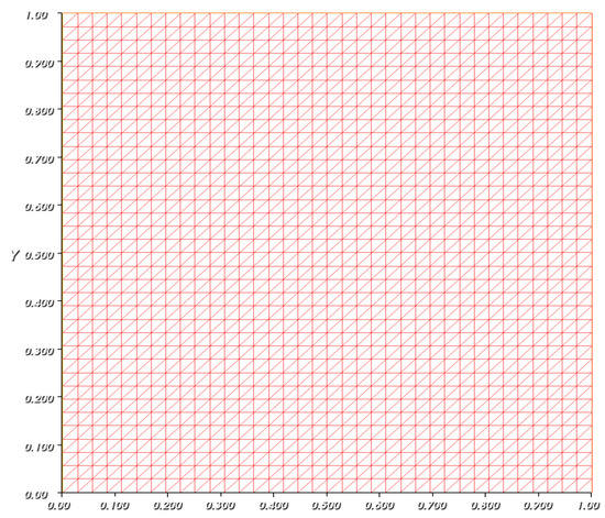
Figure 1. Mesh configuration.

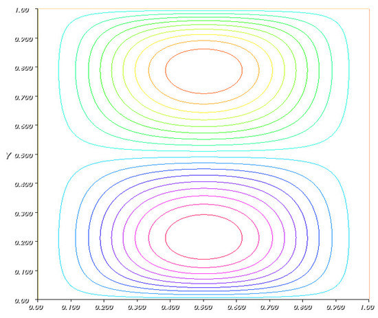
Figure 2. Fluid path or velocity contours.

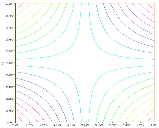
Figure 3. The pressure field lines.

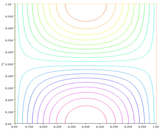
Figure 4. The magnetic field lines.

7. Conclusions

A QLS mixed finite element method (MFE) based on $L^2$-inner product is discussed to solve a coupled and nonlinear incompressible magnetohydrodynamic (MHD) model. The model equations are highly coupled and nonlinear. Some functional spaces were not convenient to transform model equations into the weak formulation due to which the stability issue occurs. Therefore the $L^2$-inner product is utilized as a stabilization technique to circumvent this deficiency. First, we utilized the Oseen-type technique for the conversion of nonlinearity into linearity. Secondly, a direct iteration technique is applied to overcome the nonlinearities and obtained a theoretical convergence rate for the general initial guesswork. Theoretical results show that only a single parameter with a single initial guess is sufficient to establish the well-posedness of the solution.

References

- Alfvén, H. Existence of electromagnetic-hydrodynamic waves. Nature 1942, 150, 405. [Google Scholar] [CrossRef]
- Mitchell, D.L.; Gubser, D.U. Magnetohydrodynamic ship propulsion with superconducting magnets. J. Supercond. 1988, 1, 349–364. [Google Scholar] [CrossRef]
- Al-Habahbeh, O.; Al-Saqqa, M.; Safi, M.; Khater, T.A. Review of magnetohydrodynamic pump applications. Alex. Eng. J. 2016, 55, 1347–1358. [Google Scholar] [CrossRef]
- Davidson, P.A. Magnetohydrodynamics in material processing. Annu. Rev. Fluid Mech. 1999, 31, 273–300. [Google Scholar] [CrossRef]
- Yuksel, G.; Ingram, R. Numerical Analysis of a Finite Element, Crank-Nicolson Discretization for MHD Flow at Small Magnetic Reynolds Number; Tech. Report; University of Pittsburgh: Pittsburgh, PA, USA, 2011. [Google Scholar]
- Shercliff, J.A. Steady motion of conducting fluids in pipes under transverse magnetic fields. Proc. Camb. Philos. Soc. 1953, 49, 136–144. [Google Scholar] [CrossRef]
- Gerbeau, J.-F.; Bris, C.L.; Lelievre, T. Mathematical Methods for the Magnetohydrodynamics of Liquid Metals, Numerical Mathematics and Scientific Computation; Oxford University Press: New York, NY, USA, 2006. [Google Scholar]
- Barleon, L.; Casal, V.; Lenhart, L. MHD flow in liquid-metal-cooled blankets. Fusion Eng. Des. 1991, 14, 401–412. [Google Scholar] [CrossRef]
- Davidson, P.A. An Introduction to Magnetohydrodynamics; Cambridge Texts in Applied Mathematics; Cambridge University Press: Cambridge, UK, 2001. [Google Scholar]
- Roberts, P.H. An Introduction to Magnetohydrodynamics; Elsevier: Alpharetta, GA, USA, 1967. [Google Scholar]
- Codina, R.; Hernadez-Silva, N. Stabilized finite element approximation of the stationary magneto-hydrodynamics equations. Comput. Mech. 2006, 38, 344–355. [Google Scholar] [CrossRef]
- Gunzburger, M.D.; Meir, A.J.; Peterson, J.S. On the existence and uniqueness and finite element approximation of solutions of the equations of stationary incompressible magnetohydrodynamics. Math. Comput. 1991, 56, 523–563. [Google Scholar] [CrossRef]
- Barbosa, H.; Hughes, T. The finite element method with Lagrange multipliers on the boundary: Circumventing the Babuska-Brezzi condition. Comput. Meth. Appl. Mech. Engrgy 1991, 85, 109–128. [Google Scholar] [CrossRef]
- Greif, C.; Li, D.; Schotzau, D.; Wei, X. A mixed finite element method with exactly divergence-free velocities for incompressible magnetohydrodynamics. Comput. Methods Appl. Mech. Engrgy 2010, 45–48, 2840–2855. [Google Scholar] [CrossRef]
- Hasler, U.; Schneebeli, A.; Schözau, D. Mixed finite element approximation of incompressible MHD problems based on weighted regularization. Appl. Numer. Math. 2004, 51, 19–45. [Google Scholar] [CrossRef]
- Schneebeli, A.; Schötzau, D. Mixed finite elements for incompressible magnetohydrodynamics. C. R. Acad. Sci. Paris Ser. I 2003, 337, 71–74. [Google Scholar] [CrossRef]
- Gerbeau, J.F. A stabilized finite element method for the incompressible magnetohydrodynamic equations. Numer. Math. 2000, 87, 83–111. [Google Scholar] [CrossRef]
- Shi, D.; Yu, Z. Nonconforming mixed finite element methods for stationary in-compressible Magnetohydrodynamics. Int. J. Numer. Anal. Model. 2013, 10, 904–919. [Google Scholar]
- Bochev, P.B.; Gunzburger, M.D. Least-squares method for the velocity pressure-stress formulation of the Stokes equations. Comput. Meth. Appl. Mech. Eng. 1995, 126, 267–287. [Google Scholar] [CrossRef]
- Bramble, J.H.; Pasciark, J.E. Least-squares methods for the Stokes equations based on a discrete minus one inner project. J. Comput. Appl. Math. 1996, 74, 155–173. [Google Scholar] [CrossRef][Green Version]
- Bramble, J.H.; Schatz, A.H. Least-squares methods for 2m-th order elliptic boundary-value problems. Math. Comput. 1971, 25, 1–32. [Google Scholar]
- Chang, C.L.; Jiang, B.N. An error analysis of least-squares finite element method of velocity- pressure- vorticity formulation for the Stokes problem. Comput. Methods Appl. Mech. Eng. 1990, 84, 247–255. [Google Scholar] [CrossRef]
- Yang, D.; Wang, L. Quasi-least-squares finite element method for steady flow and heat transfer with system rotation. Numer. Math. 2006, 104, 377–411. [Google Scholar] [CrossRef]
- Qureshi, I.H.; Nawaz, M.; Rana, S.; Nazir, U.; Chamkha, A.J. Investigation of variable thermo-physical properties of viscoelastic rheology: A Galerkin finite element approach. AIP Adv. 2018, 8, 075027. [Google Scholar] [CrossRef]
- Wang, L.; Pang, S.Y.; Cheng, L. Bifurcation and stability of forced convection in tightly coiled ducts: Stability. Chaos Solitons Fractals 2006, 26, 991–1005. [Google Scholar] [CrossRef]
- Bochev, P.B. Analysis of least-squares finite element method for Navier-Stokes equations. SIAM J. Numer. Anal. 1997, 34, 1817–1844. [Google Scholar] [CrossRef]
- Bochev, P.B. Negative norm least-squares finite element mfethod for velocity vorticity pressure Navier Stokes equations. Numer. Meth. Part. Diff. Eqs. 1999, 15, 237–256. [Google Scholar] [CrossRef]
- Cai, Z.; Lazarov, R.; Manteuffel, T.A.; McCormick, S.F. First-order least squares for second-order partial differential equations: Part I. SIAM J. Numer. Anal. 1994, 6, 1785–1799. [Google Scholar] [CrossRef]
- Chang, C.L.; Yang, S.Y. Analysis of the L2 least-squares finite method for the velocity-vorticity-pressure Stokes equations with velocity boundary conditions. Appl. Math. Comput. 2002, 130, 121–144. [Google Scholar] [CrossRef]
- Hussain, S.; Mahbub, M.A.A.; Nasu, N.J.; Zheng, H. stabilized lowest equal-order mixed finite element method for the oseen viscoelastic fluid flow. Adv. Differ. Eq. 2018, 2018, 461. [Google Scholar] [CrossRef]
- Selmi, M.; Naudakumar, K. Bifurcation study of flow through a rotating curved duet. Phys. Fluids 1999, 11, 2030–2043. [Google Scholar] [CrossRef]
- Codina, R.; Hernadez, N. approximation of the thermally coupled MHD problemusing a stabilized finite element method. J. Comput. Phys. 2010, 230, 1281–1303. [Google Scholar] [CrossRef]
- Schötzau, D. Mixed finite element methods for stationary incompressible magneto-hydrodynamics. Numer. Math. 2004, 96, 771–800. [Google Scholar] [CrossRef]
- Gunzburger, M.D.; Ladyzhenskaya, O.A.; Peterson, J.S. On the global unique solvability of initial-boundary value problems for the coupled modified Navier-Stokes Maxwell equations. J. Math. Fluid Mech. 2004, 6, 462–482. [Google Scholar] [CrossRef]
- Prohl, A. Convergent finite element discretizations of the nonstationary incompressible Magnetohydrodynamics system. Esaim Math. Model. Numer. Anal. 2008, 42, 1065–1087. [Google Scholar] [CrossRef]
- Ladyzhenskaya, O.A.; Solonnikov, V. Solution of Some Nonstationary Magnethydrodynamical Problems for Incompressible Fluid. Trusy Steklov Math. Inst. 1960, 59, 115–173. [Google Scholar]
- Hughes, W.F.; Young, F.J. The Electromagneto-Hydrodynamics of Fluids; Wiley: New York, NY, USA, 1966. [Google Scholar]
- Jackson, J.D. Classical Electrodynamics; Wiley: New York, NY, USA, 1975. [Google Scholar]
- Monk, P. Finite Element Methods for Maxwell’s Equations; Oxford University Press: New York, NY, USA, 2003. [Google Scholar]
- Adams, R.; Fournier, J. Sobolev Spaces. Pure and Applied Mathematics; Elsevier Science: Amsterdam, The Netherlands, 2003. [Google Scholar]
- Adams, R.A. Sobolev Space. Pure and Applied Mathematics; Academic Press: New York, NY, USA, 1975; Volume 65. [Google Scholar]
- Girault, V.; Raviart, P.A. Finite Element Methods for Navier-Stockes Equations, Theory and Algorithms; Springer: Berlin, Germany, 1986. [Google Scholar]
- Chang, C. An Error Analysis of Least Squares Finite Element Method of Velocity-Pressure-Vorticity Formulation for Stokes Problem: Correction; Mathematics Research Report; Department of Mathematics, Cleveland State University: Cleveland, OH, USA, 1995. [Google Scholar]
- Chang, C.; Li, J.; Xiang, X.; Yu, Y.; Ni, W. Least squares finite element method for electromagnetic fields in 2-D. Appl. Math. Comput. 1993, 58, 143–167. [Google Scholar]
- Carey, G.F.; Jiang, B.N. Least-squares finite elements for first-order hyperbolic systems. Int. J. Num. Meth. Eng. 1988, 26, 81–93. [Google Scholar] [CrossRef]
- Hecht, F. FreeFEM++. J. Numer. Math. 2012, 20, 251–265. [Google Scholar] [CrossRef]
- Yang, J.; Mao, S.; He, X.; Yang, X.; He, Y. A diffuse interface model and semi-implicit energy stable fnite element method for two-phase magnetohydrodynamics flows. Comput. Methods Appl. Mech. Eng. 2019, 356, 435–464. [Google Scholar] [CrossRef]
Publisher’s Note: MDPI stays neutral with regard to jurisdictional claims in published maps and institutional affiliations. |
© 2022 by the authors. Licensee MDPI, Basel, Switzerland. This article is an open access article distributed under the terms and conditions of the Creative Commons Attribution (CC BY) license (https://creativecommons.org/licenses/by/4.0/).