Intelligent Wavelet Based Pre-Filtering Method for Ultrasonic Sensor Fusion Inverse Algorithm Performance Optimization

Abstract

Certain obstacle mapping applications require the live evaluation of the measured data to prevent collision with obstacles. The fusion of different or similar sensors usually has a high calculation demand, which increases significantly with the area to be evaluated and the number of sensors. In the present considerations, we propose a wavelet-based adaptive optimization method, which can greatly decrease the number of grid points to be evaluated, and thus the necessary computation time. The basis of the method is to use the fact that the areas to be evaluated mostly face a rather small number of obstacles, which cover a smaller percentage of the whole environment. The first step in a pre-filtering process is the determination of the zones where no obstacles are present. This step can already result in a considerable decrease in the computation time, however with the transformation to polar coordinates, the method will not only be more fitted to the problem to be solved, but the area of the evaluation can also be increased with the same number of grid points. As a last step, we applied wavelet transformation to identify the regions of interest, where the application of a refined raster is necessary, and thus further decreasing the number of grid points where the calculation has to be carried out. We used our previously developed probability-based ultrasonic sensor fusion inverse algorithm to demonstrate the efficiency of the proposed method.

1. Introduction

From navigation to mapping, from target localization to obstacle avoidance, ultrasound sensors are widely used, not only in medicine and industry, but also in everyday life. Ultrasound sensors are usually based on the measurement of the time of flight of a ping signal, but a Doppler effect can also help in detecting movements.

If the time of flight is used, the sensor can get the signal directly from the transmitter (direct measurement), or after one or more reflections (indirect measurement). Direct signal measurements are used in practice if the measured object is not detectable with the indirect method—the material of the object to be detected is an absorber for the ultrasound, but a transmitter can be attached to it as a position marker. The measurement to be made if the reflected echoes from an object are to be evaluated, i.e., the indirect measurement, is used in the case of target localization, area mappings, and collision avoidance. For reliable spatial localization multiple transmitters and/or multiple receivers to be used [1,2], the fusion of the signals from the different sources is essential, as well as costly, especially in the case of a larger number of detectors or transmitters.

There have been studies and development toward economical and reliable multi-transmitter ultrasound mapping [1,2] and localization, however, the price to pay for being economic is usually to treat ghost patterns and apply parallel processing algorithms. One of the main challenges of the multiple transmitters is to separate the signals from various sources. Transmitters tuned to different frequencies can usually be the solution, however, in this case frequency-sensitive receivers or frequency filters are needed. Another solution is using code division multiplexing so that the codes of the signals ensure that the signals from the different sources can be separated.

Using a sensor array made of three transmitters and three receivers made it possible to determine and classify given simple shapes [3,4,5], i.e., corners, planes. In these cases, the simultaneous functioning of the transmitters is also difficult to solve, and the signals have to be coded or be of different frequencies. The individual signals are each processed as digital data as one distance measurement per sensor [6].

Classification and digital mapping are very important in mobile robot solutions [7,8], where often a fusion with an optical system is needed to compensate the disadvantages of the two systems.

With a very complex multi-transceiver array, real 3D mapping is also possible, however, the simultaneous functioning of the transceivers and the digital processing of the signals makes the system very slow and not sufficiently precise [2].

There are many aspects of setups with moving localization and environment detection systems that have already been studied. All of them use similar approaches.

The mobile robot-based mapping of unknown areas with a one-dimensional measurement and the movement of the robot have already been developed [9,10], which work simply and effectively, but the mapping is only finished after the robot has swept through the whole area, which is time-consuming. A simple task of navigation by following a wall is also possible with a short feedback—if the wall is continuous—and thus live mapping can be accomplished [11].

As a next step, if the robot is equipped with multiple ultrasonic sensors, triangulation can give more information [12]. The evaluation is faster, than in the case of the 1D, because the triangulation collects more information than the 1D distance measurement in a cycle of one ping, thus the robot needs to sweep a shorter path. If the sensors can be rotated around an axis, it can give one more dimension and it is possible to make a 3D evaluation [13].

The fusion, together with the movement of the device, can be used not only for mapping but also for obstacle avoidance [14]. With the same solution as for the avoidance—1D measurement—with the movement of the sensors, the fusion can be transformed to mapping as well 2D mapping and 3D mapping [15]; however, all of the above listed solutions have another system that gives additional information, so the fusion was performed not just for the ultrasonic sensors.

For wearable devices such as our localisation aid for visually impaired people [16], the device should be able to handle slow motions. We expect that the usage of only ultrasonic sensors will be sufficient for navigation, however, the calculation time should be decreased. In order to achieve our goal, the calculation should be optimized.

In the following considerations, we analyse multiple methods for reducing the necessary computation for one transmitter—the multiple receivers scenarios in the case of reflected measurements. This article researches the possible optimization of our previously developed fusion algorithm for indirect measurements [16]. Specifically, the runtime and the calculation load as well as the possibility of reducing them was studied. We researched the mathematical correlation between the calculation load and the number of receivers and obstacles to make a prediction for runtime.

This paper is structured as follow: first, in Section 2, the mathematical background of the ultrasonic sensor fusion inverse algorithm is summarized. In Section 3, the simple threshold-based optimization was implemented and then tested in Section 4. A prediction of the runtime is given in Section 5, and based on the results, it was determined when is it more economical to use the pre-filtering. In the next two sections, Section 6 and Section 7, the polar coordinate and wavelet transform-based raster modification were implemented, and it was studied as to how they influenced the number of points to be evaluated. The conclusion is drawn in Section 8.

2. Mathematical Establishment of the Pre-Filter Function

Mathematical Evaluation of the Sensor Data

An ultrasound transmitter–receiver pair measures the time of flight of a short burst of ultrasound signal between two devices. The relation between the time of flight t and the distance s is simply expressed by the velocity of the sound $c_s$ as

$$s=c_s·t.$$

(1)

The ultrasound signal can reach the receiver directly from the transmitter or after one or multiple reflections from various objects in the environment. The reflection usually decreases the signal intensity, as part of the signal is absorbed, and partly transmitted through the obstacle.

If a transmitter sends a ping signal towards the object(s) to be measured, then one sensor can determine the distance of that object, or localize it, if the direction is known. If more sensors are used, the localization requires less conditions, i.e., for two sensors, only the plane of the object needs to be known, while three sensors, theoretically, make its localization in a 3D space possible. However, due to measurement uncertainties and the appearance of ghost objects, usually at least one redundant sensor is used. It is also possible to use multiple transmitters if more precise localization is necessary. We use one transmitter and multiple receivers. Theoretically, the method is three-dimensional, but the numerical demonstrations are carried out in two dimensions.

If there is an object, a point-like obstacle at position $\mathbf{P}=(x,y,z)$ which reflects the signal, then the time of flight is proportional to the length of the path followed by the ultrasound signal from the source to the sensor, i.e., to:

$$\begin{array}{ccc}\hfill s_i& =& \sqrt{{\left(r_{ix}-x\right)}^2+{\left(r_{iy}-y\right)}^2+{\left(r_{iz}-z\right)}^2}+\hfill \\ \hfill & +& \sqrt{{\left(R_x-x\right)}^2+{\left(R_y-y\right)}^2+{\left(R_z-z\right)}^2},\hfill \end{array}$$

(2)

if the position of the ith sensor is ${\mathbf{r}}_{\mathbf{i}}=(r_{ix},r_{iy},r_{iz})$, for $i=1,\dots ,I$ and the position of the transmitter is $\mathbf{R}=(R_x,R_y,R_z)$, which is chosen to be the origin in the following considerations.

Signals are received from all the sensors, each of them providing information about the space around the transmitter–receiver pair in ellipsoid coordinates. In order to determine, whether there is an obstacle at a given domain of the space around the sensors and transmitter, it is more convenient to create a Cartesian coordinate based grid of a given resolution, and calculate the fusion of the signals from all sensors for each of the grid points. If a point of the grid is $(x_a,y_b,z_c)$ then the signal’s travel time–distance at the position corresponding to the index triplet $(a,b,c)$ from sensor i can be determined using the Equation (3):

$$\begin{array}{ccc}\hfill {\mathbf{S}}_{iabc}& =& \sqrt{{\left(r_{ix}-x_a\right)}^2+{\left(r_{iy}-y_b\right)}^2+{\left(r_{iz}-z_c\right)}^2}+\hfill \\ \hfill & +& \sqrt{x_a^2+y_b^2+z_c^2}.\hfill \end{array}$$

(3)

Because of the transmitter being chosen to be in the origin, its coordinates are eliminated from the equation. Here, the indices of the grid coordinate $(x_a,y_b,z_c)$ fulfill the condition $a=1,\dots ,A$, $b=1,\dots ,B$, and $c=1,\dots ,C$, where the A, B and C are the indices of the coordinate of the last grid point. This generates a four-dimensional grid matrix:

$$\mathbf{S}=\left[\begin{array}{cccc}{\mathbf{S}}_{\mathbf{p}11}& {\mathbf{S}}_{\mathbf{p}21}& \dots & {\mathbf{S}}_{\mathbf{p}A1}\\ {\mathbf{S}}_{\mathbf{p}12}& {\mathbf{S}}_{\mathbf{p}22}& \dots & {\mathbf{S}}_{\mathbf{p}A2}\\ ⋮& ⋮& & ⋮\\ {\mathbf{S}}_{\mathbf{p}1B}& {\mathbf{S}}_{\mathbf{p}2B}& \dots & {\mathbf{S}}_{\mathbf{p}AB}\end{array}\right],$$

(4)

where the shorthand notation:

$${\mathbf{S}}_{\mathbf{p}ab}=\left[\begin{array}{cccc}{S}_{1ab1}& S_{1ab2}& \dots & S_{1abC}\\ S_{2ab1}& S_{2ab2}& \dots & S_{2abC}\\ ⋮& ⋮& & ⋮\\ S_{Iab1}& S_{Iab2}& \dots & S_{IabC}\end{array}\right]$$

(5)

was used for the sub-matrices.

Using the 4D distance matrix (4), the data measured by the individual sensors can be evaluated in the following way. First, for the ith sensor, for all the locations on the grid $(x_a,y_b,z_c)$, the approximation of the measured signal intensity can be calculated by interpolation. This means, that if we have a measured point at each integer $a,b,c$, then the value corresponding to the distance ${\mathbf{S}}_{iabc}$ is:

$$\begin{array}{ccc}\hfill \mathbf{A}\left({\mathbf{S}}_{iabc}\right)& =& \mathbf{A}\left(⌊{\mathbf{S}}_{iabc}⌋\right)+\frac{{\mathbf{S}}_{iabc}-⌊{\mathbf{S}}_{iabc}⌋}{⌈{\mathbf{S}}_{iabc}⌉-⌊{\mathbf{S}}_{iabc}⌋}\times \hfill \\ \hfill & \times & \left(\mathbf{A}\left(⌈{\mathbf{S}}_{iabc}⌉\right)-\mathbf{A}\left(⌊{\mathbf{S}}_{iabc}⌋\right)\right).\hfill \end{array}$$

(6)

As ${\mathbf{S}}_{iabc}$ can be non-integer, and the measurement result of each sensor is available only in integer locations, an interpolation is needed. By the operations $\lfloor •\rfloor$ and $\lceil •\rceil$ i.e., the floor and the ceiling operators, the two neighboring points can be determined, and with a linear interpolation, the value of $\mathbf{A}\left({\mathbf{S}}_{iabc}\right)$ can be approximated. Combining the signals of the different sensors in this case means that the values $\mathbf{A}\left({\mathbf{S}}_{iabc}\right)$ are to be fused along the dimension i. The fusing algorithm can be a simple multiplication of the signal values corresponding to each grid point, however, this method can be disturbed by different sensor types and sensitivities (practically, because of the tolerances in the production of the circuits and the sensors, there are no identically sensitive sensor modules, even from the same manufacturer). To be able to use different types of sensors simultaneously, the simplest way to overcome sensitivity differences is to re-normalize the sensor intensity by its maximum sensed value according to:

$${\mathbf{A}}^{*}\left[{\mathbf{S}}_{iabc}\right]=\frac{\mathbf{A}\left[{\mathbf{S}}_{iabc}\right]}{A_{max}}.$$

(7)

This step makes the method able to use sensors with a different sensitivity level, angle, and amplification.

Thus, the fusion for the sensors gives a probability distribution matrix according to the formula:

$$\mathbf{P}\left[a,b,c\right]=\prod _{i=0}^I{\mathbf{A}}^{*}\left[{\mathbf{S}}_{iabc}\right].$$

(8)

In the case of fusion, a sensor system can be fused with other sensors, to exploit the advantages and to suppress the disadvantages of the other systems. The movement of the system can also be a factor that influences the fusion, e.g., when a mobile robot is mapping its environment, then the position, orientation or the relative dislocation must be included in the algorithm.

The key factor for a wearable localization device is the fast processing of the data, as faster processing allows more time for the user to react and avoid a collision.

3. Calculation Optimization of the Algorithm

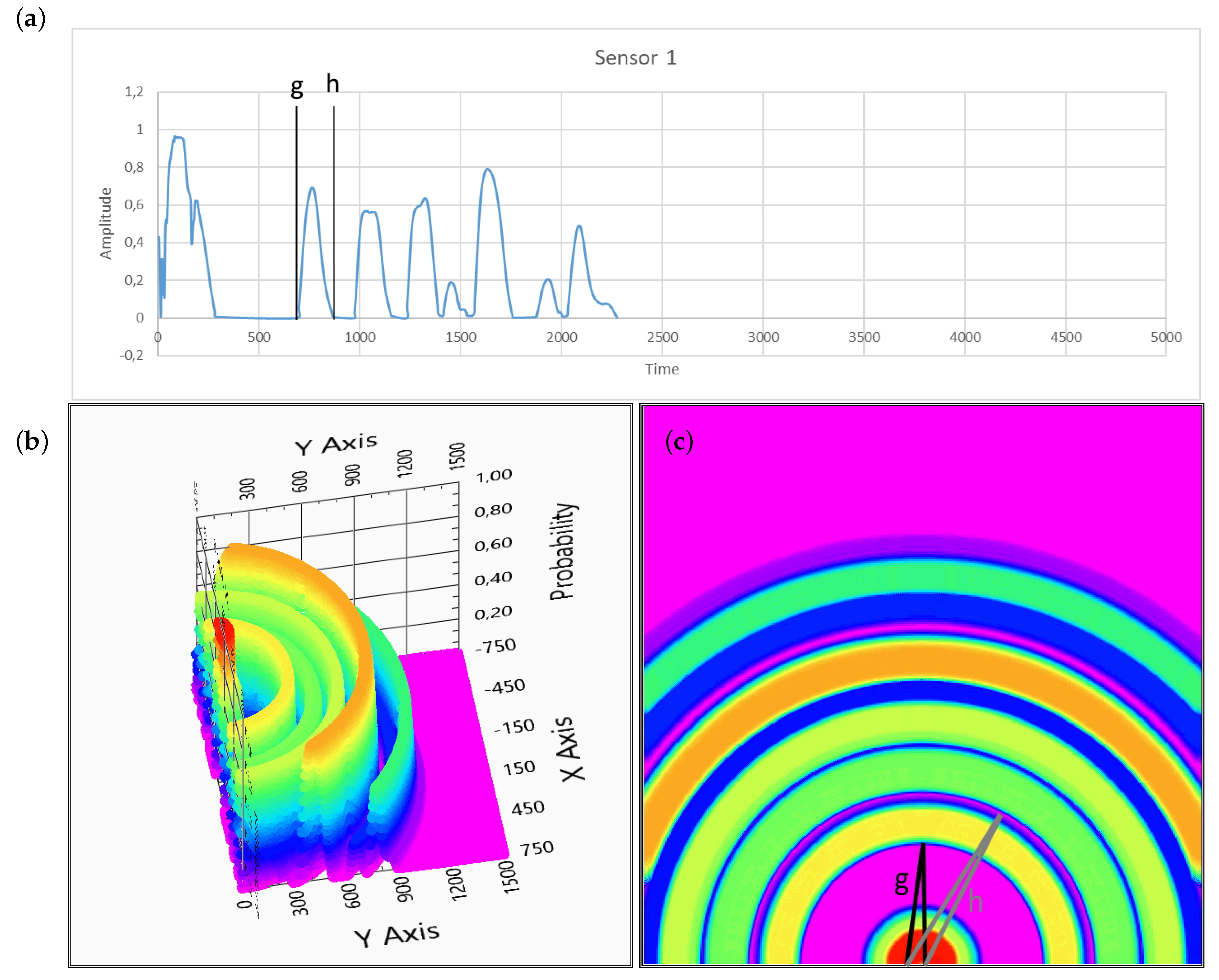
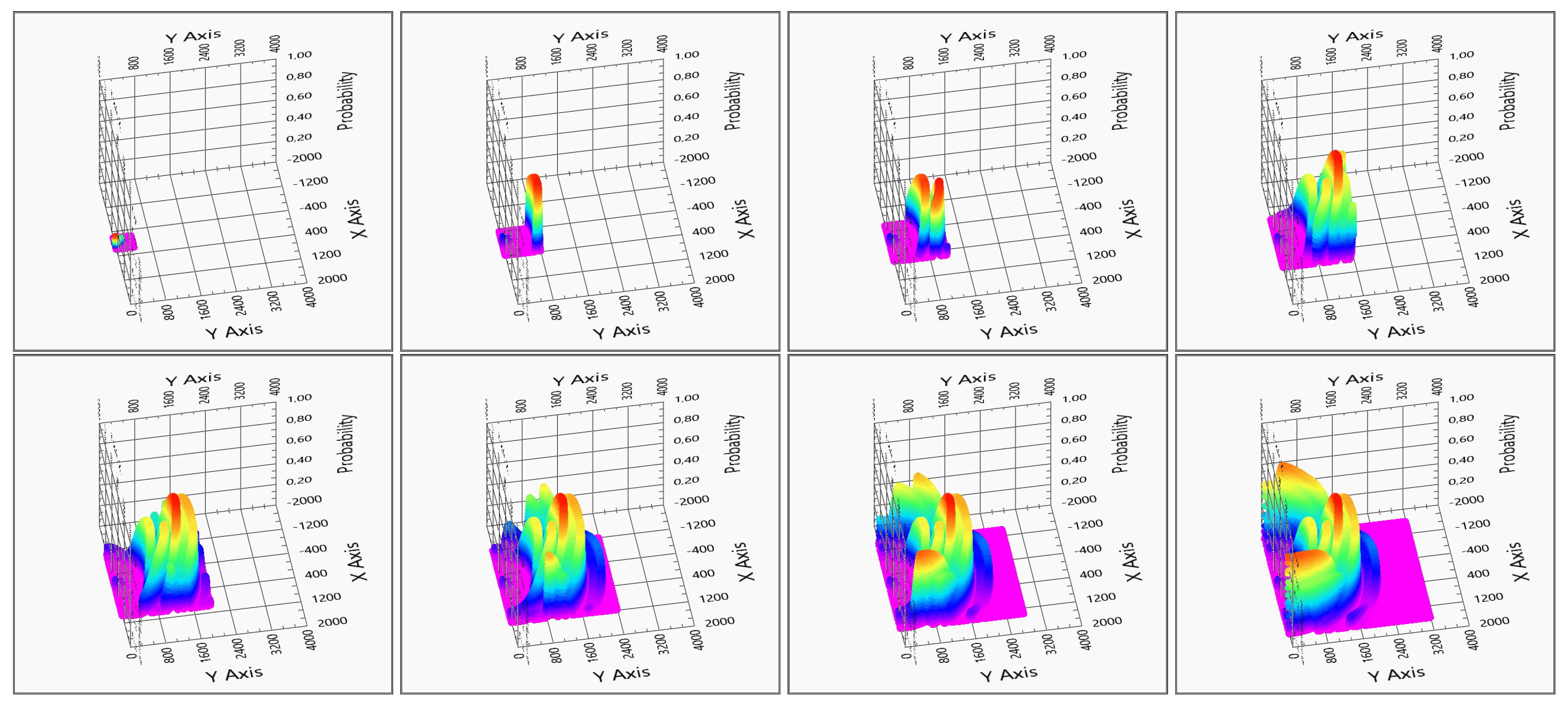
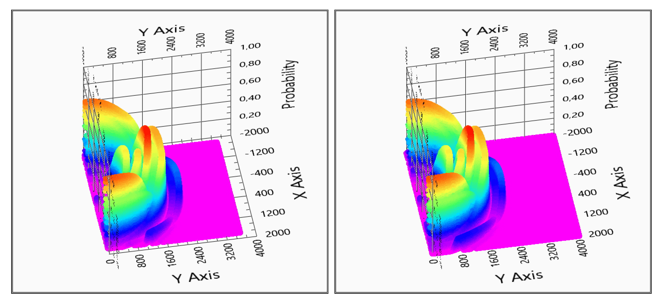
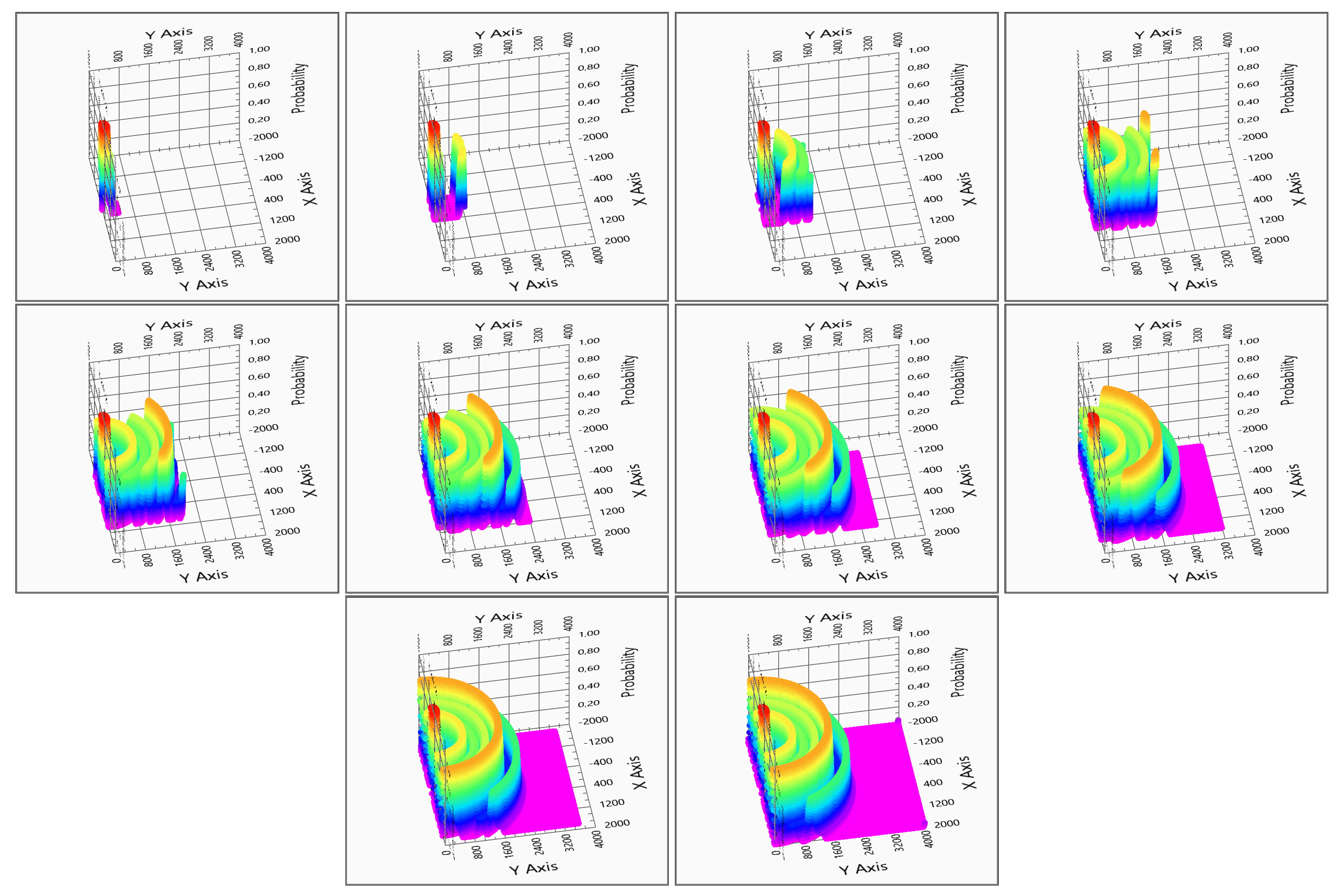
3.1. Calculation of the Possibility for a Space–Point Array

To run the calculation for a part of the space rather than just for one point, we have to go back to the root model with the reference system, i.e., to the usage of the ellipsoids coordinate system and not the Cartesian system. To determine the possibility of an obstacle for a given part of the ellipsoids from each sensor, the calculation has to be the following. If Figure 1 represents the envelope of the signal $A\left(l\right)$ of a sensor, then the possibility ${\mathbf{P}}_{gh}$ of an obstacle being present between the ellipsoid shells is:

$${\mathbf{P}}_{gh}=\frac{{\int }_g^{h}A\left(l\right)dl}{(h-g)·A_{max}}.$$

(9)

Here, l is the distance calculated from the time parameter of the received signal similarly to Equation (1), and h and g give the start and end of the index of the ellipsoid segment to be evaluated, i.e., the distances that are calculated from the starting and the ending time of the non-zero part of the received signals, as marked in the first and third subplots of Figure 1. Based on this idea, the signal can be split into intervals where the signal is above a given level (i.e., something is in the sensing area), and to zones where the signal is low (i.e., there is nothing in the sensing area). Figure 1 shows the variables g and h of Equations (9)–(12).

In the case of a discrete measurement, the algorithm uses a sum not an integral:

$${\mathbf{P}}_{gh}=\frac{{\sum }_{l=g}^{h}A\left(l\right)}{(h-g)·A_{max}},$$

(10)

Further calculations for multiple sensors can be a bit complex, but solution can be given as intersections of segments of the ellipsoids from the equation, if the calculation runs for each sensor, but with defined starting and ending indices:

$${\mathbf{P}}_{ghi}=\frac{{\sum }_{l=g}^h{A}_i\left(l\right)}{(h-g)·A_{max}}$$

(11)

$$\begin{array}{ccc}\hfill {\mathbf{P}}_{Slice}& =& \frac{{\sum }_{l=g}^h{A}_1\left(l\right)}{(h-g)·A_{max}}·\frac{{\sum }_{l=i}^j{A}_2\left(l\right)}{(j-i)·A_{max}}·\frac{{\sum }_{l=k}^m{A}_3\left(l\right)}{(m-k)·A_{max}}·\dots \hfill \\ & =& P_{gh1}·P_{ij2}·P_{km3}·\dots ·P_{“start”“stop”“sensorindex”}\hfill \end{array}$$

(12)

3.2. Intelligent Searching for Low Amplitude Domains to Decrease the Calculation Load

To decrease the calculation time, it is advisable to skip some unnecessary calculations. There are more solutions to optimize, and there is no need to calculate every point. To achieve the same result as the old algorithm, where every point was evaluated, we should make some automatic simplification, and for that, the following rules have to be followed:

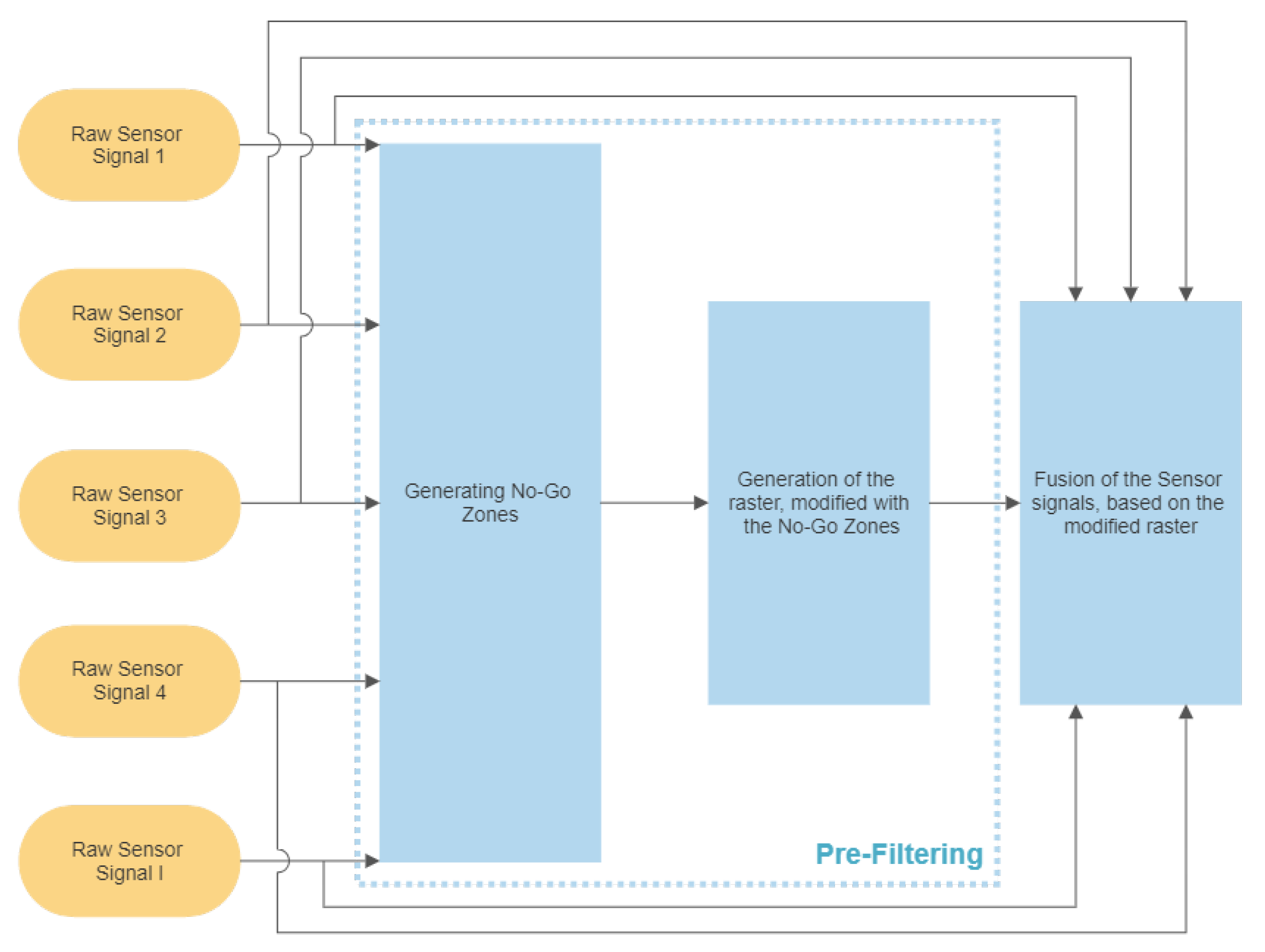
• If in a given position one sensor does not detect (i.e., ${\mathbf{A}}^{*}\left[{\mathbf{S}}_{iabc}\right]=0$), then the possibility is 0;
• Check and store the lower and upper limits of 0 possibility domains for each sensor;
• Create no-go zones from this 0 possibility domain for each sensor;
• In no-go zones, the calculation of the possibility (8) is not carried out, and it has to be 0.

With this automatic intelligent pre-filtering, the algorithm can save time.

4. Comparison with and without the Pre-Filtering Regarding the Evaluated Area Size and the Number of the Sensors

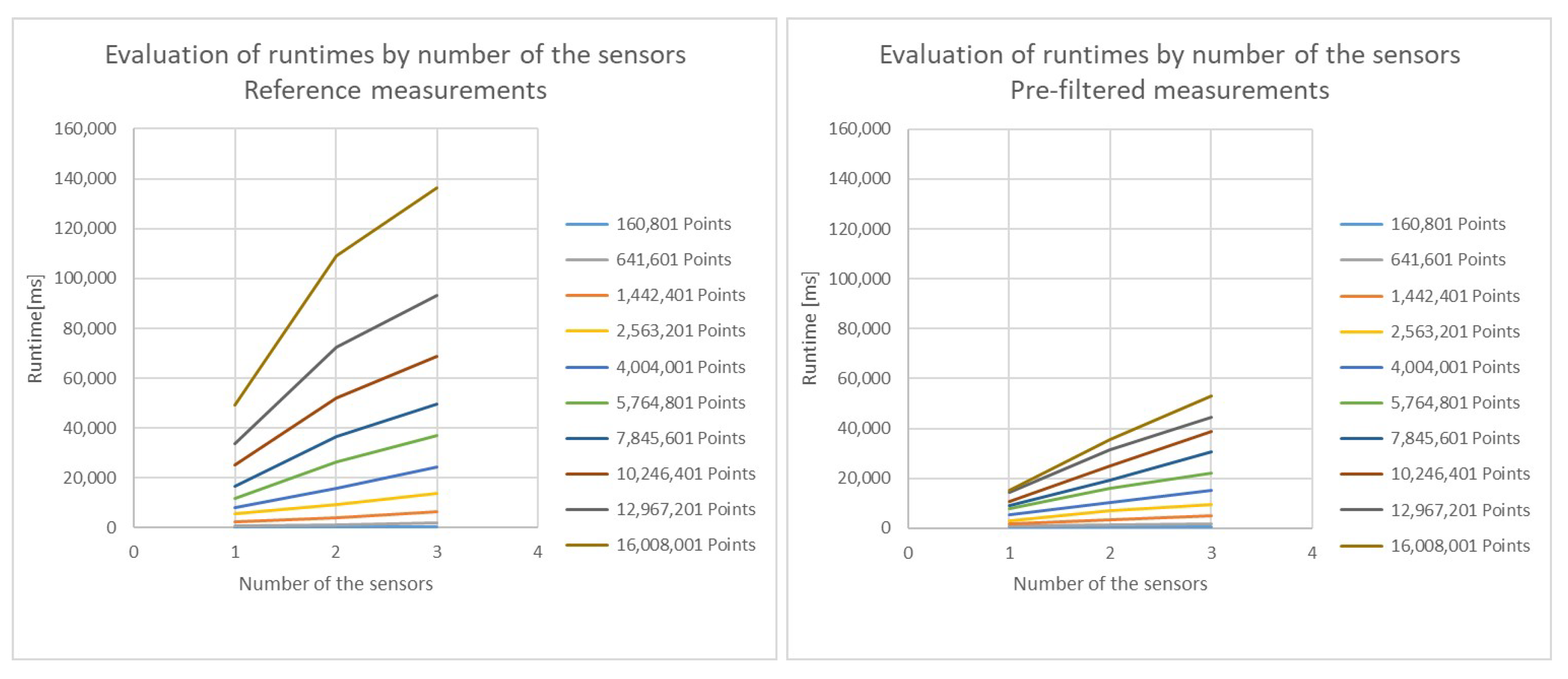
4.1. Reference Runs with Different Number of Points to Be Evaluated

In order to study the efficiency of the algorithms, a reference run was needed with the original algorithm, and during the runs, the main running parameters were recorded.

The measurement was implemented in an environment where the occupation ratio and the number of active sensors could be varied the following way. We used complex data from a previous three sensor measurement [16] in a large area, with various obstacles present, each located at different distances from the sensors. The top view of the measurement setup is shown in Figure 2. During the tests, different sized parts of the original measurements were evaluated, thus achieving a different number of evaluated points and different occupation ratios of the area. The results of these calculations can be seen in Figure 3. During the calculation, the runtime and the number of the cycles of each program blocks were measured, as is visible in the

Table A1. Reference measurement results without pre-filtering with 3 receivers.

Evaluated Points	Amplitude Approximation (# of Runs)	Amplitude Approximation (ms)
160,801	482,403	437.5
641,601	1,924,803	2156.2
1,442,401	4,327,203	6500.0
2,563,201	7,689,603	13,812.5
4,004,001	12,012,003	24,218.8
5,764,801	17,294,403	37,140.6
7,845,601	23,536,803	49,843.8
10,246,401	30,739,203	68,703.1
12,967,201	38,901,603	93,375.0
16,008,001	48,024,003	136,578.1

. We also used the following conditions:

• The number of evaluated points was between 160,801 and 16,008,001;
• The number of sensors were 3;
• The occupation of the area was between 24.1% and 44.1%.

4.2. Pre-Filtered Runs with Different Number of Evaluated Points

After the evaluation of the test runs of the pre-filtering, the results show us that in most cases, the algorithm has positive influence on the runtime, but not with every boundary condition. The reference runtime measurement and the pre-filtered runtime plots are visible on the Figure 4. In addition, the plots the pre-filtered runs were recorded with the same method as the reference. The reference measurement results are shown in Table A1, while the pre-filtered ones are in

Table A2. Measurement results with pre-filtering and 3 receivers.

Evaluated Points	Amplitude Approx. (# of Runs)	Amplitude Approx. (ms)	Pre-Filter (ms)	Pre-Filter (# of Runs)	Array Integral (ms)	Array Integral (# of Runs)	Occupation (%)	SUM (ms)
160,801	150,150	140.6	390.6	482,403	0	3	31.1	531.2
641,601	354,267	343.8	1453.1	1,924,803	0	3	18.4	1796.9
1,442,401	1,271,811	1453.1	3468.8	4,327,203	0	3	29.4	4921.9
2,563,201	3,148,599	3578.1	5890.6	7,689,603	0	3	40.9	9468.7
4,004,001	5,302,455	6375	8859.4	12,012,003	0	3	44.1	15,234.4
5,764,801	7,515,594	9437.5	12,468.8	17,294,403	0	3	43.5	21,906.3
7,845,601	8,800,671	10,625	20,171.9	23,536,803	0	3	37.4	30,796.9
10,246,401	10,152,120	12,187.5	26,500.0	30,739,203	0	3	33.0	38,687.5
12,967,201	11,125,824	14,406.2	30,187.5	38,901,603	0	3	28.6	44,593.7
16,008,001	11,670,015	15,296.9	37,875.0	48,024,003	0	3	24.3	53,171.9

. The structure of the method is shown in Figure 5:

The decrease in the runtime between the reference and the pre-filtered measurement in the best case was 39%, and it is also statable that with the increase in the number of evaluated points, the decrease in runtime is bigger, in the case of a similar or lower occupation ratio of the space.

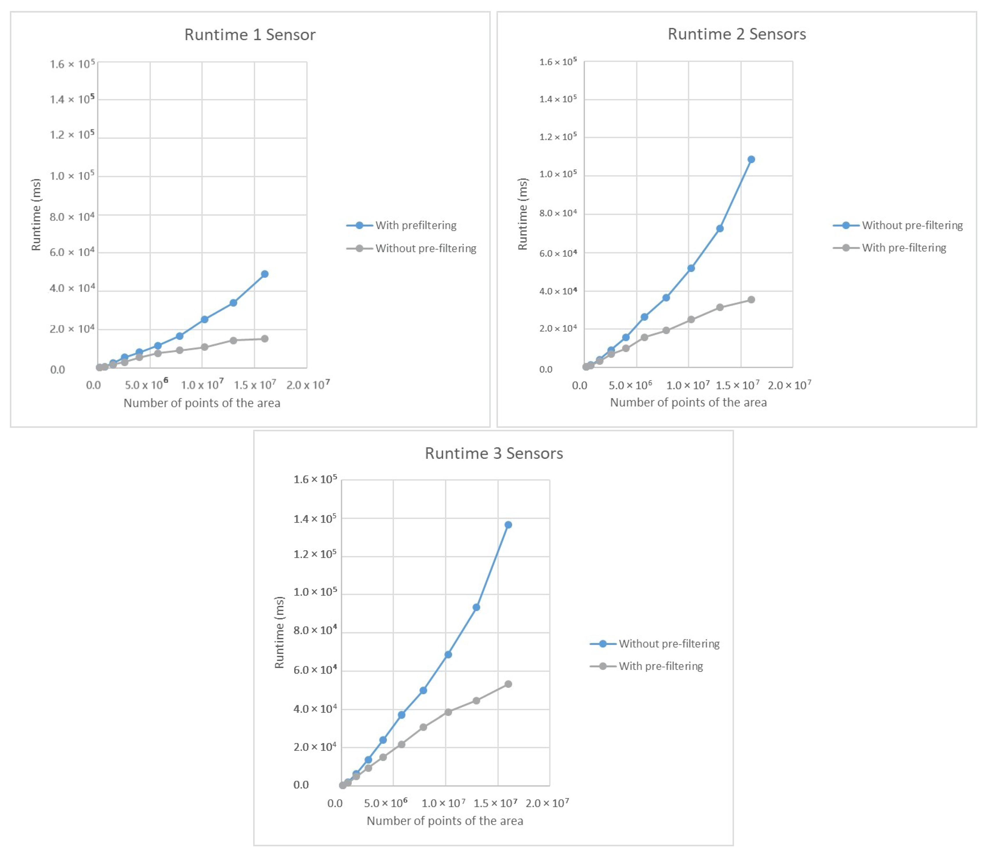
4.3. Changes of the Runtime Based on the Number of the Sensors

Figure 3, Figure 6 and Figure 7 all belong to both the reference run and the pre-filtered measurements, though the calculated probability matrix does not change. It is visible in Figure 3, Figure 6 and Figure 7 that the number of the sensors has a big influence on the details of the evaluated area, and the ghost objects disappear as the number of used receivers increases. In addition to the influence of the evaluation precision, the runtime was also increased together with the number of sensors. In the case of the reference measurement—without pre-filtering—the runtime is not linearly influenced by the change in the number of sensors, i.e., the cost of the additional sensor is less for the third one than for the second.

The connection between the sensor numbers and the runtime in the case of the pre-filtered measurement was not only influenced by the number of the senors, but also by the occupation ratio of the area. For amplitude approximation (6), the used number of sensors roughly linearly influences the runtime.

The decrease in the runtime between the reference measurement and the pre-filtered one was the best for one receiver, shown in Figure 8. In the best case, the runtime with the pre-filtering could be decreased to 31% of the reference measurement for one receiver, and for two and three receivers these ratios were 32% and 39%, respectively. If the decrease is shown in absolute runtime difference, the result is 33,843.7 ms with one receiver, 73,484.4 ms with two and 83,406.2 ms with three. The detailed numerical results are shown in the Appendix A. The reference measurement results listed in Table A1,

Table A3. Measurement results without pre-filtering with 2 receivers.

Evaluated Points	Amplitude Approximation (# of Runs)	Amplitude Approximation (ms)
160,801	321,602	296.9
641,601	1,283,202	1265.6
1,442,401	2,884,802	4078.1
2,563,201	5,126,402	9234.4
4,004,001	8,008,002	15,937.5
5,764,801	11,529,602	26,578.1
7,845,601	15,691,202	36,578.1
10,246,401	20,492,802	52,015.6
12,967,201	25,934,402	72,500.0
16,008,001	32,016,002	108,921.9

and

Table A5. Measurement results without pre-filtering with 1 receiver.

Evaluated Points	Amplitude Approximation (# of Runs)	Amplitude Approximation (ms)
160,801	160,801	140.6
641,601	641,601	734.4
1,442,401	1,442,401	2593.8
2,563,201	2,563,201	5562.5
4,004,001	4,004,001	8156.2
5,764,801	5,764,801	11,750.0
7,845,601	7,845,601	16,750.0
10,246,401	10,246,401	25,359.4
12,967,201	12,967,201	33,906.2
16,008,001	16,008,001	49,062.5

and the pre-filtered ones are given in Table A2,

Table A4. Measurement results with pre-filtering with 2 receivers.

Evaluated Points	Amplitude Approx. (# of Runs)	Amplitude Approx. (ms)	Pre-Filter (ms)	Pre-Filter (# of Runs)	Array Integral (ms)	Array Integral (# of Runs)	Occupation (%)	SUM (ms)
160,801	100,100	93.8	250.0	321,602	0	2	31	343.8
641,601	237,100	265.6	859.4	1,283,202	0	2	18	1125.0
1,442,401	862,106	984.4	2328.1	2,884,802	0	2	30	3312.5
2,563,201	2,260,698	2796.9	4156.2	5,126,402	0	2	44	6953.1
4,004,001	4,013,918	4593.8	5500.0	8,008,002	0	2	50	10,093.8
5,764,801	5,705,024	6171.9	9703.1	11,529,602	0	2	49	15,875.0
7,845,601	6,798,012	7453.1	11,890.6	15,691,202	0	2	43	19,343.7
10,246,401	7,858,932	8921.9	16,078.1	20,492,802	0	2	38	25,000.0
12,967,201	8,665,870	9437.5	21,937.5	25,934,402	0	2	33	31,375.0
16,008,001	9,233,954	10,750.0	24,687.5	32,016,002	0	2	29	35,437.5

and

Table A6. Measurement results with pre-filtering with 1 receiver.

Evaluated Points	Amplitude Approx. (# of Runs)	Amplitude Approx. (ms)	Pre-Filter (ms)	Pre-Filter (# of Runs)	Array Integral (ms)	Array Integral (# of Runs)	Occupation (%)	SUM (ms)
160,801	114,302	203.1	125.0	160,801	0	1	71	328.1
641,601	231,110	281.2	437.5	641,601	0	1	36	718.7
1,442,401	653,861	640.6	984.4	1,442,401	0	1	45	1625.0
2,563,201	1,490,006	1390.6	1609.4	2,563,201	0	1	58	3000.0
4,004,001	2,498,445	2593.8	2875	4,004,001	0	1	62	5468.8
5,764,801	3,873,273	3656.2	4046.9	5,764,801	0	1	67	7703.1
7,845,601	4,541,136	4015.6	5125.0	7,845,601	0	1	58	9140.6
10,246,401	5,179,844	4515.6	6359.4	10,246,401	0	1	51	10,875.0
12,967,201	5,743,590	5328.1	8984.8	12,967,201	0	1	44	14,312.9
16,008,001	6,180,412	5609.4	9609.4	16,008,001	0	1	39	15,218.8

.

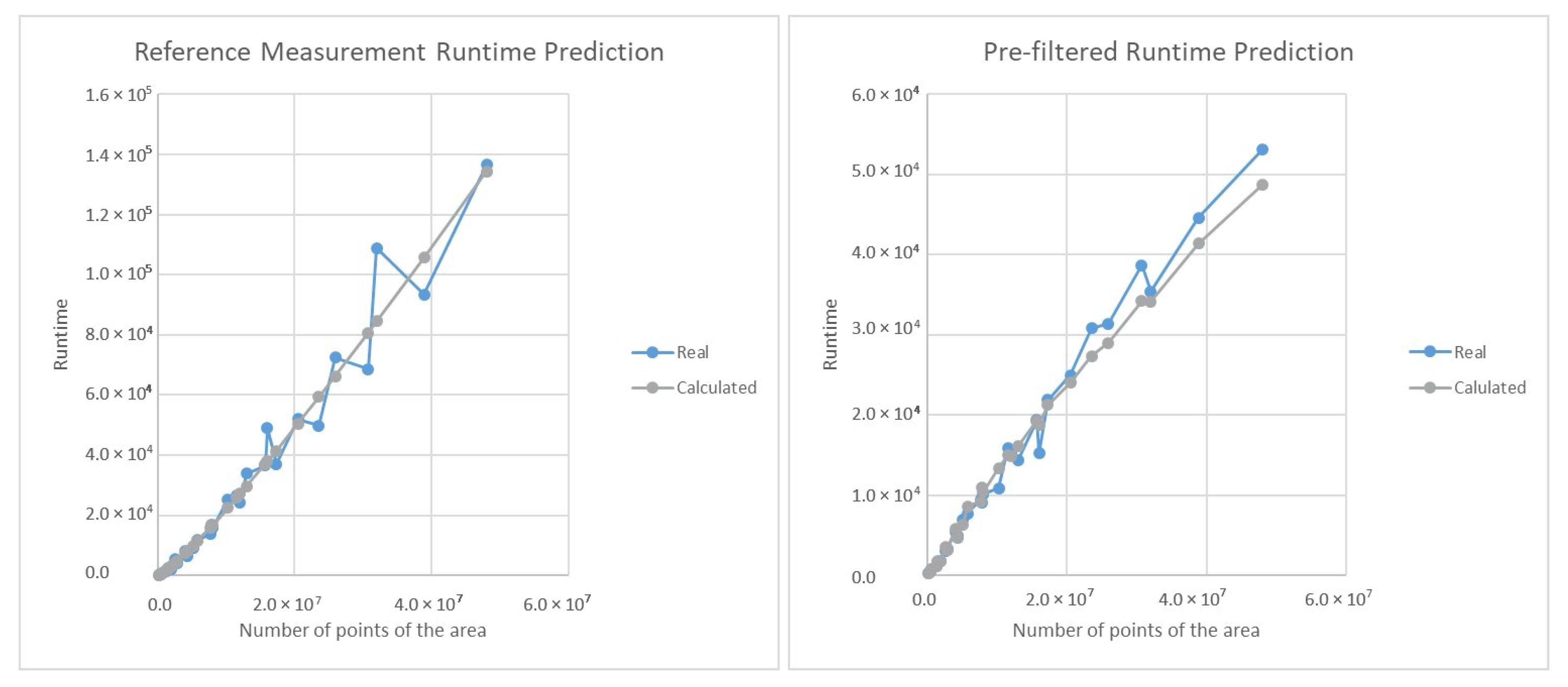
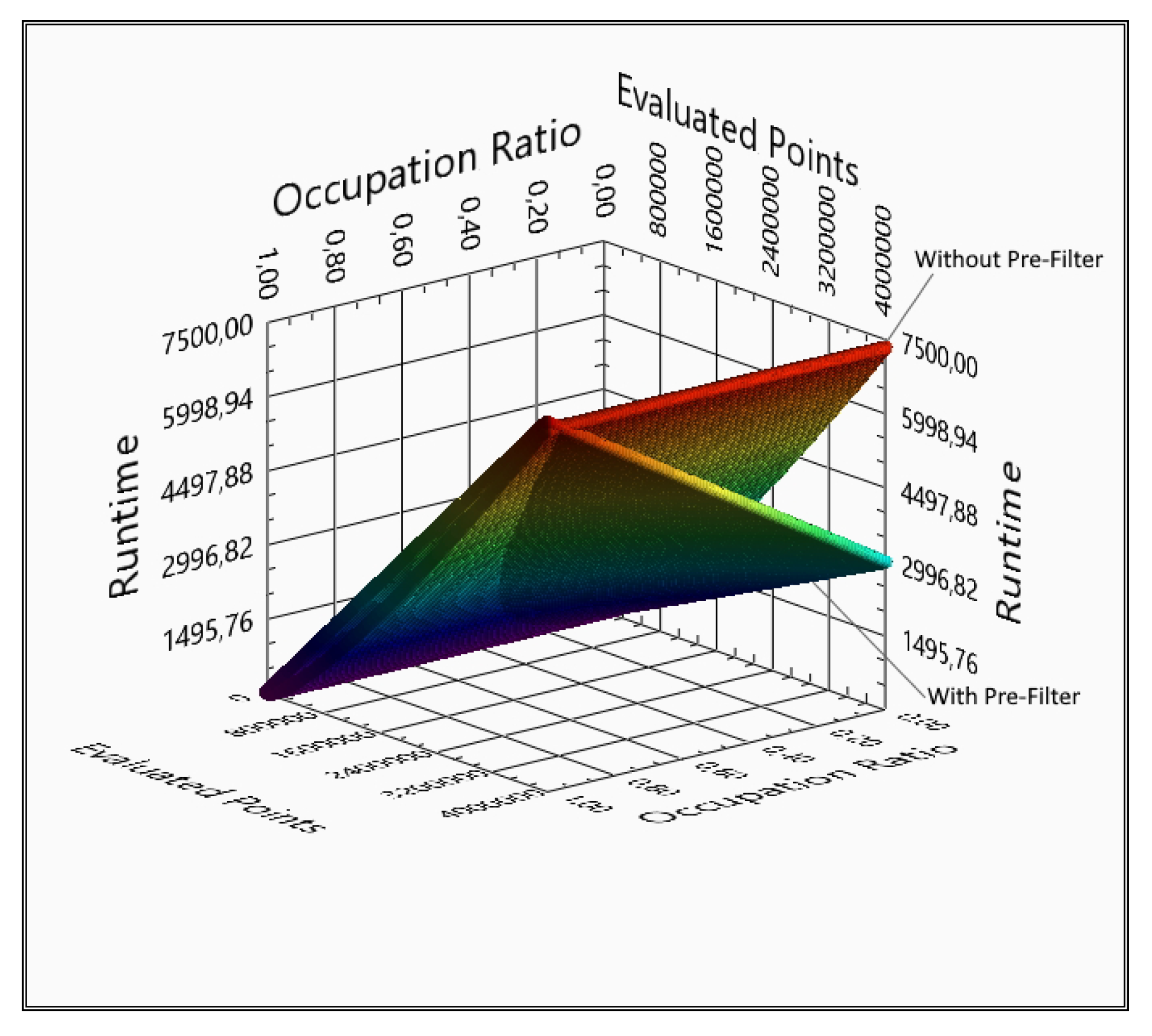
5. Prediction of the Runtime

The first basic assumption is that we can forecast the runtime $t_{ref}$ (13) of the algorithm without pre-filtering from any consideration of the previous sections (Section 3). From the mathematical deduction, the runtime depends only on the number of the evaluated points n. According to the practical measurements, it is visible that the correlation is not simple proportion: it has a logarithmic component as well. Depending on the technical background—the processor used, development environment, etc.—we can describe the system with two constants $C_1$ and $C_2$, as shown below:

$$t_{ref}=n·(C_1·ln(n-C_2)).$$

(13)

The constants $C_1$ and $C_2$ are different for each device that performs the calculation which means that for each individual device, test measurements have to be carried out and these parameters have to be fitted to these results. In the pre-filtered case, the forecasted runtime $t_{pre}$ depends not only on the number of evaluated points n, but there is an impact of the occupation ratio r, and the average pre-filter runtime $t_{filt}$, and the average searching runtime $t_s$, thus, the following equation is given:

$$t_{pre}=n·t_{filt}+n·r·t_s.$$

(14)

Comparing the calculation of the prediction and the real measurement, Figure 9 shows that the results match adequately.

From the prediction and mathematical equations, based on the boundary conditions—evaluated point, occupation ratio—it can be predicted whether the pre-filtering algorithm provides us with any benefit, and how great the runtime difference is.

According to the plot which is visible in Figure 10, the domains optimal for each of the methods, and based on them, it can be determined when the pre-filtering has benefits.

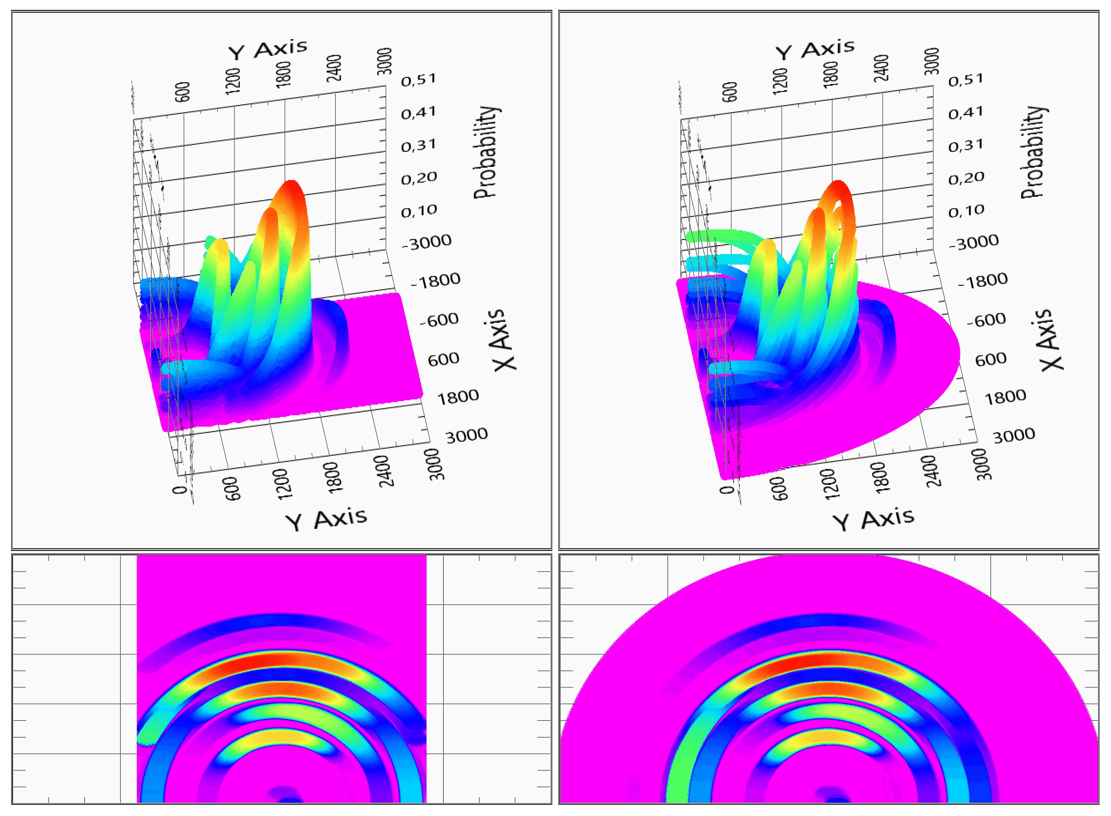
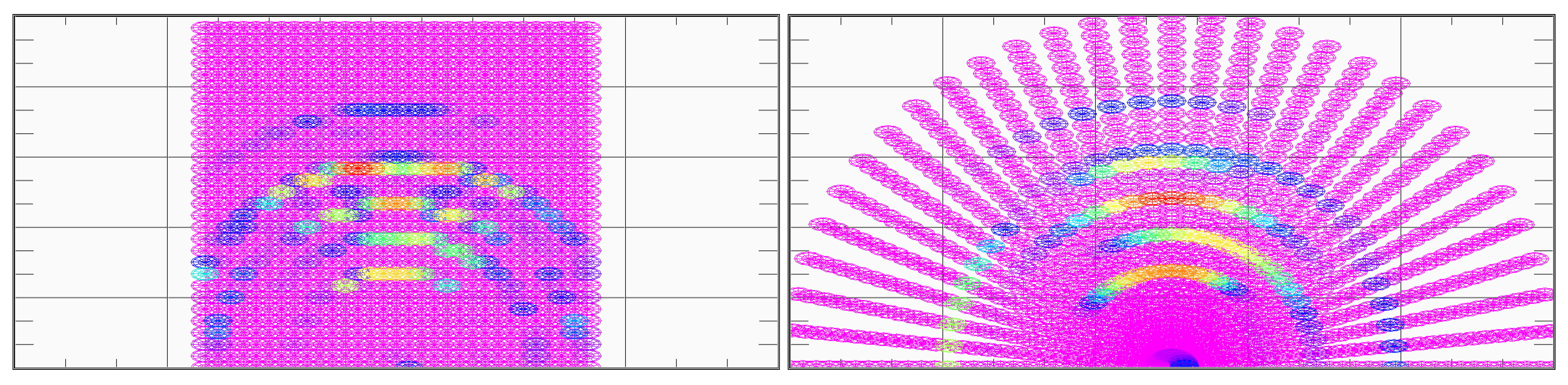
6. Raster Modification with Prioritized Direction

The base of the algorithm is a Cartesian coordinate system, but for a better efficiency, by changing to the polar coordinate system, the result can bring better information with the same runtime, or the same level of information with a lower runtime. The polar coordinate system may also be a better match for human hearing, is directional and distance-based and not Cartesian raster-based. There were measurements for determining the directional resolution of the human hearing both for people with healthy vision and for visually impaired. It was proven that the resolution and the precision were not significantly different for these two groups [17].

In Figure 11, it is visible that the polar coordinate system gives a larger area coverage $A_{pol}$ (15) than the Cartesian one $A_{cart}$ (16), which can be calculated from the radius r of the evaluated area as shown in Equation (15), in the case of the same numbers of evaluated points. Based on the assumptions that the Cartesian evaluation area is a square—i.e., the width x and the depth y are equal—and the radius of the polar coordinate system is equal to the depth of the evaluation area of the Cartesian one, then the area difference can be calculated as it is shown in Equation (17):

$$A_{pol}=\frac{\pi ·r^2}{2},$$

(15)

$$A_{cart}=x·y,$$

(16)

$$A_{pol}=A_{cart}\frac{\pi }{2}.$$

(17)

The area increase of $57\%$—based on (17)—with the same number of evaluated points evidently gives less measurement density in some areas as shown in Figure 12. In order to make the difference between the evaluated point positions visible, the number of the evaluated points were decreased by 100 times in the Figure 12. Despite the fact that the resolution is not constant, in the case of the polar coordinate system, the top view provides better visibility of the results, because of the elipticity of the mathematic correlations.

The raster modification makes it possible to have a non-linearly distributed angle raster. Based on this, the algorithm can focus on the angle of the given direction shown in Figure 13. Of course, it is possible to introduce and handle not only one, but multiple directions of interest.

7. Raster Modification with Prioritized Places

It is visible that with pre-selected priorities, the algorithm can decrease the runtime. The most important possibility for preselecting directions would be previous knowledge of the places of the locations of detectable objects. In this case the raster resolution could be high in needed places and could be lower elsewhere. For the detection of the positions and the sizes of the objects, precalculation is needed from the raw sensor signals.

Previously, some articles have already calculated the positions of the measured objects from multiple sensor measurements, but instead of calculating the absolute position of the objects, the angles were determined. This also gives the required information, even though the sensors can not distinguish from which object the signal is emitted if multiple objects are measured [18,19,20]. Therefore, another correlation needs to be used.

For a receiver and transmitter pair, their corresponding time of flight determines an ellipse in 2D or ellipsoid in 3D where the obstacle can be located. Part of the system—some of the receivers and the transmitter—can be modeled as two ellipses in 2D or three ellipsoids in 3D which intersect each other. This intersection point gives the position of an obstacle. In the case of the 2D model with the transmitter being in the origin, and the shifts of the receiver positions $x_1$, $x_2$ on the axis and with $a_1$, $a_2$ semi major $a_1$, $a_2$ and semi minor axes $b_1$, $b_2$ the solution of the following equation system (18) gives the intersection point coordinates x, y:

$$\begin{array}{ccc}\hfill \frac{{\left(x-x_1\right)}^2}{a_1^2}+\frac{y^2}{b_1^2}& =& 1,\hfill \\ \hfill \frac{{\left(x-x_2\right)}^2}{a_2^2}+\frac{y^2}{b_2^2}& =& 1.\hfill \end{array}$$

(18)

The measured distances $l_1$, $l_2$ have a direct effect on the semi major $a_1$, $a_2$ and semi minor axes $b_1$, $b_2$, defined by Equation (19):

$$\begin{array}{ccc}\hfill a_1& =& \frac{l_1}{2}\hfill \\ \hfill a_2& =& \frac{l_2}{2}\hfill \\ \hfill b_1& =& \sqrt{a_1^2-x_1^2}\hfill \\ \hfill b_2& =& \sqrt{a_2^2-x_2^2}.\hfill \end{array}$$

(19)

For better demonstration, the following calculation will be performed in 2D. From two given sensors the measured objects’ positions can be calculated, from the position of the sensors $x_1$, $x_2$ and the measured distances $l_1,l_2$ according to the following Equation (20), which are the consequences of Equations (18) and (19):

$$\begin{array}{ccc}\hfill x& =& \frac{\frac{l_1^2\left(\frac{l_2^2}{4}-x_2^2\right)x_2}{2}-\frac{l_2^2\left(\frac{l_1^2}{4}-x_1^2\right)x_1}{2}}{\frac{l_1^2\left(\frac{l_2^2}{4}-x_2^2\right)}{2}-\frac{l_2^2\left(\frac{l_1^2}{4}-x_1^2\right)}{2}}\hfill \\ & -& \frac{\frac{l_1^3{l}_2{x}_2-l_1{l}_2^3{x}_1-4l_1{l}_2{x}_1^2{x}_2+4l_1{l}_2{x}_1{x}_2^2}{8}}{\frac{l_1^2\left(\frac{l_2^2}{4}-x_2^2\right)}{2}-\frac{l_2^2\left(\frac{l_1^2}{4}-x_1^2\right)}{2}}\hfill \\ \hfill y& =& \sqrt{\frac{l_1^2}{4}-x_1^2-\frac{4{\left(x-x_1\right)}^2\left(\frac{l_1^2}{4}-x_1^2\right)}{l_1^2}}.\hfill \end{array}$$

(20)

In order to be able to use these formulae in real-life calculations, the first step is to obtain an array of numbers $l_{1i}$ and $l_{2j}$ for each of the sensors, which contains the distances of the solid objects according to sensors. These sets of values $l_{1i}$ and $l_{2j}$ can be found from the signals of each sensor by peak detection.

In this step, wavelet transformation [21] can change all of our received raw sensor signals into simple arrays of numbers which are very close to a compressed version of the envelops of the signals without the rapidly varying sinusoidal part. In this case, the low-pass branch of the wavelet transform can be considered as a weighted average of the signal together with the downsampling of the grid by 2. Consecutive steps of wavelet transforms compress the data into the envelope of the signal, while the high-pass output could conserve rapidly varying components.

To eliminate the noise of the signal, a threshold correction was used on the level of $0.2$ V as shown in Figure 14. This makes the peak detection more easy to perform: thus, arising local maxima can be assigned to the peaks of the signals received from the objects. As a result, distances of all the objects from each sensor (i.e., $l_{1i}$ and $l_{2j}$) are given.

Several other solutions exist for the received signal processing to get the peaks from the raw signals [9,22], we used the wavelet-based method because of the low programming and calculation cost.

After obtaining the given measurement lengths coming from the peak detection it is feasible to change Equation (20) into an vectorial form as

$$\begin{array}{ccc}\hfill x_i& =& \frac{\frac{l_{1j}^2\left(\frac{l_{2k}^2}{4}-x_2^2\right)x_2}{2}-\frac{l_{2k}^2\left(\frac{l_{1j}^2}{4}-x_1^2\right)x_1}{2}}{\frac{l_{1j}^2\left(\frac{l_{2k}^2}{4}-x_2^2\right)}{2}-\frac{l_{2k}^2\left(\frac{l_{1j}^2}{4}-x_1^2\right)}{2}}\hfill \end{array}$$

$$\begin{array}{ccc}& -& \frac{\frac{l_{1j}^3{l}_{2k}{x}_2-l_{1j}{l}_{2k}^3{x}_1-4l_{1j}{l}_{2k}{x}_1^2{x}_2+4l_{1j}{l}_{2k}{x}_1{x}_2^2}{8}}{\frac{l_{1j}^2\left(\frac{l_{2k}^2}{4}-x_2^2\right)}{2}-\frac{l_{2k}^2\left(\frac{l_{1j}^2}{4}-x_1^2\right)}{2}}\hfill \end{array}$$

(21)

$$\begin{array}{ccc}\hfill y_i& =& \sqrt{\frac{l_{1j}^2}{4}-x_1^2-\frac{4{\left(x-x_1\right)}^2\left(\frac{l_{1j}^2}{4}-x_1^2\right)}{l_{1j}^2}}\hfill \\ \hfill \\ & & \mathrm{for}j=1\dots n\hfill \\ & & \mathrm{for}k=1\dots m\hfill \\ & & \mathrm{for}i=1\dots j·k.\hfill \end{array}$$

(22)

The resulting arrays with the possible positions x and y can be located where the raster has to be refined, whereas in the other places, the raster can be on a default, rough level. The flowchart of the method is shown in Figure 15.

The number of refined raster points n can be calculated because it is known how many reflective objects m are in the field, and it is given how many raster points r per object are needed for the mapping,

$$n=m·r.$$

(23)

After the redefinition of the raster, the result is visible in Figure 16. The three plots are a low-resolution raster with detected points, the fine raster and the union. The result’s runtime was 796.9 ms, in contrast with the 53,171.9 ms of the previous, pre-filtered method and the 136,578.1 ms of the reference measurement.

8. Conclusions

A method was suggested, to optimize the runtime and the calculation cost of a sensor fusion inverse algorithm, with different pre-filter algorithms and the redefinition of the evaluated raster.

In the first step with intelligent searching, it was possible to neglect regions, where one or more sensors did not detect any obstacles. This method was studied with various sizes of the evaluated area, and with one, two and three sensors. It was possible to achieve a significant decrease in the computation demand, especially with more sensors and in the case of larger area. A method for predicting the runtime with the pre-filtered algorithm was also presented.

With the redefinition of the evaluation from the Cartesian to polar coordinates, the number of the evaluated points were not changed, on the other hand, the evaluated area was enlarged, at the cost of the decreased resolution of further domains.

For a further step, the refinement of the raster gave a more detailed result in the surroundings of the obstacles with significantly less evaluated points. For three receivers, with the same area as on the tenth case in Figure 3, we obtained 5460 evaluated points, which was before $16,008,001$, that is 96.6% less points, and in the end, the result the runtime was decreased from $53,171.9$ ms with $98.5$% to $796.9$ ms.

References

1. Jimenez, J.A.; Urena, J.; Mazo, M.; Hernandez, A.; Santiso, E. Three-dimensional discrimination between planes corners and edges using ultrasonic sensors. In Proceedings of the ETFA’03, IEEE Conference, Lisbon, Portugal, 16–19 September 2003; pp. 692–699. [Google Scholar]
2. Ochoa, A.; Urena, J.; Hernandez, A.; Mazo, M.; Jimenez, J.A.; Perez, M.C. Ultrasonic Multitransducer System for Classification and 3-D Location of Reflectors Based on PCA. Instrum. Meas. IEEE Trans. 2009, 58, 3031–3041. [Google Scholar] [CrossRef]
3. Akbarally, H.; Kleeman, L. A sonar sensor for accurate 3D target localisation and classification. In Proceedings of the IEEE International Conference on Robotics and Automation, Nagoya, Japan, 21–27 May 1995; pp. 3003–3008. [Google Scholar]
4. Kleeman, L.; Kuc, R. An Optimal Sonar Array for Target Localization and Classification. In Proceedings of the IEEE International Conference on Robotics and Automation, San Diego, CA, USA, 8–13 May 1994; pp. 3130–3135. [Google Scholar]
5. Barshan, B.; Kuc, R. Differentiating sonar reflections from corners and planes by employing an intelligent sensor. IEEE PAMI 1990, 12, 560–569. [Google Scholar] [CrossRef]
6. Kreczmer, B. Relations between classification criteria of objects recognizable by ultrasonic systems. In Proceedings of the Methods and Models in Automation and Robotics (MMAR) 2013 18th International Conference, Miedzyzdroje, Poland, 26–29 August 2013; pp. 806–811. [Google Scholar]
7. Akbarally, H.; Kleeman, L. 3D robot sensing from sonar and vision. In Proceedings of the IEEE International Conference on Robotics and Automation, Minneapolis, MN, USA, 22–28 April 1996; pp. 686–691. [Google Scholar]
8. Kleeman, L.; Kuc, R. Mobile robot sonar for target localization and classification. Int. J. Robot. Res. 1995, 14, 295–318. [Google Scholar] [CrossRef]
9. Kuc, R.; Viard, V.B. A physically based navigation strategy for sonar-guided vehicles. Int. J. Robot. Res. 1991, 10, 75–87. [Google Scholar] [CrossRef]
10. Tardós, J.D.; Neira, J.; Newman, P.M.; Leonard, J.J. Robust Mapping and Localization in Indoor Environments Using Sonar Data. Int. J. Robot. Res. 2002, 21, 311–330. [Google Scholar] [CrossRef] [Green Version]
11. Yata, T.; Kleeman, L.; Yuta, S. Wall following using angle information measured by a single ultrasonic transducer. In Proceedings of the IEEE International Conference on Robotics and Automation, Leuven, Belgium, 20 May 1998; pp. 1590–1596. [Google Scholar]
12. Wijk, O.; Christensen, H.I. Triangulation-Based Fusion of Sonar Data with Application in Robot Pose Trackin. IEEE Trans. Robot. Autom. 2000, 16, 740–752. [Google Scholar] [CrossRef] [Green Version]
13. Basha, A.; Gupta, H.; Perinbam, K.C.; Sowmya, L.; Ghosal, P.; Sameer, S.M. A Robot Controlled 3D Mapping and Communication System Using Ultrasonic Sensors. In Proceedings of the IEEE Region 10 Conference (TENCON), Penang, Malaysia, 5–8 November 2017; pp. 3078–3083. [Google Scholar]
14. Borenstein, J.; Koren, Y. Obstacle avoidance with ultrasonic sensors. Robot. Autom. IEEE J. 1988, 4, 213–218. [Google Scholar] [CrossRef]
15. Arshad, M.R.; Manimaran, R.M. Surface mapping using ultrasound technique for object visualisation. In Proceedings of the 2002 Student Conference on Research and Development, Shah Alam, Malaysia, 17 July 2002; pp. 484–488. [Google Scholar]
16. Kovacs, G.; Nagy, S. Ultrasonic sensor fusion inverse algorithm for visually impaired aiding applications. Sensors 2020, 20, 3682. [Google Scholar] [CrossRef] [PubMed]
17. Csapó, Á.; Wersényi, G.; Nagy, H.; Stockman, T. A survey of assistive technologies and applications for blind users on mobile platforms: A review and foundation for research. J. Multimodal User Interfaces 2015, 9, 275–286. [Google Scholar] [CrossRef] [Green Version]
18. Pareja-Contreras, J.; Sotomayor-Polar, M.; Zenteno-Bolanos, E. Beamforming echo-localization system using multitone excitation signals. In Proceedings of the Instrumentation Systems Circuits and Transducers (INSCIT) 2017 2nd International Symposium, Fortaleza, Ceará, Brazil, 28 August–1 September 2017; pp. 1–5. [Google Scholar]
19. Walter, C.; Schweinzer, H. An accurate compact ultrasonic 3D sensor using broadband impulses requiring no initial calibration. In Proceedings of the Instrumentation and Measurement Technology Conference (I2MTC) 2012 IEEE International, Graz, Austria, 13–16 May 2012; pp. 1571–1576. [Google Scholar]
20. Orchard, G.; Etienne-Cummings, R. Discriminating Multiple Nearby Targets Using Single-Ping Ultrasonic Scene Mapping. Circuits Syst. I Regul. Pap. IEEE Trans. 2012, 57, 2915–2924. [Google Scholar] [CrossRef]
21. Daubechies, I. Ten Lectures on Wavelets. In CBMS-NSF Regional Conference Series in Applied Mathematics 61; SIAM: Philadelphia, PA, USA, 1992. [Google Scholar]
22. Graham, D.; Simmons, G.; Nguyen, D.T.; Zhou, G. A Software-Based Sonar Ranging Sensor for Smart Phones. Internet Things J. IEEE 2015, 2, 479–489. [Google Scholar] [CrossRef]
Figure 1. The signal of a single transmitter receiver pair with the threshold already applied. Subplot (a): the envelope of the received signal. Subplot (b): 3D visualization of the excluded—pink and possibly other colors—locations of the obstacles based on the above measured signal. Subplot (c): top view of Subplot (b).
Inventions 06 00030 g001
Figure 2. Top view of the test environment. The numbered obstacles with following characteristics: 1—vertical hexagonal wooden pole; 2—rubber ball; 3—vertical hexagonal wooden pole; 4—small vertical round rod; and 5—chair. The main grid size is 1 m. The location of the test device is marked with an arrow on the bottom side of the plot.
Inventions 06 00030 g002
Figure 3. The resulting probability distributions of the occupation of the space with 3 sensors for the reference measurement. The different subplots correspond to the different number of evaluated points, i.e., the different size of evaluated area as listed in the first column of Table A1. The evaluated area varied from 401 by 401 to 4001 by 4001—the grid density did not change.
Inventions 06 00030 g003
Figure 4. Evaluation of the runtimes with the different number of sensors according to the evaluated area.
Inventions 06 00030 g004
Figure 5. Flowchart of the pre-filtering.
Inventions 06 00030 g005
Figure 6. The resulting probability distributions of the occupation of the space with 2 sensors for the reference measurement. The different subplots correspond to the different numbers of evaluated points, i.e., the different size of the evaluated area as listed in the first column of Table A3. The evaluated area varies from 401 by 401 to 4001 by 4001—the grid density did not change.
Inventions 06 00030 g006aInventions 06 00030 g006b
Figure 7. The resulting probability distributions of the occupation of the space with 1 sensor for the reference measurement. The different subplots correspond to the different number of evaluated points, i.e., the different size of the evaluated area as listed in the first column of Table A5. The evaluated area varies from 401 by 401 to 4001 by 4001—the grid density did not change.
Inventions 06 00030 g007
Figure 8. Evaluation of the runtimes for a different number of sensors for various evaluated areas. On the left hand side, the reference measurement is visible and on the right hand side is the pre-filtered one with the same conditions.
Inventions 06 00030 g008
Figure 9. Calculated runtime according to predictions (13) and (14) and the real measured run times. The evaluation was based on the number of evaluated points of the area, regardless of the number of sensors.
Inventions 06 00030 g009
Figure 10. Plotted prediction for the reference and pre-filtered measurement. The plane represents the measurement without pre-filtering, and the curved surface belongs to the pre-filtered prediction, the intersection shows where the pre-filtering has no advantage to the reference measurement. The X axis represents the occupation ratio, the Y axis is the number of evaluated points and the Z axis is the runtime.
Inventions 06 00030 g010
Figure 11. The calculated results in the Cartesian (left hand side) and polar (right hand side) coordinate raster. In the bottom row, the top views are visible. The three-sensor model system was used.
Inventions 06 00030 g011
Figure 12. The Cartesian (left hand side) and the polar (right hand side) coordinate raster with low resolution evaluation.
Inventions 06 00030 g012
Figure 13. Polar coordinate raster focused on an object at angle α = 8 from the base plane, and with low resolution elsewhere.
Inventions 06 00030 g013
Figure 14. Two consecutive wavelet transformations—Daubechies 4—on a raw sensor signal, and a threshold correction as the preparation of the peak detection. Subplot (a): the raw sensor signal. Subplot (b): the signals after two wavelet transforms. Subplot (c): the transformed signals after the threshold correction.
Inventions 06 00030 g014
Figure 15. Redefinition of the raster by wavelet-based local refinement steps. The first row shows the low resolution result with the peak points indicated with red, the second row gives the refinement points, and the last row sums up the two previous results.
Inventions 06 00030 g015
Figure 16. Redefinition of the raster by wavelet-based local refinement steps. First row (subplot (a,b)) shows the low-resolution result with the peak points indicated in red; second row (Subplot (c,d)) gives the refinement points; and the last row (Subplot (e,f)) sums up the two previous results. On the left hand side are the 3D plots and on the right hand side, the top views are shown.
Inventions 06 00030 g016
Publisher’s Note: MDPI stays neutral with regard to jurisdictional claims in published maps and institutional affiliations.