Sensor Localization Using Time of Arrival Measurements in a Multi-Media and Multi-Path Application of In-Situ Wireless Soil Sensing

Abstract

The problem of localization of nodes of a wireless sensor network placed in different physical media (anchor nodes above ground and sensor nodes underground) is addressed in this article. We use time of arrival of signals transmitted between neighboring sensor nodes and between satellite nodes and sensor nodes as the ranging measurement. The localization problem is formulated as a parameter estimation of the joint distribution of the time of arrival values. The probability distribution of the time of arrival of a signal is derived based on rigorous statistical analysis and its parameters are expressed in terms of the location coordinates of the sensor nodes. Maximum likelihood estimates of the nodes’ location coordinates as parameters of the joint distribution of the various time of arrival variables in the network are computed. Sensitivity analysis to study the variation in the estimates with respect to error in measured soil complex permittivity and magnetic permeability is presented to validate the model and methodology.

1. Introduction

Miniaturization of wireless enabled compute devices, sensors, and further advances in the field of automation and control have led to their adoption in agriculture. Information and control technologies allow for the application of agricultural inputs such as irrigation, fertilizers, pesticides, etc., as per the precise needs which minimize the impact on the environment while maximizing the crop yield. Various factors determine the fertilizer uptake in a farm-field such as variability in plant population, nitrogen mineralization from organic matter, water stress, soil properties, pests, etc.—which also vary in space and with time. While under-application affects crop yield, over-application of fertilizers can lead to issues such as aquatic hypoxia and contamination of ground and surface water resources. Production of nitrogen-based fertilizers also affects the environment due to its high energy cost. Furthermore, analysis of data collected through soil sensing can help us understand the process of carbon sequestration and its potential to control climate change. Our group has been pursuing agriculture sensor design for soil [1,2,3,4,5,6,7,8,9,10,11,12,13] and plant health [14,15,16,17,18,19,20,21,22], modeling for soil moisture/nutrients and plant growth dynamics [23,24], and decision-making for irrigation and fertilization for over a decade [23,25].

Precision agriculture requires the collection of higher resolution spatio-temporal data than are currently available by methods such as remote-sensing, laboratory tests, etc. Sensor devices with wireless capabilities are a promising solution to the automation of the data collection process at the required cadence. A densely scattered network of sensors can measure and collect data on soil characteristics such as nitrate concentration, moisture content, etc. Sensor nodes in such a network must be deployed below the ground so that they do not interfere with the above-ground agricultural activities.

Location information is a key for usefulness of the soil data sensed from various locations in a large field. Location information can also enhance the functionality of other layers of the application stack in a sensor network system as revealed in recent literature. For example, location information can help make the routing layer more energy efficient (a critical requirement in energy constrained devices) as seen in [26,27]. The routing strategy for the wireless sensor network in our precision agriculture application, as seen in [28,29,30], chooses the next hop node from neighboring nodes based on their geographical proximity to the sink. Other layers of the sensor network stack, similarly, benefit from the availability of sensor node location data [31]. There is a chance that the initial installation of the sensors did not have the opportunity for a GPS fix, and also it is possible that the sensors get displaced during the operation as in case of agriculture and farming operation, motivating the need for on-demand sensor localization. The related works Section 1.1 provides a discussion on the current state-of-art on sensor localization, mostly limited to a single homogeneous media, as opposed to the more general multi-media setting of this paper. One should note that the multi-media setting arises for example in agriculture, where the sensor nodes are buried underground while the anchor nodes (also known as satellite nodes) are located above ground. As illustrated in this paper, the multi-media setting also gives rise to multi-path communication (direct versus reflected as in Figure 1), which we also incorporate in our approach.

To the best of our knowledge, ours is the first sensor localization approach in a multi-media and multi-path setting by using time of arrival measurements of the received signal. This is in contrast to our earlier work that utilized received signal strength [32,33]. The localization results obtained are more accurate than those reported in our received signal strength-based approach [32,33], supported by accurate clock synchronization. A preliminary version of the present paper appeared as a conference paper in [34]. The current version extends the conference version significantly by providing a comprehensive treatment of introduction, related work, and brand new set of simulation and sensitivity results such as the study of localization error as a function of the soil moisture content and clock synchronization error. The implementation of the multi-media network simulation, the maximum likelihood estimation (MLE)-based localization, and parameter-sensitivity computations are non-trivial.

The following are the key contributions of this article:

• We present a framework to 3D localize wireless nodes located in multiple physical media (air and soil) that have multiple paths of communication through a lossy medium (soil).
• We extend the MLE framework for time of arrival of a single path signal to the multi-path case.
• We present our python-based implementation of the proposed localization schemes with simulation results validating our methodology.
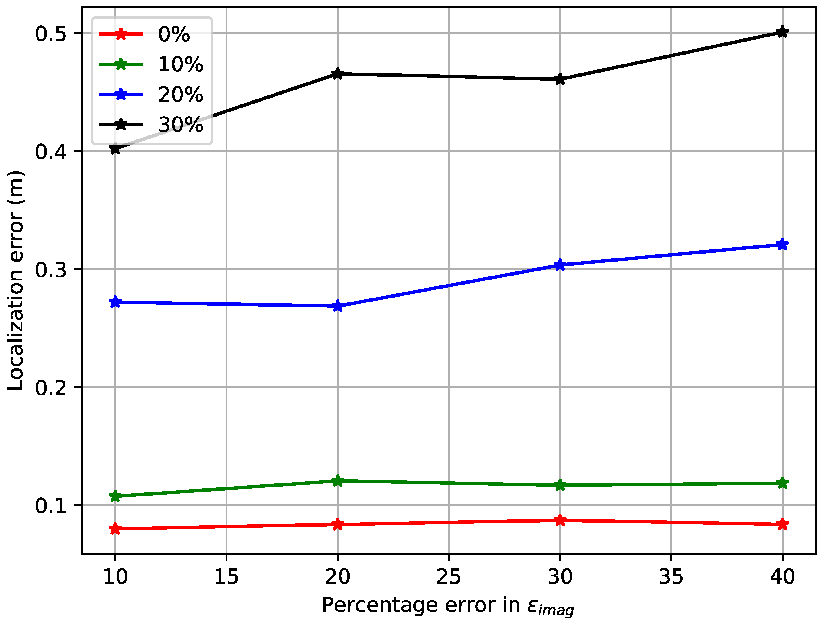
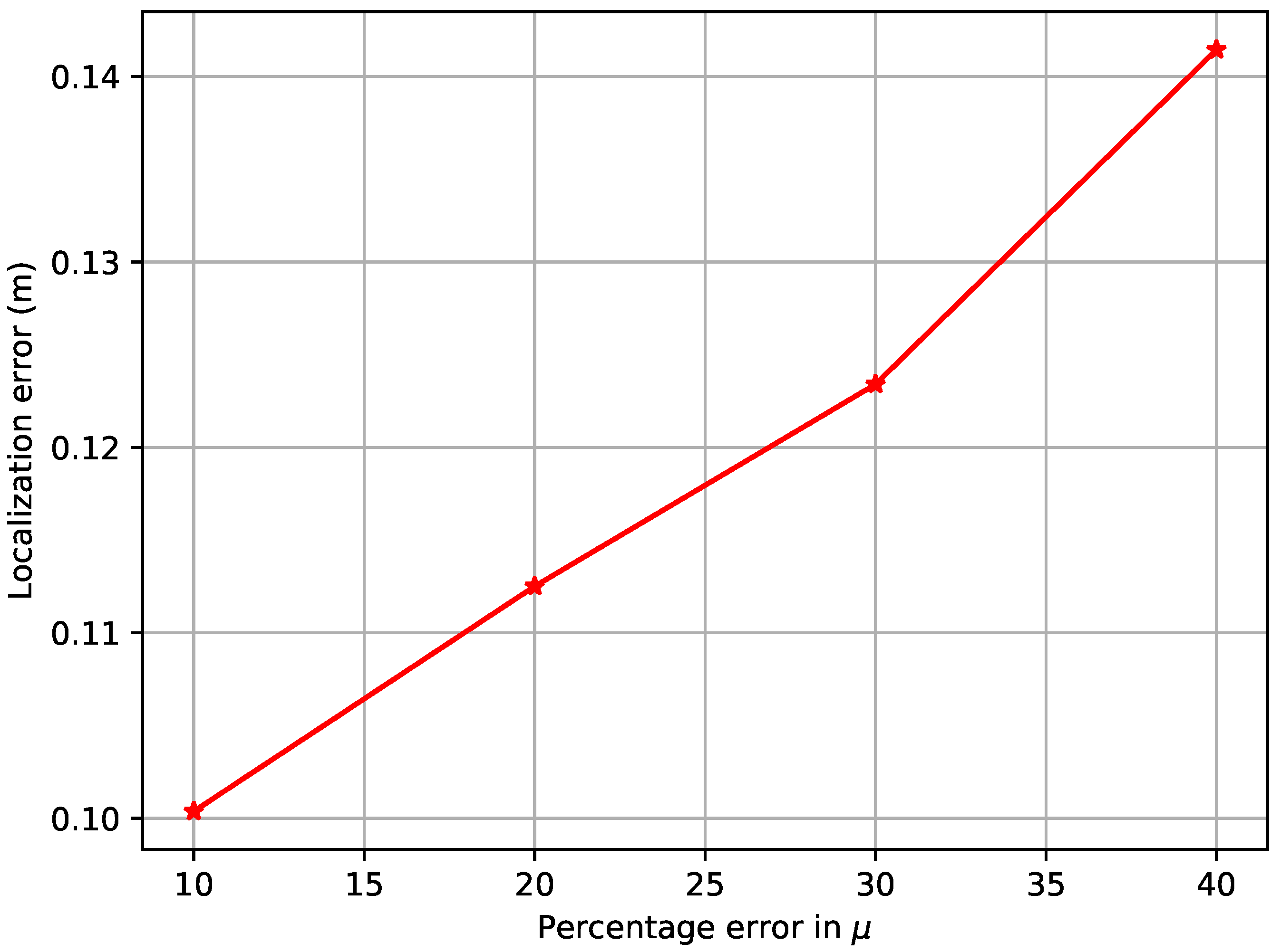
• We further validate our localization schemes with rigorous sensitivity analyses of the location estimates with respect to errors in measurements of various soil parameters.

1.1. Related Works

Range-based localization using measurements of time of arrival (ToA), angle of arrival (AoA) and received signal strength (RSS) has been well studied in literature. In [35], the authors develop statistical models to characterize such measurements to develop a peer to peer localization scheme for sensor nodes. In [36], authors use graph rigidity theory to develop conditions for unique localizability of sensor nodes in a network where some nodes’ locations are known. Nodes with unknown locations are localized based on a relative coordinate system formed by a few chosen nodes in the network in [37].

In [38], authors present a range-free localization scheme for a sensor network in an environment with obstacles or irregular coverage. In range-free approaches the localization accuracy suffers as the density of nodes decreases and there are obstacles in the signal propagation path. As an example of range-based localization, a detectable event (such as a burst of light or sound) is generated using an event disseminator and nodes report the detection of the events along with the timestamps to a central location server which computes the position of the nodes based on prior knowledge of the event propagation delays [39].

Range-based models for Ultra Wide Bandwidth (UWB) technology are used for cooperative localization techniques in [40] in which authors also present a localization algorithm by mapping a statistical model for graphical inference onto the network topology. A hybrid scheme using both range-based and range free methodology is presented in [41] which presents a sequential Monte Carlo localization method for a sensor network with mobile nodes using both range measurements and hop distance along with mobility information about the nodes.

Thus, research on sensor node localization has been a focused interest for the good part of the last two decades. However, most such significant advances have focused on applications where the nodes are assumed to be located in a homogeneous physical medium; usually air wherein free space wave propagation models have been assumed. Only recently have researchers started focusing on characterizing signal propagation in lossy dielectric media. In [42], authors present a study of the effect of various types of materials (rocks, minerals, etc.) found underground on magneto-inductive field propagation. They provide attenuation figures for various common underground materials for quasi-static low frequency magneto-inductive fields and propose guidelines for localization systems in terms of channel path-loss, operational frequencies, and bandwidth. However, the analysis is based on the assumption of near field propagation. The frequencies of interest (1 kHz, 100 kHz, and 1 MHz) are much lower than what we consider in the present work.

3D localization has also seen limited development. In [43], the authors propose an underground 3D positioning network for similar frequencies of interest in scenarios such as rescue missions in narrow and tortuous underground tunnels. The network of anchors is incrementally deployed, with only the location of a limited number of anchor nodes known at the time of deployment. The authors formulate a maximum likelihood estimate (MLE) problem to estimate the range and bearing angle of communication. The positions of incrementally deployed anchor nodes is iteratively estimated which leads to accumulating errors as the network depth increases. Our application is different in that the nodes in our network are deployed in a relatively uniform medium, with relatively unchanged positions for long periods of time. Moreover, the bulky triaxial coil antennae for magneto-inductive communication are not suitable for the size limited sensor nodes in our application.

In [44], authors derive a multi-sensor data attenuation model using radio, acoustic, and visible light signals and develop a model for real time mobile node tracking in an indoor building. The authors propose a compartmental model based on fluid movement in biological systems with interacting compartments. The model, having a higher number of parameters, is better able to model the path loss compared to log and exponential models. The problem is formulated as a least squares estimated problem by first linearizing the Taylor’s series expansion of the compartmental model and solving it using Singular Value Decomposition. The authors first propose a range free coarse estimator for initializing the node location and thereafter a real time node tracking method is presented. The model selectively combines the multi-sensor data based on the bandwidth utilization in the wireless channel.

In [45], a neural network-based localization problem formulation is proposed using Time Difference of Arrival (TDOA) as the ranging measurement. Two types of neural network models—Back Propagation Network (BPN) and Radial Basis Function (RBF)—are used. Most 3D localization for sensor nodes deployed underground has focused on mines, pipes, and tunnels ([46,47,48]). In [49], authors characterize the link quality and received signal strength for wireless sensor networks deployed for underground pipeline monitoring to gain insight into protocol development for wireless underground sensor networks (WUSNs).

Applications exist with varying degrees of localization accuracy needed. A trade-off is made among the localization hardware complexity, algorithm complexity, deployment costs, and localization accuracy. In [50], authors study the effect of error inducing parameters in localization. They derive the Cramer–Rao lower bound for multi-hop localization systems by studying the effect of parameters such as measurement technology accuracy, node density, beacon uncertainty, etc. on localization error.

Nature inspired swarm intelligence metaheuristic-based algorithms have also garnered interest in the field of localization as in [51,52,53,54,55]. In [51], authors present a study of the performance of nature inspired algorithms for localization such as Flower pollination algorithm, firefly algorithm, gray wolf optimization, and particle swarm optimization in terms of localization accuracy, number of nodes localized, and computation complexity. In [52], authors present a localization scheme that employs received signal strength indicator measurements for ranging using swarm intelligence firefly algorithm for optimization to estimate node locations. Authors in [53,54,55] propose localization approaches using elephant herding optimization, butterfly optimization, and hybridized moth search algorithms. While these are creative approaches to solving the node localization problem, they are also applied in the case where signal transmission happens through the medium of air only.

Some research has targeted localization of sensor nodes in different physical media such as underwater and underground mine deployed networks as in [56,57,58]. In [56], authors propose a multi-hop node localization scheme for underwater wireless sensor networks while using AoA and distance measurements with weighted least squares method. In [57], authors propose a method to improve localization in underground mines by proposing an anchor selection process based on values of received signal strength indicator. Authors in [58] propose a range free localization method for underwater acoustic sensor networks.

Our previous work in [32,33] addresses the problem of sensor node localization for nodes placed in multiple physical media using measurements of received signal strength. We have developed a probabilistic model for path loss of the radio frequency signal as it travels across the interface between two different physical media—air and soil. The model is parameterized in terms of the node locations and the localization problem is formulated as a maximum likelihood estimation.

2. Materials and Methods

In our study, the time difference between the transmission of a beacon signal (an unmodulated sinusoidal wave) at one node and its reception at another node is used to estimate the distance between the nodes. This delay is estimated using a matched filter at the receiving node, where a noise-free transmitted signal is available. The copy of the transmitted signal is delayed in time by a certain amount and its correlation with the received signal is measured for a certain observation time. The delay value at which the output of the correlator is maximum gives an estimate of the propagation delay between the transmitter and receiver. However, this estimate is uncertain owing to noise in the received signal. Furthermore, multi-path interference may cause additional uncertainty in the estimate. For background, we introduce the single-path case first.

2.1. MLE of ToA for a Single Path

We assume that the transmitted signal $s\left(t\right)$ is corrupted by additive white Gaussian noise $n\left(t\right)$ upon reception at the receiver node as $r\left(t\right)$, after a distance and medium dependent attenuation A and delay $\tau$:

$$r\left(t\right)=As(t-\tau )+n\left(t\right).$$

(1)

The auto-covariance function of the noise is $\mathbb{E}\left[n\left(t\right)n\left(t^{\prime }\right)\right]=\frac{N_0}{2}\delta (t-t^{\prime })$, where $\delta (·)$ is the dirac-delta function and $\frac{N_0}{2}$ is the noise power spectral density.

$r\left(t\right)$ is observed over an interval $[0,T]$ at the receiver node. To show that MLE based on ToA reduces to a matched filter described above, we proceed by discretization and then take the limit to get back to the continuous domain. Accordingly, let us consider the observed data consisting of $n+1$ equally spaced samples of $r\left(t\right)$, at time instants $t_k=k\Delta t$, where $t_0=0$, $t_n=n\Delta t=T$, and $k\in \{0,1,2,\dots ,n\}$. The individual samples $r_k$ are Gaussian random variables with mean $A{s}_k$ and variance $\frac{N_0}{2}\delta \left[0\right]=\frac{N_0}{2}$, where $s_k$ is a sample of the signal $s\left(t\right)$ at time $t_k-\tau$, defined as $s_k=s(t_k-\tau )$. The observed data-vector $\mathbf{r}$ has a multivariate-Gaussian distribution, where the joint-pdf is driven by the noise pdf. The covariance matrix $\Phi$ of $\mathbf{r}$ is $(n+1)$ by $(n+1)$, with ${\{j,k\}}^{th}$ element:

$${\varphi }_{jk}=\frac{N_0}{2}\delta [j-k],$$

(2)

where ${\varphi }_{jk}$ is the covariance between $r_j$ and $r_k$. The mean of $\mathbf{r}$ equals the samples of the transmitted signal:

$$\begin{array}{c}\hfill E\left[\mathbf{r}\right]=A\mathbf{s}:=A{[s_0\dots s_k\dots s_n]}^T,\end{array}$$

(3)

where ${}^T$ denotes the vector transpose operation. Thus, the joint-pdf of $\mathbf{r}$ is:

$$\begin{array}{cc}\hfill p\left(\mathbf{r}\right|\tau )& =\frac{1}{{\left(2\pi \right)}^{\frac{(n+1)}{2}}{|\Phi |}^{\frac{1}{2}}}exp\left\{\frac{-1}{2}{(\mathbf{r}-A\mathbf{s})}^T{\Phi }^{-1}(\mathbf{r}-A\mathbf{s})\right\},\hfill \end{array}$$

(4)

$$\begin{array}{cc}\hfill & =\frac{1}{{\left(\pi N_0\right)}^{\frac{(n+1)}{2}}}exp\left\{-\sum _{k=1}^{n+1}\frac{{(r_k-A{s}_k)}^2}{N_0}\right\},\hfill \end{array}$$

(5)

where Equation (5) follows from (4) by using (2), and substituting ${\varphi }_{jk}=\frac{N_0}{2}\delta [j-k]$ for additive white Gaussian noise.

Noting that the squared terms $r_k^2$ and ${\left(A{s}_k\right)}^2$ sum up to received and attenuated signal powers, which are independent of the delay of communication, the log-likelihood function, ignoring the terms that do not depend on $\tau$, is given by:

$$log\Lambda \left(\tau \right|\mathbf{r})=\sum _{k=1}^{n+1}\frac{2r_{k}A{s}_k}{N_0}.$$

(6)

Under the limit as $\Delta t\to 0$ (and $n\to \infty$), Equation (6) becomes:

$$\begin{array}{c}\hfill log\Lambda \left(\tau \right|r\left(t\right))={\int }_0^T\frac{2}{N_0}r\left(t\right)As(t-\tau )dt.\end{array}$$

(7)

Thus, the log-likelihood function reduces to the correlator function between $r\left(t\right)$ and $s\left(t\right)$ given a certain delay between the two, which is the output of a matched filter. Hence, $\hat{\tau }$ that maximizes this correlator function between the transmitted and received signals turns out to be the maximum likelihood estimate of the delay $\tau$.

The mean of $\hat{\tau }$, denoted by $\overline{\tau }$, is determined by the distance between the sender and receiver nodes and the propagation speed of the signal in the medium it travels. The variance of $\hat{\tau }$, being an MLE, asymptotically, as the sample size increases, equals the Cramer–Rao lower bound (CRLB) and is the inverse of the Fisher information matrix, given by [59]:

$$\begin{array}{cc}\hfill {\sigma }^2& ={\left[\mathbb{E}\left\{\frac{\partial }{\partial \tau }\left[log\Lambda \left(\tau \right|r\left(t\right))\right]\frac{\partial }{\partial \tau }\left[log\Lambda \left(\tau \right|r\left(t\right))\right]\right\}\right]}^{-1}\hfill \end{array}$$

(8)

The next expression follows from the derivation given in ([59], pp. 264–265),

$$\begin{array}{cc}\hfill {\sigma }^2& ={\left\{\frac{2A^2}{N_0}{\int }_0^T\frac{\partial }{\partial \tau }s(t-\tau )\frac{\partial }{\partial \tau }s(t-\tau )dt\right\}}^{-1}\hfill \end{array}$$

(9)

$$\begin{array}{cc}\hfill & ={\left\{\frac{2A^2}{N_0}{\int }_0^T{\left[s^{\prime }\left(t\right)\right]}^{2}dt\right\}}^{-1}\hfill \end{array}$$

(10)

$$\begin{array}{cc}\hfill & ={\left\{\frac{2A^2}{N_0}\int {\left(2\pi f\right)}^2{\left|S\left(f\right)\right|}^{2}df\right\}}^{-1}\hfill \end{array}$$

(11)

$$\begin{array}{cc}\hfill & ={\left\{8{\pi }^2\frac{p}{N_0}T{\beta }^2\right\}}^{-1},\hfill \end{array}$$

(12)

$$\begin{array}{cc}\hfill & ={\left\{8{\pi }^{2}TB{\beta }^2\mathrm{SNR}\right\}}^{-1}\hfill \end{array}$$

(13)

where $S\left(f\right)$ is the Fourier transform of the signal $s\left(t\right)$, and $A^2$ is the signal power attenuation due to propagation in the respective medium, so that $p=\frac{A^2\int {\left|S\left(f\right)\right|}^{2}df}{T}$ is received signal-power, $\beta =\sqrt{\frac{{\int }_0^T{f}^2{\left|S\left(f\right)\right|}^{2}df}{{\int }_0^T{\left|S\left(f\right)\right|}^{2}df}}$ is a function of the signal, B is the bandwidth of the signal and $\mathrm{SNR}=\frac{p}{N_{0}B}$ is the signal to noise power ratio. Thus, we have established that the variance of the time of arrival as estimated by the receiver’s matched filter, which is also the maximum likelihood estimate, is given by Equation (12). Since the MLE is asymptotically normal, the estimated time of arrival $\hat{\tau }$ can be approximated to be a Gaussian distributed random variable:

$$p_{\hat{\tau }}\left(\tau \right)=\frac{1}{\sqrt{2\pi {\sigma }^2}}{e}^{-\frac{{(\tau -\overline{\tau })}^2}{2{\sigma }^2}}.$$

(14)

2.2. Mean and Variance of Time of Arrival in Terms of Location Coordinates

In this section, we derive the relations that establish the dependence of $\overline{\tau }$ and ${\sigma }^2$ on the location coordinates of the sensor nodes. In this way, the pdf of $\hat{\tau }$ can be parameterized in terms of the location coordinates in order to estimate the latter from the observed times of arrival for signals transmitted between neighboring pairs of sensor nodes and between the sensor nodes and the satellite nodes. We provide the derivations for both the multi-path and multi-media cases in their respective sections.

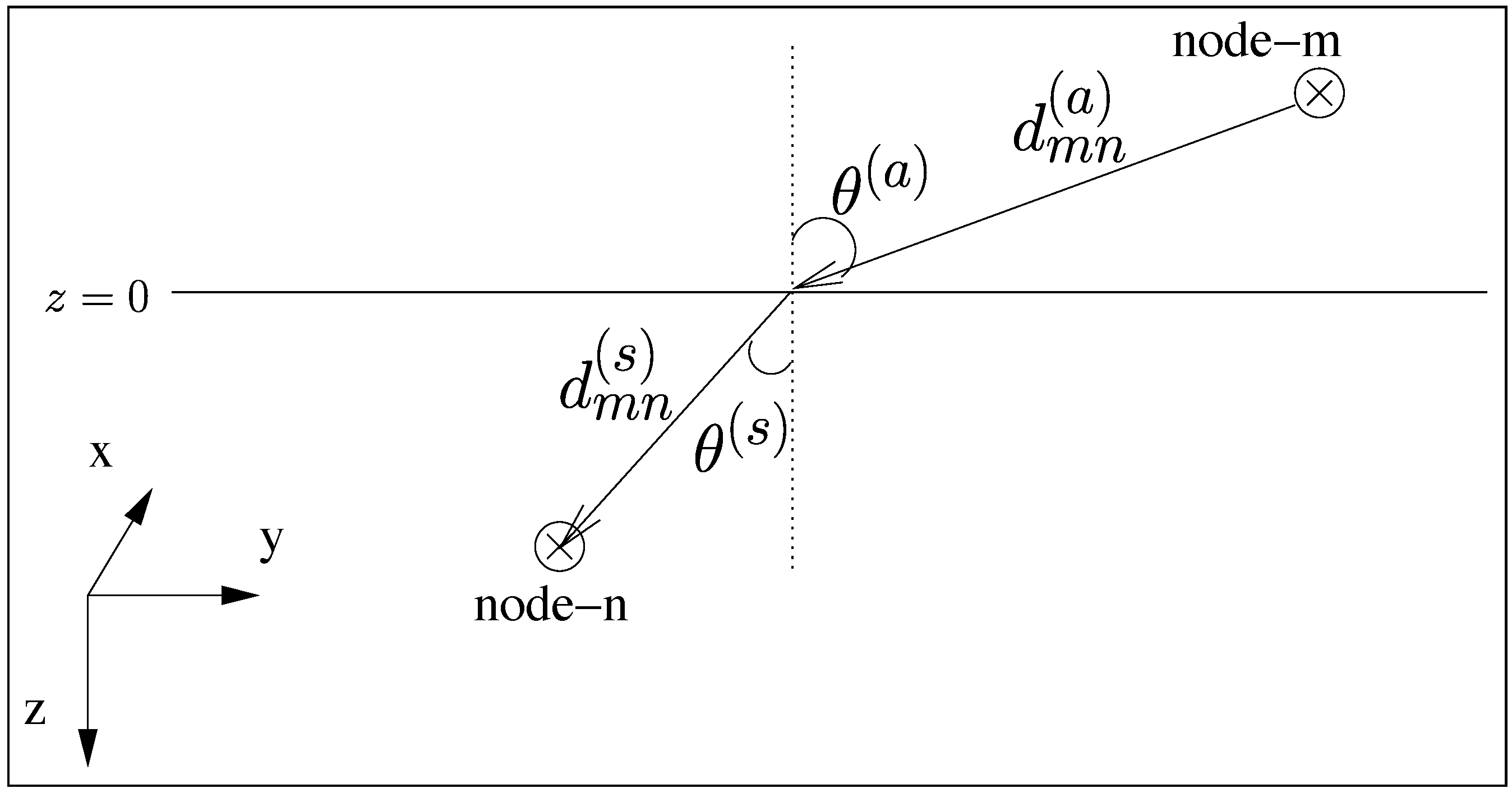
2.2.1. Multi-Path Extension: Soil-to-Soil Communication

As shown in Figure 1, a signal transmitted by an underground sensor node arrives at another underground sensor node via two paths; one along the direct line-of-sight path and another along a path after reflection from the ground surface. The received signal in time domain is given by:

$$r\left(t\right)=As(t-\tau )+A^{r}s(t-{\tau }^r)+n\left(t\right),$$

(15)

where A and $A^r$ are the attenuations along the two paths and $\tau$ and ${\tau }^r$ are the propagation delays along the two paths.

Following the steps in Section 2.1 for the received signal given by Equation (15), the joint log-likelihood function for the parameter $\mathit{\tau }={\left[\tau {\tau }^r\right]}^T$ is given by:

$$\begin{array}{c}\hfill log\Lambda \left(\mathit{\tau }\right|r\left(t\right))={\int }_0^T\frac{2}{N_0}r\left(t\right)\left\{As(t-\tau )+A^{r}s(t-{\tau }^r)\right\}dt.\end{array}$$

(16)

The estimate of $\mathit{\tau }$ that maximizes Equation (16) is the maximum likelihood estimate. Hence, the covariance matrix of the estimate is given by the inverse of the Fisher information matrix. The ${(i,j)}^{th}$ element of the covariance matrix ${\Sigma }_{2\times 2}$ is, then, given by:

$$\begin{array}{cc}\hfill {\sigma }_{ij}^2& ={\left[\mathbb{E}\left\{\frac{\partial }{\partial {\theta }_i}\left[log\Lambda \left(\mathit{\tau }\right|r\left(t\right))\right]\frac{\partial }{\partial {\theta }_j}\left[log\Lambda \left(\mathit{\tau }\right|r\left(t\right))\right]\right\}\right]}^{-1},\hfill \end{array}$$

(17)

where $i,j\in \{1,2\}$ corresponds to the line of sight and reflected paths; ${\theta }_1=\tau$ and ${\theta }_2={\tau }^r$.

Similar to the derivation of Equation (12), we have:

$$\begin{array}{cc}\hfill {\sigma }_{ij}^2& ={\left\{\frac{2A_i{A}_j}{N_0}{\int }_0^T\frac{\partial }{\partial {\theta }_i}s(t-{\theta }_i)\frac{\partial }{\partial {\theta }_j}s(t-{\theta }_j)dt\right\}}^{-1}\hfill \end{array}$$

(18)

$$\begin{array}{cc}\hfill & ={\left\{\frac{2A_i{A}_j}{N_0}{\int }_0^T{\left[s^{\prime }\left(t\right)\right]}^{2}dt\right\}}^{-1}\hfill \end{array}$$

(19)

$$\begin{array}{cc}\hfill & ={\left\{\frac{2A_i{A}_j}{N_0}\int {\left(2\pi f\right)}^2{\left|S\left(f\right)\right|}^{2}df\right\}}^{-1}\hfill \end{array}$$

(20)

$$\begin{array}{cc}\hfill & ={\left\{8{\pi }^2\frac{\sqrt{p_i}\sqrt{p_j}}{N_0}T{\beta }^2\right\}}^{-1},\hfill \end{array}$$

(21)

$$\begin{array}{cc}\hfill & ={\left\{8{\pi }^{2}TB{\beta }^2\sqrt{{\mathrm{SNR}}_i}\sqrt{{\mathrm{SNR}}_j}\right\}}^{-1},\hfill \end{array}$$

(22)

where ${\mathrm{SNR}}_i=\frac{p_i}{N_{0}B}$ and ${\mathrm{SNR}}_j=\frac{p_j}{N_{0}B}$ are the signal to noise power ratios for the two paths i and j. The expression for the received power for signal transmission in a lossy medium is discussed in the Appendix A in Equations (A1)–(A6). Accordingly, following (A6), we have:

$$\begin{array}{c}\hfill p_1=p_{mn}=\eta {\left(d_{mn}\right)}^{-k_s}{e}^{-2{\alpha }_s{d}_{mn}}\end{array}$$

(23)

$$\begin{array}{c}\hfill p_2=p_{mn}^r=\eta {\left(d_{mn}\right)}^{-k_s}{e}^{-2{\alpha }_s{d}_{mn}}\rho ,\end{array}$$

(24)

where the multiplicative constant reflection coefficient, $\rho$, reflected path is given by:

$$R={\left(\frac{\sqrt{{\mu }_a/{ϵ}_a^{\prime }}-\sqrt{{\mu }_s/{ϵ}_s^{\prime }}}{\sqrt{{\mu }_a/{ϵ}_a^{\prime }}+\sqrt{{\mu }_s/{ϵ}_s^{\prime }}}\right)}^2,$$

(25)

where ${ϵ}^{\prime }$ and $\mu$ are the real part of permittivity and permeability with ‘a’ and ‘s’ denoting air and soil media, respectively.

For sender–receiver pair $(m,n)$, the mean value ${\overline{\mathit{\tau }}}_{mn}={\left[{\overline{\tau }}_{mn}{\overline{\tau }}_{mn}^r\right]}^T$ is determined by the propagation distances and the speed of the signal:

$${\overline{\tau }}_{mn}=\frac{d_{mn}}{c_s},$$

(26)

$${\overline{\tau }}_{mn}^r=\frac{d_{mn}^{\left(r\right)}}{c_s},$$

(27)

where the line of sight propagation distance $d_{mn}$ and the reflected path propagation distance $d_{mn}^{\left(r\right)}$ are as shown in Figure 1 and the speed of light in soil $c_s$ is given by:

$$c_s=\frac{1}{\sqrt{\frac{{\mu }_s{ϵ}_s^{\prime }}{2}(\sqrt{1+{\left(\frac{{\sigma }_s}{\omega {ϵ}_s^{\prime }}\right)}^2}+1)}},$$

(28)

where ${ϵ}_s^{\prime }$, ${\mu }_s$ and ${\sigma }_s$ are, respectively, the real part of permittivity, permeability, and the conductivity of soil.

Following the same argument as in Section 2.1, $\hat{\mathit{\tau }}$ is asymptotically distributed as a bivariate Gaussian random variable with the pdf:

$$\begin{array}{cc}\hfill p_{{\hat{\mathit{\tau }}}_{mn}}\left({\mathit{\tau }}_{mn}\right)=& \frac{1}{\left(2\pi \right)|{\Sigma }_{mn}{|}^{1/2}}exp\left\{-\frac{1}{2}{({\mathit{\tau }}_{mn}-{\overline{\mathit{\tau }}}_{mn})}^T{\Sigma }_{mn}^{-1}\right.\hfill \\ \hfill & \left.({\mathit{\tau }}_{mn}-{\overline{\mathit{\tau }}}_{mn})\right\}.\hfill \end{array}$$

(29)

2.2.2. Multi-Media Extension: Air-to-Soil Communication

For signal propagation between a satellite node m and a sensor node n, the propagation medium is partly air and partly soil, see Figure 2, where $d_{mn}^{\left(a\right)}$ and $d_{mn}^{\left(s\right)}$, the propagation distances in air and soil, respectively, are computed as the solutions of the following two equations:

$$\begin{array}{cc}\hfill & \frac{d_{mn}^{\left(a\right)}}{\sqrt{{\left(d_{mn}^{\left(a\right)}\right)}^2-z_m^2}}\frac{\sqrt{{\left(d_{mn}^{\left(s\right)}\right)}^2-z_n^2}}{d_{mn}^{\left(s\right)}}\left(=\frac{sin{\theta }^{\left(a\right)}}{sin{\theta }^{\left(s\right)}}\right)=\frac{{\lambda }^{\left(a\right)}}{{\lambda }^{\left(s\right)}}\hfill \end{array}$$

(30)

$$\begin{array}{cc}\hfill & \sqrt{{\left(d_{mn}^{\left(a\right)}\right)}^2-z_m^2}+\sqrt{{\left(d_{mn}^{\left(s\right)}\right)}^2-z_n^2}=\sqrt{{(x_m-x_n)}^2+{(y_m-y_n)}^2},\hfill \end{array}$$

(31)

where ${\lambda }^{\left(a\right)}$ and ${\lambda }^{\left(s\right)}$ represent the wavelengths in air and soil, respectively. The above result follows from the application of the Snell’s law of refraction. Note that a satellite node is allowed to be anywhere above ground (an not necessarily on the ground), i.e., $z_m\ge 0$ (as opposed to $z_m=0$ necessarily).

As a result of the high refractive index of the soil compared to the air, the signal travels almost vertically downwards in the soil so as to minimize its sojourn time in the soil (this fact is also demonstrated by the small value of the Brewster’s angle for the soil-air interface [60]). Accordingly, we can obtain the following approximations:

$$\begin{array}{cc}\hfill d_{mn}^{\left(s\right)}& \approx z_n,\hfill \end{array}$$

(32)

$$\begin{array}{cc}\hfill d_{mn}^{\left(a\right)}& \approx \sqrt{{(x_m-x_n)}^2+{(y_m-y_n)}^2+z_m^2}.\hfill \end{array}$$

(33)

Therefore, we obtain an expression for the mean value of the propagation delay between the satellite and sensor nodes:

$${\overline{\tau }}_{mn}=\frac{d_{mn}^{\left(a\right)}}{c_a}+\frac{d_{mn}^{\left(s\right)}}{c_s},$$

(34)

where $c_a\approx c$ is the signal speed in air that approximately equals the speed of light in vacuum, and $c_s$ is given by Equation (28).

The variance in terms of the location coordinates, following Equation (12) is given by:

$$\begin{array}{cc}\hfill {\sigma }_{mn}^2& ={\left\{8{\pi }^2\frac{p_{mn}^{\left(as\right)}}{N_0}T{\beta }^2\right\}}^{-1}={\left\{8{\pi }^{2}TB{\beta }^2{\mathrm{SNR}}_{mn}\right\}}^{-1},\hfill \end{array}$$

(35)

where $p_{mn}^{\left(as\right)}$, the average received power for air-to-soil communication, is derived in terms of the location coordinates of the satellite node m and sensor node n,

$$\begin{array}{c}\hfill p_{mn}^{\left(as\right)}=\eta {\left(d_{mn}^{\left(a\right)}\right)}^{-k^{\left(a\right)}}{\left(d_{mn}^{\left(s\right)}\right)}^{-k^{\left(s\right)}}{e}^{-2{\alpha }^{\left(s\right)}{d}_{mn}^{\left(s\right)}}T,\end{array}$$

(36)

where $T=1-R$ is the transmission coefficient (R is given by Equation (25)).

2.3. MLE-Based Localization

Now we formulate a maximum likelihood problem to estimate the location coordinates of the nodes given the measurements of the times of arrivals at the nodes from their neighboring underground as well as above-ground satellite nodes.

Let $N_{ss}$ and $N_{as}$ denote the set of soil-to-soil and air-to-soil node pairs that communicate to gather the time of arrival data for soil-to-soil signal propagation and air-to-soil propagation, respectively. The log-likelihood of the time of arrival distribution parameters for all the sender-receiver pairs $(m,n)\in N_{ss}\cup N_{as}$ can be expressed as follows:

$$\begin{array}{cc}\hfill L\left(\mathsf{\Theta }\right|\mathit{T})& =-\sum _{(m,n)\in N_{as}}\left\{ln\left({\sigma }_{mn}\right)+\frac{{\left({\tau }_{mn}-{\overline{\tau }}_{mn}\right)}^2}{2{\sigma }_{{\hat{\tau }}_{mn}}^2}\right\}\hfill \\ \hfill & -\sum _{(m,n)\in N_{ss}}\left\{\frac{1}{2}ln\left|{\Sigma }_{mn}\right|+\frac{1}{2}{({\mathit{\tau }}_{mn}-{\overline{\mathit{\tau }}}_{mn})}^T{\Sigma }_{mn}^{-1}\right.\hfill \\ \hfill & \left.({\mathit{\tau }}_{mn}-{\overline{\mathit{\tau }}}_{mn})\right\},\hfill \end{array}$$

(37)

where $\mathit{T}$ represents the time of arrival data $\left\{{\tau }_{mn}\right|(m,n)\in N_{as},{\mathit{\tau }}_{mn}={\left[{\tau }_{mn}{\tau }_{mn}^r\right]}^T|(m,n)\in N_{ss}\}$ between all pairs of nodes that communicate with each other to gather localization data. ${\sigma }_{mn}$, ${\overline{\tau }}_{mn}$, ${\Sigma }_{mn}$, and ${\overline{\mathit{\tau }}}_{mn}={\left[{\overline{\tau }}_{mn}{\overline{\tau }}_{mn}^r\right]}^T$ were expressed in terms of the location coordinates of the sensor nodes and the known location coordinates of the satellite nodes in Section 2.2.1 and Section 2.2.2 for the different signal propagation scenarios in our application. Thus, the maximum likelihood estimates of the location coordinates are obtained as the values that maximize the log likelihood function given by Equation (37).

2.4. Software Implementation

The software used in this study is available at https://www.github.com/herman-ai/toalocalization (accessed on 26 November 2020). The software consists of python code files to perform localization, and also included is the code for sensitivity analysis. Readers may consult the included README file in the repository for detailed instructions on how to reproduce our results.

For the software implementation of our localization methodology, we built a simulation of the model that computes the ToA values of signals exchanged between different nodes, and this involved drawing from probability distributions derived through our simulation framework. However, note that in deployment, scheduling of the various transmissions were performed to ensure no collisions among the different signals. For drawing from the distribution of a ToA, we used the random module from the numpy package of Python. Next, during the optimization phase, we initialized the node locations to random values within the constraints of the field boundaries and using the observed values of the ToA (as sampled in the first phase of the simulations) minimized the maximum likelihood function as derived in (37) to estimate the true values of the nodes’ coordinates. For this purpose, we used the optimize module from the scipy package of Python.

3. Results

We validated our localization models and evaluate its performance using simulations. Our simulated sensor field consists of 25 sensor nodes spread evenly in a 100 m${}^2$ square field. The depth of the nodes is also randomly chosen between 0 and $0.5$ m. Soil moisture content affects the soil complex permittivity which governs the signal propagation. Our simulations are based on assumption of clay loam soil with a clay content of $20\%$. We used the computed values of real and imaginary parts of the permittivity for this soil type from [61] for various values of soil moisture content as given in

Table 1. Real and imaginary parts of relative permittivity of soil for different moisture contents.

Fractional Volume of Water	${\mathit{ϵ}}_{\mathit{s}}^{\prime }$	${\mathit{ϵ}}_{\mathit{s}}^{″}$
$0\%$	2.36	0.0966
$10\%$	5.086	0.441
$30\%$	16.410	2.368
$40\%$	24.485	3.857

.

Table 2. Parameters used in the simulations for localization.

Parameter	Symbol	Value
Transmit power (Satellite node)	$P^{\left(a\right)}$	38 dBm
Transmit power (Sensor node)	$P^{\left(s\right)}$	10 dBm
Thermal noise	$N_0$	−110 dBm
Path loss factor (air)	$k_a$	2
Path loss factor (soil)	$k_s$	2
Relative permeability (soil)	${\mu }_s$	1.0084
Frequency	f	433 MHz
Wavelength	$\lambda$	0.7 m
Bandwidth	B	1 Hz
Signal duration	$T_S$	1 ms

details the remaining parameters used in the simulations. Note the theoretical approach developed in the paper is independent of the parameters used including the working frequency value (433 MHz), one that we selected since it lies in the open communication band and only as a proof-of-concept. The relative permeability of soil is assumed to be 1, a reasonable value for soils not containing significant amount of iron [62]. Thermal noise is assumed to be $-110$ dBm based on standard receiver sensitivity [63]. The underground transmission range is approximately 34 m in dry soil at a transmission power level of 30 dBm, yielding to an average of 3 neighbors per sensor node, whereas the air-to-soil transmission range is approximately 1000 m, as computed using the average received signal strength expressions given in Equations (23), (24) and (36).

We followed a hierarchical estimation methodology for estimating the location coordinates in our scheme. First, we applied the air-to-soil model on the signals transmitted between the satellite nodes and the underground nodes to arrive at crude level location estimates. As the second stage, we applied the combined air-to-soil and soil-to-soil models, adding data from the signals exchanged among neighboring underground nodes to further refine the estimates.

Table 3. Comparison of achieved localization accuracy.

	TOA		RSS
Moisture Content	xy	z	xy	z
0%	$7.598\times {10}^{-2}$	$2.164\times {10}^{-3}$	$3.455\times {10}^{-1}$	$3.329\times {10}^{-1}$
10%	$1.049\times {10}^{-1}$	$2.148\times {10}^{-3}$	$3.568\times {10}^{-1}$	$3.355\times {10}^{-1}$
20%	$2.185\times {10}^{-1}$	$2.616\times {10}^{-3}$	$3.848\times {10}^{-1}$	$3.368\times {10}^{-1}$
30%	$3.661\times {10}^{-1}$	$3.908\times {10}^{-3}$	$4.225\times {10}^{-1}$	$3.341\times {10}^{-1}$

compares the errors in the location estimates obtained using the proposed approach based on time of arrival with the approach based on received signal strength proposed in [33] for various soil moisture concentrations. It is apparent that time of arrival-based localization results in up to two orders of magnitudes improvement in the localization error.

We used a minimal setup of our network to perform variance analysis of our location estimates: five sensor nodes deployed randomly within a square field of size 10 m × 10 m within the radio communication ranges of each other and four satellite nodes so that we can closely capture the real world deployment scenario where each sensor node has 3–4 neighboring sensor nodes. Then, we computed the mean sample standard deviation of the location estimate of the sensor nodes.

Figure 3 shows the variation of localization error in the X–Y plane and Z-direction for the location estimate of each sensor node with the moisture content of the soil. With the increase in the soil moisture content, the attenuation in the RF signal increases reducing the SNR which causes an increase in the variance of the time of arrival. In addition, note that as the soil moisture content increases the range of transmission of the localization signal decreases reducing the number of neighboring nodes that a sensor node can hear from and improve upon its location estimate. Thus, the localization accuracy decreases with the increase in the moisture content of the soil. Nevertheless, the accuracy in such cases can be increased by increasing the transmission range of more densely scattering the sensor nodes.

The localization accuracy using time of arrival-based ranging requires an added provision of clock synchronization among all the nodes in the network. Indeed, the clock synchronization is built into our network as it is also needed for scheduling [28,29]. Thus, boundedness of clock drifts can be guaranteed by resynchronizing the sensor nodes ahead of collecting the localization data. We studied the effect of the drift in sensors’ clocks in Figure 4. The X-axis represents the maximum drift in the sensors’ clocks from true time in either direction. We used a uniform random number generator to simulate the clock drifts, and as seen in Figure 4, the clock drift increases the localization error increases linearly.

Figure 5 shows the localization error as a function of the sampling duration. As the sampling duration increases, the accuracy of the time of arrival estimate increases as per Equations (21) and (35). Accordingly, the accuracy of the estimates of the location coordinates increases as confirmed by Figure 5.

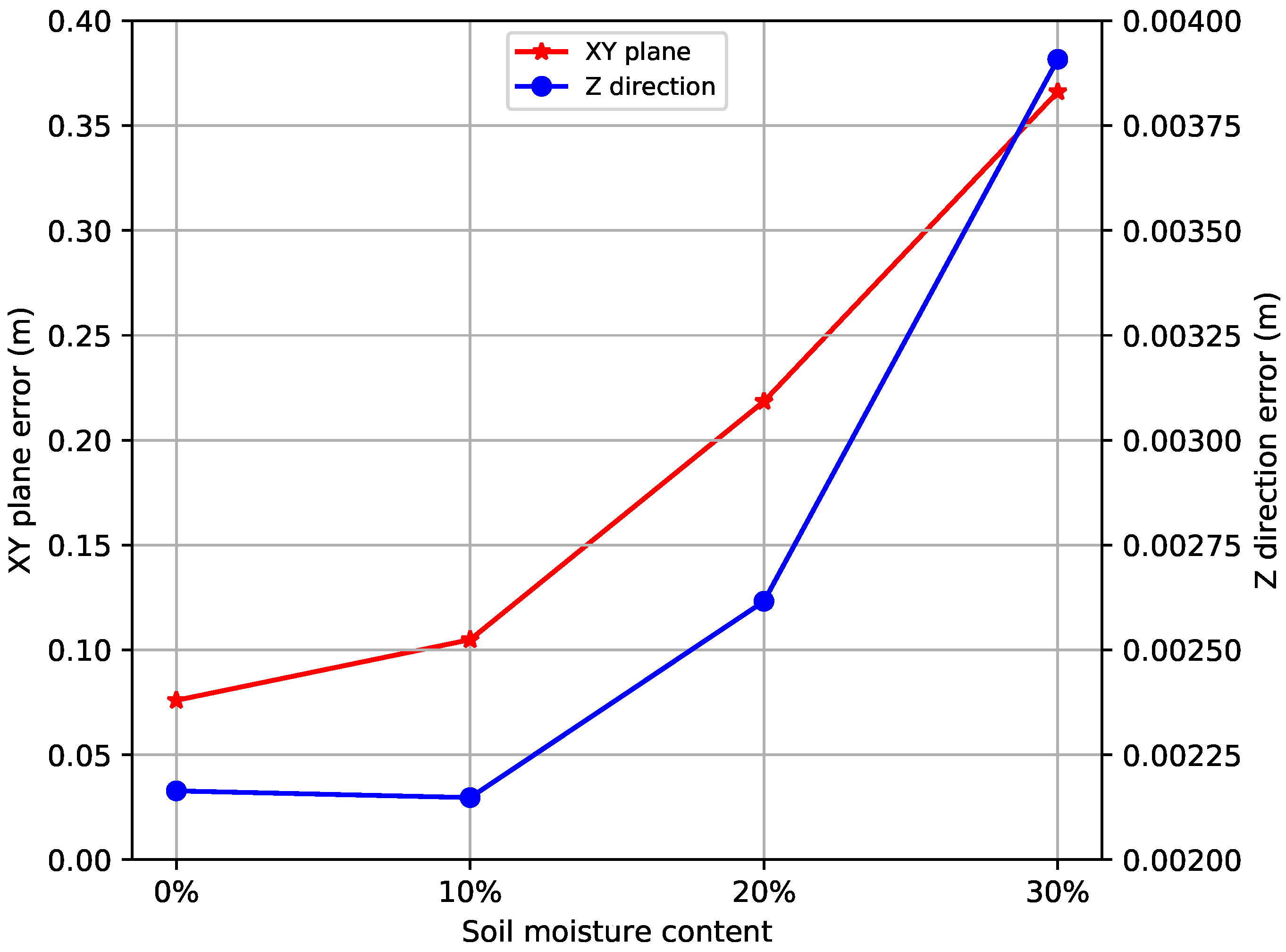
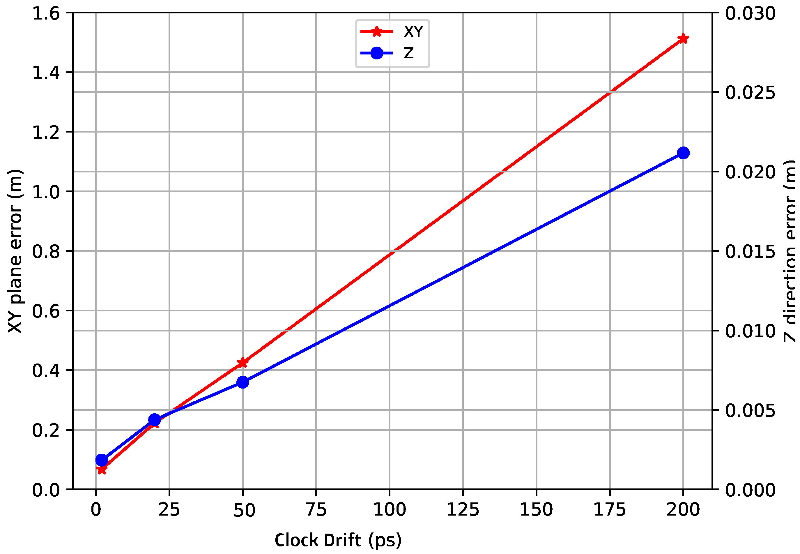
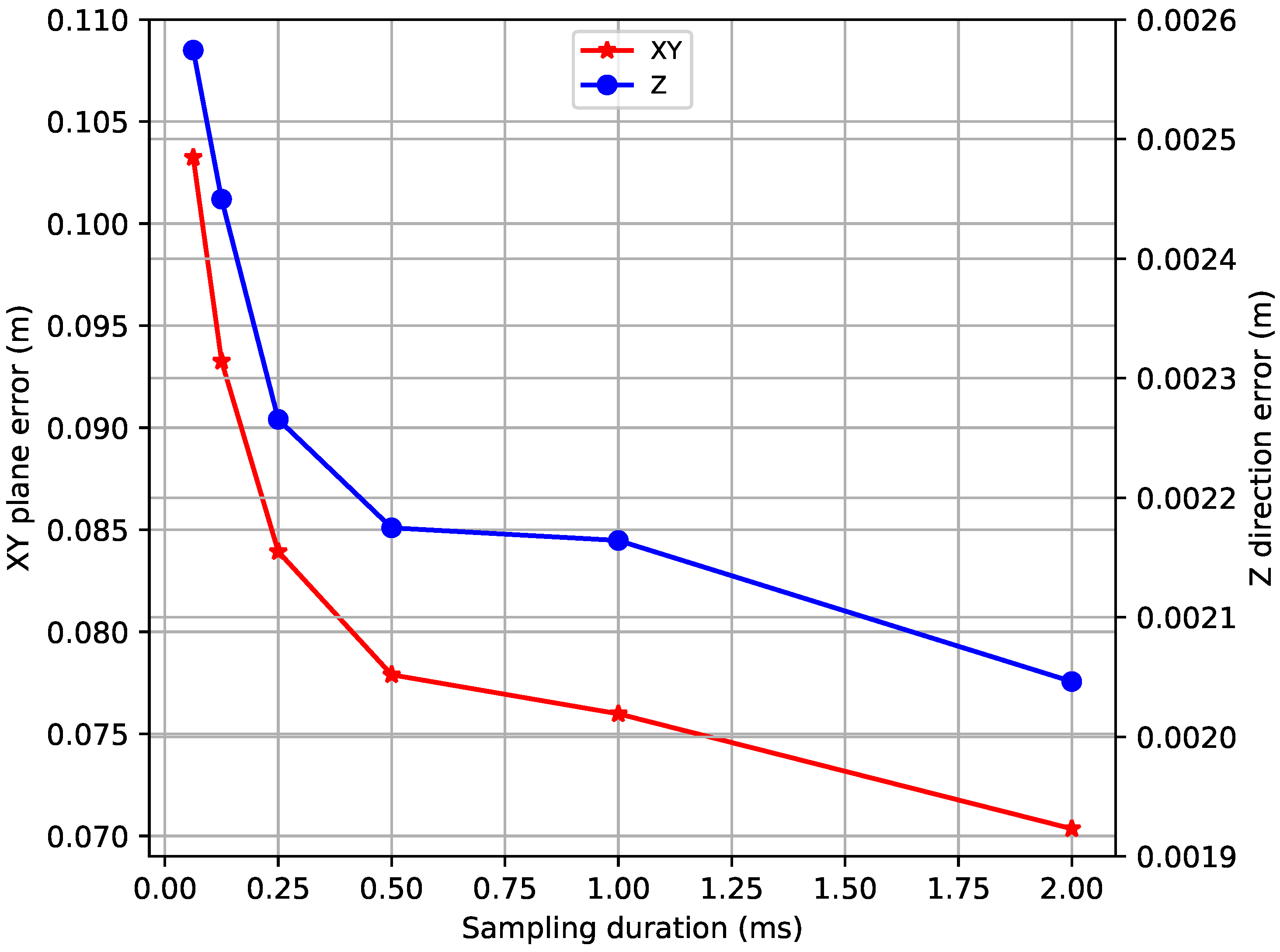
Sensitivity Analysis

Here we quantify the error induced in the location estimates due to uncertainty in various parameters of the localization models. The parameters of interest for our sensitivity analysis are soil permittivity and permeability. Errors in measurement of these parameters negatively impact the accuracy of the location estimates. We studied the change in the mean of the location estimates per unit shift in the measured values of ${\mu }_s$, ${ϵ}_s^{\prime }$ and ${ϵ}_s^{″}$ from their true values as shown in Table 1 and Table 2.

Figure 6, Figure 7 and Figure 8 present the sensitivities of the estimates to ${ϵ}_s^{\prime }$, ${ϵ}_s^{″}$, and ${\mu }_s$, respectively. Figure 6 shows that localization error is most sensitive to the estimate of the real part of soil permittivity. A shift of up to $40\%$ in the estimate of ${ϵ}_{real}$ is tolerable to maintain the localization error within 1 m for dry soil. Figure 7 shows that the localization estimate is relatively insensitive to the imaginary part of the soil permittivity for lower soil moisture content. This is due to the fact that for dry soil the real part of the soil permittivity dominates the imaginary part; in other words, the effect of soil conductivity is ignorable. Figure 8 shows that the localization estimate is also relatively less sensitive to the drift in the estimate of the magnetic permeability of soil. A $40\%$ drift in the permeability only causes an error of $40\%$ in the localization estimate.

4. Discussion

Our simulation results demonstrate that our technique is scalable and reliable. Although the results are presented for a field size of 10 m × 10 m, the technique is equally applicable to larger fields. This is because the complexity of the optimization problem used to solve for the location estimates only depends on the number of immediate neighbors and the anchor nodes in the field, both of which are upper bounded by a fixed number.

Note to further minimize the effect of synchronization drift between the nodes’ clocks one could further use round trip propagation time instead of time of arrival. In such a scheme, for example, Node A would send a pulse first to initiate the time of arrival data collection from Node B, which would respons immediately with another pulse back to Node A. Node A would measure the round trip time which would include delays due to transceiver circuitry and computational logic (and is relatively insensitive to the drift between the nodes’ clocks). Time of arrival estimate between these two nodes would equal half of the round trip time thus measured minus the hardware/software processing delay which can be estimated for the given hardware and software design.

Our experimental results showed the scalability of our MLE-based approach to practical sized sensor fields. For other application domains, where scalability may become an issue, other approaches may be explored. For example, to speed up the computation of the estimates at the expense of their accuracy one can formulate estimation as a method-of-moments problem. Such alternative formulations of the problem can be studied for analyzing the trade-off between the computational cost versus accuracy.

5. Conclusions

In this paper, we presented our study of sensor node localization for a wireless sensor network with anchor nodes placed above ground and sensor nodes deployed below ground surface. We presented our methodology of 3D localization of sensor node locations to compute their horizontal X and Y positions along with their depth Z under the ground surface. We used time of arrival of the signal between neighboring underground sensor nodes and between overground satellite nodes and sensor nodes for estimating the inter-node distances. Nodes located above ground, called satellite nodes, serve as anchor nodes in the scheme. We validated the localization model using simulations with realistic values of physical properties of the soil media with reasonable fluctuations due to moisture content. Location estimation errors in soil physical properties were also quantified using sensitivity analyses.

We developed a statistical model for the variation of the time of arrival of a radio frequency signal propagating along multiple physical media. The measured time of arrival is found to be Gaussian distributed with mean as a function of internode distances, and the variance a function of signal shape, duration, bandwidth, and SNR. Node localization is posed as a maximum likelihood estimation problem. Time of arrival measurements provided an accurate ranging solution for localization. In our previous work reported in [32,33] we tackled the 3D localization problem for multiple media using measurements of received signal strength as the ranging method. To the best of our knowledge, this is the first work (in conjunction with our prior work in [33]) for sensor node localization where nodes are located in different physical media, and accordingly the models have also been developed for the range measurements across multiple media. The improvement in localization accuracy as compared to those in [32,33] needs the added provision of clock synchronization, which is in-built in our framework and maintained by the routing and MAC layers in our design [30]. The shift in the detected time of arrival due to computation delays can be bounded by hardware and software design.

Future work requires field experiments to calibrate the parameters of the localization model, and indeed conducting a field-work is in the scope of future work for both sensor operation as well as its network operation validation. The current work lays the theoretical foundation and provides its proof-of-concept.

References

1. Xu, Z.; Dong, L.; Kumar, R. Electrophoretic Soil Nutrient Sensor for Agriculture. U.S. Patent 10,564,122, 18 February 2020. [Google Scholar]
2. Kumar, R.; Weber, R.J.; Pandey, G. Low RF-Band Impedance Spectroscopy Based Sensor for in-situ, Wireless Soil Sensing. U.S. Patent 10,073,074, 18 September 2018. [Google Scholar]
3. Pandey, G.; Weber, R.J.; Kumar, R. Agricultural cyber-physical system: In-situ soil moisture and salinity estimation by dielectric mixing. IEEE Access 2018, 6, 43179–43191. [Google Scholar] [CrossRef]
4. Xu, Z.; Wang, X.; Weber, R.J.; Kumar, R.; Dong, L. Nutrient sensing using chip scale electrophoresis and in situ soil solution extraction. IEEE Sens. J. 2017, 17, 4330–4339. [Google Scholar] [CrossRef]
5. Ali, M.A.; Jiang, H.; Mahal, N.K.; Weber, R.J.; Kumar, R.; Castellano, M.J.; Dong, L. Microfluidic impedimetric sensor for soil nitrate detection using graphene oxide and conductive nanofibers enabled sensing interface. Sens. Actuators B Chem. 2017, 239, 1289–1299. [Google Scholar] [CrossRef] [Green Version]
6. Xu, Z.; Wang, X.; Weber, R.J.; Kumar, R.; Dong, L. Microfluidic eletrophoretic ion nutrient sensor. In Proceedings of the 2016 IEEE SENSORS, Orlando, FL, USA, 30 October–3 November 2016; pp. 1–3. [Google Scholar]
7. Pandey, G.; Wang, K.N.; Kumar, R.; Weber, R.J. Employing a metamaterial inspired small antenna for sensing and transceiving data in an underground soil sensor equipped with a GUI for end-user. In Proceedings of the 2014 IEEE International Conference on Systems, Man, and Cybernetics (SMC), IEEE, San Diego, CA, USA, 5–8 October 2014; pp. 3423–3428. [Google Scholar]
8. Britz, B.; Ng, E.; Jiang, H.; Xu, Z.; Kumar, R.; Dong, L. Smart nitrate-selective electrochemical sensors with electrospun nanofibers modified microelectrode. In Proceedings of the 2014 IEEE International Conference on Systems, Man, and Cybernetics (SMC), IEEE, San Diego, CA, USA, 5–8 October 2014; pp. 3419–3422. [Google Scholar]
9. Pandey, G.; Kumar, R.; Weber, R.J. A low profile, low-RF band, small antenna for underground, in-situ sensing and wireless energy-efficient transmission. In Proceedings of the 11th IEEE International Conference on Networking, Sensing and Control, IEEE, Miami, FL, USA, 7–9 April 2014; pp. 179–184. [Google Scholar]
10. Pandey, G.; Kumar, R.; Weber, R.J. Design and implementation of a self-calibrating, compact micro strip sensor for in-situ dielectric spectroscopy and data transmission. In Proceedings of the SENSORS, 2013 IEEE, Baltimore, MD, USA, 3–6 November 2013; pp. 1–4. [Google Scholar]
11. Pandey, G.; Kumar, R.; Weber, R.J. Real time detection of soil moisture and nitrates using on-board in-situ impedance spectroscopy. In Proceedings of the 2013 IEEE International Conference on Systems, Man, and Cybernetics, IEEE, Manchester, UK, 13–16 October 2013; pp. 1081–1086. [Google Scholar]
12. Pandey, G.; Kumar, R.; Weber, R.J. Determination of soil ionic concentration using impedance spectroscopy. In Sensing Technologies for Global Health, Military Medicine, and Environmental Monitoring III; International Society for Optics and Photonics: Bellingham, WA, USA, 2013; Volume 8723, p. 872317. [Google Scholar]
13. Pandey, G.; Kumar, R.; Weber, R.J. A multi-frequency, self-calibrating, in-situ soil sensor with energy efficient wireless interface. In Sensing for Agriculture and Food Quality and Safety V; International Society for Optics and Photonics: Bellingham, WA, USA, 2013; Volume 8721, p. 87210V. [Google Scholar]
14. Kumar, R.; Tabassum, S.; Dong, L. Nano-Patterning Methods Including: (1) Patterning of Nanophotonic Structures at Optical Fiber tip for Refractive Index Sensing and (2) Plasmonic Crystal Incorporating Graphene Oxide Gas Sensor for Detection of Volatile Organic Compounds. U.S. Patent 10,725,373, 28 July 2020. [Google Scholar]
15. Kashyap, B.; Kumar, R. Sensing Methodologies in Agriculture for Soil Moisture and Nutrient Monitoring. IEEE Access 2021, 9, 14095–14121. [Google Scholar] [CrossRef]
16. Tabassum, S.; Dong, L.; Kumar, R. Determination of dynamic variations in the optical properties of graphene oxide in response to gas exposure based on thin-film interference. Opt. Express 2018, 26, 6331–6344. [Google Scholar] [CrossRef] [PubMed]
17. Tabassum, S.; Kumar, R.; Dong, L. Nanopatterned optical fiber tip for guided mode resonance and application to gas sensing. IEEE Sens. J. 2017, 17, 7262–7272. [Google Scholar] [CrossRef]
18. Tabassum, S.; Kumar, R.; Dong, L. Plasmonic crystal-based gas sensor toward an optical nose design. IEEE Sens. J. 2017, 17, 6210–6223. [Google Scholar] [CrossRef]
19. Tabassum, S.; Kumar, R. Selective Detection of Ethylene Using a Fiber-Optic Guided Mode Resonance Device: In-Field Crop/Fruit Diagnostics. In CLEO: Applications and Technology; Optical Society of America: Washington, DC, USA, 2020; p. ATu4I.6. [Google Scholar]
20. Kashyap, B.; Kumar, R. Bio-agent free electrochemical detection of Salicylic acid. In Proceedings of the 2019 IEEE SENSORS, Montreal, QC, Canada, 27–30 October 2019; pp. 1–4. [Google Scholar]
21. Kashyap, B.; Kumar, R. Salicylic acid (SA) detection using bi-enzyme microfluidic electrochemical sensor. In Smart Biomedical and Physiological Sensor Technology XV; International Society for Optics and Photonics: Bellingham, WA, USA, 2018; Volume 10662, p. 106620K. [Google Scholar]
22. Tabassum, S.; Wang, Q.; Wang, W.; Oren, S.; Ali, M.A.; Kumar, R.; Dong, L. Plasmonic crystal gas sensor incorporating graphene oxide for detection of volatile organic compounds. In Proceedings of the 2016 IEEE 29th International Conference on Micro Electro Mechanical Systems (MEMS), IEEE, Shanghai, China, 24–28 January 2016; pp. 913–916. [Google Scholar]
23. Bhar, A.; Kumar, R.; Qi, Z.; Malone, R. Coordinate descent based agricultural model calibration and optimized input management. Comput. Electron. Agric. 2020, 172, 105353. [Google Scholar] [CrossRef]
24. Bhar, A.; Kumar, R.; Malone, R.W. Comparing a Simple Carbon Nitrogen Model with Complex RZWQM Model. In Proceedings of the 2019 ASABE Annual International Meeting, American Society of Agricultural and Biological Engineers, Boston, MA, USA, 7–10 July 2019; p. 1. [Google Scholar]
25. Bhar, A.; Kumar, R. Model-Predictive Real-Time Fertilization and Irrigation Decision-Making Using RZWQM. In Proceedings of the 2019 ASABE Annual International Meeting, Boston, MA, USA, 7–10 July 2019; p. 1. [Google Scholar]
26. Dimakis, A.; Sarwate, A.; Wainwright, M. Geographic Gossip: Efficient Averaging for Sensor Networks. Signal Process. IEEE Trans. 2008, 56, 1205–1216. [Google Scholar] [CrossRef] [Green Version]
27. Zeng, K.; Ren, K.; Lou, W.; Moran, P.J. Energy aware efficient geographic routing in lossy wireless sensor networks with environmental energy supply. Wirel. Netw. 2009, 15, 39–51. [Google Scholar] [CrossRef]
28. Sahota, H.; Kumar, R.; Kamal, A.; Huang, J. An energy-efficient wireless sensor network for precision agriculture. In Proceedings of the IEEE Symposium on Computers and Communications, Riccione, Italy, 22–25 June 2010; pp. 347–350. [Google Scholar]
29. Sahota, H.; Kumar, R.; Kamal, A. Performance modeling and simulation studies of MAC protocols in sensor network performance. In Proceedings of the International Conference on Wireless Communications and Mobile Computing, ACM, Istanbul, Turkey, 5–8 July 2011. [Google Scholar]
30. Sahota, H.; Kumar, R.; Kamal, A. A wireless sensor network for precision agriculture and its performance. Wirel. Commun. Mob. Comput. 2011, 11, 1628–1645. [Google Scholar] [CrossRef]
31. Ren, K.; Lou, W.; Zhang, Y. LEDS: Providing Location-Aware End-to-End Data Security in Wireless Sensor Networks. Mob. Comput. IEEE Trans. 2008, 7, 585–598. [Google Scholar] [CrossRef]
32. Sahota, H.; Kumar, R. Network based sensor localization in multi-media application of precision agriculture Part 1: Received signal strength. In Proceedings of the 11th IEEE International Conference on Networking, Sensing and Control, Miami, FL, USA, 7–9 April 2014; pp. 191–196. [Google Scholar] [CrossRef]
33. Sahota, H.; Kumar, R. Maximum-Likelihood Sensor Node Localization Using Received Signal Strength in Multimedia with Multipath Characteristics. IEEE Syst. J. 2016, 12, 1–10. [Google Scholar] [CrossRef]
34. Sahota, H.; Kumar, R. Network based sensor localization in multi-media application of precision agriculture Part 2: Time of arrival. In Proceedings of the 11th IEEE International Conference on Networking, Sensing and Control, Miami, FL, USA, 7–9 April 2014; pp. 203–208. [Google Scholar] [CrossRef]
35. Patwari, N.; Ash, J.; Kyperountas, S.; Hero, A.O.; Moses, R.; Correal, N. Locating the nodes: Cooperative localization in wireless sensor networks. Signal Process. Mag. IEEE 2005, 22, 54–69. [Google Scholar] [CrossRef]
36. Aspnes, J.; Eren, T.; Goldenberg, D.; Morse, A.; Whiteley, W.; Yang, Y.; Anderson, B.; Belhumeur, P. A Theory of Network Localization. Mob. Comput. IEEE Trans. 2006, 5, 1663–1678. [Google Scholar] [CrossRef]
37. Youssef, A.; Agrawala, A.; Younis, M. Accurate anchor-free node localization in wireless sensor networks. In Proceedings of the 24th IEEE International Performance, Computing, and Communications Conference, Phoenix, AZ, USA, 7–9 April 2005; pp. 465–470. [Google Scholar] [CrossRef] [Green Version]
38. Xiao, B.; Chen, L.; Xiao, Q.; Li, M. Reliable Anchor-Based Sensor Localization in Irregular Areas. Mob. Comput. IEEE Trans. 2010, 9, 60–72. [Google Scholar] [CrossRef]
39. Stoleru, R.; He, T.; Mathiharan, S.; George, S.; Stankovic, J. Asymmetric Event-Driven Node Localization in Wireless Sensor Networks. Parallel Distrib. Syst. IEEE Trans. 2012, 23, 634–642. [Google Scholar] [CrossRef] [Green Version]
40. Wymeersch, H.; Lien, J.; Win, M. Cooperative Localization in Wireless Networks. Proc. IEEE 2009, 97, 427–450. [Google Scholar] [CrossRef]
41. Dil, B.; Dulman, S.; Havinga, P. Range-based localization in mobile sensor networks. In Wireless Sensor Networks; Springer: Berlin/Heidelberg, Germany, 2006; pp. 164–179. [Google Scholar]
42. Abrudan, T.E.; Kypris, O.; Trigoni, N.; Markham, A. Impact of Rocks and Minerals on Underground Magneto-Inductive Communication and Localization. IEEE Access 2016, 4, 3999–4010. [Google Scholar] [CrossRef]
43. Abrudan, T.E.; Xiao, Z.; Markham, A.; Trigoni, N. Underground Incrementally Deployed Magneto-Inductive 3-D Positioning Network. IEEE Trans. Geosci. Remote Sen. 2016, 54, 4376–4391. [Google Scholar] [CrossRef]
44. Kumar, S.; Hegde, R.M. An Efficient Compartmental Model for Real-Time Node Tracking Over Cognitive Wireless Sensor Networks. IEEE Trans. Signal Process. 2015, 63, 1712–1725. [Google Scholar] [CrossRef]
45. Singh, P.; Agrawal, S. TDOA Based Node Localization in WSN Using Neural Networks. In Proceedings of the 2013 International Conference on Communication Systems and Network Technologies, Gwalior, India, 6–8 April 2013; pp. 400–404. [Google Scholar] [CrossRef]
46. Wu, D.; Chatzigeorgiou, D.; Youcef-Toumi, K.; Ben-Mansour, R. Node Localization in Robotic Sensor Networks for Pipeline Inspection. IEEE Trans. Ind. Inform. 2016, 12, 809–819. [Google Scholar] [CrossRef]
47. Mao, Y.; Cheng, D. A localization algorithm by dynamic path-loss fading index for intelligent mining system. In Proceedings of the 2014 9th International Conference on Computer Science & Education, Vancouver, BC, Canada, 22–24 August 2014; pp. 977–980. [Google Scholar]
48. Assaf, A.E.; Zaidi, S.; Affes, S.; Kandil, N. Accurate Sensors Localization in Underground Mines or Tunnels. In Proceedings of the 2015 IEEE International Conference on Ubiquitous Wireless Broadband (ICUWB), Montreal, QC, Canada, 4–7 October 2015; pp. 1–6. [Google Scholar] [CrossRef]
49. Silva, B.; Fisher, R.M.; Kumar, A.; Hancke, G.P. Experimental Link Quality Characterization of Wireless Sensor Networks for Underground Monitoring. IEEE Trans. Ind. Inform. 2015, 11, 1099–1110. [Google Scholar] [CrossRef] [Green Version]
50. Savvides, A.; Garber, W.; Moses, R.; Srivastava, M. An analysis of error inducing parameters in multihop sensor node localization. Mob. Comput. IEEE Trans. 2005, 4, 567–577. [Google Scholar] [CrossRef]
51. Kaur, R.; Arora, S. Nature Inspired Range Based Wireless Sensor Node Localization Algorithms. Int. J. Inter. Multimed. Artif. Intell. 2017, 4, 7–17. [Google Scholar] [CrossRef] [Green Version]
52. Tuba, E.; Tuba, M.; Beko, M. Two stage wireless sensor node localization using firefly algorithm. In Smart Trends in Systems, Security and Sustainability; Springer: Berlin/Heidelberg, Germany, 2018; pp. 113–120. [Google Scholar]
53. Strumberger, I.; Beko, M.; Tuba, M.; Minovic, M.; Bacanin, N. Elephant herding optimization algorithm for wireless sensor network localization problem. In Doctoral Conference on Computing, Electrical and Industrial Systems; Springer: Berlin/Heidelberg, Germany, 2018; pp. 175–184. [Google Scholar]
54. Arora, S.; Singh, S. Node localization in wireless sensor networks using butterfly optimization algorithm. Arab. J. Sci. Eng. 2017, 42, 3325–3335. [Google Scholar] [CrossRef]
55. Strumberger, I.; Tuba, E.; Bacanin, N.; Beko, M.; Tuba, M. Wireless sensor network localization problem by hybridized moth search algorithm. In Proceedings of the 2018 14th International Wireless Communications & Mobile Computing Conference (IWCMC), IEEE, Limassol, Cyprus, 25–29 June 2018; pp. 316–321. [Google Scholar]
56. Huang, H.; Zheng, Y.R. Node localization with AoA assistance in multi-hop underwater sensor networks. Ad Hoc Netw. 2018, 78, 32–41. [Google Scholar] [CrossRef]
57. Fang, W.; Wang, H.; Hu, Z. Filter Anchor Node Localization Algorithm Based on Rssi for Underground Mine Wireless Sensor Networks. In Proceedings of the 2017 IEEE International Conference on Computational Science and Engineering (CSE) and IEEE International Conference on Embedded and Ubiquitous Computing (EUC), IEEE, Guangzhou, China, 21–24 July 2017; Volume 1, pp. 673–676. [Google Scholar]
58. Wang, S.; Lin, Y.; Tao, H.; Sharma, P.K.; Wang, J. Underwater acoustic sensor networks node localization based on compressive sensing in water hydrology. Sensors 2019, 19, 4552. [Google Scholar] [CrossRef] [PubMed] [Green Version]
59. Helstrom, C.W. Statistical Theory of Signal Detection, 2nd ed.; Pergamon Press: Oxford, UK, 1968. [Google Scholar]
60. Tiusanen, J. Attenuation of a Soil Scout Radio Signal. Biosyst. Eng. 2005, 90, 127–133. [Google Scholar] [CrossRef]
61. Mironov, V.L. Spectral dielectric properties of moist soils in the microwave band. In Proceedings of the Geoscience and Remote Sensing IEEE International Symposium, Anchorage, AK, USA, 20–24 September 2004. [Google Scholar] [CrossRef]
62. Scott, J.; Force U.S.A. Electrical and Magnetic Properties of Rock and Soil; Open-File Report; U.S. Geological Survey: Reston, VA, USA, 1983. [Google Scholar]
63. Instruments, T. Low-Power SoC (System-on-Chip) with MCU, Memory, Sub-1 GHz RF Transceiver, and USB Controller. Available online: https://www.ti.com/lit/ds/symlink/cc1110-cc1111.pdf (accessed on 26 February 2021).
64. William, H.; Hayt, J.; Buck, J.A. Engineering Electromagnetics, 6th ed.; Mc-Graw Hill: New York, NY, USA, 2001. [Google Scholar]
Figure 1. Soil-node to soil-node communication between nodes m and n: direct vs. reflected paths.
Inventions 06 00016 g001
Figure 2. Air-node to soil-node communication between two nodes m and n.
Inventions 06 00016 g002
Figure 3. Localization error with respect to moisture content.
Inventions 06 00016 g003
Figure 4. Localization error with respect to clock drifts.
Inventions 06 00016 g004
Figure 5. Localization error with respect to signal sampling duration.
Inventions 06 00016 g005
Figure 6. Sensitivity of time of arrival-based localization with respect to ϵ s .
Inventions 06 00016 g006
Figure 7. Sensitivity of time of arrival-based localization with respect to ϵ s .
Inventions 06 00016 g007
Figure 8. Sensitivity of time of arrival-based localization with respect to μ s .
Inventions 06 00016 g008