Adaptive Stochastic Filtration Based on the Estimation of the Covariance Matrix of Measurement Noises Using Irregular Accurate Observations

Abstract

In measurement systems operating under various disturbances the probabilistic characteristics of measurement noises are usually known approximately. To improve the observation accuracy, a new approach to the Kalman’s filter adaptation is proposed. In this approach, the Covariance Matrix of Measurement Noises (CMMN) is estimated by accurate measurements detected irregularly by the mobile object observation system (from radiofrequency identifiers, etalon reference, fixed points etc.). The problem of adaptive estimation of the observer’s noises covariance matrix in the Kalman filter is solved analytically for two cases: mutual noises correlation, and its absence. The numerical example for adaptive filtration of complexing navigation system parameters of a mobile object using irregular accurate measurements is given to illustrate the effectiveness of the proposed algorithm. Coordinate estimating errors have changed in comparison with the traditional scheme from 100 m to 2 m in latitude, and from 200 m to 1.5 m in longitude.

1. Introduction

Currently, one of the central problems in the theory and practice of measurements is the development of algorithms for processing measurements [1], providing a given accuracy of information extracted from them under conditions of noises of various physical nature. This problem is particularly acute for stochastic dynamic processes with dynamic noisy measurements [2], moreover, in various fields of measurement technology:

• measurements of state parameters of complex mechanical systems [3];
• measurements of electric motor characteristics [4,5];
• photogrammetric measurements [6];
• estimation of spacecraft orientation [7];
• measurements of motion parameters of unmanned objects [8,9];
• measurements of chemical process characteristics [10], etc.

Among the numerous methods of processing dynamic measurements under noisey conditions, focused on various specific features of certain measured processes [3,11,12,13], the most universal and effective today are the methods of the stochastic filtration theory [4,11,14,15,16,17,18,19], which provide an optimal evaluation of the measured process by a given criterion.

The use of filtration theory approaches including the Kalman filter [20], for the assessment of dynamic stochastic processes assumes an accurate initialization of the random noises of these processes [14,16]. At the same time, in real information and control systems exposed to various disturbing effects, the meters’ stochastic noises are recognized, as a rule, approximately or fluctuate randomly [10,19,21,22,23,24,25,26,27]. As a consequence, one of the very critical Kalman filter characteristics is the Covariance Matrix of Measurement Noises (CMMN), which straightforwardly influences the filter gain change and, consequently, the rate of convergence of the filtration process. In order to avoid a priori uncertainty, various approaches have been designed among which the following can be recognized as the main ones:

• introduction of empirical scale coefficients for calculating the posteriori covariance matrix and the CMMN-matrix [16,25,28,29];
• scaling of the noises covariance matrix [8,10,30,31];
• estimation of CMMN and object noises from the condition of minimum covariance of the updating sequence [1,32,33,34];
• extending the dimension of the state vector [9];
• combining Kalman filters with a deep neural network containing a recurrent neural network with memory that is effective for analyzing a large data ensemble [35];
• using the variational Bayesian approximation to construct algorithms for interacting multiple models and model-conditioned estimates [36,37] etc.

A serious drawback of the first and second approaches is the lack of strict selection criteria and scale factors, respectively, in the procedure of their calculation. The disadvantage of the third approach is the impossibility of adaptive estimation in real time, since it is necessary to pre-calculate the covariance of the updating sequence. A common disadvantage of fourth, fifith, and sixth approaches is a significant increase in computational costs.

This leads to the need to develop a fundamentally different approach that allows us to ensure the required accuracy of the Kalman filter by using an adaptive algorithm for estimating the CMMN carried out directly in the process of current filtering of the dynamic system state vector.

2. Task Definition

The solution of this problem is considered for a wide class of information-measuring and control systems, in which the measurements of “rough” sensors with unstable and significant measurement errors are corrected by the measurements of significantly more accurate sensors, which are considered references. The correction procedure is carried out, as a rule, at time intervals significantly exceeding the measurement step of “rough” sensors and often is irregular (random).

Examples of such systems include the following:

• inertial-satellite Navigation Systems (NS), where the measurement correction of inertial NS is based on satellite NS measurements; in this case, the measurement errors of the inertial NS increase with time, and the satellite NS measurements are considered as accurate measurements of the velocity vector and coordinates of the object [38,39];
• different robots’ NS, in which the correction of the navigation parameters of the robot (or person) is subject to a zero speed of his feet (or bottom of wheel) at the moment of touching the surface of the earth [40];
• information-measuring systems of different transport systems (maritime, rail, etc.), where the correction of the parameters of orientation and navigation upon the completion of a baseline (reference) point with exactly known coordinates [41,42];
• combined NS based on inertial sensors, providing navigation inside premises, and closed spaces [43,44], etc.

Nevertheless, to date, such a correction is made mainly by directly replacing the current estimates of navigation (or other) variables with their corresponding exact measurements without changing the parameters of the estimation algorithm. Obviously, with this approach, the growth of estimation errors in the time interval determined by the moment of the next accurate measurement will not decrease (which is what happens in the above-mentioned measurement systems) [40,44,45].

In connection with the above, the possibility of using the obtained accurate observations to construct an adaptive algorithm for forming the CMMN is considered. This algorithm allows us to significantly increase the accuracy and stability of the process of evaluating the state vector of the system by the Kalman filter as a whole in the time intervals between them [44].

Since accurate observations are made at discrete time points, a Kalman’s filter discrete version is further considered to solve the problem. In this version, the system state vector estimation $X_{\mathrm{k}}$ at a k-th time moment is determined by the equation [14,16,28,29,30,44]:

$${\widehat{X}}_{\mathrm{k}}={\Phi }_{\mathrm{k}}\cdot {\widehat{X}}_{\mathrm{k}-1}+K_{\mathrm{k}}\cdot \left(Z_{\mathrm{k}}-H_{\mathrm{k}}\cdot {\Phi }_{\mathrm{k}}\cdot {\widehat{X}}_{\mathrm{k}-1}\right)$$

(1)

where ${\widehat{X}}_{\mathrm{k}-1}$ is the system state vector estimation at the (k−1)-th time moment;

• ${\Phi }_{\mathrm{k}}$ is the transition matrix of the system state;
• $Z_{\mathrm{k}}$ is the measurement vector, $Z_{\mathrm{k}}=H_{\mathrm{k}}\cdot X_{\mathrm{k}}+V_{\mathrm{k}}$;
• $H_{\mathrm{k}}$ is the measurement matrix that maps the space of system state vectors to the space of measurement vectors;
• $V_{\mathrm{k}}$ is the measurement interference approximated further by a centered Gaussian sequence with an unknown covariance matrix $R_{\mathrm{k}}$, estimated from accurate observations;
• $K_{\mathrm{k}}$ is the filter gain defined as

  $$K_{\mathrm{k}}=P_{\mathrm{k}/\mathrm{k}-1}\cdot H_{\mathrm{k}}^{\mathrm{T}}\cdot {(H_{\mathrm{k}}\cdot P_{\mathrm{k}/\mathrm{k}-1}\cdot H_{\mathrm{k}}^{\mathrm{T}}+R_{\mathrm{k}})}^{-1}$$

  (2)

  $$P_{\mathrm{k}/\mathrm{k}-1}={\Phi }_{\mathrm{k}}\cdot P_{\mathrm{k}-1}\cdot {\Phi }_{\mathrm{k}}^{\mathrm{T}}+Q_{\mathrm{k}}$$

  (3)

  where $P_{\mathrm{k}/\mathrm{k}-1}$ is the extrapolated covariance matrix that characterizes the error value of the a posteriori state vector estimation;
• $Q_{\mathrm{k}}$ is the covariance matrix of system noise that characterizes the level of its impact on the system.

Based on the filter gain Equation (2), it is necessary to formulate the objective of adaptive assessment of the desired CMMN R_k from irregular accurate measurements. In this case, the matrix is determined from the condition that the vector of estimates ${\widehat{\mathrm{X}}}_{\mathrm{k}}$ Equation (1) coincides with the exact state system vector ${\mathrm{X}}_{\mathrm{k}}$ (i.e., accurate observations) at the time of accurate observations receipt.

The solution of the problem is carried out in two stages. In the first stage, an adaptive algorithm is developed for the case of no cross-correlation of noise in the components of the measurement vector, that is, for the diagonal CMMN. The adaptive algorithm development for cross-correlated noise in the measurement vector for the complete (non-diagonal) CMMN is performed at the second stage.

3. Results

3.1. Adaptive Filtration Algorithm for Uncorrelated Noises in the Measurement Vector

To solve this problem, we will use the full formula of the Kalman gain obtained by inserting Equation (3) into Equation (2):

$$K_{\mathrm{k}}=\left({\Phi }_{\mathrm{k}}\cdot P_{\mathrm{k}-1}\cdot {\Phi }_{\mathrm{k}}^{\mathrm{T}}+Q_{\mathrm{k}}\right)\cdot H_{\mathrm{k}}^{\mathrm{T}}\times {\left[H_{\mathrm{k}}\cdot \left({\Phi }_{\mathrm{k}}\cdot P_{\mathrm{k}-1}\cdot {\Phi }_{\mathrm{k}}^{\mathrm{T}}+Q_{\mathrm{k}}\right)\cdot H_{\mathrm{k}}^{\mathrm{T}}+R_{\mathrm{k}}\right]}^{-1}$$

where for convenience of the subsequent decision we will enter notation $\left({\Phi }_{\mathrm{k}}\cdot P_{\mathrm{k}-1}\cdot {\Phi }_{\mathrm{k}}^{\mathrm{T}}+Q_{\mathrm{k}}\right)\cdot H_{\mathrm{k}}^{\mathrm{T}}={\gamma }_{\mathrm{k}}$ and we will write down the coefficient K_K formula as follows:

$$K_{\mathrm{k}}={\gamma }_{\mathrm{k}}\cdot {\left(H_{\mathrm{k}}\cdot {\gamma }_{\mathrm{k}}+R_{\mathrm{k}}\right)}^{-1}$$

(4)

In this case, Equation (1) will take the form

$${\widehat{X}}_{\mathrm{k}}-{\Phi }_{\mathrm{k}}\cdot {\widehat{X}}_{\mathrm{k}-1}={\gamma }_{\mathrm{k}}\cdot {\left(H_{\mathrm{k}}\cdot {\gamma }_{\mathrm{k}}+R_{\mathrm{k}}\right)}^{-1}\cdot \left(Z_{\mathrm{k}}-H_{\mathrm{k}}\cdot {\Phi }_{\mathrm{k}}\cdot {\widehat{X}}_{\mathrm{k}-1}\right)$$

(5)

And, with respect to the matrix $R_{\mathrm{k}},$ is a nonlinear vector equation that requires the solution of traditional numerical methods to use a very expensive multiple procedure of matrix inversion. For the possibility of Equation (5)’s analytical solution, we will carry out the following.

Since under the task conditions ${\widehat{\mathrm{X}}}_{\mathrm{k}}={\mathrm{X}}_{\mathrm{k}}$, then, entering the notation $X_{\mathrm{k}}-{\Phi }_{\mathrm{k}}\cdot {\widehat{X}}_{\mathrm{k}-1}={\mathrm{X}}_{*}$, $Z_{\mathrm{k}}-H_{\mathrm{k}}\cdot {\Phi }_{\mathrm{k}}\cdot {\widehat{X}}_{\mathrm{k}-1}=Z_{*}$, we present Equation (5) as

$$X_{*}={\gamma }_{\mathrm{k}}\cdot {\left(H_{\mathrm{k}}\cdot {\gamma }_{\mathrm{k}}+R_{\mathrm{k}}\right)}^{-1}\cdot Z_{*}$$

(6)

Multiplying both parts of Equation (6) by the inverse matrix, we have

$$\left(H_{\mathrm{k}}\cdot {\gamma }_{\mathrm{k}}+R_{\mathrm{k}}\right)\cdot {\gamma }_{\mathrm{k}}{}^{-1}\cdot X_{*}=Z_{*}$$

or

$$R_{\mathrm{k}}\cdot {\gamma }_{\mathrm{k}}{}^{-1}\cdot X_{*}=Z_{*}-H_{\mathrm{k}}\cdot X_{*}$$

(7)

The standard inversion of the matrix ${\gamma }_{\mathrm{k}}{}^{-1}$ is possible only in the case of a square matrix H_K; so, to preserve the generality of reasoning, we use the pseudo-inversion operation ${\gamma }_{\mathrm{k}}{}^{+}$ [46].

To simplify the subsequent solution, we denote the vector ${\gamma }_{\mathrm{k}}^{+}{\mathrm{X}}_{*}$ as ${\mathit{\Delta }}_{*}$. Then Equation (7) easily admits an analytical solution with respect to all elements of the diagonal matrix R_K; if we consider the possibility $R_{\mathrm{k}}{\mathit{\Delta }}_{*}$ in the form ${\mathit{\Delta }}_{*\mathrm{diag}}{R}_{\mathrm{kvect}}$, where

$${\mathit{\Delta }}_{*\mathrm{diag}}=\left|\begin{array}{ccccc}{\mathit{\Delta }}_{*1}& 0& 0& \dots & 0\\ 0& {\mathit{\Delta }}_{*2}& 0& \dots & 0\\ \dots & \dots & \dots & \dots & \dots \\ 0& 0& 0& \dots & {\mathit{\Delta }}_{*\mathrm{n}}\end{array}\right|,R_{\mathrm{kvect}}=\left|\begin{array}{c}{R}_{\mathrm{k}1}\\ R_{\mathrm{k}2}\\ ⋮\\ R_{\mathrm{kn}}\end{array}\right|$$

${\mathit{\Delta }}_{*\mathrm{i}},R_{\mathrm{ki}},i=1,\dots ,\mathrm{n}$ elements of the vector ${\mathit{\Delta }}_{*}$ and matrix R_K, respectively.

In this case, we have the desired equation of the vector of elements of the dispersion matrix of measurement noises in the form

$${\mathit{\Delta }}^{-1}{}_{*\mathrm{diag}}\left(Z_{*}-H_{\mathrm{k}}{\mathrm{X}}_{*}\right)=R_{\mathrm{kvect}}$$

(8)

where ${\mathit{\Delta }}^{-1}{}_{*\mathrm{diag}}$ is the inverse matrix, easily calculated due to its diagonality:

$${\mathit{\Delta }}^{-1}{}_{*\mathrm{diag}}=\left|\begin{array}{ccccc}\frac{1}{{\mathit{\Delta }}_{*1}}& 0& 0& \dots & 0\\ 0& \frac{1}{{\mathit{\Delta }}_{*2}}& 0& \dots & 0\\ \dots & \dots & \dots & \dots & \dots \\ 0& 0& 0& \dots & \frac{1}{{\mathit{\Delta }}_{*\mathrm{n}}}\end{array}\right|.$$

Thus, the found solution of the nonlinear vector Equation (5) in the form of Equation (8) allows us to analytically solve the problem of adaptive estimation of the CMMN from accurate observations.

3.2. Adaptive Filtration Algorithm for Correlated Noises in the Measurement Vector

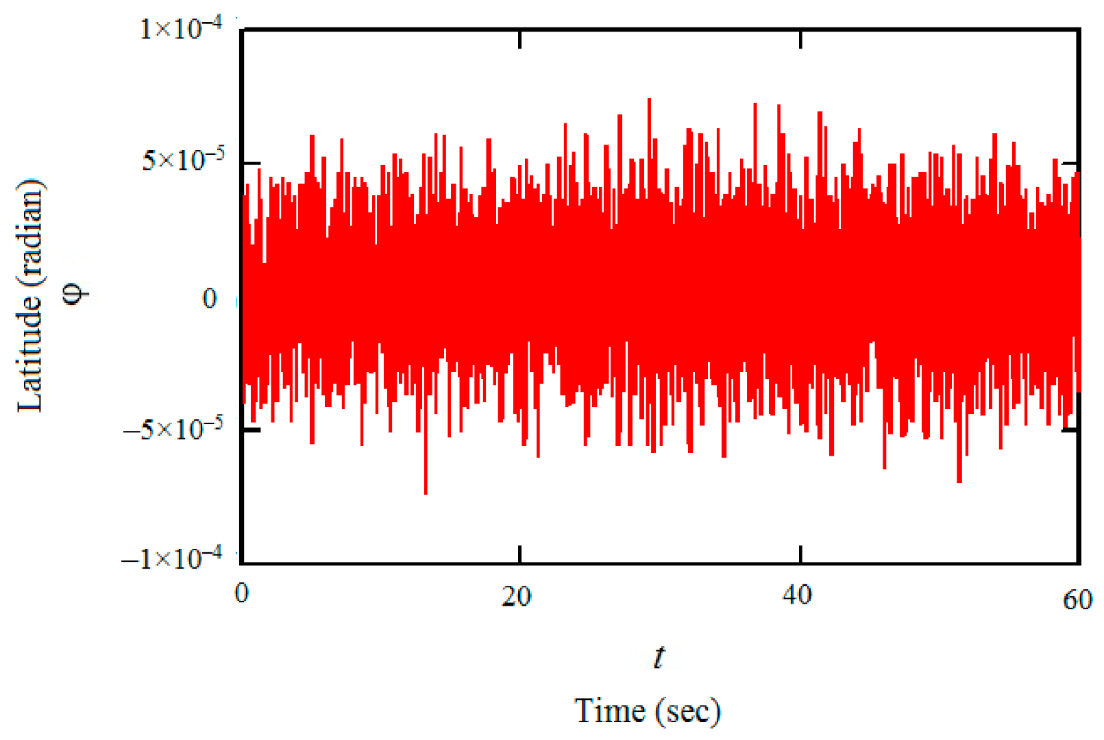
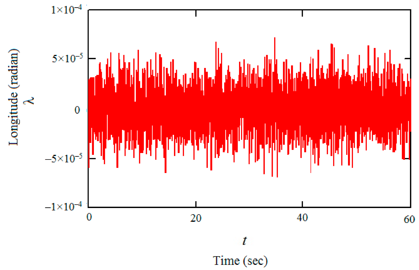
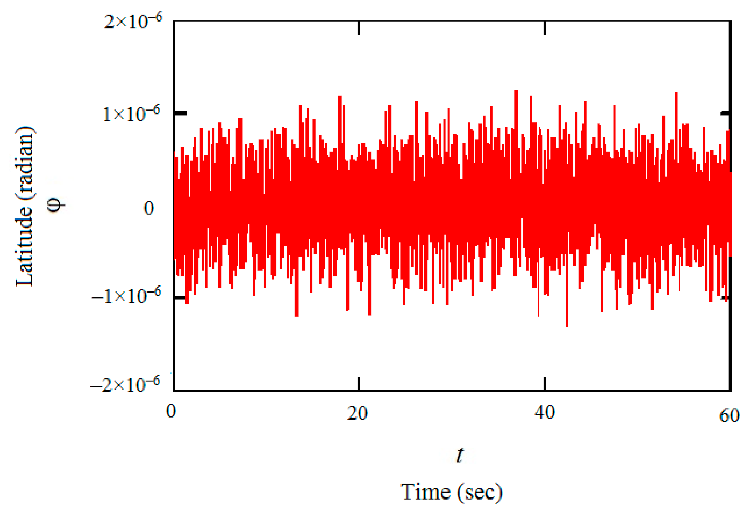
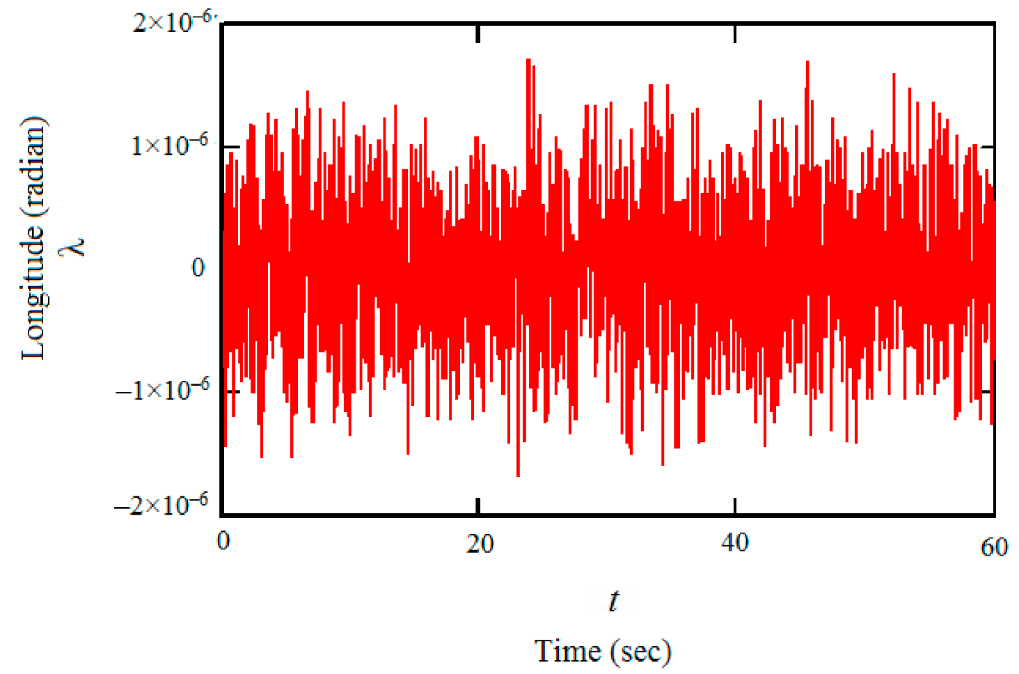
In the more general case of forming a measurement vector—when the interference of its components is mutually correlated, the covariance matrix R_K may be non-diagonal, which somewhat complicates the procedure for its calculation. First, with the dimension of the state vector N, the dimension of the matrix R_K is generally equal to N², which requires additional accurate measurements at N time steps. In practice, this possibility is often quite feasible—on roads and railways with a developed system of various road landmarks, in inertial satellite navigation systems with a high frequency (up to 100 Hz) transmission of satellite messages, etc.

Secondly, in order to be able to analytically determine all the components of the matrix R_K, the obtained measurements must be regrouped accordingly, followed by the solution of a new system of equations. In this case, the algorithm construction scheme takes the following form.

The exact measurements obtained at N time steps transform the estimation scheme as follows:

$$\begin{gathered} X_{\mathrm{k}}={\Phi }_{\mathrm{k}}{\widehat{X}}_{\mathrm{k}-1}+K_{\mathrm{k}}\left(Z_{\mathrm{k}}-H_{\mathrm{k}}{\Phi }_{\mathrm{k}}{\widehat{X}}_{\mathrm{k}-1}\right), \\ {X}_{\mathrm{k}+1}={\Phi }_{\mathrm{k}+1}{X}_{\mathrm{k}+1}+K_{\mathrm{k}+1}\left(Z_{\mathrm{k}+1}-H_{\mathrm{k}+1}{\Phi }_{\mathrm{k}}{X}_{\mathrm{k}}\right), \\ {X}_{\mathrm{k}+2}={\Phi }_{\mathrm{k}+2}{X}_{\mathrm{k}+1}+K_{\mathrm{k}+2}\left(Z_{\mathrm{k}+2}-H_{\mathrm{k}+2}{\Phi }_{\mathrm{k}}{X}_{\mathrm{k}+1}\right), \\ ⋮ \\ {X}_{\mathrm{k}+\mathrm{N}-1}={\Phi }_{\mathrm{k}+\mathrm{N}-1}{X}_{\mathrm{k}+\mathrm{N}-2}+K_{\mathrm{k}+\mathrm{N}-1}\left(Z_{\mathrm{k}+\mathrm{N}-1}-H_{\mathrm{k}+\mathrm{N}-1}{\Phi }_{\mathrm{k}}{X}_{\mathrm{k}+\mathrm{N}-2}\right). \end{gathered}$$

(9)

For each i-th step of the evaluation, transformations similar to Equations (5)–(7) are performed, after which the Eq’s system (9) is transformed into the system

$$\begin{gathered} U_{*1}=R_{\mathrm{K}}\cdot {\mathit{\Delta }}_{*1}, \\ {U}_{*2}=R_{\mathrm{K}}\cdot {\mathit{\Delta }}_{*2}, \\ {U}_{*3}=\underset{⋮}{R_{\mathrm{K}}}\cdot {\mathit{\Delta }}_{*3}, \\ {U}_{*\mathrm{N}}=R_{\mathrm{K}}\cdot {\mathit{\Delta }}_{*\mathrm{N}} \end{gathered}$$

(10)

where the matrix R_K is assumed to be constant at all N time steps

$$\begin{gathered} X_{*1}=X_{*},U_{*1}=U_{*},{\mathit{\Delta }}_{*1}={\mathit{\Delta }}_{*}, \\ {X}_{\mathrm{k}+\mathrm{i}}-{\Phi }_{\mathrm{k}+\mathrm{i}-1}{X}_{\mathrm{k}+\mathrm{i}-1}=X_{*\mathrm{i}},{\gamma }_{\mathrm{k}+\mathrm{i}}^{+}{\mathrm{X}}_{*\mathrm{i}}={\mathit{\Delta }}_{*\mathrm{i}}, \\ {Z}_{\mathrm{k}+\mathrm{i}}-H_{\mathrm{k}+\mathrm{i}}{\Phi }_{\mathrm{k}+\mathrm{i}}{X}_{\mathrm{k}+\mathrm{i}-1}=Z_{*\mathrm{i}},Z_{*\mathrm{i}}-H_{\mathrm{k}+\mathrm{i}}{X}_{*\mathrm{i}}=U_{*\mathrm{i}},\mathrm{i}=2,\dots ,\mathrm{N}. \end{gathered}$$

Next, the Equation (10) is transformed as follows: from each i-th subsystem of the equations $U_{*\mathrm{i}}=R_{\mathrm{K}}\cdot {\mathit{\Delta }}_{*\mathrm{i}}$ of dimension N, the j-th equation is selected, j = 1,...,N:

$$U_{*\mathrm{ij}}=R_{\mathrm{Kj}}\cdot {\mathit{\Delta }}_{*\mathrm{i}}$$

where $U_{*\mathrm{ij}}$ is the j-th component of the vector $U_{*\mathrm{i}}$, $R_{\mathrm{Kj}}$ is the j-th row of the matrix R_K. After that, a system of N linear equations is formed to determine all N components of the j-th row of the matrix R_K:

$$\begin{gathered} U_{*1\mathrm{j}}=R_{\mathrm{Kj}}\cdot {\mathit{\Delta }}_{*1}, \\ {U}_{*2\mathrm{j}}=R_{\mathrm{Kj}}\cdot {\mathit{\Delta }}_{*2}, \\ {U}_{*3\mathrm{j}}=R_{\mathrm{Kj}}\cdot {\mathit{\Delta }}_{*3}, \\ ⋮ \\ {U}_{*\mathrm{Nj}}=R_{\mathrm{Kj}}\cdot {\mathit{\Delta }}_{*\mathrm{N}} \end{gathered}$$

(11)

In vector form, the Eq’s system (11) can be written as

$$U_{*}^{\left(\mathrm{j}\right)}=\left|\begin{array}{l}{U}_{*1\mathrm{j}}\\ U_{*2\mathrm{j}}\\ U_{*3\mathrm{j}}\\ ⋮\\ U_{*\mathrm{Nj}}\end{array}\right|=\left|\begin{array}{l}{\mathit{\Delta }}_{*1}^{\mathrm{T}}\\ {\mathit{\Delta }}_{*2}^{\mathrm{T}}\\ {\mathit{\Delta }}_{*3}^{\mathrm{T}}\\ ⋮\\ {\mathit{\Delta }}_{*\mathrm{N}}^{\mathrm{T}}\end{array}\right|R_{\mathrm{Kj}}^{\mathrm{T}}$$

from where the j-th row of the matrix R_K is immediately determined

$${[U_{*}^{\left(\mathrm{j}\right)}]}^{\mathrm{T}}{\left|{\mathit{\Delta }}_{*1}{\mathit{\Delta }}_{*2}{\mathit{\Delta }}_{*3}\cdots {\mathit{\Delta }}_{*\mathrm{N}}\right|}^{-1}=R_{\mathrm{Kj}}$$

and, accordingly, the matrix R_K is

$$\left|\begin{array}{l}{[U_{*}^{\left(1\right)}]}^{\mathrm{T}}\\ {[U_{*}^{\left(2\right)}]}^{\mathrm{T}}\\ ⋮\\ {[U_{*}^{\left(\mathrm{N}\right)}]}^{\mathrm{T}}\end{array}\right|{\left|{\mathit{\Delta }}_{*1}{\mathit{\Delta }}_{*2}{\mathit{\Delta }}_{*3}\cdots {\mathit{\Delta }}_{*\mathrm{N}}\right|}^{-1}=R_{\mathrm{K}}$$

Here, as before, the task of adapting the Kalman estimation algorithm based on accurate observations is solved analytically.

In conclusion, it should be noted that the property of symmetry of the matrix R_K inherent in it by definition, on the one hand, reduces the number of its unknown components from N² to $\frac{{\mathrm{N}}^2+\mathrm{N}}{2}$, but, on the other hand, when solving (N − 1) systems of equations reduced with respect to Equation (11), requires the definition of (N − 1) inverse matrices, although reduced with respect to the matrix ${\left|{\mathit{\Delta }}_{*1}{\mathit{\Delta }}_{*2}{\mathit{\Delta }}_{*3}\cdots {\mathit{\Delta }}_{*\mathrm{N}}\right|}^{-1}=\Lambda$, but, nevertheless, requiring significant computational costs compared to a single calculation $\Lambda$. This circumstance allows us to consider the algorithm described above as the most efficient in terms of computational costs.

Next, consider an example that illustrates the effectiveness of the proposed approach.

3.3. Example

The movement of any object in the geographical coordinate system (GCS) is described by the following equation [45]:

$$\begin{gathered} \dot{\phi }=\frac{V_{\mathrm{y}}}{\left(r+h\right)}, \\ \dot{\lambda }=\frac{V_{\mathrm{x}}}{\cos \varphi \left(r+h\right)} \end{gathered}$$

(12)

where $\varphi ,\lambda$—the object’s latitude and longitude accordingly; r is the radius of the Earth; h is the object height; V_y, V_x are the linear velocity projections on the GCS-axes.

Next, we consider that the beginning coordinates of the object’s trajectory are defined as φ₀ = 0.8 rad, λ₀ = 0.3 rad, time interval of movement (0; 1000) s; the object moves at a constant velocity V = 20 m s⁻¹ along a loxodromic trajectory with an azimuthal angle at a constant speed along a loxodromic trajectory with an azimuthal angle A = 0.2 rad. In the process of movement, the topography of the Earth’s surface leads to a random change in the height of the object with zero expectation and standard deviation of 0.15 m. Based on the nature of the object’s trajectory, the projections of its linear velocity on the GSC-axes can be determined as follows:

$$\begin{gathered} V_{\mathrm{x}}=V\cdot \sin A, \\ {V}_{\mathrm{y}}=V\cdot \cos A \end{gathered}$$

We further assume that the navigation system (NS) of the object is built on the basis of weak integration of inertial NS (INS) and satellite NS (SNS). The measurement complex of this integrated NS receives satellite measurements at intervals of 20, 15 and 30 s, which are considered accurate. At other times, to estimate the vector of navigation parameters with a clock cycle of 0.1 s, INS measurements are used for channels λ and φ, for which the CMMN has the $R_{\mathrm{k}}=\left|\begin{array}{c}4,2\cdot {10}^{-10} 0 \\ 0 9,5\cdot {10}^{-10}\end{array}\right|$ (rad)².

Due to the fact that the speed of movement of an object causes a slight change in its coordinates at a given time interval, it is possible to use linearized navigation equations Equation (12) [45] relative to the initial coordinates for the subsequent solution of the problem

$$\begin{gathered} \dot{\phi }\left(\mathrm{t}\right)=\frac{V_{\mathrm{y}}\cdot \left(r+2h_0\right)}{(r+h_0){\cos }^2}-\frac{V_{\mathrm{y}}}{{(r+h_0)}^2}\cdot h, \\ \dot{\lambda }\left(\mathrm{t}\right)=\frac{V_{\mathrm{x}}}{\cos {\phi }_0\cdot \left(r+h_0\right)}\cdot \left[\frac{r+2h_0}{r+h_0}-\frac{\sin {\phi }_0\cdot {\phi }_0}{\cos {\phi }_0}\right]-\frac{V_{\mathrm{x}}}{\cos {\phi }_0\cdot {(r+h_0)}^2}\cdot h+\frac{V_{\mathrm{x}}\cdot \sin {\phi }_0}{{\cos }^2{\phi }_0\cdot \left(r+h_0\right)}\cdot \phi \end{gathered}$$

(13)

Since, in accordance with the example conditions, the change in the object height is a random process with zero expectation and a standard deviation of 0.15 m, then we assume h₀ = 0. Reducing the Equation (13) to a discrete form by the Eulers method with a sampling step τ:

$$\begin{gathered} {\phi }_k={\phi }_{k-1}+\tau \frac{V_y}{r}-\tau \frac{V_y}{r^2}\cdot h_k, \\ {\lambda }_{\mathrm{k}}={\lambda }_{\mathrm{k}-1}+\tau \frac{V_{\mathrm{x}}\cdot \tan {\phi }_0}{r\cos {\phi }_0}\cdot {\phi }_{\mathrm{k}-1}+\tau \frac{V_{\mathrm{x}}}{r\cos {\phi }_0}\cdot \left[1-{\phi }_0\tan {\phi }_0\right]-\tau \frac{V_{\mathrm{x}}}{\cos {\phi }_0\cdot r^2}\cdot h_{\mathrm{k}} \end{gathered}$$

we have a filter that in the accepted notation has the form:

$${\widehat{X}}_{\mathrm{k}+1}={\Phi }_{\mathrm{k}}{\widehat{X}}_{\mathrm{k}}+{\Omega }_{\mathrm{k}}+K_{\mathrm{k}}\left(Z_{\mathrm{k}}-H_{\mathrm{k}}{\Phi }_{\mathrm{k}}{\widehat{X}}_{\mathrm{k}}\right)$$

(14)

where

$$\begin{gathered} {\widehat{X}}_{\mathrm{k}}=\left|\begin{array}{c}\widehat{\phi }\\ \widehat{\lambda }\end{array}\right|, \\ {\Phi }_{\mathrm{k}}=\left|\begin{array}{l}10\\ \tau \frac{V_{\mathrm{x}}\tan {\phi }_0}{r\cos {\phi }_0}1\end{array}\right|, \\ {\Omega }_{\mathrm{k}}=\left|\begin{array}{l}\tau \frac{V_{\mathrm{y}}}{r}\\ \tau \frac{V_{\mathrm{x}}}{r\cos {\phi }_0}\left(1-{\phi }_0\mathrm{tg}{\phi }_0\right)\end{array}\right|, \\ {Q}_{\mathrm{k}}=\left|\begin{array}{l}{(\tau \frac{V_{\mathrm{y}}}{r^2}\cdot 0.15)}^2\frac{V_{\mathrm{y}}}{r^2}\cdot \frac{V_{\mathrm{x}}}{r^2\cos {\phi }_0}\cdot {(\tau \cdot 0.15)}^2\\ \frac{V_{\mathrm{y}}}{r^2}\cdot \frac{V_{\mathrm{x}}}{r^2\cos {\phi }_0}\cdot {(\tau \cdot 0.15)}^2{(\tau \frac{V_{\mathrm{x}}}{r^2\cos {\phi }_0}\cdot 0.15)}^2\end{array}\right|, \\ {H}_{\mathrm{k}}=\left|\begin{array}{cc}1& 0\\ 0& 1\end{array}\begin{array}{c}\\ \end{array}\right| \end{gathered}$$

Since the CMMN R_k is unknown under the initial conditions, the estimation of navigation variables was conducted for two cases: when the value of R_k is set with an error over the entire modeling interval $R_{\mathrm{k}}=\left|\begin{array}{c}1,1\cdot {10}^{-10} 0\\ 0 2,5\cdot {10}^{-10}\end{array}\right|$ (rad)², and when the R_k value is estimated according to the proposed algorithm.

Graphs of estimation errors obtained when implementing the Equation (14) in the first version are shown in Figure 1 and Figure 2, where a significant error in the estimation of the current coordinates of the object is obvious: the latitude error lies in the range from 100 to 350 m, the longitude from 50 to 200 m.

Figure 1. Graph of errors in estimating the latitude φ of the object obtained by implementing the classical Kalman filter.

Figure 2. Graph of errors in estimating the longitude λ of the object obtained by implementing the classical Kalman filter.

When designing an adaptive filter in accordance with the above algorithm, the estimation errors have the form shown in Figure 3 and Figure 4.

Figure 3. Graph of errors in estimating the latitude φ of the object obtained by implementing the adaptive filter.

Figure 4. Graph of errors in estimating the longitude λ of the object obtained by implementing the adaptive filter.

It is obvious that when using the proposed algorithm, the estimation errors in comparison with the traditional scheme changed sharply to the range from 2 to 7 m in latitude, and from 1.5 to 4 m in longitude.

For a more complete assessment of the capabilities of the proposed approach, it was compared with the innovation-based adaptive estimation algorithm [47] with the same model parameters and errors in setting the CMMN. When using innovation-based adaptive estimation, the covariance matrix R_k was evaluated in accordance with the equation [47]

$${\widehat{R}}_{\mathrm{k}}=\frac{1}{N}{\displaystyle \sum }_{\mathrm{j}={\mathrm{j}}_0}^{\mathrm{k}}{\upsilon }_{\mathrm{j}}{\upsilon }_{\mathrm{j}}{}^{\mathrm{T}}-H_{\mathrm{k}}{P}_{\mathrm{k}/\mathrm{k}-1}{H}_{\mathrm{k}}{}^{\mathrm{T}}$$

where ${\upsilon }_{\mathrm{k}}=Z_{\mathrm{k}}-{\widehat{Z}}_{\mathrm{k}/\mathrm{k}-1}$ is the discrepancy between the received measurement and its predicted value;

• N is the number of samples in the sliding “window” of the measurement in which the covariance matrix $R_{\mathrm{k}}$ is estimated;
• j₀ = k − N + 1 is the initial position of the sliding “window“.

In the case under study, N was chosen to be 25, and the sliding window was used three times for the 50th, 250th, and 800th seconds. The character of changes in estimation errors for both coordinates remained the same as in the developed algorithm, but the estimation errors themselves increased significantly in comparison to the range from 20 to 37 m in latitude and from 15 to 28 m in longitude.

4. Conclusions

A comparison of all the considered variants of traditional and adaptive filtration clearly shows the advantages of the proposed algorithm, despite the slight increase in computational cost (very small relative to total costs for a traditional filter; the Central Processing Unit (CPU) operation time for the combined calculation of the covariance matrix estimation and the current step of the filtration equation (14) was 1.849 s, and without the calculation of the covariance matrix estimation was 1.253 s). The simplicity, stability, convergence, and accuracy of the proposed algorithm make it possible to effectively use it for a wide range of measurements: measurements of motion parameters of unmanned objects, assessment of spacecraft orientation, measurements of chemical process characteristics, measurements of state parameters of complex mechanical systems, and others.

References

- Kurtz, V.; Lin, H. Kalman Filtering with Gaussian Processes Measurement Noise. 2019. preprint. [Google Scholar]
- Yeo, K.; Melnyk, I. Deep learning algorithm for data-driven simulation of noisy dynamical system. J. Comput. Phys. 2019, 376, 1212–1231. [Google Scholar] [CrossRef]
- Ohsumi, A.; Nakano, N. Identification of physical parameters of a flexible structure from noisy measurement data. IEEE Trans. Instrum. Meas. 2002, 51, 923–929. [Google Scholar] [CrossRef]
- Khan, N.; Jabbar, A.; Bilal, H.; Gul, U. Compensated closed-loop Kalman filtering for nonlinear systems. Measurement 2020, 151, 107129. [Google Scholar] [CrossRef]
- Rodriguez-Maldonado, J. Estimation of angular velocity and acceleration with Kalman filter, based on position measurement only. Measurement 2019, 145, 130–136. [Google Scholar] [CrossRef]
- Xu, C.; Huang, D.; Liu, J. Target location of unmanned aerial vehicles based on the electro-optical stabilization and tracking platform. Measurement 2019, 147, 106848. [Google Scholar] [CrossRef]
- Wang, D.; Dong, Y.; Li, Q.; Wu, J.; Wen, Y. Estimation of small UAV position and attitude with reliable in-flight initial alignment for MEMS inertial sensors. Metrol. Meas. Syst. 2018, 25, 603–616. [Google Scholar]
- Qu, Y.; Yan, J.; Pan, Q.; Fan, C. Study on the filtering method of the navigation data of a UAV. In Proceedings of the ISTM/2005: 6th International Symposium on Test and Measurement; Wen, T., Ed.; International Academic Publishers: Dalian, China, 2005; pp. 7684–7687. [Google Scholar]
- Wang, D.; Lv, H.; Wu, J. Augmented Cubature Kalman filter for nonlinear RTK/MIMU integrated navigation with non-additive noise. Measurement 2017, 97, 111–125. [Google Scholar] [CrossRef]
- Salehi, Y.; Fatehi, A.; Nayebi, M.A. State Estimation of Slow-Rate Integrated Measurement Systems in the Presence of Parametric Uncertainties. IEEE Trans. Instrum. Meas. 2019, 68, 3983–3991. [Google Scholar] [CrossRef]
- Kaniewski, P.; Gil, R.; Konatowski, S. Estimation of UAV Position with Use of Smoothing Algorithms. Metrol. Meas. Syst. 2017, 24, 127–142. [Google Scholar] [CrossRef]
- Xu, X.; Xu, X.; Zhang, T.; Wang, Z. In-Motion Filter-QUEST Alignment for Strapdown Inertial Navigation Systems. IEEE Trans. Instrum. Meas. 2018, 67, 1979–1993. [Google Scholar] [CrossRef]
- Meng, Z.; Pan, Z.; Chen, Z.; Shi, Y. Adaptive signal fusion based on relative fluctuations of variable signals. Measurement 2019, 148, 106909. [Google Scholar] [CrossRef]
- Sinitsyn, I.N. Kalman and Pugachev filters [in Russian]; Logos: Moscow, Russia, 2007; ISBN 978-5-98704-270-4. [Google Scholar]
- Reif, K.; Unbehauen, R. The extended Kalman filter as an exponential observer for nonlinear systems. IEEE Trans. Signal Process. 1999, 47, 2324–2328. [Google Scholar] [CrossRef]
- Anderson, B.D.O. Exponential data weighting in the Kalman-Bucy filter. Inf. Sci. 1973, 5, 217–230. [Google Scholar] [CrossRef]
- Xiong, J. An Introduction to Stochastic Filtering Theory; Oxford University Press: New York, NY, USA, 2008; ISBN 978-0-19-921970-4. [Google Scholar]
- Senne, K. Stochastic processes and filtering theory. IEEE Trans. Automat. Contr. 1972, 17, 752–753. [Google Scholar] [CrossRef]
- Ferrero, A.; Ferrero, R.; Jiang, W.; Salicone, S. The Kalman Filter Uncertainty Concept in the Possibility Domain. IEEE Trans. Instrum. Meas. 2019, 68, 4335–4347. [Google Scholar] [CrossRef]
- Kalman, R.E. Mathematical Description of Linear Dynamical Systems. J. Soc. Ind. Appl. Math. Ser. A Control 1963, 1, 152–192. [Google Scholar] [CrossRef]
- Sokolov, S.V. Application of non-Gaussian distribution at the synthesis of suboptimal filtration algorithms. Izv. Vyss. Uchebnykh Zaved. Radioelektronika 1991, 34, 8–11. [Google Scholar]
- Sokolov, S.V.; Novikov, A.I. Adaptive estimation of UVs navigation parameters by irregular inertial-satellite measurements. Int. J. Intell. Unmanned Syst. 2020. In Press. [Google Scholar] [CrossRef]
- Sokolov, S.V.; Novikov, A.I.; Ivetić, V. Determining the initial orientation for navigation-measurement systems of mobile apparatus in reforestation. Inventions 2019, 4, 56. [Google Scholar] [CrossRef]
- De Mendonça, C.B.; Hemerly, E.M.; Góes, L.C.S. Adaptive Stochastic Filtering for Online Aircraft Flight Path Reconstruction. J. Aircr. 2007, 44, 1546–1558. [Google Scholar] [CrossRef]
- Lei, X.; Li, J. An adaptive navigation method for a small unmanned aerial rotorcraft under complex environment. Measurement 2013, 46, 4166–4171. [Google Scholar] [CrossRef]
- Kucherenko, P.A.; Sokolov, S.V. A solution of the problem of nonlinear parametric identification based on generalized probability criteria. J. Comput. Syst. Sci. Int. 2008, 47, 703–708. [Google Scholar] [CrossRef]
- Sokolov, S.; Marshakov, D.; Novikov, A. The current spectrum formation of a non-periodic signal: A differential approach. Inventions 2020, 5, 15. [Google Scholar] [CrossRef]
- Sasiadek, J.Z.; Wang, Q. Low cost automation using INS/GPS data fusion for accurate positioning. Robotica 2003, 21, 255–260. [Google Scholar] [CrossRef]
- Herrera, E.P.; Kaufmann, H. Adaptive methods of Kalman filtering for personal positioning systems. In Proceedings of the 23rd International Technical Meeting of the Satellite Division of the Institute of Navigation 2010 (ION GNSS 2010), Portland, Oregon, 21–24 September 2010. [Google Scholar]
- Hide, C.; Moore, T.; Smith, M. Adaptive Kalman filtering algorithms for integrating GPS and low cost INS. In Proceedings of the PLANS 2004. Position Location and Navigation Symposium (IEEE Cat. No.04CH37556), Monterey, CA, USA, 26–29 April 2004; pp. 227–233. [Google Scholar]
- Hu, C.; Chen, W.; Chen, Y.; Liu, D. Adaptive Kalman Filtering for Vehicle Navigation. J. Glob. Position. Syst. 2003, 2, 42–47. [Google Scholar] [CrossRef]
- Mehra, R. On the identification of variances and adaptive Kalman filtering. IEEE Trans. Automat. Contr. 1970, 15, 175–184. [Google Scholar] [CrossRef]
- Mohamed, A.H.; Schwarz, K.P. Adaptive Kalman filtering for INS/GPS. J. Geod. 1999, 73, 193–203. [Google Scholar] [CrossRef]
- Qiu, Z.; Huang, Y.; Qian, H. Adaptive Robust Nonlinear Filtering for Spacecraft Attitude Estimation Based on Additive Quaternion. IEEE Trans. Instrum. Meas. 2020, 69, 100–108. [Google Scholar] [CrossRef]
- Kim, D.; Min, K.; Kim, H.; Huh, K. Vehicle sideslip angle estimation using deep ensemble-based adaptive Kalman filter. Mech. Syst. Signal Process. 2020, 144, 106862. [Google Scholar] [CrossRef]
- Ma, T.; Chen, C.; Gao, S. Model set adaptive filtering algorithm using variational Bayesian approximations and Rényi information divergence. EURASIP J. Adv. Signal Process. 2020, 2020, 17. [Google Scholar] [CrossRef]
- Miao, Z.; Shi, H.; Zhang, Y.; Xu, F. Neural network-aided variational Bayesian adaptive cubature Kalman filtering for nonlinear state estimation. Meas. Sci. Technol. 2017, 28, 105003. [Google Scholar] [CrossRef]
- Litvin, M.A.; Malyugina, A.A.; Miller, A.B.; Stepanov, A.N.; Chickrin, D.E. Error Classification and Approximation in Inertial Navigational Systems. Inf. Process. 2014, 14, 326–339. [Google Scholar]
- Reznichenko, V.I.; Maleev, P.I.; Smirnov, M.Y. The satellite correction of orientation parameters for marine objects. Navig. Hydrogr. 2008, 27, 25–32. [Google Scholar]
- Tsyplakov, A.A. An introduction to state space modelling. Quantile 2011, 5, 1–24. [Google Scholar]
- Novikov, A.I.; Ersson, B.T. Aerial seeding of forests in Russia: A selected literature analysis. IOP Conf. Ser. Earth Environ. Sci. 2019, 226, 012051. [Google Scholar] [CrossRef]
- Chen, C.; Chang, G. Low-cost GNSS/INS integration for enhanced land vehicle performance. Meas. Sci. Technol. 2020, 31, 035009. [Google Scholar] [CrossRef]
- Shilina, V.A. Inertial Sensor System for Indoor Navigation. Available online: http://ainsnt.ru/doc/778220.html (accessed on 5 January 2020).
- Sokolov, S.V.; Polyakova, M.V.; Kucherenko, P.A. Analytic Synthesis of a Kalman Adaptive Filter on the Basis of Irregular Precise Measurements. Meas. Tech. 2018, 61, 232–237. [Google Scholar] [CrossRef]
- Rozenberg, I.N.; Sokolov, S.V.; Umansky, V.I.; Pogorelov, V.A. The Theoretical Basis of the Tight Integration of Inertial-Satellite Navigation Systems; Fizmatlit: Moscow, Russia, 2018. [Google Scholar]
- Gantmakher, F.R. The Theory of Matrices; Fizmatlit: Moscow, Russia, 1959; ISBN 0821813765. [Google Scholar]
- Jwo, D.-J.; Chung, F.-C.; Weng, T.-P. Adaptive Kalman Filter for Navigation Sensor Fusion. In Sensor Fusion and its Applications; Sciyo: Shanghai, China, 2010; pp. 65–90. [Google Scholar]
Publisher’s Note: MDPI stays neutral with regard to jurisdictional claims in published maps and institutional affiliations. |
© 2021 by the authors. Licensee MDPI, Basel, Switzerland. This article is an open access article distributed under the terms and conditions of the Creative Commons Attribution (CC BY) license (http://creativecommons.org/licenses/by/4.0/).