The CaliPhoto Method

 ,
,
Abstract
1. Introduction
2. Materials and Methods
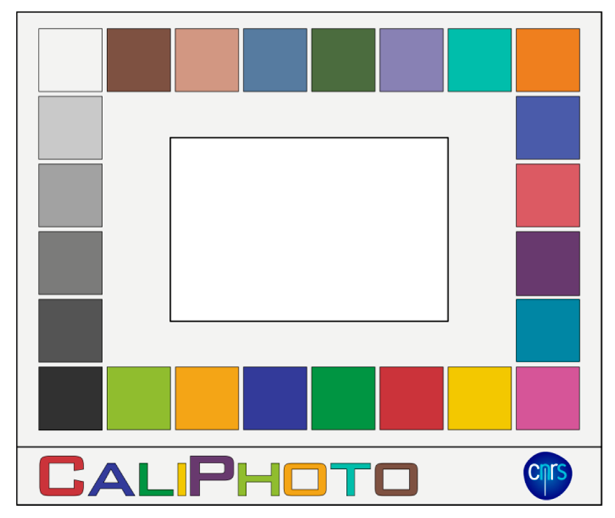
2.1. Printing the CaliPhoto Colour Plate
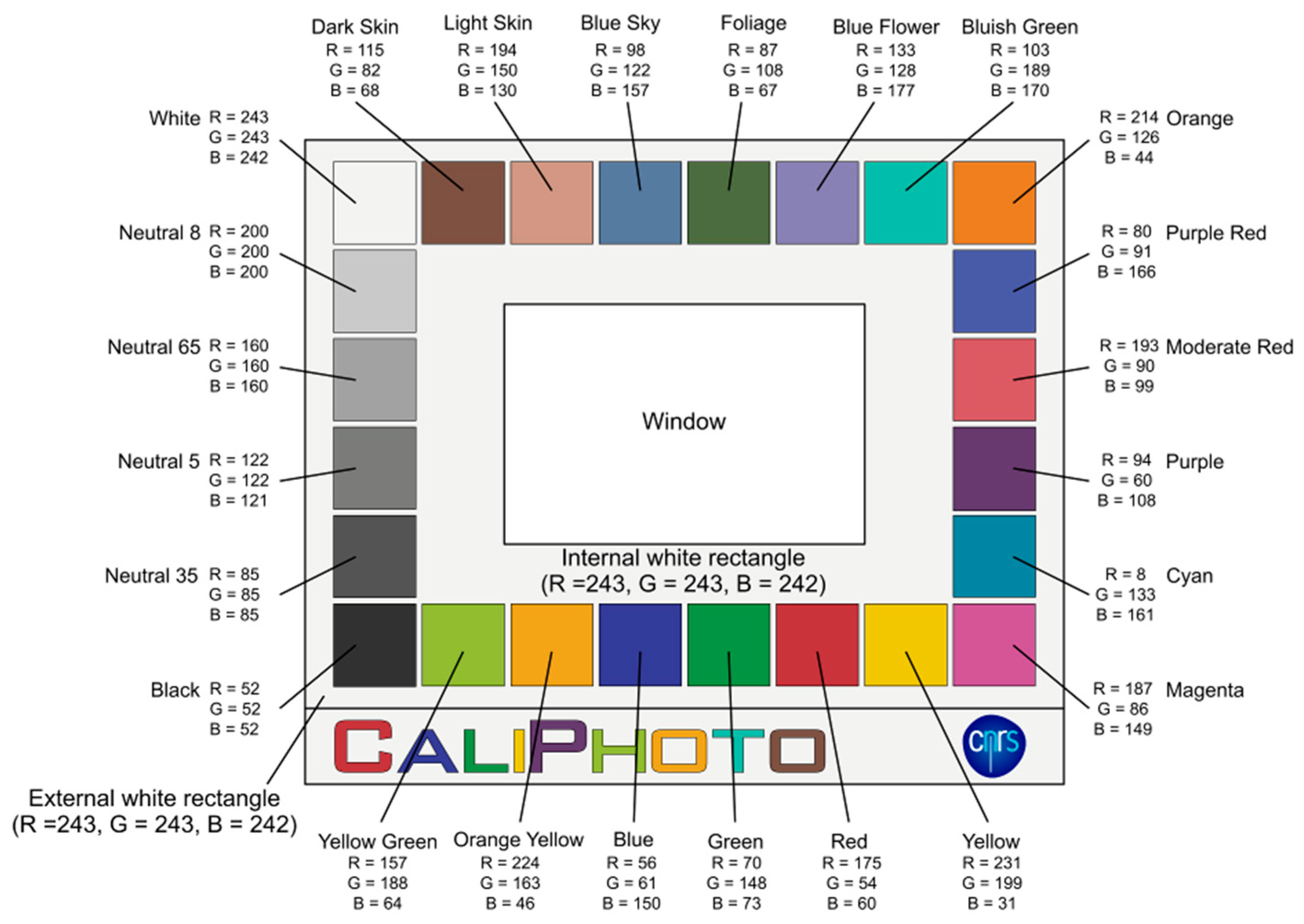
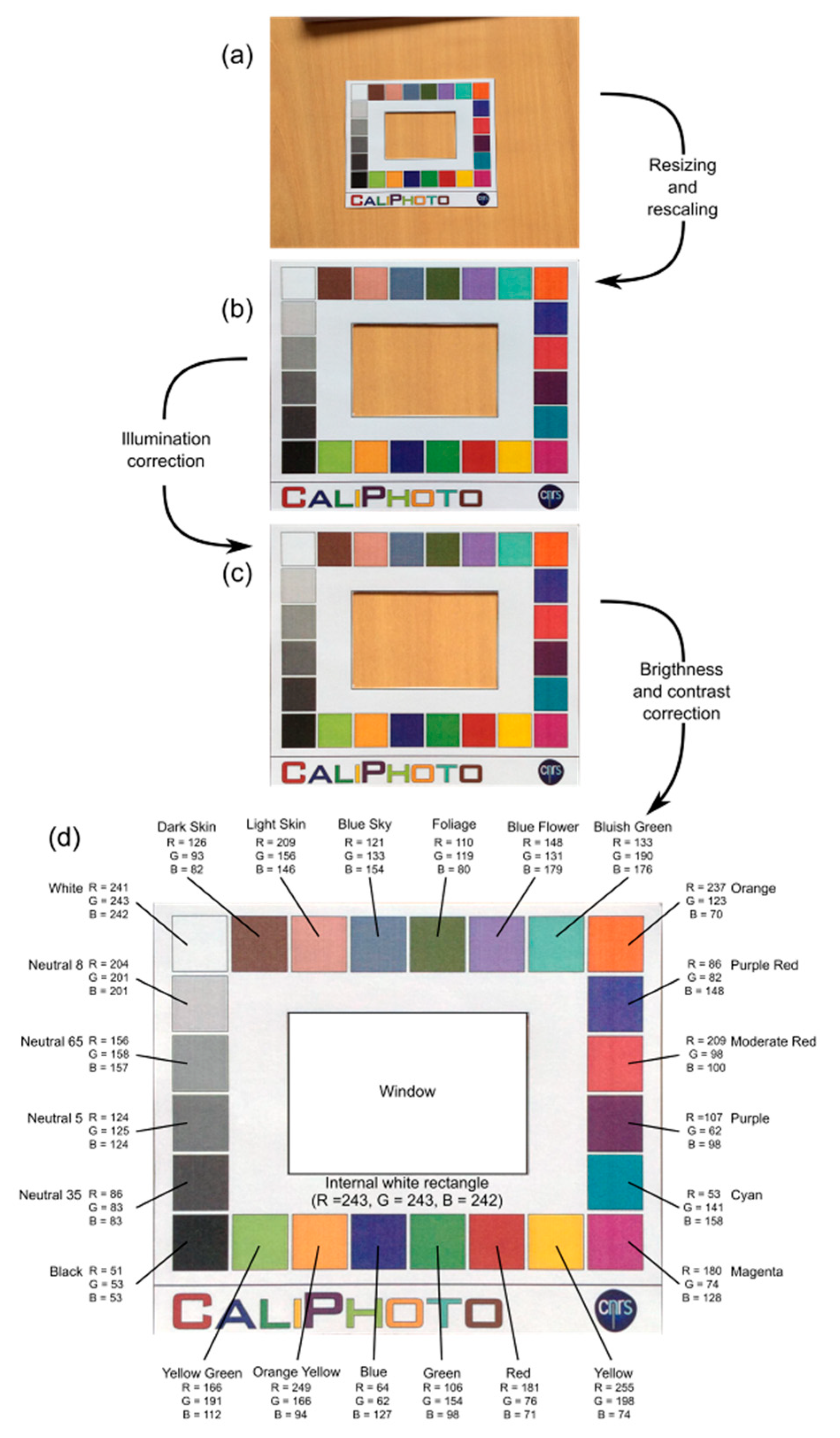
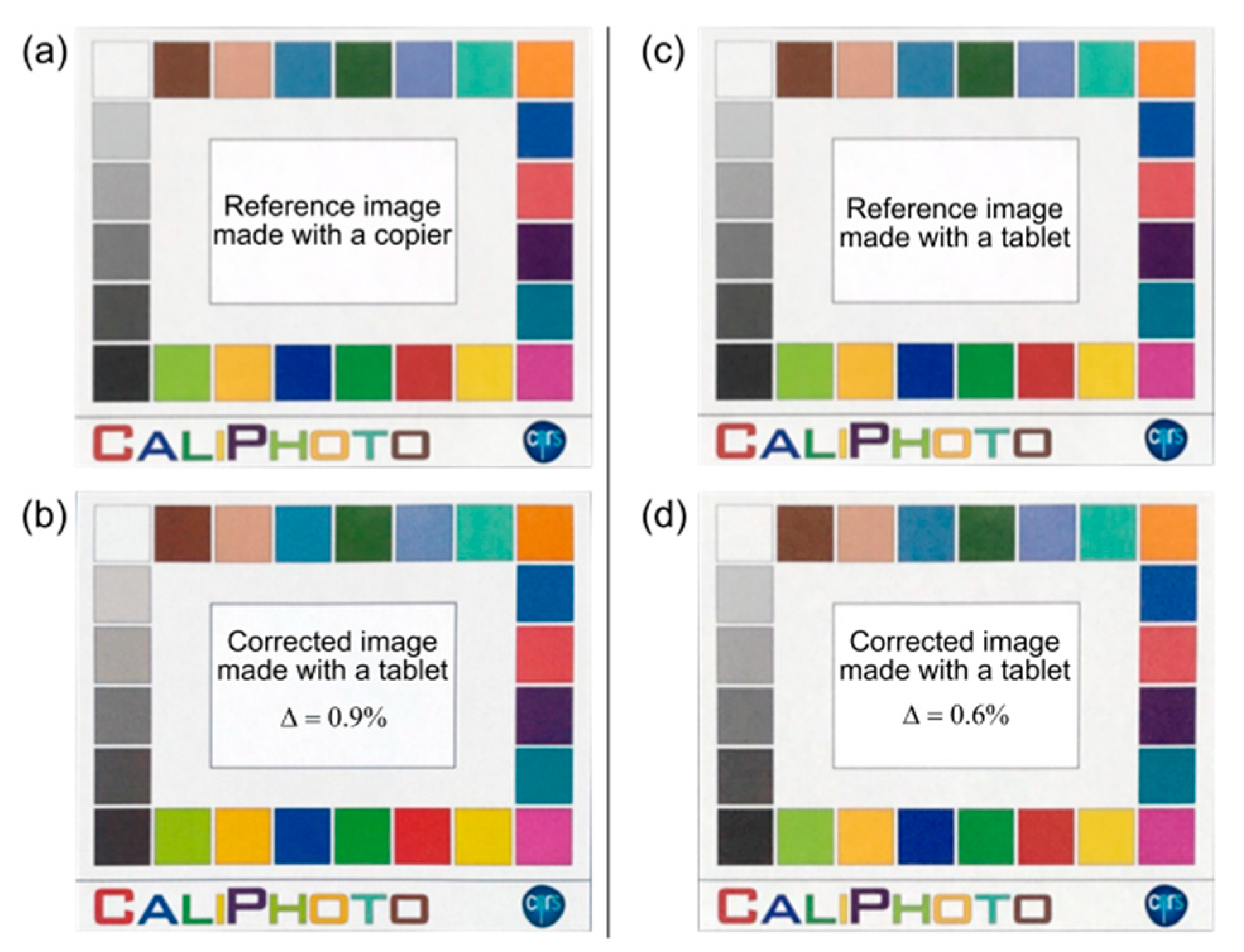
2.2. Make a Reference Image of the Printed CaliPhoto Colour Plate
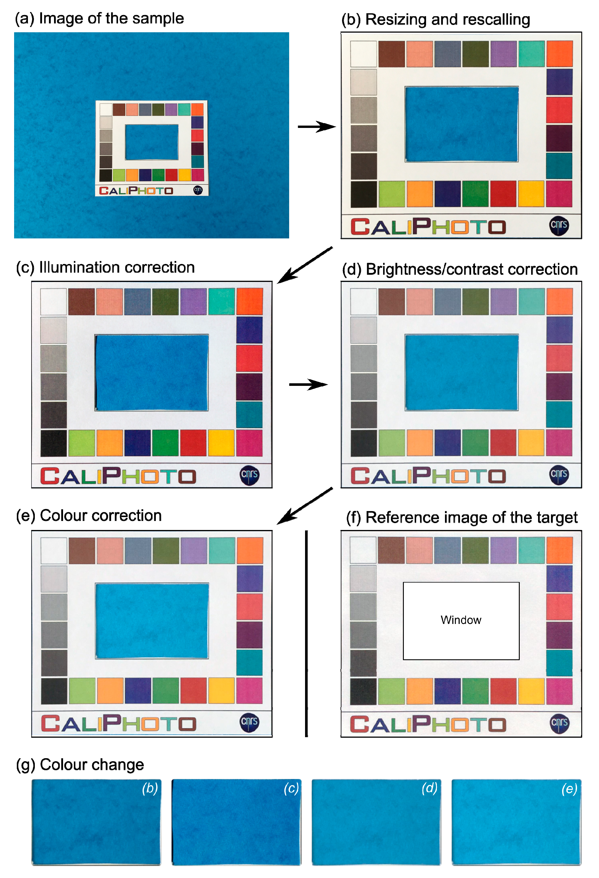
2.3. Making Comparable Images of the Materials
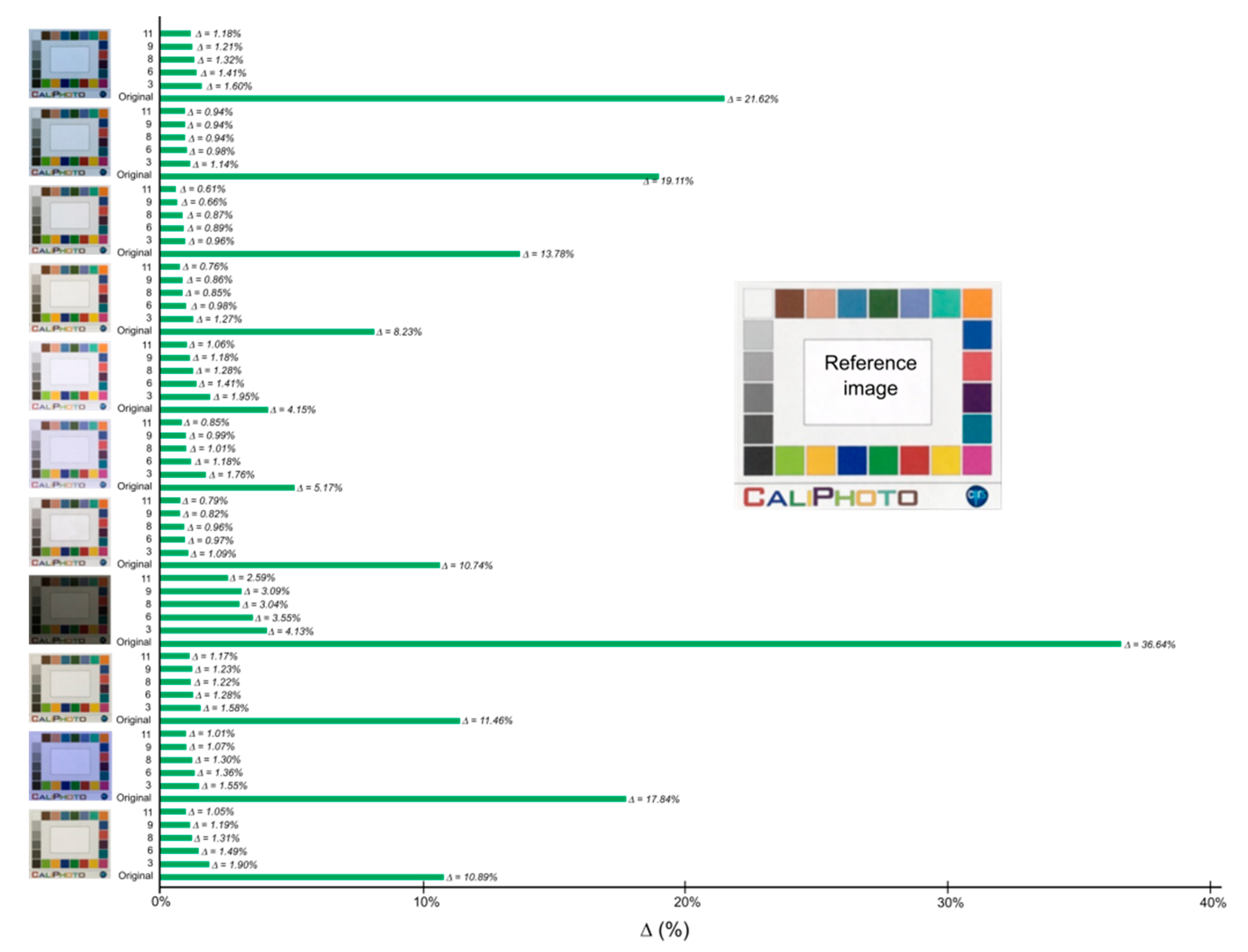
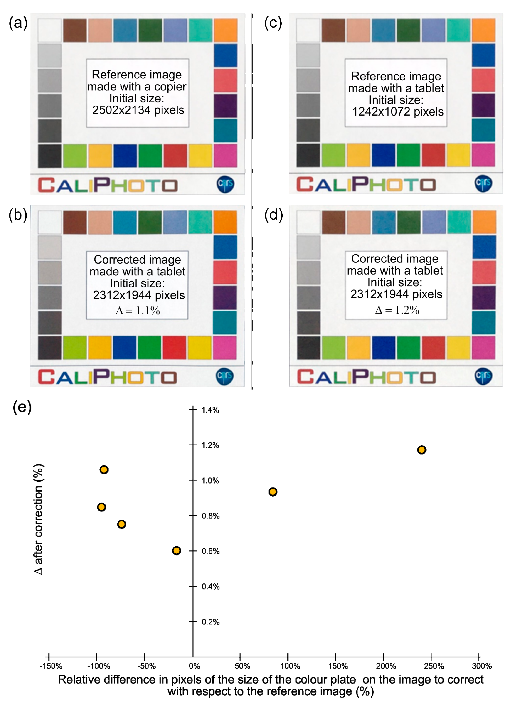
- The best correction is obtained when the size of the colour plate in pixels on the image is close to that of the colour plate on the reference image before resizing.
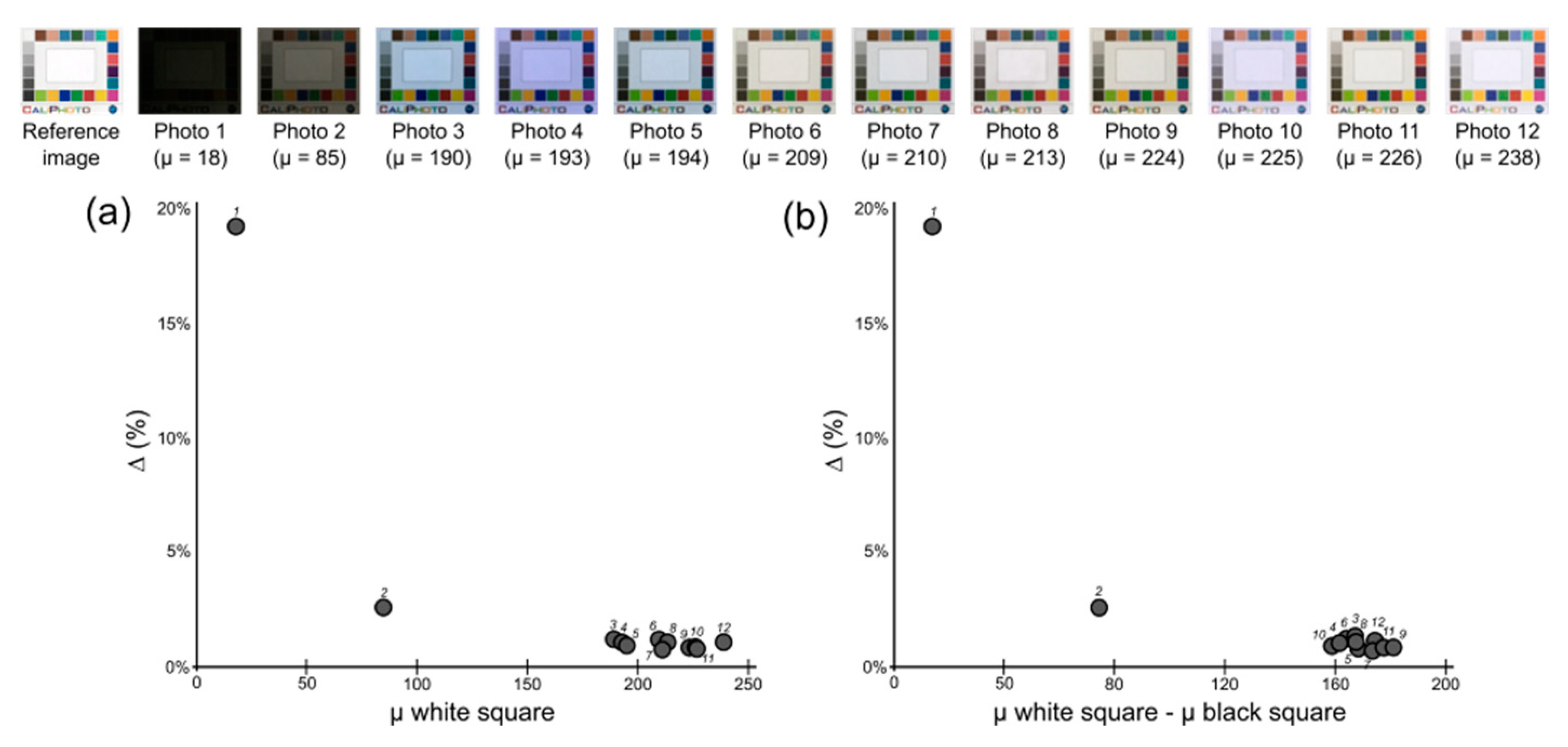
- The correction of an image with respect to the reference image remains good, even in low-light environments. It is shown that Δ < 3% when the luminance µ = (R + G + B)/3 of the white square in the sample image is higher than approximately 100, and when the image dynamic (i.e., µ of white square minus µ of black square) is higher than approximately 100.
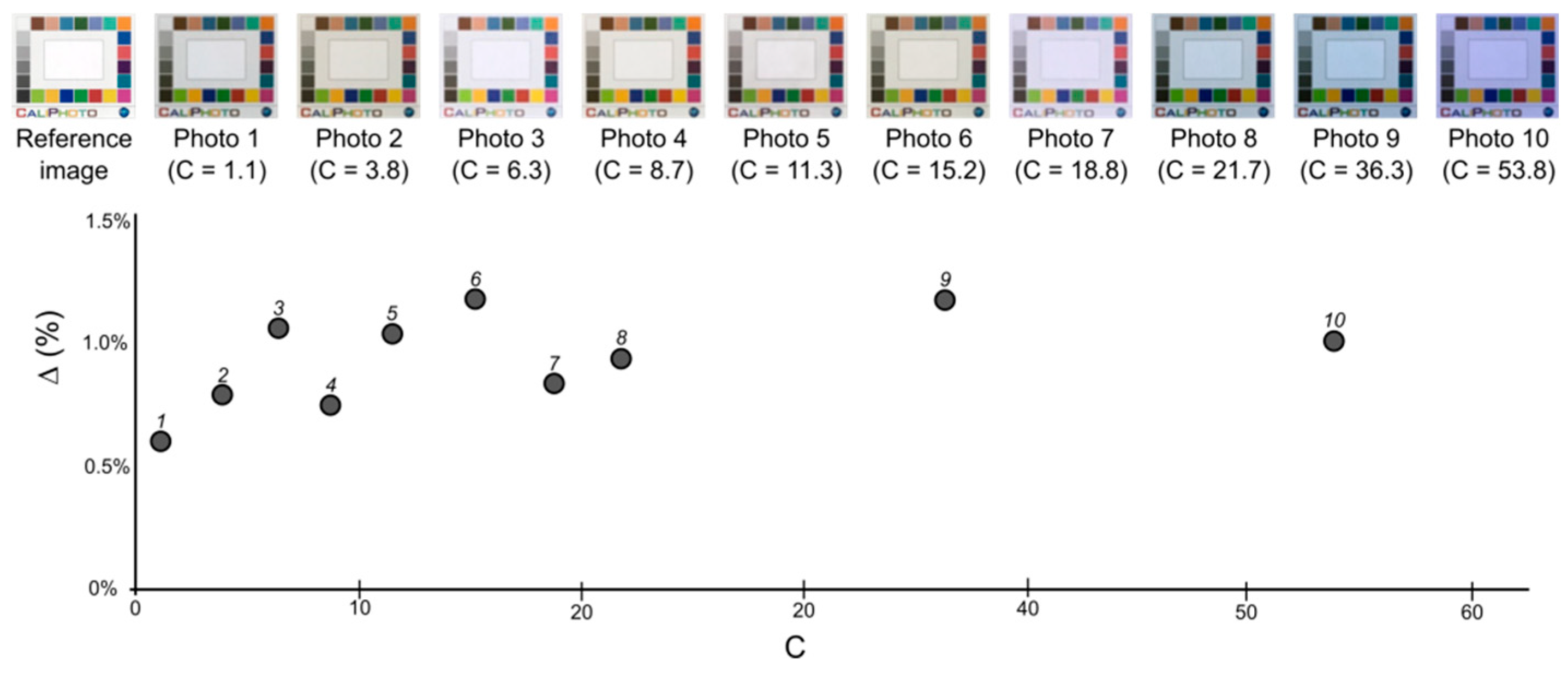
- The “colour” of the light does not play a role in the final correction; for a difference of 54 between the highest and the lowest of the three RGB values of the white square, Δ = 1%.
- It is better to use the same camera throughout the whole procedure, even if Δ < 2% when using different imaging devices.
2.4. Comparison of Materials from the Colours Given by CaliPhoto
3. Results
4. Discussion
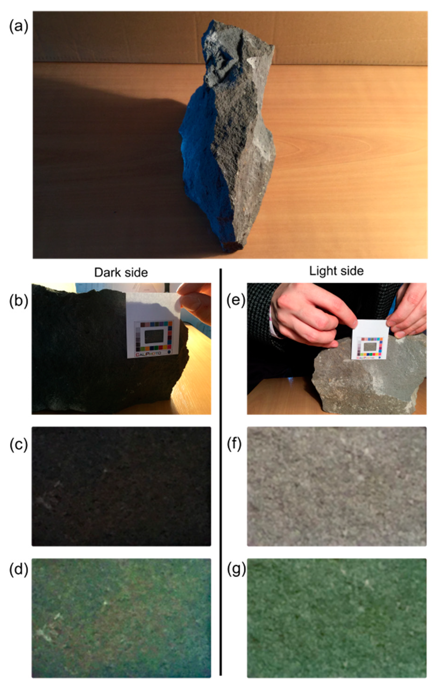
- Space exploration: As mentioned above, instrumentation used during in situ space exploration is generally limited for technical reasons (limited mass, volume, energy and computational power). On the other hand, all space probes have on board a camera. Integrating a CaliPhoto colour plate with imaging systems on future space probes would be simple since it easily complies with the imposed technical limitations and does not require the development of new instrumentation. It could be particularly relevant for geological and astrobiological investigations, permitting the comparison of images of rocks taken in different places or evaluation of lithologies using images of rocks taken in the laboratory, for example.
- Construction: The method may find different applications in this domain, for example, to check the homogeneity of materials over large areas or on the different faces of a structure, to monitor the ageing of materials over space and time, or to control the water content of cement.
- Geology: As for space exploration, the method allows easy comparison of samples observed in different places in the field. When associated with a database, it can also facilitate the use of soil colour charts.
- Biology: Colour is used as a parameter to pre-identify microbial colonies or to evaluate their reaction to external stresses (sunlight, dehydration, pH, salinity, etc.). This applies more generally for any living system (the yellowing of leaves, for example). The CaliPhoto may thus be used as a noninvasive and rapid method of monitoring such types of samples.
- Materials science: Changes in the physico-chemical characteristics of materials may be associated with a change in colour. The possibility to monitor such changes during specific experiments may be particularly useful in determining reaction kinetics. Association with a database linking specific properties to CaliPhoto colours may circumvent or limit the systematic use of sophisticated instrumentation. It may help to refine measurements based on colour, such as those obtained using pH paper.
- Submarine investigation: Underwater imaging is generally affected by water colour and inherently limited control of the light source. Submarine instrumentation is also limited compared with laboratory instrumentation. The CaliPhoto method may thus also be particularly useful in this setting. By linking physical properties obtained by laboratory analysis to a CaliPhoto database, it could be possible to estimate these properties from images made underwater, without sampling.
- Cosmetics and dermatology: The CaliPhoto method may assist in the selection of makeup adapted to specific types of skin. It may also provide a control for Sun exposure to prevent sunburn. In the latter case, the idea would be to take pictures regularly of the same part of the body to monitor any change in colour.
5. Patents
Supplementary Materials
Author Contributions
Funding
Conflicts of Interest
Appendix A. Print the CaliPhoto Colour Plate

Appendix B. Making the Reference Image of the Colour Plate


- (i).
- The rescaled and resized image (Figure A4a) is imported in MATLAB.
- (ii).
- The RGB channels of the image are extracted and converted into double format (Figure A4b).
- (iii).
- Pixels corresponding to the white rectangles surrounding the colour squares and the window on each of the three images are selected (see Figure A4c).
- (iv).
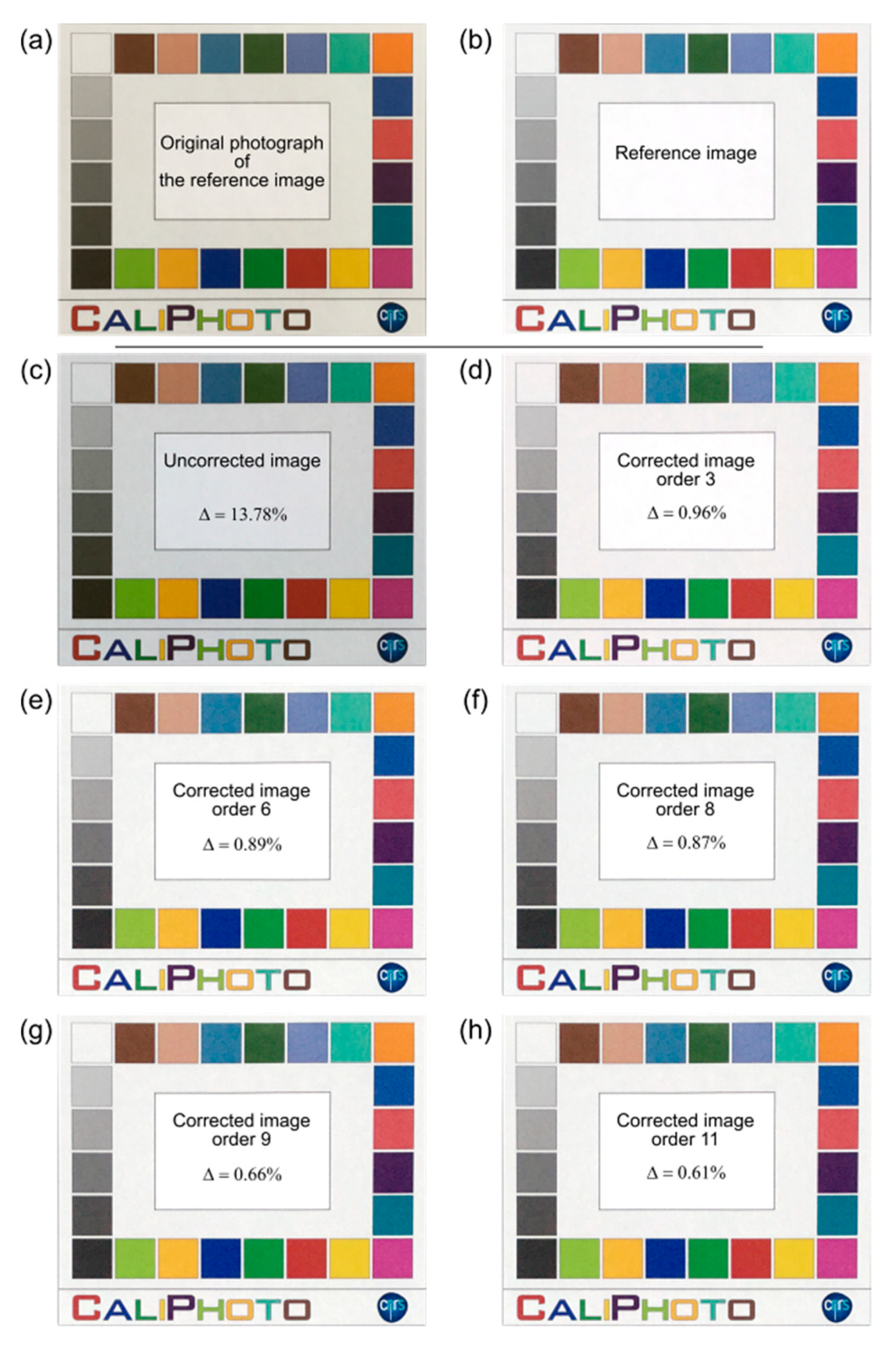
- The light source creates a homogeneous variation in brightness over the colour plate that can be fitted, for each R, G, B channel, by a polynomial plane equation (of order 3 in the example shown) determined from the two white rectangles selected in (iii) (Figure A4c).
- (v).
- The principle then becomes similar to the data processing method called “plane fit”, used in Scanning Probe Microscopy to correct the slope of the sample surface [11], consisting of removing the calculated plane from the whole image. In the CaliPhoto method, the plane removal is made in order to set the average value of the white rectangles to R,G,B = 230,230,230 (Figure A4d). The R,G,B values are set to 230,230,230 instead of 243,243,242 as expected in the final image to avoid values potentially higher than 255 after brightness and contrast adjustments made in the following step. This step also corrects the chromaticity of the illumination source by resetting the white balance. If the colour print is of lower quality (e.g., the white square appearing a more yellow in the printed colour plate), this step may also lead to apparent colours that are unattractive to human expectations in the processed image. However, it is important to note that, unlike colorimetric methods, this aspect of “unattractiveness” will not alter the accuracy of the method.
- (vi).
- The next step involves brightness and contrast correction. This is done by fitting the average value of the greyscale rectangles of the colour plate to their theoretical values, using a polynomial regression of order 3 (Figure A4e).
- (vii).
- Finally, it is possible to extract, as an Excel file for example, the average values of the colour squares of the reference image of the colour plate (Table A1).


| Theoretical Values | Reference Image of the Colour Plate | |||||
|---|---|---|---|---|---|---|
| Colour Plate Square | Rtheo | Gtheo | Btheo | Rref | Gref | Bref |
| Dark skin | 115 | 82 | 68 | 126 | 93 | 82 |
| Light skin | 194 | 150 | 130 | 209 | 156 | 146 |
| Blue sky | 98 | 122 | 157 | 121 | 133 | 154 |
| Foliage | 87 | 108 | 67 | 110 | 119 | 80 |
| Blue flower | 133 | 128 | 177 | 148 | 131 | 179 |
| Bluish green | 103 | 189 | 170 | 133 | 190 | 176 |
| Orange | 214 | 126 | 44 | 237 | 123 | 70 |
| Purple red | 80 | 91 | 166 | 86 | 82 | 148 |
| Moderate red | 193 | 90 | 99 | 209 | 98 | 100 |
| Purple | 94 | 60 | 108 | 107 | 62 | 98 |
| Cyan | 8 | 133 | 161 | 53 | 141 | 158 |
| Magenta | 187 | 86 | 149 | 180 | 74 | 128 |
| Yellow | 231 | 199 | 31 | 255 | 198 | 74 |
| Red | 175 | 54 | 60 | 181 | 76 | 71 |
| Green | 70 | 148 | 73 | 106 | 154 | 98 |
| Blue | 56 | 61 | 150 | 64 | 62 | 127 |
| Orange yellow | 224 | 163 | 46 | 249 | 166 | 94 |
| Yellow green | 157 | 188 | 64 | 166 | 191 | 112 |
| Black | 52 | 52 | 52 | 51 | 53 | 53 |
| Neutral 35 | 85 | 85 | 85 | 86 | 83 | 83 |
| Neutral 5 | 122 | 122 | 121 | 124 | 125 | 124 |
| Neutral 65 | 160 | 160 | 160 | 156 | 158 | 157 |
| Neutral 8 | 200 | 200 | 200 | 204 | 201 | 201 |
| White | 243 | 243 | 242 | 241 | 243 | 242 |
Appendix C. Making the CaliPhoto Image of the Material
Gfinal = b1R + b2G + b3B
Bfinal = c1R + c2G + c3B
Gfinal = b1R + b2G + b3B + b4R.G + b5G.B + b6R.B
Bfinal = c1R + c2G + c3B + c4R.G + c5G.B + c6R.B
Gfinal = b1R + b2G + b3B + b4R.G + b5G.B + b6R.B + b7R.B + b8R2 + b9G2 + b10B2 + b11R.G.B
Bfinal = c1R + c2G + c3B + c4R.G + c5G.B + c6R.B + c7R.B + c8R2 + c9G2 + c10B2 + c11R.G.B


| Reference Image of the Colour Plate | Initial Image Before Correction | Δ12(%) | Final Image After Correction | Δ12 (%) | |||||||
|---|---|---|---|---|---|---|---|---|---|---|---|
| Colour Plate Square | Rref | Gref | Bref | Rini | Gini | Bini | Rfinal | Gfinal | Bfinal | ||
| Dark skin | 112 | 75 | 59 | 78 | 56 | 33 | 10.67% | 111 | 75 | 58 | 0.39% |
| Light skin | 203 | 160 | 136 | 159 | 115 | 86 | 18.22% | 201 | 160 | 136 | 0.35% |
| Blue sky | 79 | 124 | 159 | 56 | 85 | 109 | 15.39% | 76 | 124 | 159 | 0.81% |
| Foliage | 66 | 96 | 58 | 54 | 70 | 33 | 8.52% | 66 | 97 | 59 | 0.44% |
| Blue flower | 120 | 134 | 180 | 81 | 93 | 132 | 16.80% | 122 | 136 | 181 | 0.66% |
| Bluish green | 107 | 184 | 159 | 75 | 140 | 108 | 16.87% | 103 | 181 | 158 | 1.11% |
| Orange | 229 | 146 | 62 | 189 | 107 | 36 | 13.90% | 225 | 146 | 63 | 0.98% |
| Purple red | 40 | 79 | 150 | 41 | 58 | 102 | 11.91% | 38 | 81 | 150 | 0.56% |
| Moderate red | 198 | 89 | 93 | 154 | 64 | 54 | 14.46% | 196 | 89 | 93 | 0.53% |
| Purple | 64 | 32 | 81 | 54 | 35 | 49 | 7.86% | 66 | 37 | 84 | 1.34% |
| Cyan | 1 | 110 | 135 | 22 | 79 | 89 | 13.51% | 2 | 111 | 135 | 0.39% |
| Magenta | 183 | 70 | 139 | 138 | 50 | 91 | 15.43% | 182 | 68 | 138 | 0.46% |
| Yellow | 232 | 202 | 65 | 195 | 163 | 31 | 14.50% | 231 | 202 | 65 | 0.30% |
| Red | 170 | 60 | 58 | 125 | 46 | 30 | 12.38% | 174 | 61 | 57 | 0.86% |
| Green | 68 | 143 | 69 | 49 | 101 | 35 | 12.99% | 69 | 143 | 68 | 0.27% |
| Blue | 9 | 50 | 138 | 23 | 36 | 87 | 12.18% | 10 | 47 | 136 | 0.77% |
| Orange yellow | 229 | 185 | 69 | 193 | 142 | 33 | 15.06% | 233 | 185 | 68 | 0.93% |
| Yellow green | 155 | 189 | 72 | 109 | 147 | 37 | 16.25% | 155 | 189 | 74 | 0.31% |
| Black | 54 | 53 | 54 | 43 | 41 | 28 | 6.92% | 52 | 51 | 53 | 0.75% |
| Neutral 35 | 82 | 83 | 81 | 58 | 57 | 45 | 11.48% | 83 | 81 | 81 | 0.46% |
| Neutral 5 | 121 | 121 | 121 | 81 | 82 | 73 | 16.88% | 122 | 121 | 121 | 0.29% |
| Neutral 65 | 164 | 163 | 163 | 118 | 119 | 112 | 18.57% | 168 | 165 | 164 | 0.94% |
| Neutral 8 | 197 | 198 | 197 | 154 | 155 | 152 | 17.10% | 199 | 198 | 198 | 0.38% |
| White | 244 | 243 | 242 | 210 | 211 | 211 | 12.83% | 242 | 244 | 242 | 0.29% |
| Δ(%) | 13.78% | Δ(%) | 0.61% | ||||||||
Appendix D. Testing the CaliPhoto Image Processing
Appendix D.1. Effect of Colour Plate Size in the Original Photographs on the CaliPhoto Method

Appendix D.2. Effect of Light Intensity on the CaliPhoto Method

Appendix D.3. Effect of Light “Colour” on the CaliPhoto Method

Appendix D.4. Recommendations for Photographers and Printers
- The luminance of the white square in the photographs must be higher than 100.
- The contrast, obtained from the difference of luminance between the white and black squares in the photographs, must be higher than 100.
- Do not use folded colour plates or colour plates that have curled outward.
- Avoid shadows and reflections on the colour plate by choosing the appropriate orientation.
- It is advisable to avoid high perspective effects.
- It is better to make photographs using homogenous light illumination.
- Similar size of the colour plate in pixels on the reference image and on the image to be corrected is advisable.
- It is better if the same camera is used to make both the photograph of the reference image and that of the studied materials.
- For reasons of aesthetics, it may be preferable to use a high-quality colour printer in order to obtain corrected images appearing pleasant to human eyes.
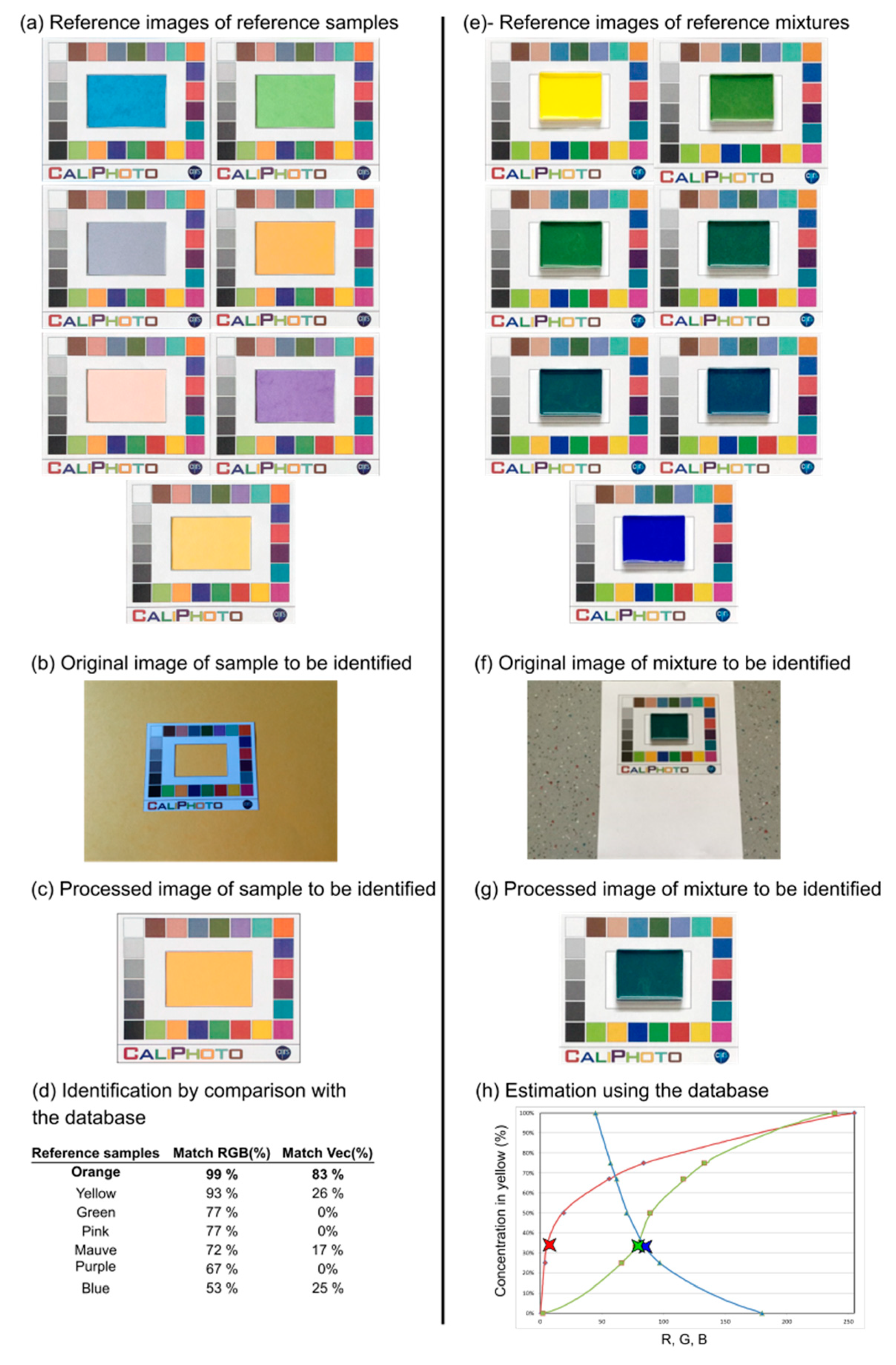
Appendix E. Material Identification Using the CaliPhoto Method
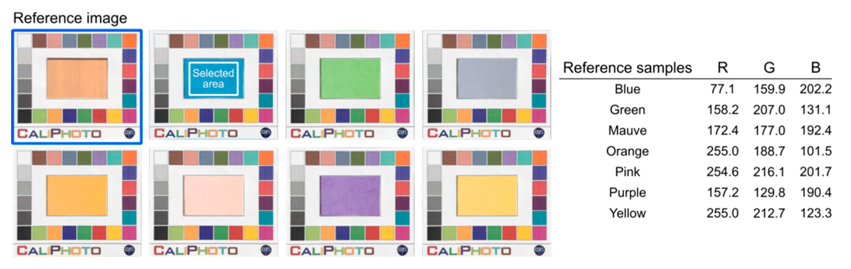
Appendix E.1. Identification using Average CaliPhoto Colour

| Sample | Blue | Green | Mauve | Orange | Pink | Purple | Yellow | Average Δ12 (%) |
|---|---|---|---|---|---|---|---|---|
| Dark skin | 0.51% | 0.39% | 0.69% | 0.69% | 0.74% | 0.23% | 1.49% | 0.68% |
| Light skin | 1.51% | 1.76% | 2.07% | 2.22% | 1.10% | 1.65% | 1.21% | 1.65% |
| Blue sky | 1.47% | 1.56% | 1.84% | 2.47% | 0.38% | 1.23% | 0.11% | 1.29% |
| Foliage | 1.50% | 1.62% | 1.50% | 1.64% | 0.39% | 1.30% | 1.08% | 1.29% |
| Blue flower | 0.37% | 0.28% | 0.21% | 0.72% | 0.55% | 0.18% | 0.60% | 0.42% |
| Bluish green | 0.83% | 1.84% | 1.79% | 3.71% | 1.94% | 1.19% | 2.58% | 1.98% |
| Orange | 2.02% | 1.37% | 1.19% | 1.92% | 1.39% | 1.49% | 1.94% | 1.62% |
| Purple red | 0.55% | 0.73% | 1.15% | 0.41% | 0.32% | 0.29% | 1.19% | 0.66% |
| Moderate red | 1.01% | 1.71% | 1.74% | 1.53% | 1.26% | 1.73% | 2.23% | 1.60% |
| Purple | 2.76% | 2.52% | 2.18% | 1.46% | 1.03% | 2.42% | 2.38% | 2.11% |
| Cyan | 0.64% | 0.80% | 0.71% | 2.42% | 1.52% | 0.65% | 1.57% | 1.19% |
| Magenta | 0.77% | 0.82% | 0.65% | 1.25% | 1.09% | 0.80% | 1.37% | 0.96% |
| Yellow | 0.63% | 0.61% | 0.55% | 0.14% | 0.42% | 0.79% | 0.25% | 0.48% |
| Red | 0.37% | 1.50% | 1.65% | 1.38% | 0.97% | 1.12% | 2.01% | 1.28% |
| Green | 0.79% | 0.76% | 0.67% | 0.88% | 1.49% | 0.69% | 1.21% | 0.93% |
| Blue | 1.06% | 1.30% | 1.95% | 0.89% | 1.11% | 0.98% | 0.75% | 1.15% |
| Orange yellow | 0.80% | 0.21% | 0.26% | 0.86% | 0.57% | 0.21% | 0.63% | 0.51% |
| Yellow green | 1.55% | 1.23% | 0.80% | 1.55% | 1.56% | 1.27% | 1.59% | 1.36% |
| Black | 0.97% | 0.73% | 0.56% | 0.45% | 0.42% | 0.81% | 0.62% | 0.65% |
| Dark grey | 1.54% | 0.81% | 0.88% | 1.54% | 0.33% | 0.87% | 0.41% | 0.91% |
| Grey | 1.99% | 2.31% | 2.47% | 3.45% | 1.19% | 2.00% | 1.84% | 2.18% |
| Light grey | 0.97% | 1.57% | 1.98% | 2.39% | 0.76% | 1.10% | 1.50% | 1.47% |
| Off-white | 0.80% | 1.04% | 1.26% | 1.27% | 0.36% | 0.94% | 0.58% | 0.89% |
| White | 0.18% | 0.28% | 0.38% | 0.31% | 0.11% | 0.36% | 0.16% | 0.25% |
| Δ (%) | 1.07% | 1.16% | 1.21% | 1.48% | 0.87% | 1.01% | 1.22% | 1.15% |
| Reference Samples | R | G | B | Uncertainties |
|---|---|---|---|---|
| blue | 77.1 | 159.9 | 202.2 | ±2.7 |
| green | 158.2 | 207.0 | 131.1 | ±3.0 |
| mauve | 172.3 | 177.0 | 192.4 | ±3.1 |
| orange | 255.0 | 188.7 | 101.5 | ±3.8 |
| pink | 254.6 | 216.1 | 201.6 | ±2.2 |
| purple | 157.2 | 129.8 | 190.4 | ±2.6 |
| yellow | 255.0 | 212.7 | 123.3 | ±3.1 |
| Sample to Identify | 255 | 191.69 | 101.81 | Orange | |
|---|---|---|---|---|---|
| Reference Samples | R | G | B | Δij (%) | Mij (%) |
| blue | 77.1 | 159.92 | 202.15 | 47% | 53% |
| green | 158.21 | 207.02 | 131.1 | 23% | 77% |
| mauve | 172.37 | 177.01 | 192.38 | 28% | 72% |
| orange | 255 | 188.66 | 101.49 | 1% | 99% |
| pink | 254.6 | 216.12 | 201.65 | 23% | 77% |
| purple | 157.21 | 129.81 | 190.44 | 33% | 67% |
| yellow | 255 | 212.7 | 123.3 | 7% | 93% |
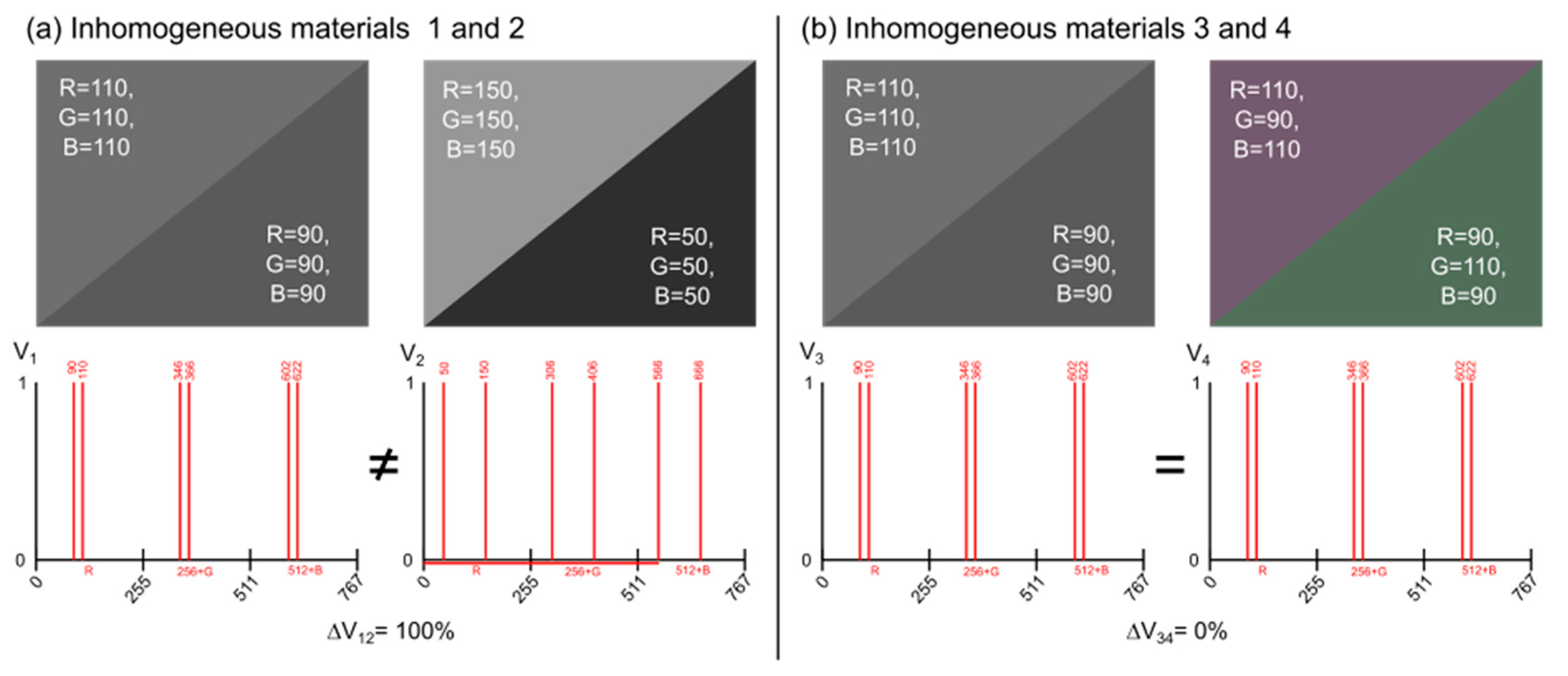
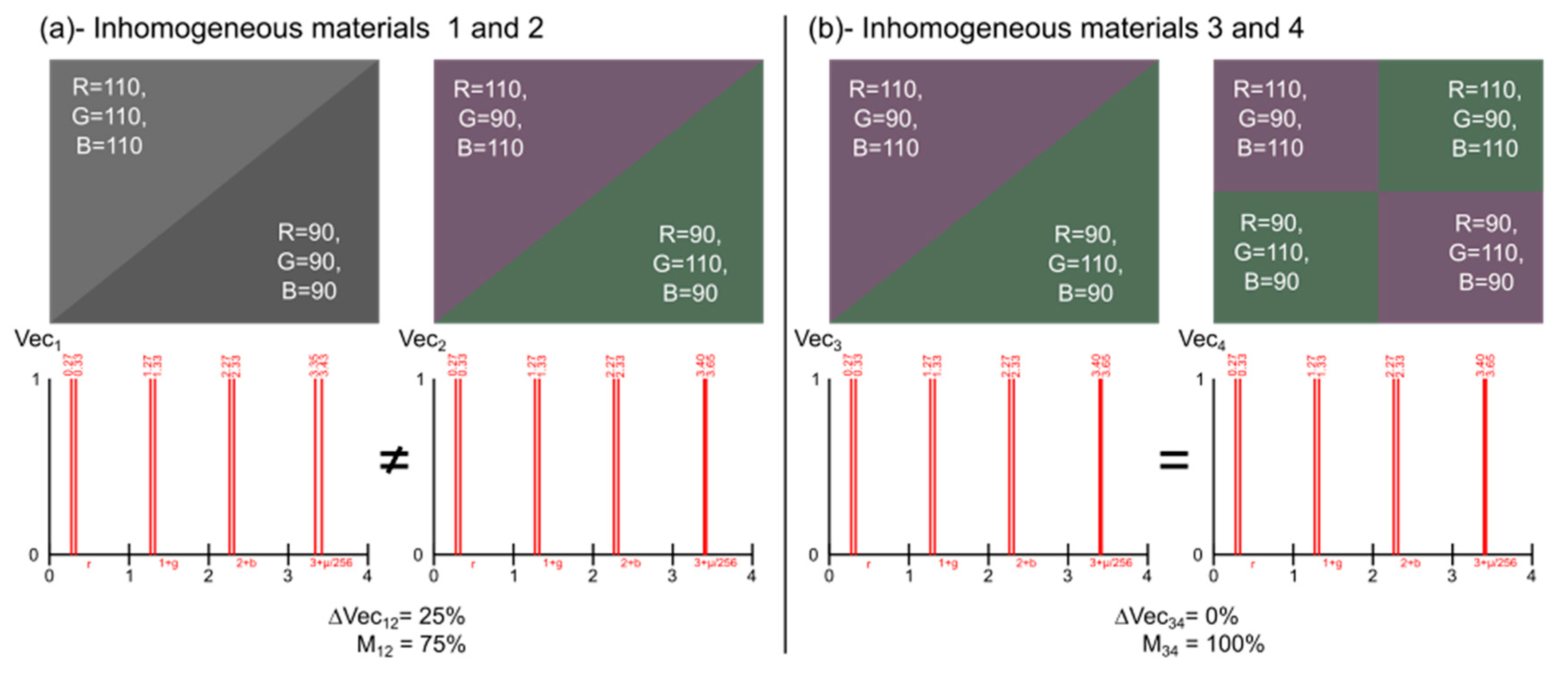
Appendix E.2. Identification Using CaliPhoto Colour Vectors


| Sample to Identify | Orange |
|---|---|
| Reference Samples | Mij (%) |
| blue | 25% |
| green | 0% |
| mauve | 17% |
| orange | 83% |
| pink | 0% |
| purple | 0% |
| yellow | 26% |
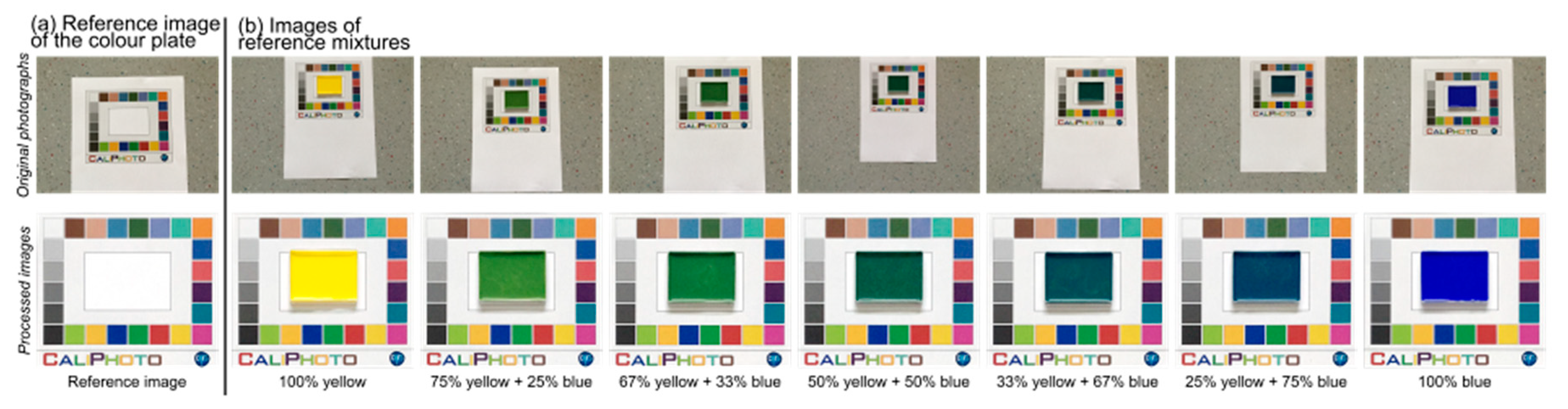
Appendix F. Precharacterisation of Materials Using the CaliPhoto Method

| Reference Mixtures | Concentration in Yellow | Concentration Uncertainties | RC | GC | BC | (RGB)C Uncertainties |
|---|---|---|---|---|---|---|
| 100% blue | 0% | 0% | 0.04 | 1.33 | 180.17 | 1.8 |
| 25% yellow–75% blue | 25% | 1% | 3.26 | 65,52 | 96.98 | 2.3 |
| 33% yellow–67% blue | 33% | 1% | 5.24 | 77.59 | 85.69 | 2.0 |
| 50% yellow–50% blue | 50% | 2% | 18,13 | 88.93 | 69.67 | 1.8 |
| 67% yellow–33% blue | 67% | 1% | 56.88 | 117.34 | 61.57 | 2.3 |
| 75% yellow–25% blue | 75% | 1% | 84.77 | 134.25 | 57.24 | 1.5 |
| 100% yellow | 100% | 0% | 255.00 | 239.87 | 45.09 | 1.8 |
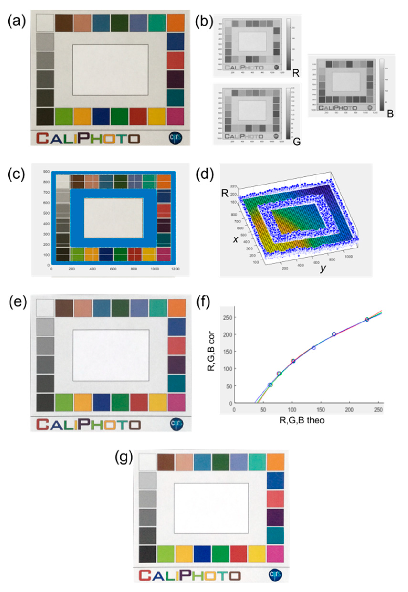
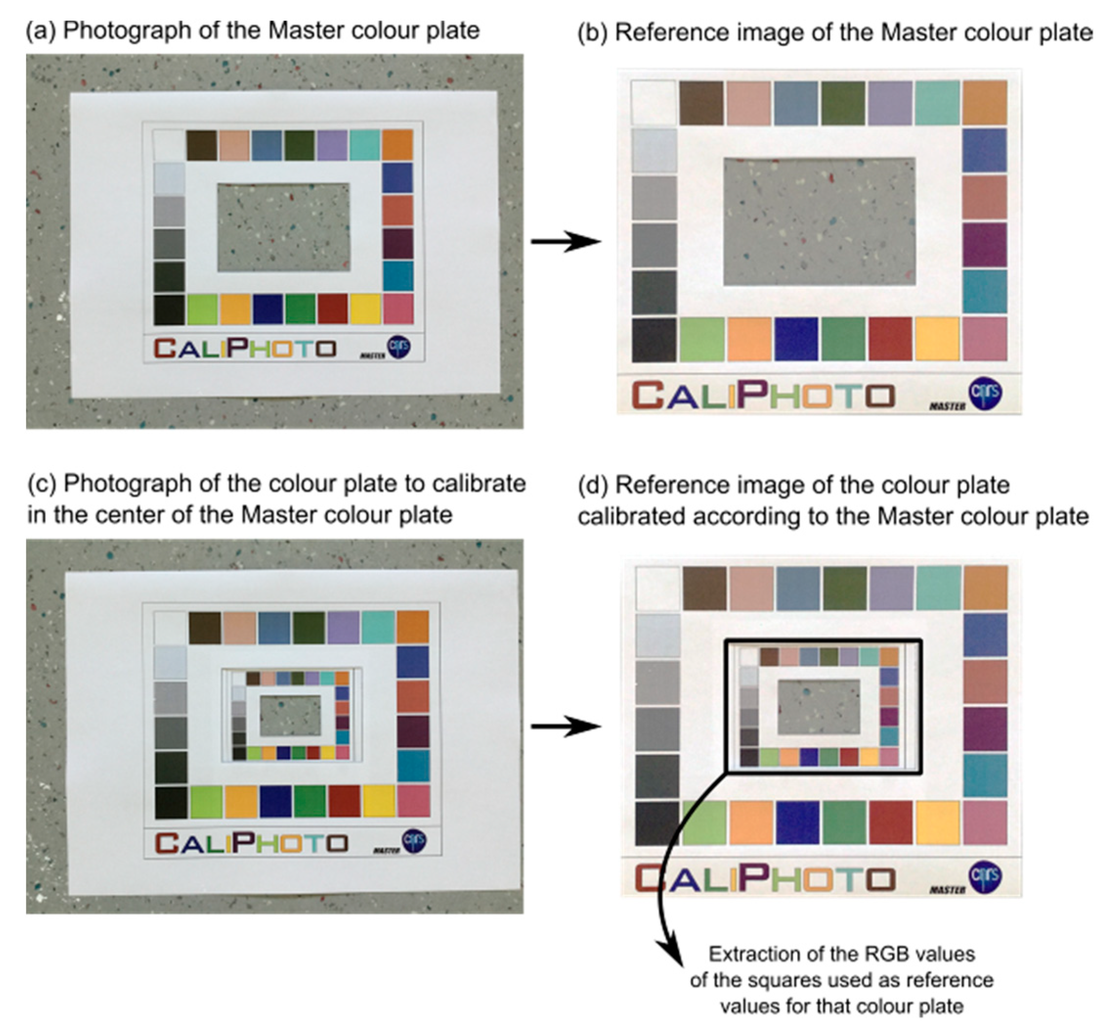
Appendix G. Creation of a Master Colour Plate for the CaliPhoto Method
- Print a colour plate sufficiently large to place the colour plates used for your application in the window. This large colour plate will now become your Master Colour plate and must be kept secure (Figure A15a).
- Apply the CaliPhoto process defined in Appendix B in order to obtain a reference image of the Master Colour plate (Figure A15b).
- Make a good-quality image of the new colour plate, which will be used for scientific investigations, placed in the centre of the Master Colour plate (Figure A15c).
- Calibrate the image of the new colour plate using the Master Colour plate and the CaliPhoto image processing defined in Appendix C (Figure A15d).
- Use the image of the colour plate in the centre of the Master Colour plate as a reference image.
- In case of a lost or irreversibly altered colour plate, print a new colour plate and redo steps 1 to 5.

References
- Leon, K.; Mery, D.; Pedreschi, F.; Leon, J. Color measurement in L*a*b* units from RGB digital images. Food Res. Int. 2006, 39, 1084–1091. [Google Scholar] [CrossRef]
- Gökay, M.K.; Gundogdu, I.B. Color identification of some Turkish marbles. Constr. Build. Mater. 2008, 22, 1342–1349. [Google Scholar] [CrossRef]
- Bianconi, F.; Gonzalez, F.; Fernandez, A.; Saetta, S.A. Automatic classification of granite tiles through colour and texture features. Expert Syst. Appl. 2012, 39, 11212–11218. [Google Scholar] [CrossRef]
- Furferi, R. Color Classification Method for recycled Melange Fabrics. J. Appl. Sci. 2011, 11, 236–246. [Google Scholar]
- Kempe, D.B. Colorimetric characterisation of flatbed scanners for rock/sediment imaging. Comput. Geosci. 2014, 67, 69–74. [Google Scholar] [CrossRef]
- Haeghen, Y.V.; Naeyaert, J.M.; Lemahieu, I.; Philips, W. An imaging system with calibrated color image acquisition for use in dermatology. IEEE Trans. Med. Imaging 2000, 19, 722–730. [Google Scholar] [CrossRef] [PubMed]
- Iñigo, A.C.; García-Talegón, J.; Vicente-Tavera, S.; Martín-González, S.; Casado-Marín, S.; Vargas-Muñoz, M.; Pérez-Rodríguez, J.L. Colour and ultrasound propagation speed changes by different ageing of freezing/thawing and cooling/heating in granitic materials. Cold Reg. Sci. Technol. 2013, 85, 71–78. [Google Scholar] [CrossRef]
- Oestmo, S. Digital imaging technology and experimental archeology: A methodological framework for the identification and interpretation of fire modified rock (FMR). J. Archaeol. Sci. 2013, 40, 4429–4443. [Google Scholar] [CrossRef]
- McCamy, C.S.; Marcus, H.; Davidson, J.G. A Color-Rendition Chart. J. Appl. Photogr. Eng. 1976, 2, 95–99. [Google Scholar]
- X-Rite. ColorChecker Camera Calibration. Available online: https://xritephoto.com/colorchecker-classic (accessed on 7 November 2019).
- Morris, V.J.; Kirby, A.R.; Gunning, A.P. Basic Principles. In Atomic Force Microscopy for Biologists; Imperial College Press: London, UK, 1999; pp. 70–71. [Google Scholar]
- Wannous, H.; Treuillet, S.; Lucas, Y.; Mansouri, A.; Voisin, Y. Design of a Customized Pattern for Improving Color Constancy Across Camera and Illumination Changes. In Proceedings of the VISAPP 2010—Fifth International Conference on Computer Vision Theory and Applications, Angers, France, 25 May 2010. [Google Scholar]
- Josset, J.-L.; Westall, F.; Hofmann, B.A.; Spray, J.; Cockell, C.; Kempe, S.; Griffiths, A.D.; De Sanctis, M.C.; Colangeli, L.; Koschny, D.; et al. The Close-Up Imager Onboard the ESA ExoMars Rover: Objectives, Description, Operations, and Science Validation Activities. Astrobiology 2017, 17, 595–611. [Google Scholar] [CrossRef] [PubMed]


© 2019 by the authors. Licensee MDPI, Basel, Switzerland. This article is an open access article distributed under the terms and conditions of the Creative Commons Attribution (CC BY) license (http://creativecommons.org/licenses/by/4.0/).
Share and Cite
Foucher, F.; Guimbretière, G.; Bost, N.; Hickman-Lewis, K.; Courtois, A.; Luengo, L.; Marceau, E.; Bergounioux, M.; Westall, F. The CaliPhoto Method. Inventions 2019, 4, 67. https://doi.org/10.3390/inventions4040067
Foucher F, Guimbretière G, Bost N, Hickman-Lewis K, Courtois A, Luengo L, Marceau E, Bergounioux M, Westall F. The CaliPhoto Method. Inventions. 2019; 4(4):67. https://doi.org/10.3390/inventions4040067
Chicago/Turabian StyleFoucher, Frédéric, Guillaume Guimbretière, Nicolas Bost, Keyron Hickman-Lewis, Aurélie Courtois, Lydie Luengo, Etienne Marceau, Maïtine Bergounioux, and Frances Westall. 2019. "The CaliPhoto Method" Inventions 4, no. 4: 67. https://doi.org/10.3390/inventions4040067
APA StyleFoucher, F., Guimbretière, G., Bost, N., Hickman-Lewis, K., Courtois, A., Luengo, L., Marceau, E., Bergounioux, M., & Westall, F. (2019). The CaliPhoto Method. Inventions, 4(4), 67. https://doi.org/10.3390/inventions4040067