A Thermodynamic Model for Lithium-Ion Battery Degradation: Application of the Degradation-Entropy Generation Theorem


Abstract
1. Introduction
Background/Literature Review
2. Degradation-Entropy Generation Theorem Review
2.1. Statement
2.2. Generalized Degradation Analysis Procedure
- It identifies the degradation measure w, dissipative process energies and phenomenological variables ;
- It finds the entropy generation = () caused by the dissipative processes ;
- It evaluates the coefficients by measuring increments, accumulation or rates of degradation versus increments, accumulation or rates of entropy generation;
- It relates degradation measure to entropy generation, via Equations (7) or (9).
3. Formulations
3.1. Fundamental Thermodynamic Formulations
3.1.1. First Law—Energy Conservation
3.1.2. Second Law and Entropy Balance—Irreversible Entropy Generation
3.1.3. Combining First and Second Laws
3.2. Li-Ion Battery Analysis
3.2.1. Combining First and Second Laws with Gibbs Potential
3.2.2. Relaxation/Settling and Self Discharge
3.3. Entropy Content S and Internal Free Energy Dissipation −SdT
3.4. Degradation-Entropy Generation (DEG) and Capacity Fade in Batteries
- Let available battery capacity or charge content be a DEG transformation measure and capacity fade (lost discharge/charge capacity) be the observed/measured degradation, the DEG Equation (9), with replacing w becomes,
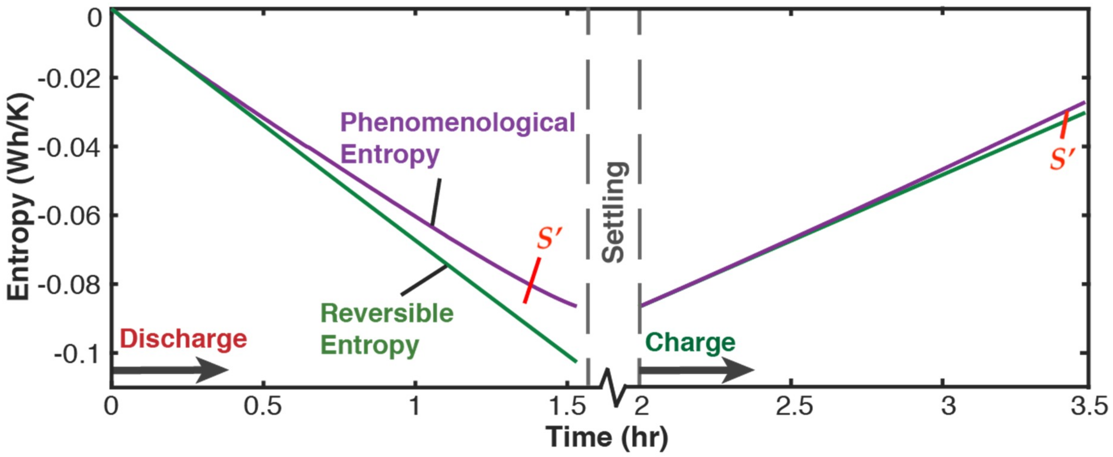
- From Equation (41), entropy generation S’ = S’, suggesting via Equation (43) that = . Substituting the entropy generation terms of Equation (41) into Equation (43) gives
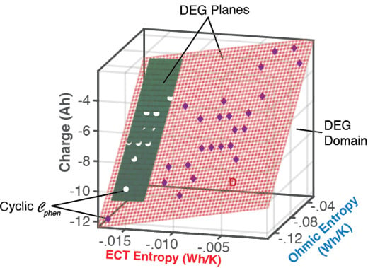
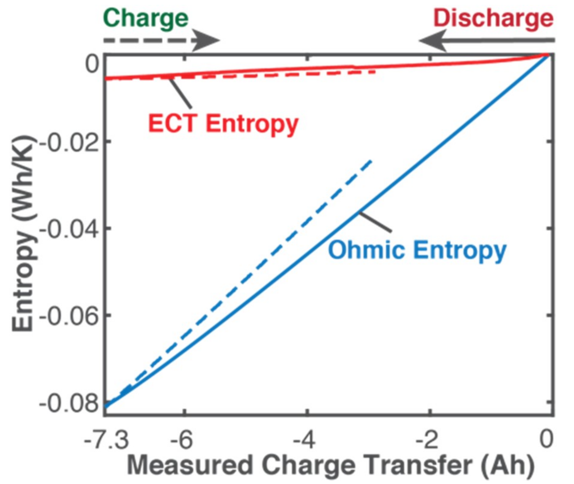
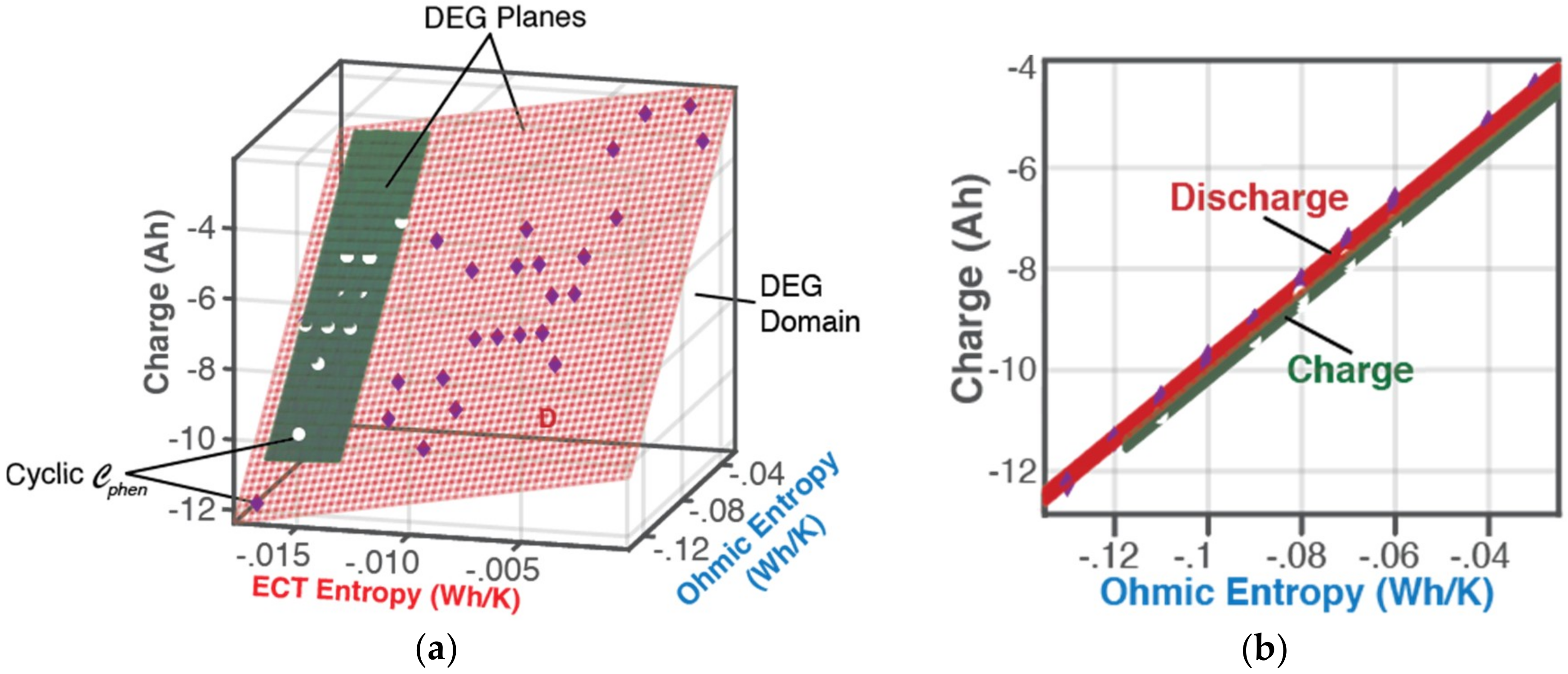
- Via Equation (8), with replacing w, DEG coefficientscan be evaluated via measurements, as slopes of charge versus ECT entropy , Ohmic entropy and reversible Gibbs entropy . As demonstrated in Section 4, the DEG capacity fade, Equation (44), is applicable to all forms of cycling conditions.
4. Experiments
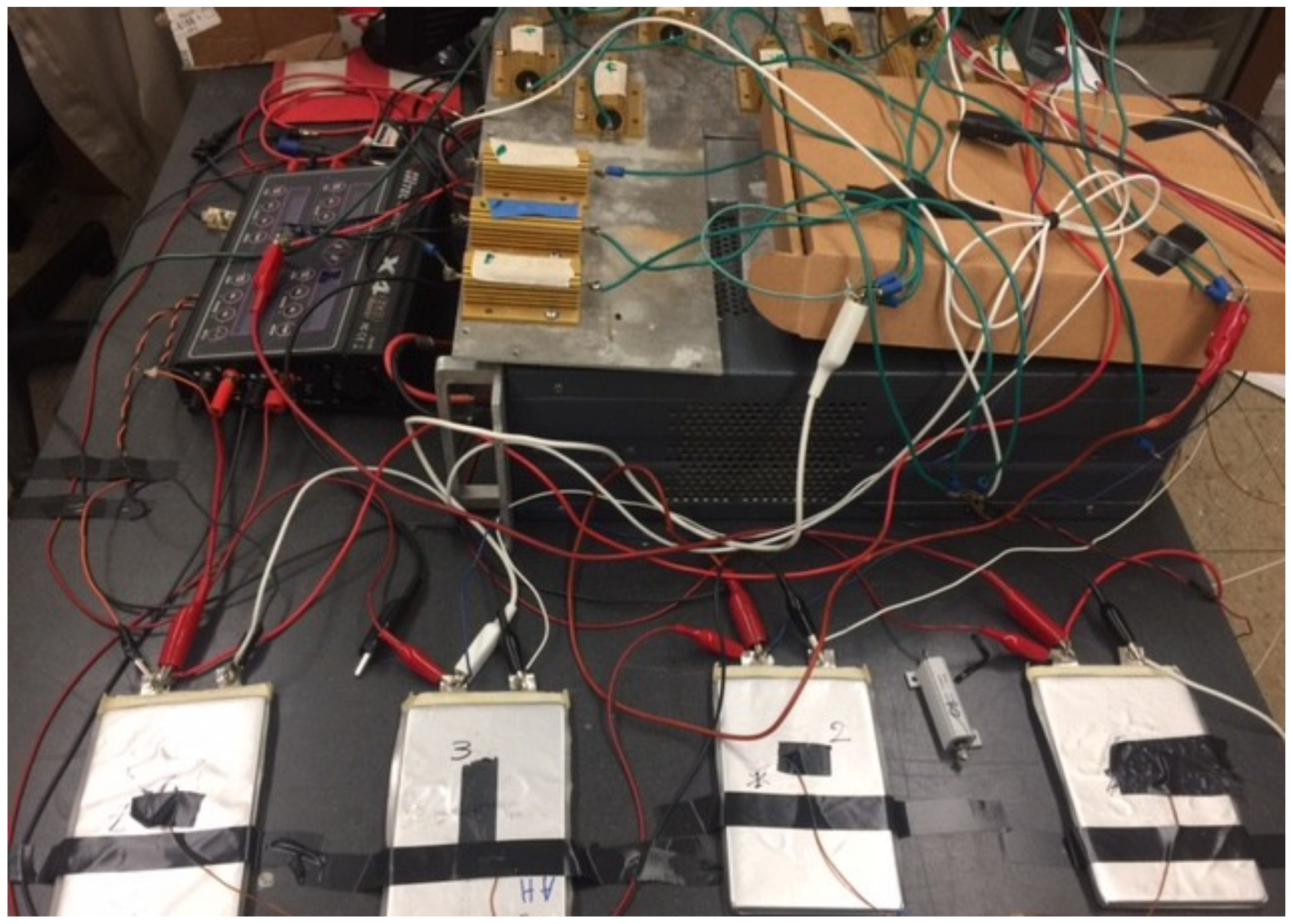
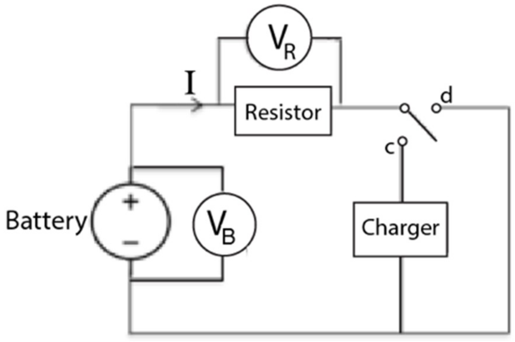
4.1. Apparatus
4.2. Setup and Procedure
4.2.1. Setup and Initial Measurements
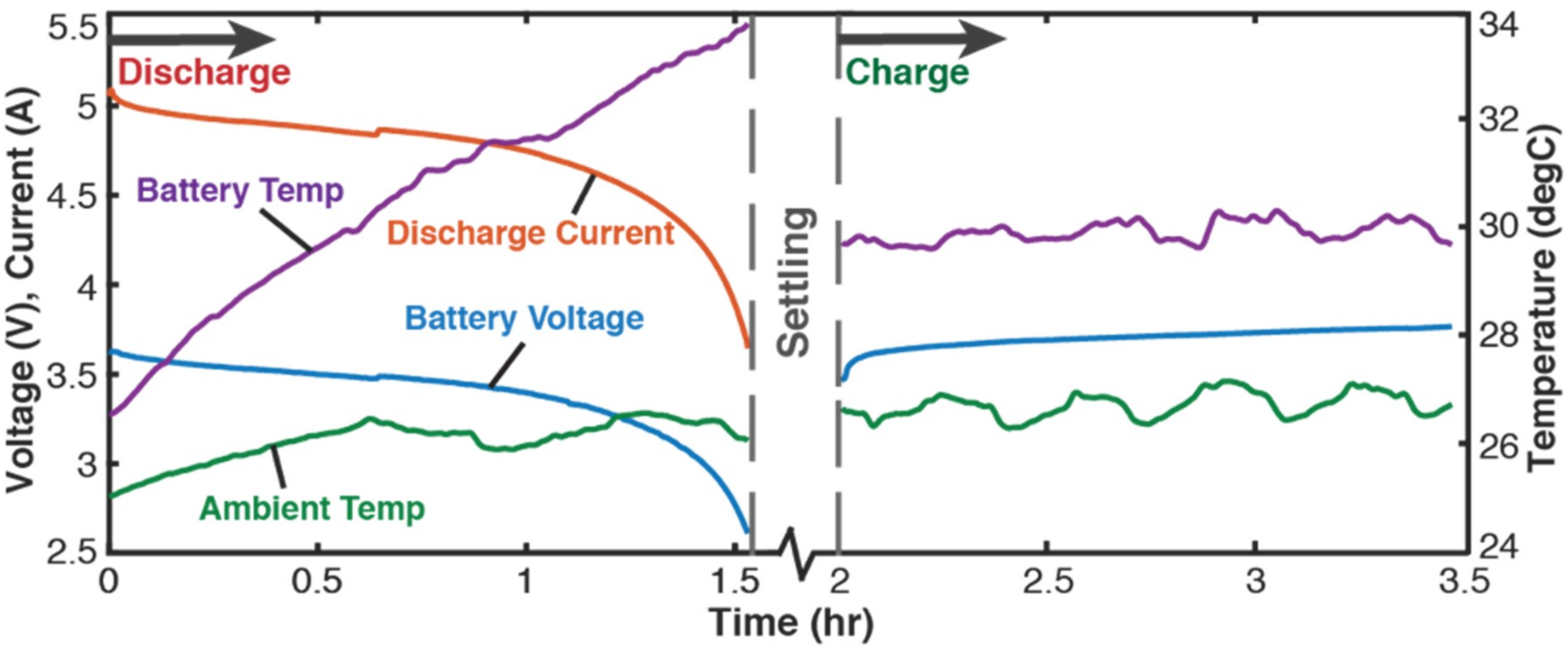
4.2.2. Cycling
- the battery’s capacity fell to less than two-thirds the initial capacity or
- the battery began to inflate in geometric volume (close monitoring of Li-ion batteries was required during cycling).
5. Results, Analysis, and Discussion
5.1. Gibbs Energy and Entropy Components
5.2. DEG—Capacity Versus Entropy
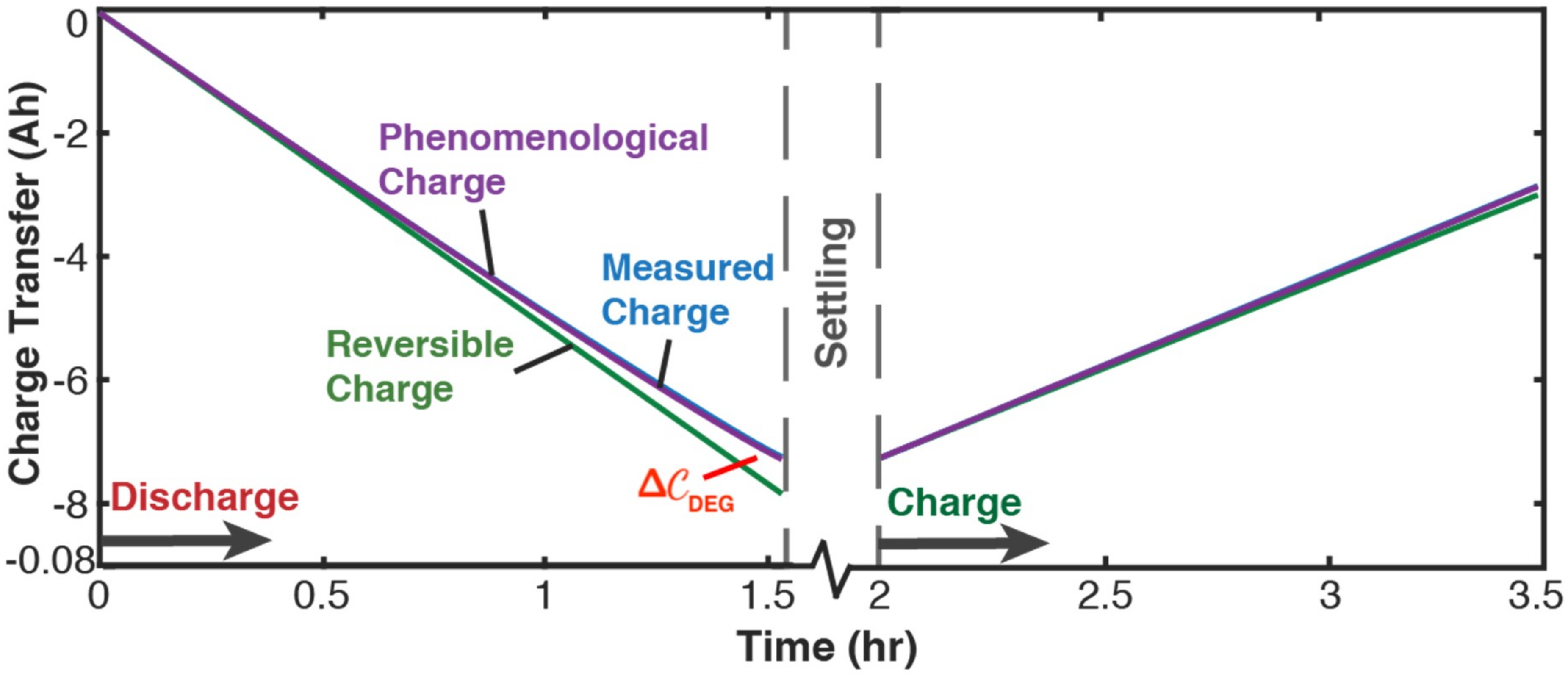
5.2.1. Phenomenological Charge, Measured Charge, and Reversible Charge
5.2.2. Evaluating Capacity Fade—Battery Cycle Life Model
- Cyclic values of DEG capacity fade and Coulomb-Counted capacity fade presented in Table 2 for cycles 1 to 32, were obtained as follows:
- Evaluate phenomenological charge in Table 2, columns 2 (discharge) and 7 (charge), from Equation (47), by combining reference DEG coefficients with each cycle’s phenomenological entropy components and given in Table 1. For example, the discharge step of cycle 6, row 6 of Table 1, has −0.08 Wh/K, and –0.005 Wh/K. When combined with Ah K/Wh and Ah K/Wh from cycle 1, Equation (47) gives = (76.6 × −0.08) + (113 × −0.005) = −6.7 Ah.
- Evaluate reversible charge (Table 2, columns 3 and 8) from Equation (49). For example, the cycle 1 starting current = −5.2 A gives the cycle 6 discharge −5.2 A which, with the cycle 6 discharge duration = 1.53 h (Table A1 in Appendix B), gives = −5.2 × 1.53= −8.0 Ah.
- Evaluate DEG capacity fade (Table 2, columns 4 and 9) from Equation (51), . For cycle 6 discharge, −6.7 − (−8.0) = 1.3 Ah. Similarly, for cycle 6 charge, 0.3 Ah.
- Evaluate Coulomb-Counted capacity fade (Table 2, column 6) from Equation (42), , where −6.1 Ah is Coulomb-Counted charge transfer during cycle 1 discharge. For cycle 6, = |−6.1| − |−7.2| = −1.1 Ah.
6. Discussion
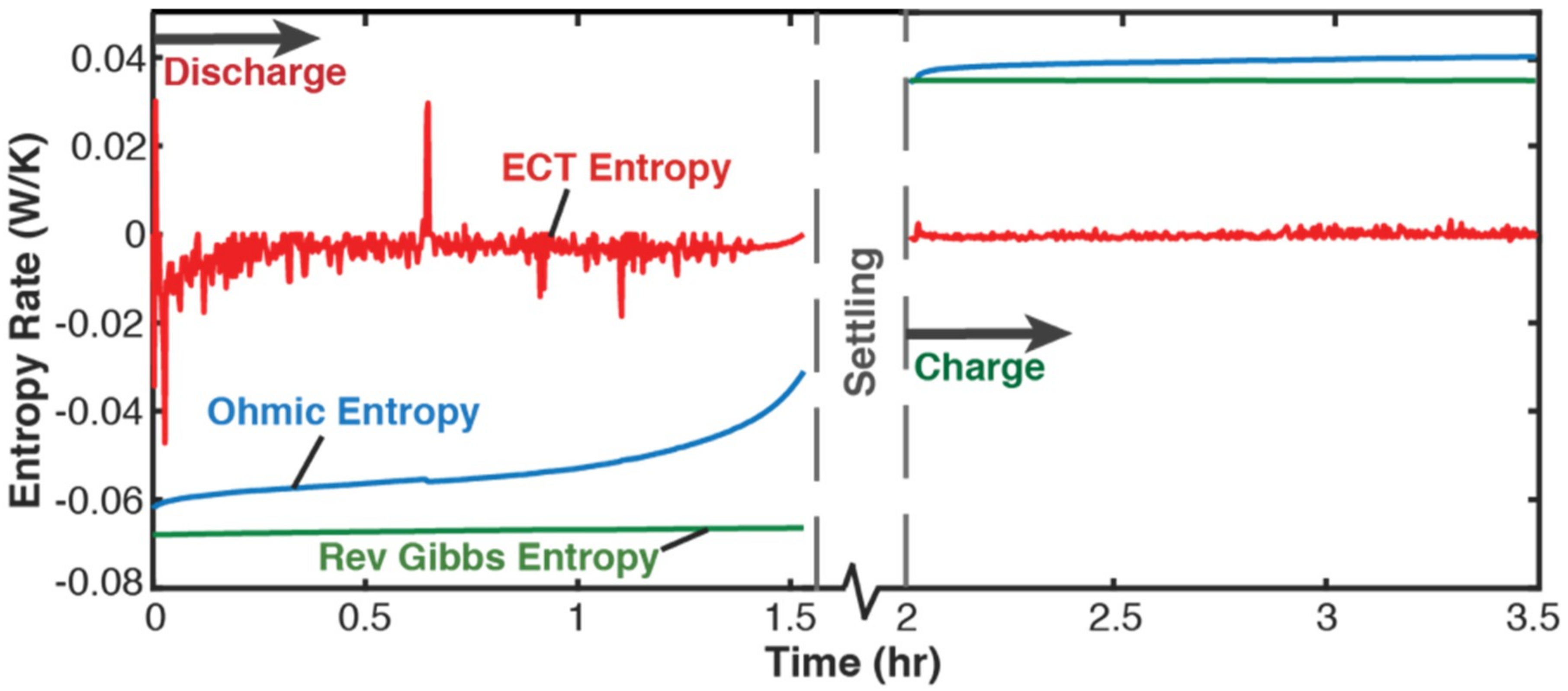
- phenomenological entropy generation is the sum of Ohmic entropy and electro-chemico-thermal ECT entropy S′VT;
- entropy generation is the difference between phenomenological and reversible Gibbs entropies, at every instant;
- entropy generation is always non-negative, in accordance with the second law, whereas components and are directional—positive during charge and negative during discharge. This implies during charge and during discharge, in accordance with experience and thermodynamic laws. This article demonstrated the significance of the previously neglected reversible and ECT entropies in evaluating entropy generation in batteries.
6.1. Features of the DEG Theorem and Coefficients
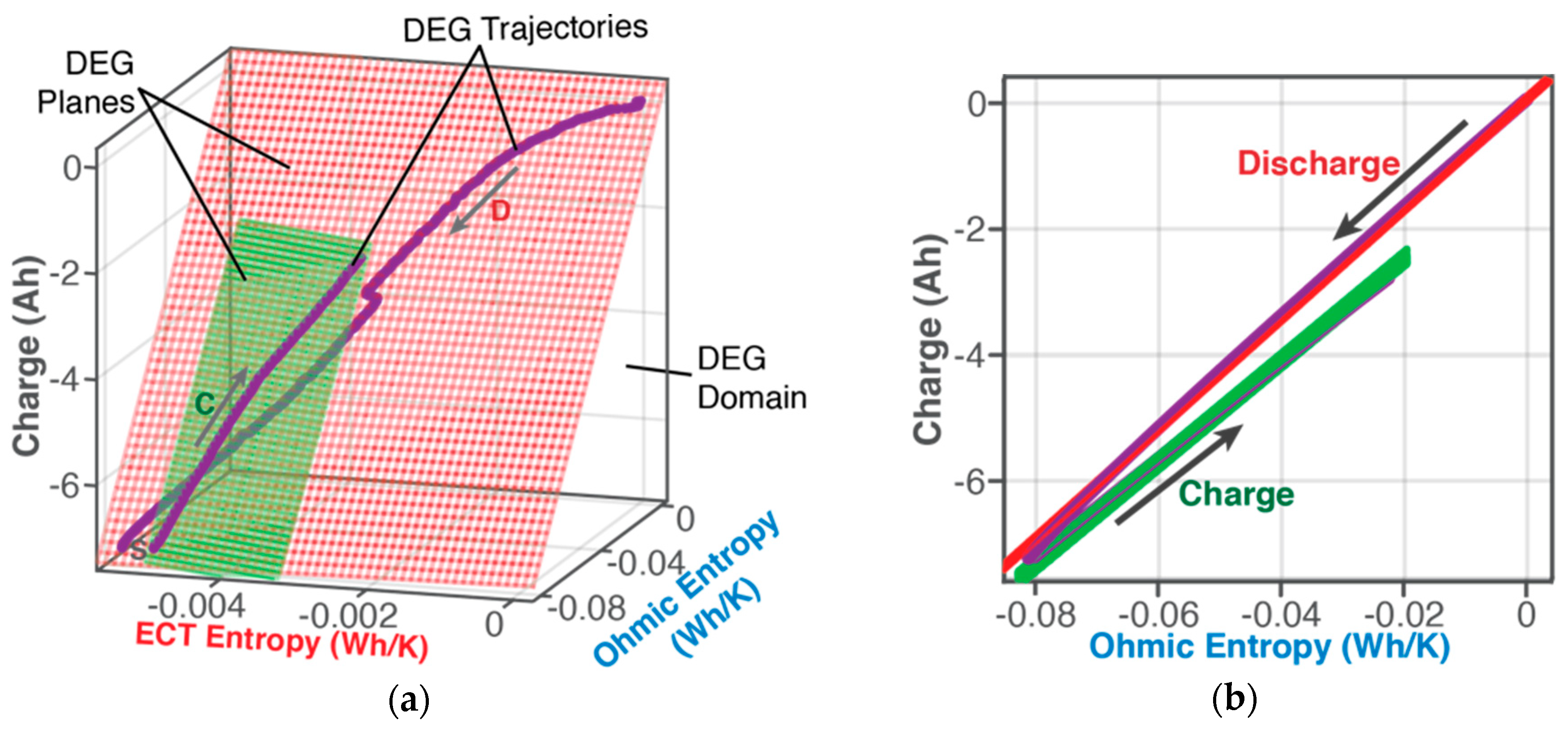
6.1.1. DEG Trajectories, Surfaces, and Domains
7. Summary and Conclusions
Author Contributions
Acknowledgments
Conflicts of Interest
Abbreviations
| Nomenclature | Name | Unit |
| chemical affinity | J/mol | |
| B | DEG coefficient | Ah K/Wh |
| charge, charge transfer or capacity | Ah | |
| charge or capacity fade | Ah | |
| F | Faraday’s constant | C/mol |
| G | Gibbs energy | Wh |
| I | discharge/charge current or rate | A |
| kB | Boltzmann constant | J/K |
| m | mass | kg |
| n’ | number of charge species | |
| N | cycle number | Kg/mol |
| N, Nk | number of moles of substance | mol |
| p | dissipative process energy | J |
| P | pressure | Pa |
| q | charge | Ah |
| Q | heat | J |
| R | gas constant | J/mol·K |
| S | entropy or entropy content | Wh/K |
| S’ | entropy generation or production | Wh/K |
| t | time | sec |
| T | temperature | degC or K |
| U | internal energy | J |
| V | voltage | V |
| volume | m3 | |
| w | degradation measure | |
| W | work | J |
| Symbols | ||
| μ | chemical potential | |
| ζ | phenomenological variable | |
| Subscripts & acronyms | ||
| Ω | Ohmic | |
| 0 | initial | |
| c | charge | |
| d | discharge | |
| ECT, VT | Electro-Chemico-Thermal | |
| t | time | |
| rev | reversible | |
| irr | irreversible | |
| phen | phenomenological | |
| CC | Coulomb-Counted | |
| DEG | Degradation-Entropy Generation |
Appendix A
Appendix A.1. Electrochemical Kinetics
Appendix A.1.1. Charge Intercalation (Absorption) and Deintercalation (Release)
Appendix A.1.2. Reaction Rates
Appendix A.1.3. Charge Transport
Appendix A.2. Coupling Reaction and Transport Kinetics with the Electrochemical Potential
Appendix B
Experimental Results

| Discharge | Charge | ||||||||||||
|---|---|---|---|---|---|---|---|---|---|---|---|---|---|
| N | h | Ah | Wh | degC | degC | V | SoH | hr | Ah | Wh | degC | degC | |
| 1 | 1.47 | −6.10 | −19.9 | 6.5 | 25.9 | 0.77 | 0.042 | 1.00 | 3.49 | 10.47 | 41.4 | 0.2 | 27.6 |
| 2 | 1.79 | −8.37 | −28.6 | 10.2 | 24.8 | 2.43 | 0.025 | 0.98 | 1.72 | 5.14 | 20.2 | 0.8 | 26.7 |
| 3 | Half cycle | 1.33 | 3.97 | 16.1 | 8.1 | 25.7 | |||||||
| 4 | 2.00 | −9.52 | −32.9 | 6.2 | 27.8 | 2.66 | 0.031 | 0.98 | 1.28 | 3.83 | 15.1 | −2.7 | 27.7 |
| 5 | 0.64 | −3.00 | −10.2 | 8.6 | 24.6 | 2.69 | 0.081 | 0.95 | 1.81 | 5.42 | 21.8 | −0.3 | 26.5 |
| 6 | 1.53 | −7.23 | −24.6 | 7.2 | 26.1 | 2.61 | 0.026 | 0.97 | 1.47 | 4.41 | 17.4 | 0.4 | 26.7 |
| 7 | 1.40 | −6.71 | −22.9 | 6.8 | 24.8 | 2.67 | 0.032 | 0.99 | 2.73 | 8.17 | 32.8 | 0.0 | 25.3 |
| 8 | 2.03 | −9.74 | −33.4 | 8.8 | 24.6 | 2.64 | 0.028 | 1.00 | Missing data | ||||
| 9 | 1.36 | −6.39 | −21.5 | 6.3 | 24.9 | 2.58 | 0.026 | 0.98 | 3.60 | 10.80 | 43.3 | 2.6 | 27.1 |
| 10 | 1.77 | −8.70 | −30.3 | 7.1 | 26.8 | 2.87 | 0.024 | 0.99 | 0.61 | 1.81 | 7.0 | −1.7 | 27.7 |
| 11 | 1.09 | −5.18 | −17.5 | 9.2 | 23.5 | 2.42 | 0.027 | 0.99 | 1.62 | 4.86 | 19.2 | 0.9 | 26.2 |
| 12 | 1.82 | −8.52 | −29.0 | 6.9 | 26.6 | 1.88 | 0.032 | 0.99 | 1.80 | 5.40 | 21.5 | 2.8 | 26.3 |
| 13 | Half cycle | 2.13 | 6.37 | 25.3 | −0.7 | 28.5 | |||||||
| 14 | 2.12 | −10.54 | −37.0 | 6.3 | 29.7 | 2.32 | 0.028 | 1.03 | 0.99 | 2.96 | 11.5 | −0.7 | 29.5 |
| 15 | 1.33 | −6.24 | −21.0 | 8.8 | 24.7 | 2.42 | 0.040 | 0.98 | 1.53 | 4.58 | 18.1 | −0.1 | 26.7 |
| 16 | 1.73 | −8.27 | −28.1 | 7.9 | 24.8 | 2.14 | 0.025 | 1.00 | 1.46 | 4.38 | 17.3 | −0.7 | 25.8 |
| 17 | 1.67 | −7.97 | −27.0 | 8.9 | 25.4 | 2.31 | 0.029 | 1.00 | 1.81 | 5.42 | 21.5 | −0.5 | 27.5 |
| 18 | 2.13 | −10.01 | −33.6 | 7.3 | 26.2 | 1.46 | 0.027 | 1.02 | 1.28 | 3.84 | 15.0 | 0.7 | 27.5 |
| 19 | 1.36 | −6.42 | −21.4 | 5.6 | 25.6 | 2.18 | 0.026 | 0.99 | 1.47 | 4.40 | 17.4 | −0.6 | 26.1 |
| 20 | 2.00 | −8.95 | −29.2 | 8.0 | 25.8 | 0.95 | 0.027 | 1.01 | 1.69 | 5.06 | 20.1 | 0.1 | 28.2 |
| 21 | 2.16 | −9.45 | −30.4 | 9.0 | 27.2 | 1.10 | 0.028 | 1.02 | 1.27 | 3.79 | 14.9 | −0.1 | 26.7 |
| 22 | 1.50 | −6.78 | −21.8 | 7.4 | 25.6 | 1.58 | 0.031 | 0.98 | 1.41 | 4.22 | 16.7 | 0.9 | 25.8 |
| 23 | 1.74 | −7.85 | −25.8 | 5.9 | 25.3 | 1.93 | 0.021 | 0.95 | 1.50 | 4.50 | 17.8 | 2.0 | 26.0 |
| 24 | 1.80 | −8.19 | −26.7 | 11.1 | 24.0 | 1.68 | 0.025 | 0.97 | 1.73 | 5.17 | 20.5 | −0.2 | 26.5 |
| 25 | 0.68 | −3.35 | −11.7 | 3.4 | 25.6 | 3.44 | 0.025 | 0.97 | 4.16 | 12.47 | 50.9 | 2.1 | 26.3 |
| 26 | 2.69 | −12.37 | −40.6 | 8.0 | 25.0 | 1.56 | 0.036 | 1.00 | 1.48 | 4.43 | 17.5 | 2.4 | 26.8 |
| 27 | 2.44 | −8.84 | −25.7 | 6.9 | 24.9 | 0.57 | 0.034 | 0.95 | 2.76 | 8.27 | 33.1 | 3.1 | 26.7 |
| 28 | Half cycle | 1.77 | 5.30 | 21.1 | 3.1 | 26.3 | |||||||
| 29 | 1.91 | −6.41 | −18.1 | 8.4 | 25.5 | 0.58 | 0.045 | 0.93 | 3.08 | 9.22 | 37.2 | 2.3 | 25.9 |
| 30 | 0.91 | −3.75 | −11.4 | 13.0 | 25.2 | 1.15 | 0.074 | 0.96 | 3.33 | 9.97 | 40.4 | 2.7 | 26.3 |
| 31 | 1.31 | −5.76 | −17.7 | 8.3 | 25.8 | 1.80 | 0.051 | 0.95 | 3.21 | 9.63 | 39.2 | 7.2 | 26.1 |
| 32 | 0.75 | −3.19 | −9.7 | 12.3 | 25.4 | 1.51 | 0.129 | 0.94 | 1.69 | 5.05 | 20.0 | 0.9 | 25.7 |
References
- Rahn, C.D.; Wang, C.Y. Battery Systems Engineering, 1st ed.; John Wiley & Sons Ltd.: Hoboken, NJ, USA, 2013. [Google Scholar] [CrossRef]
- Huggins, R.A. Energy Storage: Fundamentals, Materials and Applications, 2nd ed.; Springer: New York, NY, USA, 2010. [Google Scholar] [CrossRef]
- Ménard, L.; Fontès, G.; Astier, S. Dynamic energy model of a lithium-ion battery. Math. Comput. Simul. 2010, 81, 327–339. [Google Scholar] [CrossRef]
- Bresser, D.; Paillard, E.; Passerini, S. Lithium-ion batteries (LIBs) for medium- and large-scale energy storage: Current cell materials and components. In Advances in Batteries for Medium and Large-Scale Energy Storage; Elsevier Ltd.: Amsterdam, The Netherlands, 2014; Volume 1, pp. 125–211. [Google Scholar] [CrossRef]
- Goodenough, J.B. Energy storage materials: A perspective. Energy Storage Mater. 2015, 1, 158–161. [Google Scholar] [CrossRef]
- Bresser, D.; Paillard, E.; Passerini, S. Lithium-ion batteries (LIBs) for medium- and large-scale energy storage: Emerging cell materials and components. In Advances in Batteries for Medium and Large-Scale Energy Storage; Menictas, C., Skyllas-Kazacos, M., Lim, T.M., Eds.; Elsevier Ltd.: Amsterdam, The Netherlands, 2014; Volume 1, pp. 213–289. [Google Scholar] [CrossRef]
- Kurzweil, P. Lithium battery energy storage: State of the art including lithium-air and lithium-sulfur systems. In Electrochemical Energy Storage for Renewable Sources and Grid Balancing, 1st ed.; Moseley, P.T., Garche, G., Eds.; Elsevier B.V.: Amsterdam, The Netherlands, 2014; pp. 269–307. [Google Scholar] [CrossRef]
- Goodenough, J.B.; Kim, Y. Challenges for rechargeable batteries. J. Power Sources 2011, 196, 6688–6694. [Google Scholar] [CrossRef]
- Scrosati, B.; Garche, J. Lithium batteries: Status, prospects and future. J. Power Sources 2010, 195, 2419–2430. [Google Scholar] [CrossRef]
- Vetter, J.; Novák, P.; Wagner, M.R.; Veit, C.; Möller, K.C.; Besenhard, J.O.; Winter, M.; Wohlfahrt-Mehrens, M.; Vogler, C.; Hammouche, A. Ageing mechanisms in lithium-ion batteries. J. Power Sources 2005, 147, 269–281. [Google Scholar] [CrossRef]
- Jiang, J.; Zhang, C. Fundamentals and Applications of Lithium-Ion Batteries in Electric Drive Vehicles; John Wiley & Sons Singapore Pte Ltd.: Singapore, 2015. [Google Scholar] [CrossRef]
- Barsukov, Y. Challenges and Solutions in Battery Fuel Gauging; 2004. Available online: http://www.ti.com/lit/ml/slyp086/slyp086.pdf (accessed on 29 March 2019).
- Miranda, D.; Costa, C.M.; Lanceros-Mendez, S. Lithium ion rechargeable batteries: State of the art and future needs of microscopic theoretical models and simulations. J. Electroanal. Chem. 2015, 739, 97–110. [Google Scholar] [CrossRef]
- Ecker, M.; Gerschler, J.B.; Vogel, J.; Käbitz, S.; Hust, F.; Dechent, P.; Sauer, D.U. Development of a lifetime prediction model for lithium-ion batteries based on extended accelerated aging test data. J. Power Sources 2012, 215, 248–257. [Google Scholar] [CrossRef]
- Cordoba-Arenas, A.; Onori, S.; Guezennec, Y.; Rizzoni, G. Capacity and power fade cycle-life model for plug-in hybrid electric vehicle lithium-ion battery cells containing blended spinel and layered-oxide positive electrodes. J. Power Sources 2015, 278, 473–483. [Google Scholar] [CrossRef]
- Panchal, S.; McGrory, J.; Kong, J.; Dincer, I.; Agelin-Chaab, M.; Fraser, R.; Fowler, M. Cycling degradation testing and analysis of a LiFePO4 battery at actual conditions. Int. J. Energy Res. 2017, 41, 2565–2575. [Google Scholar] [CrossRef]
- Panchal, S.; Rashid, M.; Long, F.; Mathew, M.; Fraser, R.; Fowler, M. Degradation Testing and Modeling of 200 Ah LiFePO4 Battery; SAE Technical Paper; SAE International: Detroit, MI, USA, 2018. [Google Scholar] [CrossRef]
- Karnopp, D. Bond graph models for electrochemical energy storage: Electrical, chemical and thermal effects. J. Frankl. Inst. 1990, 327, 983–992. [Google Scholar] [CrossRef]
- Kondepudi, D.; Prigogine, I. Modern Thermodynamics: From Heat Engines to Dissipative Structures; John Wiley & Sons Ltd.: Hoboken, NJ, USA, 1998. [Google Scholar]
- Esperilla, J.J.; Félez, J.; Romero, G.; Carretero, A. A full model for simulation of electrochemical cells including complex behavior. J. Power Sources 2007, 165, 436–445. [Google Scholar] [CrossRef]
- Ramadass, P.; Haran, B.; White, R.; Popov, B.N. Capacity fade of Sony 18650 cells cycled at elevated temperatures: Part II. Capacity fade analysis. J. Power Sources 2002, 112, 614–620. [Google Scholar] [CrossRef]
- Feng, X.; Gooi, H.B.; Chen, S. Capacity fade-based energy management for lithium-ion batteries used in PV systems. Electr. Power Syst. Res. 2015, 129, 150–159. [Google Scholar] [CrossRef]
- Ashwin, T.R.; Chung, Y.M.; Wang, J. Capacity fade modelling of lithium-ion battery under cyclic loading conditions. J. Power Sources 2016, 328, 586–598. [Google Scholar] [CrossRef]
- Long, L.; Wang, S.; Xiao, M.; Meng, Y. Polymer electrolytes for lithium polymer batteries. J. Mater. Chem. A 2016, 4, 10038–10069. [Google Scholar] [CrossRef]
- Schmalstieg, J.; Käbitz, S.; Ecker, M.; Sauer, D.U. A holistic aging model for Li(NiMnCo)O2 based 18650 lithium-ion batteries. J. Power Sources 2014, 257, 325–334. [Google Scholar] [CrossRef]
- Ecker, M.; Nieto, N.; Käbitz, S.; Schmalstieg, J.; Blanke, H.; Warnecke, A.; Sauer, D.U. Calendar and cycle life study of Li(NiMnCo)O2-based 18650 lithium-ion batteries. J. Power Sources 2014, 248, 839–851. [Google Scholar] [CrossRef]
- Käbitz, S.; Gerschler, J.B.; Ecker, M.; Yurdagel, Y.; Emmermacher, B.; André, D.; Mitsch, T.; Sauer, D.U. Cycle and calendar life study of a graphite|LiNi1/3Mn 1/3Co1/3O2 Li-ion high energy system. Part A: Full cell characterization. J. Power Sources 2013, 239, 572–583. [Google Scholar] [CrossRef]
- Bryant, M.D.; Khonsari, M.M.; Ling, F.F. On the thermodynamics of degradation. Proc. R. Soc. A: Math. Phys. Eng. Sci. 2008, 464, 2001–2014. [Google Scholar] [CrossRef]
- Strutt, J.W.; Rayleigh, B. The Theory of Sound. Nature 1877, 2. [Google Scholar] [CrossRef]
- Onsager, L. Reciprocal Relations in Irreversible processes. Phys. Rev. 1931, 37, 405. [Google Scholar] [CrossRef]
- Doelling, K.L.; Ling, F.F.; Bryant, M.D.; Heilman, B.P. An experimental study of the correlation between wear and entropy flow in machinery components. J. Appl. Phys. 2000, 88, 2999–3003. [Google Scholar] [CrossRef]
- Ling, F.F.; Bryant, M.D.; Doelling, K.L. On irreversible thermodynamics for wear prediction. Wear 2002, 253, 1165–1172. [Google Scholar] [CrossRef]
- Bryant, M.D. Entropy and Dissipative Processes of Friction and Wear. FME Trans. 2009, 37, 55–60. [Google Scholar]
- Bryant, M.D. On Constitutive Relations for Friction from Thermodynamics and Dynamics. J. Tribol. 2016, 138, 041603. [Google Scholar] [CrossRef]
- Naderi, M.; Khonsari, M.M. An experimental approach to low-cycle fatigue damage based on thermodynamic entropy. Int. J. Solids Struct. 2010, 47, 875–880. [Google Scholar] [CrossRef]
- Amiri, M.; Modarres, M. An entropy-based damage characterization. Entropy 2014, 16, 6434–6463. [Google Scholar] [CrossRef]
- Amiri, M.; Naderi, M.; Khonsari, M.M. An experimental approach to evaluate the critical damage. Int. J. Damage Mech. 2011, 20, 89–112. [Google Scholar] [CrossRef]
- Osara, J.A. The Thermodynamics of Degradation. Ph.D. Thesis, The University of Texas at Austin, Austin, TX, USA, May 2017. [Google Scholar]
- DeHoff, R.T. Thermodynamics in Material Science, 2nd ed.; CRC Press: Boca Raton, FL, USA, 2006. [Google Scholar]
- Callen, H.B. Thermodynamics and an Introduction to Thermostatistics; John Wiley & Sons, Ltd.: Hoboken, NJ, USA, 1985. [Google Scholar]
- De Groot, S.R. Thermodynamics of Irreversible Processes; North-Holland Publishing Company: Amsterdam, The Netherland, 1951. [Google Scholar] [CrossRef]
- Prigogine, I. Introduction to Thermodynamics of Irreversible Processes; Charles C Thomas: Springfield, IL, USA, 1955. [Google Scholar]
- Bejan, A. Advanced Engineering Thermodynamics, 3rd ed.; John Wiley & Sons, Inc.: Hoboken, NJ, USA, 1997. [Google Scholar]
- Moran, M.J.; Shapiro, H.N. Fundamentals of Engineering Thermodynamics, 5th ed.; Wiley: Hoboken, NJ, USA, 2004. [Google Scholar]
- Burghardt, M.D.; Harbach, J.A. Engineering Thermodynamics, 4th ed.; Harper Collins College Publishers: Glenview, IL, USA, 1993. [Google Scholar]
- Reynier, Y.; Yazami, R.; Fultz, B. The entropy and enthalpy of lithium intercalation into graphite. J. Power Sources 2003, 119–121, 850–855. [Google Scholar] [CrossRef]
- Yazami, R.; Maher, K. Thermodynamics of lithium-ion batteries. In Lithium-Ion Batteries: Advances and Applications; Pistoia, G., Ed.; Elsevier: Amsterdam, The Netherlands, 2014. [Google Scholar] [CrossRef]
- Bejan, A. The method of entropy generation minimization. In Energy and the Environment; Sage Publications: Thousand Oaks, CA, USA, 1990; pp. 11–22. [Google Scholar]
- Pal, R. Demystification of the Gouy-Stodola theorem of thermodynamics for closed systems. Int. J. Mech. Eng. Educ. 2017, 45, 142–153. [Google Scholar] [CrossRef]
- Fernández, I.J.; Calvillo, C.F.; Sánchez-Miralles, A.; Boal, J. Capacity fade and aging models for electric batteries and optimal charging strategy for electric vehicles. Energy 2013, 60, 35–43. [Google Scholar] [CrossRef]
- Lide, D.R. CRC Handbook of Chemistry and Physics, 75th ed.; CRC Press: Boca Raton, FL, USA, 1994. [Google Scholar]


| Discharge | Charge | |||||||||
|---|---|---|---|---|---|---|---|---|---|---|
| N | Wh | Wh | Wh/K | Wh/K | Wh/K | Wh | Wh | Wh/K | Wh/K | Wh/K |
| 1 | −19.93 | −3.00 | −0.07 | −0.010 | −0.11 | 41.40 | 1.00 | 0.14 | 0.003 | 0.13 |
| 2 | −28.62 | −2.22 | −0.09 | −0.007 | −0.13 | 20.15 | 0.55 | 0.07 | 0.002 | 0.07 |
| 3 | Half cycle | 16.14 | 0.08 | 0.05 | 0.000 | 0.05 | ||||
| 4 | −32.85 | −2.72 | −0.11 | −0.009 | −0.15 | 15.08 | 0.43 | 0.05 | 0.001 | 0.05 |
| 5 | −10.20 | −0.73 | −0.03 | −0.002 | −0.05 | 21.75 | 0.38 | 0.07 | 0.001 | 0.07 |
| 6 | −24.57 | −1.64 | −0.08 | −0.005 | −0.11 | 17.44 | 0.50 | 0.06 | 0.002 | 0.06 |
| 7 | −22.92 | −1.73 | −0.08 | −0.006 | −0.10 | 32.75 | 0.80 | 0.11 | 0.003 | 0.11 |
| 8 | −33.43 | −2.63 | −0.11 | −0.009 | −0.16 | Missing data | ||||
| 9 | −21.52 | −1.39 | −0.07 | −0.005 | −0.10 | 43.26 | 0.71 | 0.14 | 0.002 | 0.14 |
| 10 | −30.25 | −1.55 | −0.10 | −0.005 | −0.13 | 6.99 | 0.16 | 0.02 | 0.001 | 0.02 |
| 11 | −17.48 | −1.13 | −0.06 | −0.004 | −0.07 | 19.23 | 0.56 | 0.06 | 0.002 | 0.06 |
| 12 | −29.00 | −2.89 | −0.10 | −0.010 | −0.13 | 21.49 | 0.62 | 0.07 | 0.002 | 0.07 |
| 13 | Half cycle | 25.34 | 0.87 | 0.08 | 0.003 | 0.08 | ||||
| 14 | −37.01 | −3.11 | −0.12 | −0.010 | −0.16 | 11.49 | 0.36 | 0.04 | 0.001 | 0.04 |
| 15 | −20.97 | −2.00 | −0.07 | −0.007 | −0.10 | 18.07 | 0.57 | 0.06 | 0.002 | 0.06 |
| 16 | −28.13 | −1.95 | −0.09 | −0.006 | −0.12 | 17.29 | 0.51 | 0.06 | 0.002 | 0.06 |
| 17 | −26.99 | −2.28 | −0.09 | −0.008 | −0.12 | 21.45 | 0.65 | 0.07 | 0.002 | 0.07 |
| 18 | −33.60 | −3.65 | −0.11 | −0.012 | −0.16 | 15.00 | 0.46 | 0.05 | 0.002 | 0.05 |
| 19 | −21.43 | −1.62 | −0.07 | −0.005 | −0.10 | 17.43 | 0.42 | 0.06 | 0.001 | 0.06 |
| 20 | −29.16 | −3.74 | −0.10 | −0.012 | −0.15 | 20.05 | 0.65 | 0.07 | 0.002 | 0.06 |
| 21 | −30.39 | −4.53 | −0.10 | −0.015 | −0.16 | 14.90 | 0.24 | 0.05 | 0.001 | 0.05 |
| 22 | −21.75 | −2.56 | −0.07 | −0.008 | −0.11 | 16.70 | 0.27 | 0.06 | 0.001 | 0.05 |
| 23 | −25.83 | −1.72 | −0.09 | −0.006 | −0.13 | 17.79 | 0.51 | 0.06 | 0.002 | 0.06 |
| 24 | −26.72 | −2.70 | −0.09 | −0.009 | −0.13 | 20.47 | 0.37 | 0.07 | 0.001 | 0.07 |
| 25 | −11.73 | −0.31 | −0.04 | −0.001 | −0.05 | 50.85 | 0.56 | 0.17 | 0.002 | 0.16 |
| 26 | −40.64 | −5.32 | −0.13 | −0.017 | −0.21 | 17.52 | 0.50 | 0.06 | 0.002 | 0.06 |
| 27 | −25.68 | −5.24 | −0.08 | −0.017 | −0.18 | 33.06 | 0.51 | 0.11 | 0.002 | 0.11 |
| 28 | Half cycle | 21.13 | 0.26 | 0.07 | 0.001 | 0.07 | ||||
| 29 | −18.09 | −3.55 | −0.06 | −0.012 | −0.14 | 37.18 | 0.49 | 0.12 | 0.002 | 0.12 |
| 30 | −11.39 | −1.53 | −0.04 | −0.005 | −0.07 | 40.44 | 0.44 | 0.13 | 0.001 | 0.13 |
| 31 | −17.74 | −2.32 | −0.06 | −0.008 | −0.09 | 39.20 | 0.54 | 0.13 | 0.002 | 0.13 |
| 32 | −9.67 | −1.21 | −0.03 | −0.004 | −0.06 | 19.96 | 0.74 | 0.07 | 0.002 | 0.07 |
| SUMMARY/TOTAL | ||||||||||
| −2.34 | −0.234 | −3.47 | 2.43 | 0.053 | 2.39 | |||||
| Discharge | Charge | ||||||||
|---|---|---|---|---|---|---|---|---|---|
| N | Ah | Ah | Ah | Ah | Ah | Ah | Ah | Ah | Ah |
| 1 | −6.5 | −7.6 | 1.1 | −6.1 | 0.0 | 10.7 | 10.1 | 0.6 | 10.5 |
| 2 | −7.7 | −9.3 | 1.6 | −8.4 | −2.3 | 5.3 | 5.0 | 0.3 | 5.2 |
| 3 | Half cycle | 3.8 | 3.8 | 0.0 | 4.0 | ||||
| 4 | −9.4 | −10.4 | 1.0 | −9.5 | −3.4 | 3.8 | 3.7 | 0.1 | 3.8 |
| 5 | −2.5 | −3.3 | 0.8 | −3.0 | 3.1 | 5.3 | 5.2 | 0.1 | 5.4 |
| 6 | −6.7 | −8.0 | 1.3 | −7.2 | −1.1 | 4.6 | 4.3 | 0.3 | 4.4 |
| 7 | −6.8 | −7.3 | 0.5 | −6.7 | −0.6 | 8.4 | 7.9 | 0.5 | 8.2 |
| 8 | −9.4 | −10.6 | 1.2 | −9.7 | −3.6 | Missing data | |||
| 9 | −5.9 | −7.1 | 1.2 | −6.4 | −0.3 | 10.6 | 10.4 | 0.2 | 10.8 |
| 10 | −8.2 | −9.2 | 1.0 | −8.7 | −2.6 | 1.5 | 1.5 | 0.0 | 1.6 |
| 11 | −5.0 | −5.7 | 0.7 | −5.2 | 0.9 | 4.6 | 4.6 | 0.0 | 4.8 |
| 12 | −8.8 | −9.5 | 0.7 | −8.5 | −2.4 | 5.3 | 5.2 | 0.1 | 5.4 |
| 13 | Half cycle | 6.1 | 6.1 | 0.0 | 6.3 | ||||
| 14 | −10.3 | −11.0 | 0.7 | −10.5 | −4.4 | 3.0 | 2.9 | 0.1 | 3.0 |
| 15 | −6.2 | −6.9 | 0.7 | −6.2 | −0.1 | 4.6 | 4.4 | 0.2 | 4.6 |
| 16 | −7.6 | −9.0 | 1.4 | −8.3 | −2.2 | 4.6 | 4.2 | 0.4 | 4.4 |
| 17 | −7.8 | −8.7 | 0.9 | −8.0 | −1.9 | 5.3 | 5.2 | 0.1 | 5.4 |
| 18 | −9.8 | −11.1 | 1.3 | −10.0 | −3.9 | 3.8 | 3.7 | 0.1 | 3.8 |
| 19 | −5.9 | −7.1 | 1.2 | −6.4 | −0.3 | 4.6 | 4.3 | 0.3 | 4.4 |
| 20 | −9.0 | −10.4 | 1.4 | −9.0 | −2.9 | 5.3 | 4.9 | 0.4 | 5.1 |
| 21 | −9.4 | −11.2 | 1.8 | −9.5 | −3.4 | 3.8 | 3.7 | 0.1 | 3.8 |
| 22 | −6.3 | −7.8 | 1.5 | −6.8 | −0.7 | 4.6 | 4.1 | 0.5 | 4.2 |
| 23 | −7.6 | −9.0 | 1.4 | −7.9 | −1.8 | 4.6 | 4.3 | 0.3 | 4.5 |
| 24 | −7.9 | −9.4 | 1.5 | −8.2 | −2.1 | 5.3 | 5.0 | 0.3 | 5.2 |
| 25 | −3.2 | −3.5 | 0.3 | −3.4 | 2.8 | 12.9 | 12.0 | 0.9 | 12.5 |
| 26 | −11.9 | −14.0 | 2.1 | −12.4 | −6.3 | 4.6 | 4.3 | 0.3 | 4.4 |
| 27 | −8.0 | −12.7 | 4.7 | −8.8 | −2.7 | 8.4 | 8.0 | 0.4 | 8.3 |
| 28 | Half cycle | 5.3 | 5.1 | 0.2 | 5.3 | ||||
| 29 | −6.0 | −9.9 | 3.9 | −6.4 | −0.3 | 9.1 | 8.9 | 0.2 | 9.2 |
| 30 | −3.6 | −4.7 | 1.1 | −3.8 | 2.4 | 9.8 | 9.6 | 0.2 | 10.0 |
| 31 | −5.5 | −6.8 | 1.3 | −5.8 | 0.3 | 9.9 | 9.3 | 0.6 | 9.6 |
| 32 | −2.8 | −3.9 | 1.1 | −3.2 | 2.9 | 5.3 | 4.9 | 0.4 | 5.1 |
| SUMMARY/TOTAL | |||||||||
| −205.7 | −245.0 | 39.3 | −213.8 | 185.0 | 176.8 | 8.2 | 183.2 | ||
© 2019 by the authors. Licensee MDPI, Basel, Switzerland. This article is an open access article distributed under the terms and conditions of the Creative Commons Attribution (CC BY) license (http://creativecommons.org/licenses/by/4.0/).
Share and Cite
Osara, J.A.; Bryant, M.D. A Thermodynamic Model for Lithium-Ion Battery Degradation: Application of the Degradation-Entropy Generation Theorem. Inventions 2019, 4, 23. https://doi.org/10.3390/inventions4020023
Osara JA, Bryant MD. A Thermodynamic Model for Lithium-Ion Battery Degradation: Application of the Degradation-Entropy Generation Theorem. Inventions. 2019; 4(2):23. https://doi.org/10.3390/inventions4020023
Chicago/Turabian StyleOsara, Jude A., and Michael D. Bryant. 2019. "A Thermodynamic Model for Lithium-Ion Battery Degradation: Application of the Degradation-Entropy Generation Theorem" Inventions 4, no. 2: 23. https://doi.org/10.3390/inventions4020023
APA StyleOsara, J. A., & Bryant, M. D. (2019). A Thermodynamic Model for Lithium-Ion Battery Degradation: Application of the Degradation-Entropy Generation Theorem. Inventions, 4(2), 23. https://doi.org/10.3390/inventions4020023