Article

Annual Load Scenario Generation Using a Hybrid STL and Improved DDPM Approach

1
Economic and Technical Research Institute, State Grid Inner Mongolia Eastern Electric Power Co., Ltd., Hohhot 010020, China
2
Department of Electrical Engineering, Tsinghua University, Beijing 100084, China
*
Author to whom correspondence should be addressed.
Inventions 2026, 11(2), 21; https://doi.org/10.3390/inventions11020021
Submission received: 30 December 2025 / Revised: 12 February 2026 / Accepted: 14 February 2026 / Published: 24 February 2026

Abstract

To address the limitations of existing annual load scenario generation methods, including insufficient ability to represent long-term trends, excessive randomness in generated scenarios, and inadequate consideration of special holiday conditions, in this paper, an annual load curve generation method is proposed that integrates Seasonal–Trend decomposition using Loess (STL) with an improved denoising diffusion probabilistic model (DDPM). In the proposed method, the STL algorithm is first applied to decompose the annual load curve into a trend component and a daily seasonal component. The trend component is used as a baseline to ensure that the generated load curves remain consistent with the actual long-term trend characteristics. On this basis, an improved diffusion-based denoising model is employed to achieve controllable generation of different types of daily load scenarios. Finally, the generated daily load scenarios are aggregated with the trend component on an hourly basis to construct annual load scenario curves that simultaneously preserve realistic trend behavior and stochastic fluctuations. A case study based on a city in China is used to evaluate the proposed method. The results demonstrate that both the generated daily load scenarios and annual load scenarios outperform existing benchmark methods across multiple quantitative evaluation metrics, thereby validating the effectiveness of the proposed load scenario generation approach.

1. Introduction

With the continuous increase in the installed capacity of new energy sources and the large-scale integration of emerging loads, the power system demonstrates significant uncertainty on both the generation and demand sides [1]. In recent years, extensive studies have been conducted on the uncertainty of wind and photovoltaic power generation [2,3], revealing the multi-time-scale output characteristics of these renewable sources from various perspectives. As the electrification process accelerates and new types of loads are widely integrated, temporal variability and randomness also increase on the demand side. As a result, traditional static load models are gradually becoming ineffective.
Scenario generation methods can effectively characterize the uncertainty of power systems and have been widely applied in power system operation and planning. According to differences in methods and mechanisms, existing scenario generation methods can be divided into two main categories: probabilistic model methods and artificial intelligence methods.
In the field of time-series scenario generation based on probabilistic model algorithms, studies have focused on fitting historical data and extracting typical characteristics to generate scenarios. Specifically, Fang et al. [4] fitted historical loads by constructing an empirical distribution, employed Monte Carlo sampling to generate a large number of candidate scenarios, and then obtained representative samples using scenario reduction techniques. Motlagh et al. [5] extracted the main features of typical daily loads via principal component analysis (PCA) and combined them with clustering algorithms to form representative load categories. Li et al. [6] introduced the phasor characteristics of load power variations and fluctuation amplitude indices. Their method classifies load samples with different fluctuation characteristics using K-medoids clustering to construct typical load sequences. Qu et al. [7] integrated multiple techniques, including load pattern clustering, Markov chain modeling, joint distribution construction, and random sampling, to achieve multi-level and multi-perspective load scenario generation. Ian et al. [8] proposed a medium and long-term load scenario generation method that incorporates temperature impacts, leveraging the strong correlation between temperature and load.
In recent years, with the rapid development of artificial intelligence, generative models, represented by generative adversarial networks (GANs) and variational autoencoders (VAEs), have been widely applied to time-series load scenario generation. For instance, Zeng et al. [9] proposed a building HVAC load scenario generation method based on a conditional time-series GAN, where the building HVAC load is used as a conditional supervision term. Li et al. [10] adopted an improved convolutional GAN model based on the Wasserstein distance to generate residential load demand scenarios. Wang et al. [11] considered the source-load common-mode mechanism and realized the joint generation of source-load bilateral scenarios using an improved GAN model. Huang et al. [12] constructed a data-driven modular denoising VAE combined with a scenario generation model to effectively enhance the probability distribution similarity between the generated scenario set and the measured historical data. Luo et al. [13] considered typhoon landing locations and migration paths and proposed a typhoon-induced load scenario generation method based on an interpretable conditional GAN. Xiao et al. [14] integrated GANs, long short-term memory networks, and recurrent convolutional GANs to generate load scenarios with more accurate temporal dependencies. Huang et al. [15] used a GAN to generate typical wind–solar scenarios and matched the generated scenarios with typical source-load patterns to achieve medium- and long-term scenario generation with source-load coupling. Wu et al. [16] conducted a comprehensive survey of GAN-based image synthesis and editing technologies, laying a theoretical and technical foundation for the application of GANs in scenario generation. He et al. [17] proposed a context-aware layout-to-image generation method, which improves the rationality of object appearance in generated scenes and provides a reference for enhancing the consistency of load-related scenario elements. Yang et al. [18] verified that semantic hierarchies can be formed in GANs’ deep generative representations, which is conducive to capturing the multi-level characteristics of load scenarios. Azadi et al. [19] proposed a compositional GAN that realizes image conditional binary composition, offering a new idea for the combined generation of multi-type load scenarios.
In recent years, diffusion models have received increasing attention in the field of load scenario generation due to their excellent generative quality and stability, becoming one of the core technical directions in this field. Relevant studies have focused on conditional modeling and multi-factor fusion to improve the performance of load scenario generation. Zhao et al. [20] proposed a conditional diffusion-based scenario generation model, which integrates a conditional spatiotemporal fusion module and a noise estimation module to effectively capture multi-source load uncertainty and complex spatiotemporal correlations. Dong et al. [21] developed a pattern-guided diffusion model that learns the manifold representation of scenario pattern features through contrastive pre-training and combines a perceptual variational autoencoder with a conditional latent diffusion model to achieve controllable generation of renewable energy scenarios. Li et al. [22] introduced a conditional diffusion model for the probabilistic prediction of electric vehicle charging loads, which integrates a denoising diffusion model with a cross-attention conditioning mechanism and adopts task-aware fine-tuning to improve the accuracy of prediction intervals. Boyode et al. [23] used logical diffusion and optimization techniques to construct a household appliance diffusion model, incorporated trends in the adoption of household appliances in rural Kenya, identified changes in household load growth through clustering algorithms, and generated multi-year annual load curves for rural microgrids. Zheng et al. [24] proposed WorkloadDiff, a conditional denoising diffusion probabilistic model, which realizes cloud workload prediction and provides a reference for load scenario generation in similar time-series tasks. Li et al. [25] proposed DiffCharge, a denoising diffusion model for generating electric vehicle charging scenarios, further expanding the application of diffusion models to specific load types. Yao et al. [26] proposed a weather-informed load scenario generation method based on an optical flow denoising diffusion transformer, which effectively integrates meteorological factors to improve the accuracy of load scenario generation. Ma et al. [27] proposed an a posteriori interpretable scenario generation method based on a conditional denoising diffusion probabilistic model for power system dispatch, enhancing the interpretability of load scenario generation.
Despite these advances, there are still drawbacks to existing load scenario generation methods. Specifically, probabilistic model algorithms are limited by their inherent model structure, resulting in an insufficient ability to capture nonlinear and complex patterns and relatively poor model generalization performance [28]. In contrast, artificial intelligence algorithms, which benefit from the complex network structure of deep learning models, excel at capturing nonlinear relationships and complex patterns. Nevertheless, most existing AI-based load scenario generation methods adopt an end-to-end, data-driven approach that directly models raw load data. Load sequences exhibit obvious seasonal trends on long time scales [29] while showing significant daily periodic fluctuations on short time scales. Generating scenarios directly from raw data may lead to excessive randomness on long time scales and insufficient characterization of fluctuations on short time scales. In addition, load patterns are significantly affected by human social and economic activities, resulting in obvious differences in load curves between working days and holidays. Few studies on load scenario generation have used systematic analysis to comprehensively consider load characteristics across different time scales and the impact of holiday factors on annual load curve generation.
To address the issues of trend distortion in long-term load scenario generation and the insufficient consideration of holiday factors in existing approaches, in this paper, an annual load scenario generation method based on STL and an improved DDPM is proposed [30]. In the proposed method, the trend component of the annual load is extracted and used as the foundation for scenario construction. This helps prevent significant deviations in the overall trend of the generated annual load curve caused by excessive randomness. Moreover, the original DDPM is improved by introducing the FiLM modulation mechanism to integrate the diffusion step and conditional information. Additionally, task-specific encoder and decoder structures are designed to better accommodate the characteristics of load time series generation. The specific implementation process is as follows: first, the STL algorithm is used to decompose annual load data into trend, seasonal, and residual components; second, the seasonal and residual components are combined to obtain the daily cycle component, and the proposed improved DDPM is used to generate daily random scenarios for holidays, weekdays, and weekends; finally, the generated daily random scenarios are added to the trend component hour by hour to construct full-year load scenarios. Validation using annual load data from a city in China shows that the proposed method outperforms the comparison methods in both daily cycle component generation and full-year load scenario construction. For daily scenario generation, the proposed improved DDPM method is compared with CCGAN and the conventional DDPM. The results show that the proposed method achieves superior performance in terms of ACF consistency and distribution similarity. Moreover, the incorporation of STL decomposition further enhances the quality of annual scenario generation, leading to improvements across multiple quantitative metrics, including ES and Pinball Loss.

2. Materials and Methods

2.1. Annual Load Scenario Generation Method

The overall procedure of annual load scenario generation is illustrated in Figure 1. The annual load series is decomposed into a trend component, a seasonal component, and a residual component using the STL algorithm. The seasonal component and the residual component are combined to form the daily load variation component, which is used to characterize short-term load fluctuations in daily operations. The trend component captures long-term load evolution with seasonal variations.
Based on the proposed improved diffusion model, stochastic daily load variation scenarios are generated for holidays, weekends, and weekdays. The extracted trend component serves as a baseline to ensure that the generated annual load scenarios conform to realistic long-term trend patterns. Finally, annual load scenarios are constructed by aggregating the trend component and the generated daily load variation component on an hourly basis.
As illustrated in Figure 1, in the improved DDPM, the periodic and residual components are added hour by hour to produce daily load variation scenarios, which serve as input for the diffusion model. This input is processed through two embedding mechanisms: feature embedding implemented via a multilayer perceptron and position embedding computed based on temporal indices. The sum of these two embeddings forms the final input representation for the encoder.
The input then passes through a hierarchical structure composed of an encoder, bottleneck, and decoder, each built from multiple Residual Blocks and 1D convolutional (Conv1d) layers. These components jointly extract and reconstruct time series representations at multiple scales.
Each residual block contains a FiLM module. Specifically, the current diffusion step is processed via step embedding, and calendar conditions (e.g., workdays or holidays) are embedded through condition embedding. These two are combined and mapped into channel-wise scaling and shifting coefficients, which are applied after the first convolution operation. This mechanism allows for the explicit injection of diffusion step information and conditional context throughout the encoding–decoding process. Finally, the decoder and output convolution layer produce a prediction corresponding to the current diffusion step.

2.1.1. Load Component Decomposition Based on STL

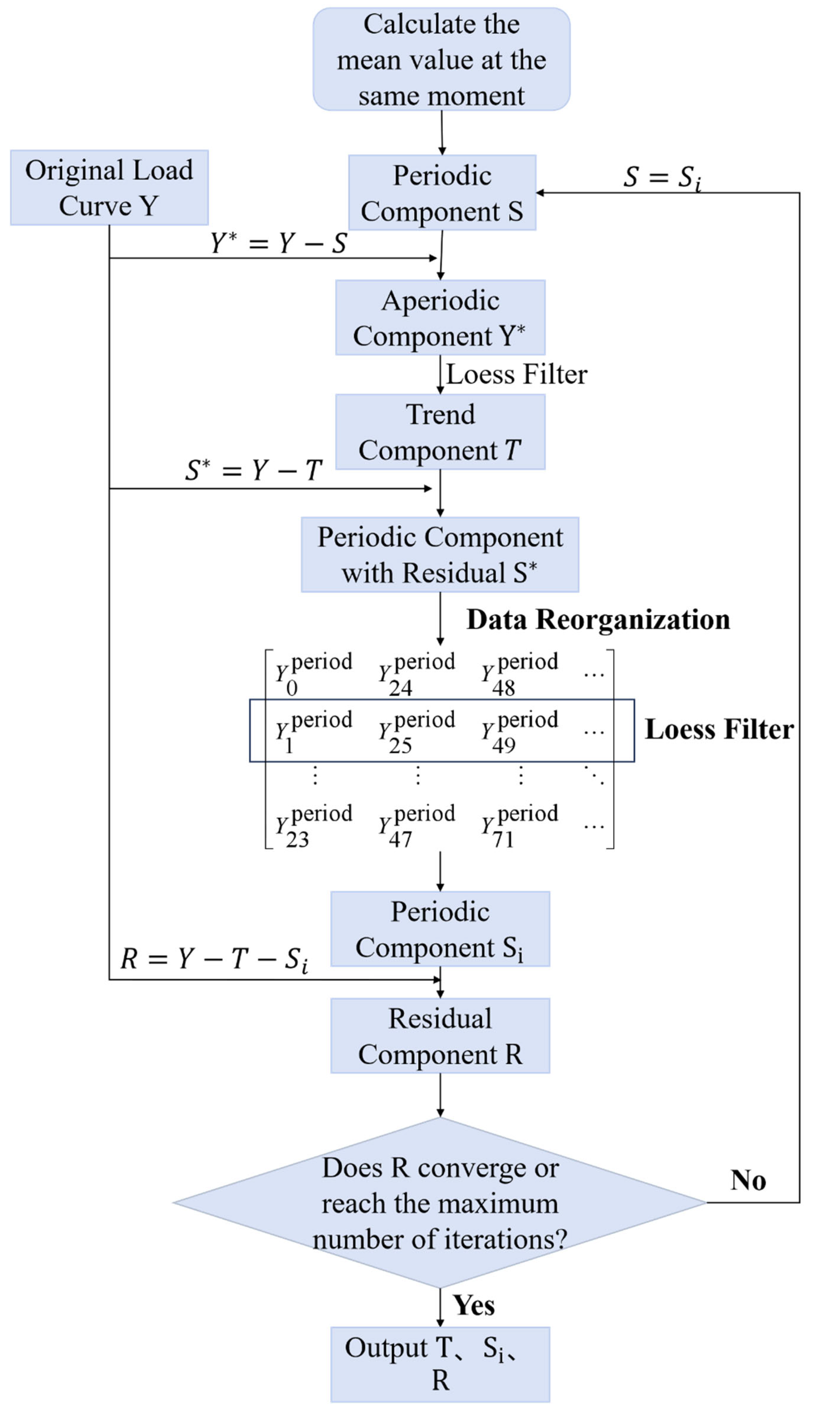
To address the characteristic differences in load across various time scales, the proposed method employs the STL algorithm to decompose the annual load into three components: trend, seasonal, and residual. The algorithm’s process is illustrated in Figure 2. As shown in the figure, an initial estimate of the seasonal component S is first calculated by averaging the original load values at the same time point across all days. This seasonal component is then subtracted from the original series Y to obtain the non-seasonal component Y * = Y S . A Loess smoothing filter is applied to Y * to extract the trend component T , and the seasonal residual S * = Y T is recalculated accordingly. The data is then reorganized based on the daily cycle, and another round of Loess smoothing is applied to derive an updated seasonal component, S i . The residual component is subsequently computed as R = Y T S i . This process is performed iteratively: if the residual R has not converged or the maximum number of iterations has not been reached, the algorithm continues updating. Once convergence is achieved or the iteration limit is reached, the final trend T , seasonal component S i , and residual component R   are output.
The core of STL lies in the iterative application of the locally estimated scatterplot smoothing (Loess) function to estimate each component. The seasonal period is set to 24 h. For each position within a period, the average value at that position is calculated to initialize the seasonal component, as expressed in the following formula:
S i ( 0 ) = 1 N i t i ( mod p ) Y t
N i denotes the number of samples at location i , and ( . ) represents the iteration count.
After removing the periodic component from the original data, we obtain
Y t * = Y t S t ( 0 )
Y t * is smoothed using Loess filtering. The core idea is to take a small neighborhood of data around each target point t 0 , construct a local low-order polynomial model, and then fit this model using weighted least squares to estimate the trend value at that point.
The T0 window is selected in the vicinity of t 0 , and the set of points within this window is denoted as follows:
{ ( t i , y i ) | t i neighborhood ( t 0 ) }
In the above equation, t i denotes adjacent time instants, and y i represents the corresponding load values. For each point t i , a weight w i is assigned based on its distance to t 0 , as expressed in the following formula:
w i = ( 1 ( t i t 0 d ) 3 ) 3
In the equation, d denotes one-half of the window width, ensuring that observations closer to t 0 receive larger weights and therefore exert a stronger influence during the fitting process. In this domain, a local quadratic model is employed to fit the trend at the point, with the formula defined as follows:
y i β 0 + β 1 ( t i t 0 ) + β 2 ( t i t 0 ) 2
The parameters β 0 , β 1 , and β 2 are estimated using the least squares method, with the objective function defined as follows:
min β 0 , β 1 , β 2 i neighborhood w i ( y i β 0 β 1 ( t i t 0 ) β 2 ( t i t 0 ) 2 ) 2
Substituting the regression outcome into t 0 , the trend value at that point is obtained as t 0 .
After obtaining the trend component T t , the residual component R t is derived by subtracting A from the annual load Y t . Subsequently, adding the residual component R t to the seasonal component S t yields Y t period , which represents the noisy seasonal component. This composite sequence is then reorganized as follows:
Y 0 p e r i o d Y 1 p e r i o d Y 23 p e r i o d Y 24 p e r i o d Y 25 p e r i o d Y 47 p e r i o d Y 48 p e r i o d Y 49 p e r i o d Y 71 p e r i o d
In the equation, each row represents the seasonal component at Y t period in the same position within a cycle. Loess smoothing is applied independently to each row; the resulting seasonal estimates are then re-assembled in chronological order to yield the updated component S t ( 1 ) , which subsequently replaces the corresponding entry S t ( 0 ) in the matrix X. This iterative procedure is repeated until the residual component R t converges or the maximum number of iterations is reached.

2.1.2. Improved DDPM

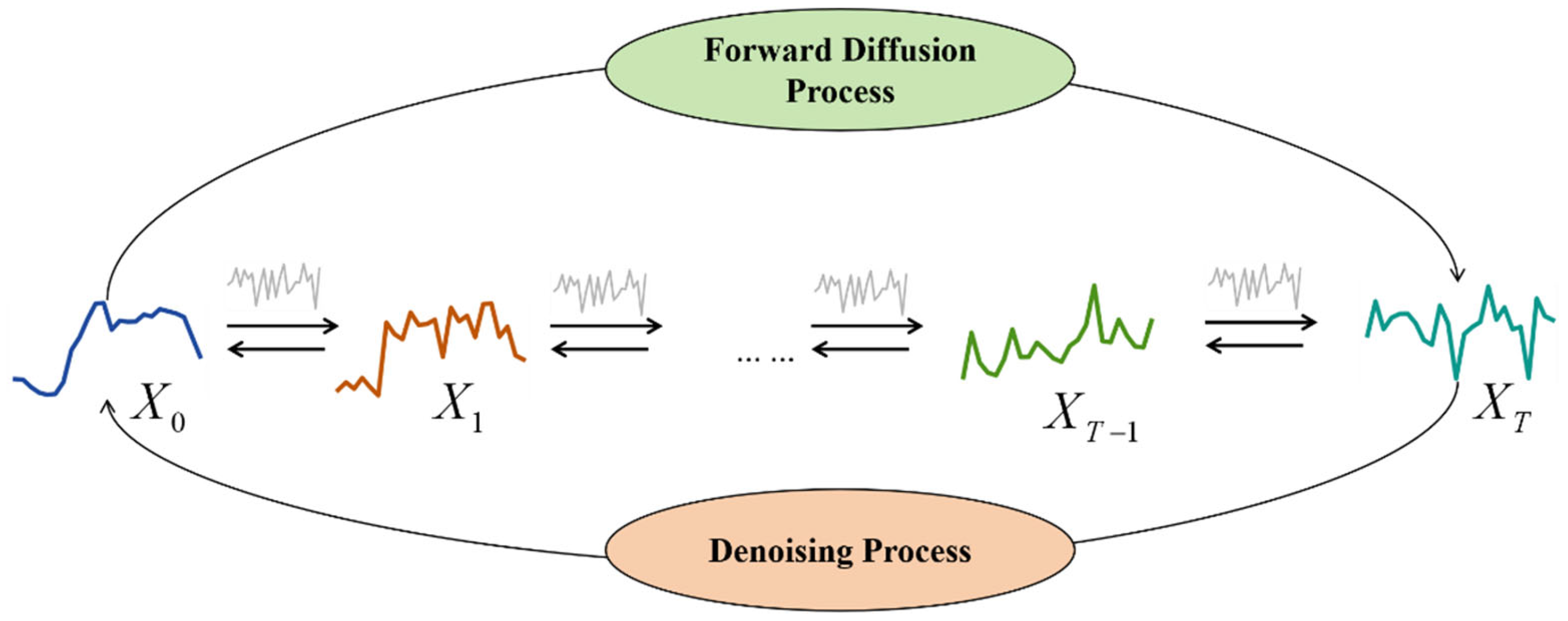
The DDPM consists of two processes: the forward diffusion process and the reverse denoising process. The overall procedure is illustrated in Figure 3. In the forward process, noise is gradually added to the original data until it converges to a Gaussian random distribution. At each diffusion step, a fixed amount of noise is injected, and the forward process can be defined as follows:
x t = 1 β t x t 1 + β t ε t
where x t denotes the diffusion state at time step t ; β t represents the noise variance at step t , which controls the intensity of the injected noise; and ε denotes Gaussian white noise.
The reverse denoising process aims to train the model to learn the denoising operation at each time step, thereby enabling scenario generation from random noise. However, conventional diffusion models lack the ability to control the generated samples. To address this issue, daily load profiles are classified into three categories: weekdays, holidays, and weekends. To achieve controllable generation with respect to load type, a conditional diffusion modeling approach is adopted to generate daily load components, and the corresponding formulation is given as follows:
p θ ( x t 1 | x t , c ) = N ( x t 1 ; μ θ ( x t , t , c ) , t )
where c denotes the conditioning variable, p θ ( x t 1 x t , c ) represents the reverse diffusion probability parameterized by θ and modeled by a neural network, μ θ ( x t , c , t ) denotes the conditional mean predicted by the denoising network, and Σ t denotes the covariance matrix of the reverse process at time step t .
To further enhance the model’s ability to discriminate among different types of samples, conditional information is incorporated into the residual blocks of the network. Through repeated utilization of these blocks, the influence of conditional information on the final sample generated is progressively strengthened.
The overall architecture of the proposed model is illustrated in Figure 1. The base structure adopts a U-Net framework, which consists of an encoder and a decoder with symmetric internal architectures connected through a bottleneck layer. In addition, the input time-series data are embedded into a 128-dimensional feature space at each time step, and positional encoding is applied to represent temporal order. The embedded features and positional encodings are summed to form the input representation. Notably, the positional encoding vectors are fixed and are not updated during model training.
In the processing of conditional information, a direct concatenation strategy is not employed to avoid information dilution. Instead, Feature-wise Linear Modulation (FiLM) is used to integrate conditional information into the network. The corresponding formulation is as follows:
( γ , β ) = MLP ( | Embed ( t ) , Embed ( c ) | ) FiLM ( h ) = γ ( t , c ) h + β ( t , c )
where h denotes the input features of the layer and γ ( c ) and β ( c ) represent the conditional scaling and shifting vectors, respectively. Both parameters are learnable and generated via a multilayer perceptron.
The training objective is to minimize the mean-squared error between the true noise ε and the predicted noise ε θ ( x t , t , c ) , which can be formulated as follows:
L ( θ ) = E t , x 0 , ϵ , c [ ϵ ϵ θ ( x t , t , c ) 2 ]
where 2 2 denotes the squared l 2 -norm, which is used to measure the discrepancy between the predicted noise and the true noise.

2.2. Evaluation Criteria

The generated load scenarios need to closely match the characteristics of the actual data. The generated scenarios are evaluated according to two aspects: time correlation and validity.

2.2.1. Time Relevance Metrics

This metric evaluates the model’s ability to capture temporal characteristics, verifying temporal consistency between generated and actual scenarios. An autocorrelation function (ACF) is employed as the assessment criterion and formulated as follows:
ACF ( k ) = t = 1 T k ( x t x ¯ ) ( x t + k x ¯ ) t = 1 T ( x t x ¯ ) 2
In the above equation, ACF ( k ) denotes the autocorrelation coefficient, k the time lag, x t the data at time t , and x ¯ the daily mean. The index ranges in [−1, 1]; values closer to 1 indicate stronger positive autocorrelation, values closer to −1 stronger negative autocorrelation, and a value of 0 implies no autocorrelation.
The kernel density estimate of the ACF coefficients at different lags is computed daily, and Kullback–Leibler (KL) divergence is employed to quantify the discrepancy between the generated and real samples in temporal correlation. Smaller KL divergence signifies that the temporal structure of the generated samples is close to that of the real data.

2.2.2. Effectiveness Indicator

Validity denotes the accuracy with which the generated scenarios characterize load uncertainty. In this study, validity is evaluated using three metrics: Pinball Loss, average power-interval width, and energy score (ES); the corresponding expressions are given below.
P i n b a l l = 1 M D m = 1 M d = 1 D [ τ max ( y d y ^ d m , 0 ) + ( 1 τ ) max ( y ^ d m y d , 0 ) ]
Equation (13) presents the Pinball Loss formula, where M denotes the number of generated samples, D denotes the temporal dimension of the samples, y d denotes the observed value at the d -th time step, y ^ d m denotes the m-th generated value at the d -th time step, and τ denotes the quantile parameter. This metric quantifies the accuracy of generated scenarios at a given quantile; a smaller value indicates higher coverage of the real scenario.
W = 1 T t = 1 T ( P t up P t down )
Equation (14) is the formula for the average width of the power interval, where P t up is the upper bound of the scenario set generated at time t , P t down is the lower bound of the scenario set generated at time t , and W is the average width of the power interval of the generated scenarios. A smaller W value indicates that the generated scenarios are closer to reality.
E S = 1 M i = 1 M x i y 1 2 M 2 i = 1 M j = 1 M x i x j
Equation (15) gives the ES metric, where x i denotes the i -th generated sample, y the real sample, M the number of generated samples, and . the L2-norm distance; the value decreases as the generated samples approach the real ones while simultaneously increasing in diversity.

3. Results and Discussion

The proposed method was validated using 8784 instances of hourly load data from a city in a southern Chinese province for the year 2024.

3.1. STL Decomposition of Load

In STL decomposition, the choice of filtering window plays a crucial role in determining the decomposition quality. A window that is too small may cause short-term fluctuations to be mixed into the trend component, resulting in residuals that still exhibit significantly structured patterns. Conversely, a window that is too large may lead to over-smoothing of the trend component, thereby obscuring actual medium- and long-term variation patterns.
To address this issue, a comprehensive evaluation metric is proposed that considers both the Reconstruction Error (RE) and the Trend Smoothness (TS) to guide the selection of an appropriate window size. The metric is defined as follows:
J = 1 N i = 1 N y i ( s ^ i + t ^ i ) 2 + 1 N 1 i = 2 N t ^ i t ^ i 1 2
where y i denotes the observed value of the original time series at time step i ; s ^ i and t ^ i represent the seasonal and trend components extracted via STL decomposition, respectively; and N is the total number of time steps in the series. The first term measures the reconstruction error, i.e., the average squared difference between the original series and the sum of its decomposed components. The second term reflects the smoothness of the trend component, quantified by the squared first-order difference. A lower value suggests that the decomposition achieves higher fidelity and smoother trend representation.
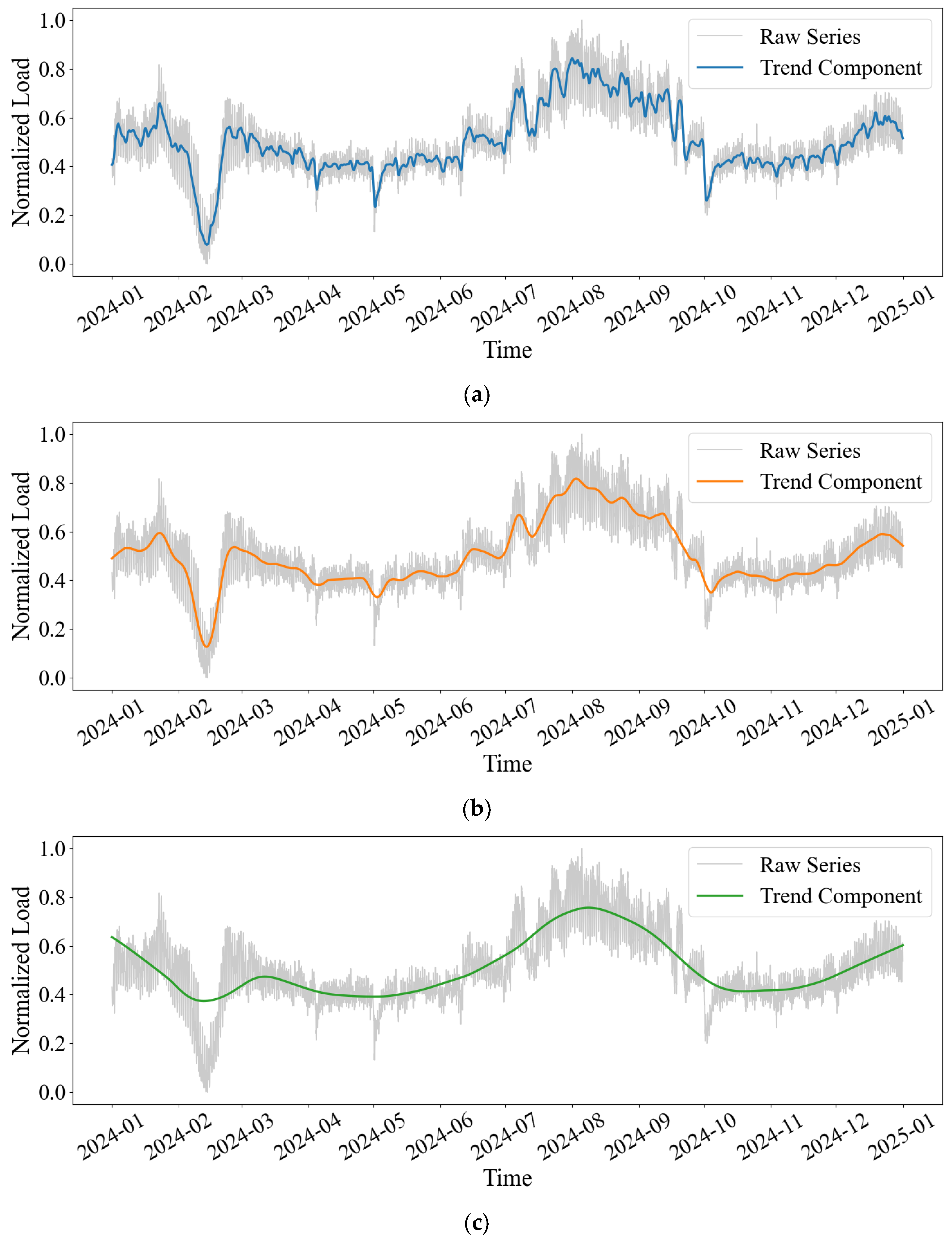
Since load data exhibit clear daily periodic fluctuations, the candidate filtering windows are set as integer multiples of 24 h, specifically including 24, 148, 720, and 1440 h. The composite evaluation indicators calculated under different windows are shown in Table 1. As shown in the results, when the window size is 720 h, the composite indicator reaches its minimum. Therefore, 720 was selected as the filtering window for STL decomposition.
To further illustrate the filtering effects under different window sizes, three representative windows—24, 148, and 720 h—were selected, and their corresponding trend components are plotted in Figure 4. This figure shows that as the window size increases, short-term fluctuations are gradually removed from the trend component. When the window is set to 720 h, the trend component captures only the long-term variation in the load on an annual time scale, demonstrating good smoothness and the preservation of meaningful long-term structures.

3.2. Improved DDPM

The improved DDPM is configured with 500 diffusion steps, an initial noise scale of 0.0001, and a terminal noise scale of 0.02. A U-Net architecture is adopted as the denoising network, with specific model parameters detailed in Table 2. During training, the Adam optimizer is employed with a learning rate of 0.0002 and a batch size of 32. All activation functions used in the model are SiLU. The embedding dimension for the diffusion time step is set to 128, while the embedding dimension for the conditional information is set to 64.
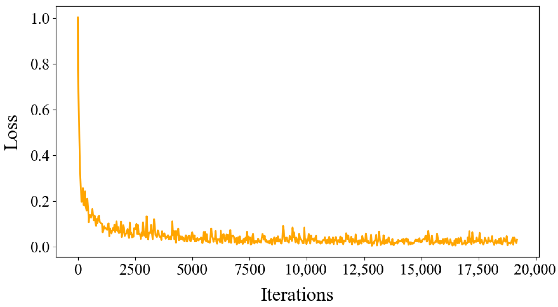
The load characteristics at the daily time scale are mainly influenced by the holiday schedule. The overall load level on weekends is lower than on weekdays, and the load level on holidays is even lower than on weekends. Based on this, daily load variation components are classified into three categories: weekdays, weekends, and holidays. These categories are distinguished using one-hot vectors as labels. The data are then input into the proposed model for training. The loss curve is shown in Figure 5; as shown in the figure, the proposed model converges quickly, and the training process is stable.
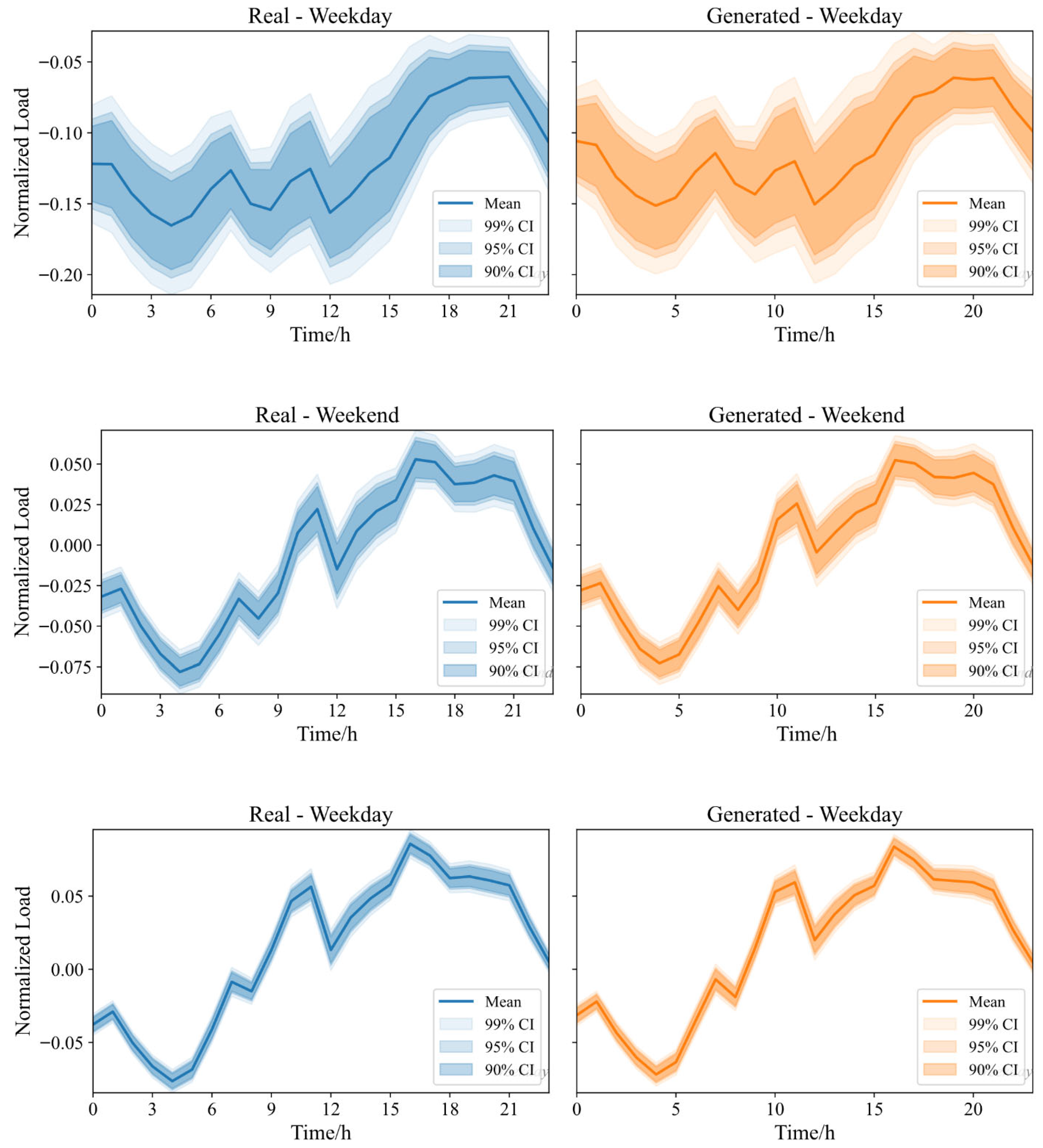
The generated daily load variation components for different types of loads are shown in Figure 6. As observed, the overall range of the generated load closely matches that of the corresponding real load, and the load variation trends are largely consistent. For instance, the daily load variation components on holidays generally remain below zero and exhibit no significant peaks or troughs within the day, and the generated holiday load components align well with these characteristics.
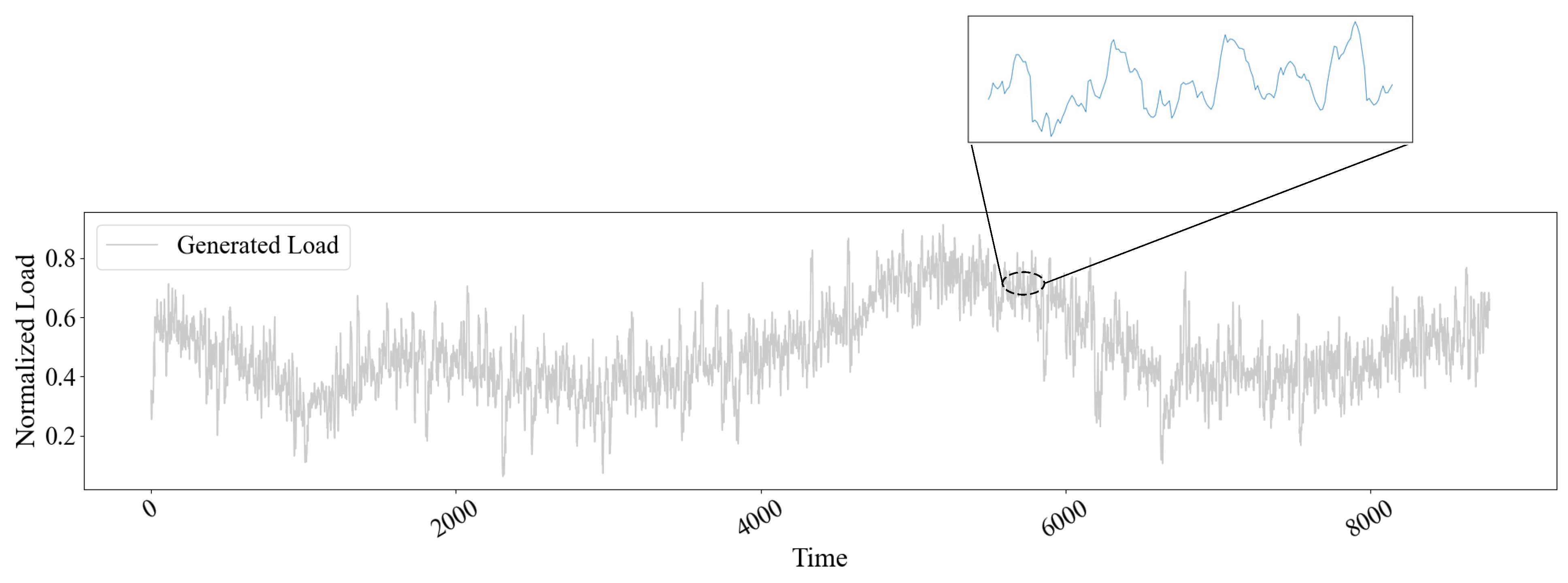
Using the decomposed load trend component as a baseline, the daily load variation components generated by type are added to the trend component hour by hour to construct the full-year load scenarios, as shown in Figure 7. In the figure, the generated annual load scenarios closely follow the overall variation trends of the real load data, effectively avoiding abnormal scenarios that contradict actual operational patterns. Meanwhile, at shorter time scales, the generated load curves capture reasonable temporal fluctuations and random perturbations, ensuring diversity and differences among various scenarios. This method maintains the authenticity of the annual load trend while introducing necessary randomness, achieving an effective balance between realism and variability in the full-year load scenarios.

3.3. Method Comparison

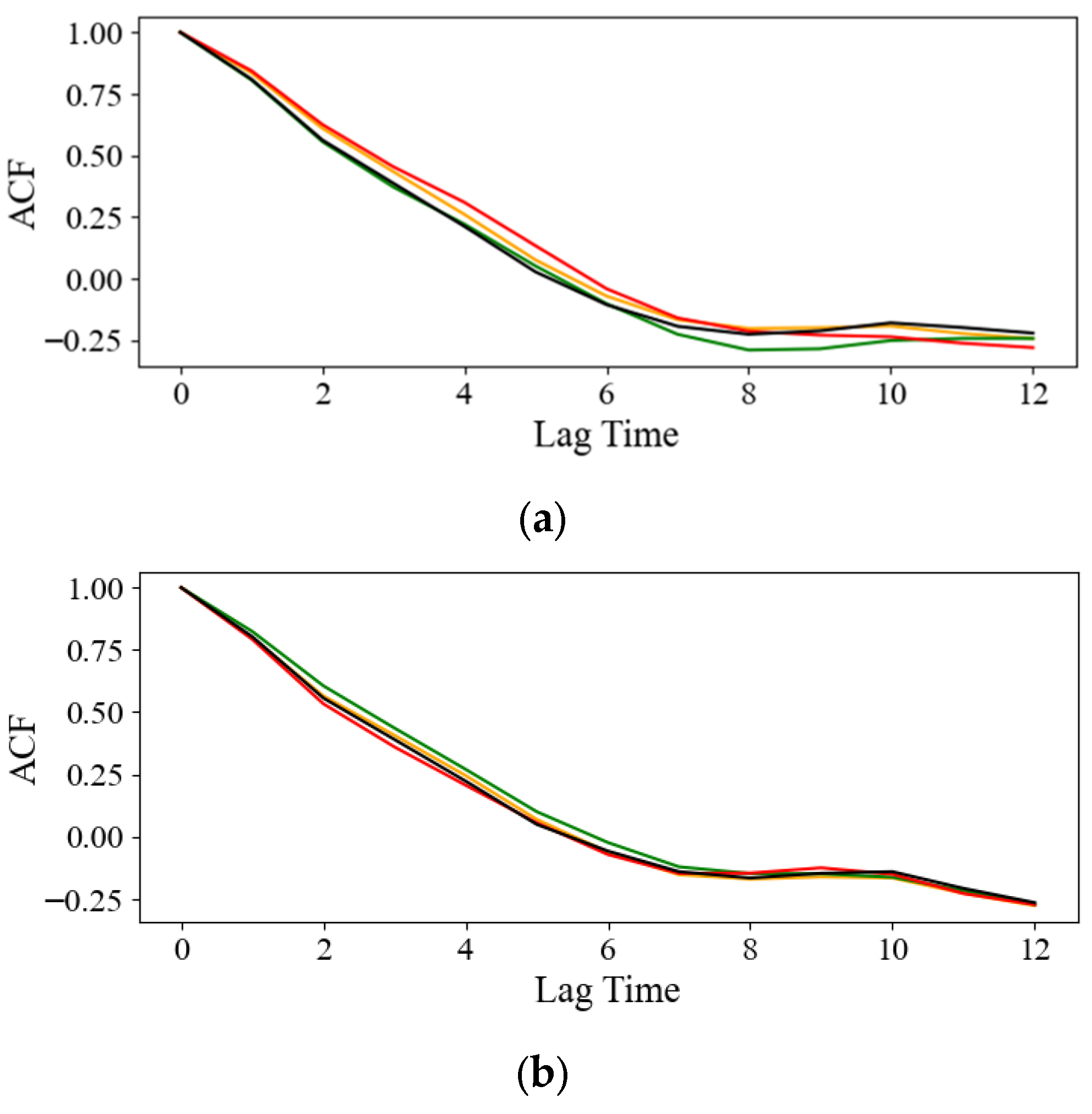
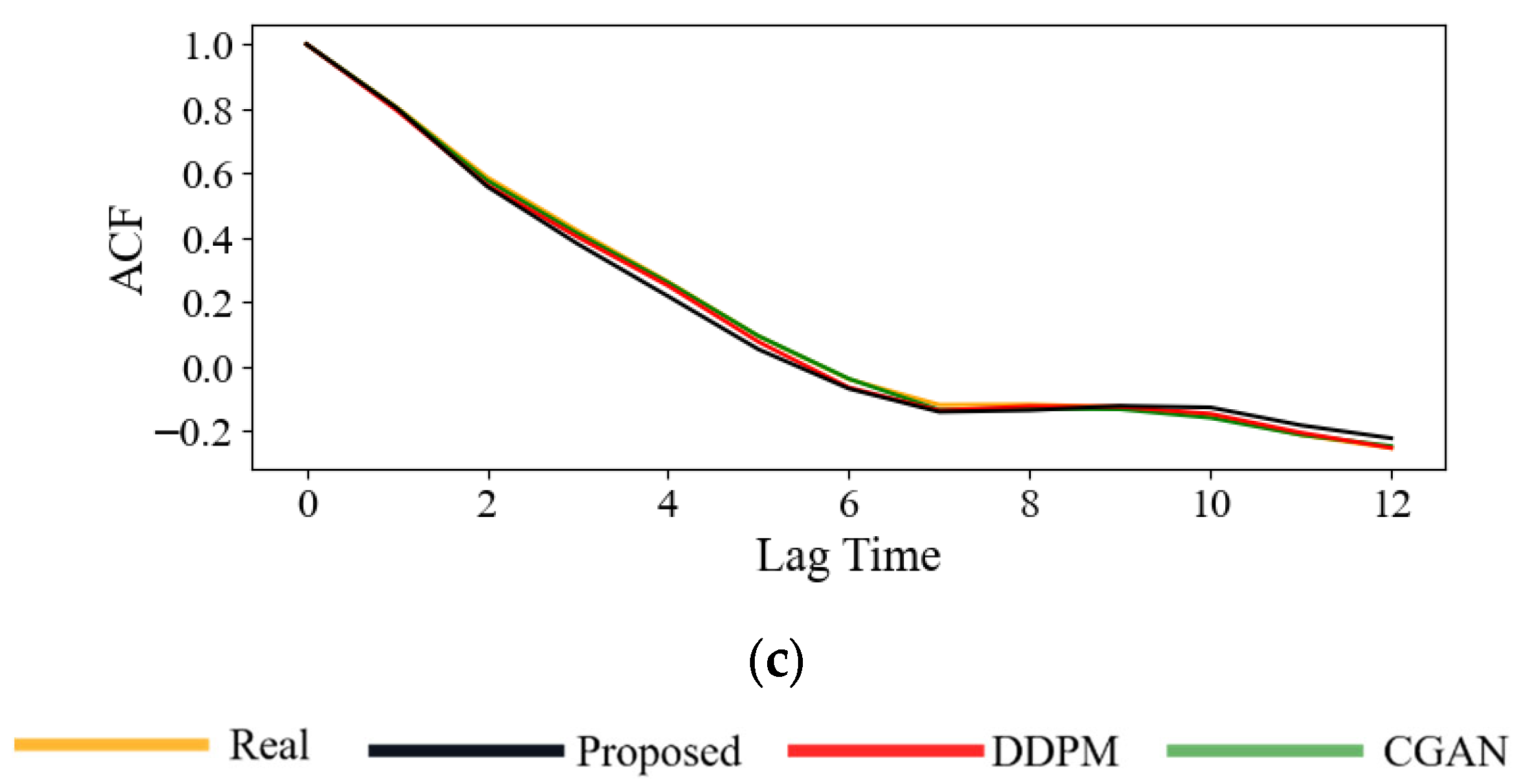
First, the daily scenario generation method proposed in this study is compared with CGAN and DDPM. As shown in Figure 8, the mean ACF coefficients of the scenarios generated by the different methods are close to the real values.
To further quantify the differences between methods, the Wasserstein distances between the ACF of the generated and real load curves at multiple lag steps were computed, and the mean Wasserstein distance and the corresponding variance across 12 lag points for each method were calculated based on these values. These metrics reflect the similarity and stability of the generated results in terms of temporal correlation. The results are presented in Table 3. As shown in the table, the DDPM method outperforms CGAN in terms of the ACF-based quantitative metrics across all three types of load scenario generation tasks. Building upon this, the proposed improved DDPM further enhances performance. Specifically, the Wasserstein distance of the ACF decreases by 7.2% for workdays, 9.2% for holidays, and 5.8% for weekends. These results demonstrate the superior capability of the proposed method in accurately capturing the temporal characteristics of load time series.
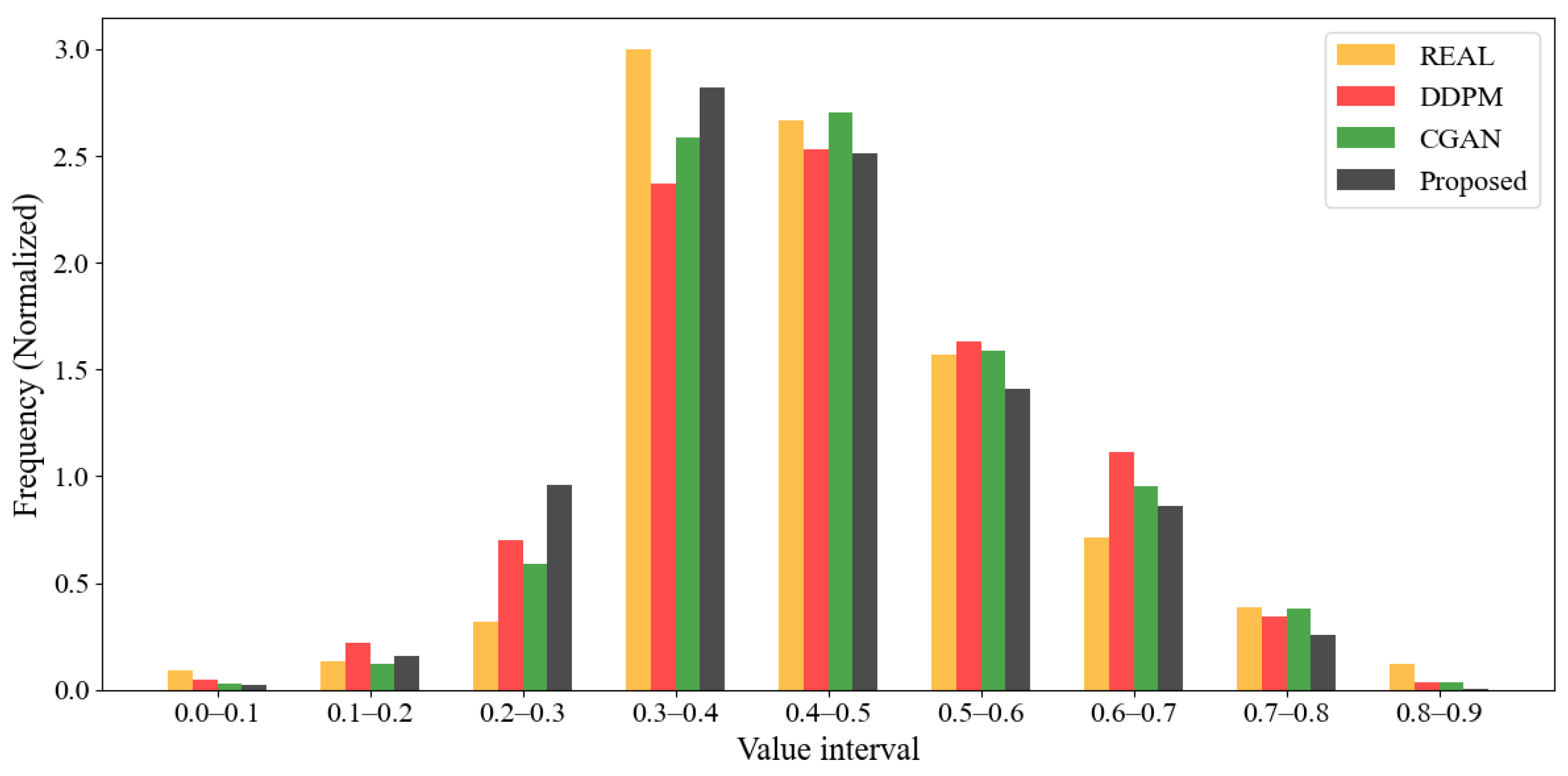
The load value ranges of the generated daily scenarios are illustrated in Figure 9, which shows that the range distributions of the scenarios generated by all methods are generally consistent with the real values. The KL divergence metric is further introduced to quantify the differences between distributions; the smaller the value, the closer the generated scenario distribution is to the real scenario. Specifically, the KL divergence of the proposed method is 0.242, while those of the CGAN and DDPM methods are 0.393 and 0.526, respectively. This indicates that the proposed method has an advantage in accurately representing the numerical characteristics of the generated scenarios.
The method proposed in this study integrates the STL algorithm with an improved DDPM for full-year load scenario generation. To further quantitatively evaluate the advantages of the proposed approach, the daily load generation method presented herein was combined with an existing annual scenario generation method, specifically the annual load scenario generation approach that integrates MCMC and the improved DDPM. Both methods were compared using the ES, Pinball Loss, and interval width as quantitative metrics to analyze the relative performance of the existing method and the proposed approach. The quantitative results are shown in Table 2. As observed, the annual load generated by the proposed method outperforms the comparison methods across all evaluated metrics. The ES metric is reduced by 28.2%. At the 90%, 95%, and 99% confidence levels, both the Pinball Loss and interval width show noticeable improvements, with the average Pinball Loss decreasing by 17.3% and the average interval width by 23%. The ES metric is defined as shown in Equation (15). The first term measures the consistency between the generated and real samples, where a lower value indicates higher consistency. The second term quantifies the diversity of the generated samples, where a higher value reflects stronger diversity.
In our proposed method, the consistency and diversity metrics are 1.503 and 0.612, respectively, while the corresponding values for the baseline method are 1.842 and 0.601. Overall, the proposed approach achieves better alignment with real samples while maintaining adequate diversity in the generated annual scenarios.

4. Conclusions

To address the issues with existing methods for generating annual load scenarios—namely insufficient trend representation capability over long time scales, excessive randomness in generated scenarios that deviates from reality, and inadequate consideration of special scenarios such as holidays—a method for generating the annual 8760 h load curve by integrating STL decomposition and improved DDPM is proposed. As shown in Table 4, the experimental results demonstrate that the proposed method outperforms the comparative approach across multiple quantitative evaluation metrics. The specific conclusions of this study are as follows:
  • The improved DDPM converges quickly during training, and the training process is stable. The generated daily load scenarios outperform existing CGAN and DDPM methods across various quantitative metrics, and the model demonstrates a clear advantage under small-sample conditions.
  • By combining STL decomposition with the improved DDPM, this study proposes a method for generating full-year load scenarios. This approach preserves the overall statistical characteristics and temporal structure of the load while introducing controlled random perturbations, thereby achieving a balance between realism and variability. Compared with traditional mid- to long-term load scenario generation methods, the generated annual load scenarios achieve superior results across multiple quantitative evaluation metrics.

Table 4. Quantitative evaluation metrics of generated curves.
Quantitative IndicatorConfidence IntervalMethod Proposed in This PaperComparison Methodp-Value
ES/0.8911.241/
Pinball Loss90%0.01090.0132<0.001
95%0.01070.0129<0.001
99%0.01050.0127<0.001
interval width90%0.140.19<0.001
95%0.160.20<0.001
99%0.170.22<0.001
The proposed method primarily focuses on generating load scenarios for normal years; systematic research has not yet been conducted on load evolution characteristics under extreme conditions, such as extreme high temperatures or natural disasters. This work can be further extended to the modeling and generation of extreme scenarios to enhance the method’s adaptability and robustness under abnormal operating conditions.

Author Contributions

Conceptualization, H.K. and H.L. (Haibo Li); methodology, X.W. and R.H.; software, J.L.; validation, H.K. and J.C.; formal analysis, W.H.; investigation, W.H.; resources, H.K. and H.L. (Liu Hongyang); data curation, X.W.; writing—original draft preparation, H.K. and R.H.; writing—review and editing, W.Y.; visualization, H.L. (Haibo Li); supervision, Z.L.; project administration, Z.L. All authors have read and agreed to the published version of the manuscript.

Funding

This research was funded by State Grid Inner Mongolia Eastern Electric Power Co., Ltd., grant number SGMDJY00GPJS2500008.

Data Availability Statement

The data presented in this study will be available when required.

Conflicts of Interest

Authors Heran Kang, Hongyang Liu, Jianfei Liu, Wenbo Hu, Jie Chen, and Wei Yue were employed by State Grid Inner Mongolia Eastern Electric Power Co., Ltd. The remaining authors declare that the research was conducted in the absence of any commercial or financial relationships that could be construed as a potential conflict of interest. The authors declare that this study received funding from State Grid Inner Mongolia Eastern Electric Power Co., Ltd. The funder was not involved in the study design, collection, analysis, interpretation of data, the writing of this article or the decision to submit it for publication.

References

  1. Lin, C.F.; Bie, C.H. Review of static modeling and quantitative analysis methods for uncertainties of new power systems. Autom. Electr. Power Syst. 2024, 48, 14–27. [Google Scholar]
  2. Mi, Y.; Lu, C.K.; Shen, J.; Yang, X.; Ge, L. Wind power extreme scenario generation based on conditional generative adversarial network. High Volt. Eng. 2023, 49, 2253–2263. [Google Scholar]
  3. Zhao, P.F.; Xu, X.Z.; Dong, X.C.; Gao, Y.; Sun, Y. An adaptive decision making approach for transmission expansion planning considering risk assessment of renewable energy extreme scenarios. IET Gener. Transm. Distrib. 2023, 17, 4107–4118. [Google Scholar] [CrossRef] [Scilit]
  4. Fang, H.L.; Li, D.H.; Peng, H.; Hou, H.; Chen, H.Y.; Fan, Z.; Su, Y. Distributed solar energy planning method based on internet plus. Proc. CSEE 2017, 37, 1316–1323. [Google Scholar]
  5. Motlagh, O.; Berry, A.; O’Neils, L. Clustering of residential electricity customers using load time series. Appl. Energy 2019, 237, 11–24. [Google Scholar] [CrossRef] [Scilit]
  6. Li, B.; Sun, J.J.; Yu, P. A multi-dimensional typical scenarios generation algorithm for distribution network based on load clustering and network structure equivalence. Proc. CSEE 2021, 41, 2661–2670. [Google Scholar]
  7. Qu, K.; Li, P.; Huang, Y.H.; Si, G. Modeling and scenario generation method of annual load series for evaluation of renewable energy accommodation capacity. Autom. Autom. Electr. Power Syst. 2021, 45, 123–131. [Google Scholar]
  8. Tian, Y.F.; Xu, M.; Shi, Y.F.; Qiao, Y.; Wu, L.L. Scenario generation method of medium- and long-term load series considering meteorological factors. J. Glob. Energy Interconnect. 2024, 7, 715–725. [Google Scholar]
  9. Zeng, S.; Ding, Q.F.; Li, X.L.; Bai, J.; Ma, L.; Chen, P.; Jiao, R.; Yang, T. Scenario generation of air conditioning loads in buildings based on conditional TimeGAN. Power Syst. Technol. 2022, 46, 2448–2456. [Google Scholar]
  10. Li, J.B.; Chen, Z.Q.; Cheng, L.; Liu, X. Energy data generation with Wasserstein deep convolutional generative adversarial networks. Energy 2022, 257, 124694. [Google Scholar] [CrossRef] [Scilit]
  11. Wang, Q.; Zhang, X.G.; Xu, D.G. Source-load scenario generation based on weakly supervised adversarial learning and its data-driven application in energy storage capacity sizing. IEEE Trans. Sustain. Energy 2023, 14, 1918–1932. [Google Scholar] [CrossRef] [Scilit]
  12. Huang, N.T.; Wang, W.T.; Cai, G.W.; Yang, D.; Huang, D.; Song, X. The joint scenario generation of multi source-load by modular denoising variational autoencoder considering the complex coupling characteristics of meteorology. Proc. CSEE 2019, 39, 2924–2934. [Google Scholar]
  13. Luo, P.P.; Sheng, A.; Lin, J.K.; Ma, Q.; Xu, Q.; Liu, Y.M. Scenario generation method of typhoon meteorological load based on interpretability. Autom. Electr. Power Syst. 2025, 49, 186–197. [Google Scholar]
  14. Xiao, B.; Huang, Y.R.; Jiang, Z.; Shi, Y.; Jiao, M.; Wang, Y. The method of spatial load forecasting based on the generative adversarial network for data scarcity scenarios. Proc. CSEE 2020, 40, 7790–8001. [Google Scholar]
  15. Huang, J.J.; Zhao, P.F.; Zhou, H.; Xu, X.; Gao, Y.; Sun, Y. Medium- and long term time-series scenarios generation based on typical source-load coupling modes. J. Glob. Energy Interconnect. 2024, 7, 271–282. [Google Scholar]
  16. Wu, X.; Xu, K.; Hall, P. A survey of image synthesis and editing with generative adversarial networks. Tsinghua Sci. Technol. 2017, 22, 660–674. [Google Scholar] [CrossRef] [Scilit]
  17. He, S.; Liao, W.; Yang, M.Y.; Yang, Y.; Song, Y.-Z.; Rosenhahn, B.; Xiang, T. Context-aware layout to image generation with enhanced object appearance. In Proceedings of the 2021 IEEE/CVF Conference on Computer Vision and Pattern Recognition (CVPR), Nashville, TN, USA, 20–25 June 2021; pp. 15049–15058. [Google Scholar]
  18. Yang, C.; Shen, Y.; Zhou, B. Semantic hierarchy emerges in deep generative representations for scene synthesis. Int. J. Comput. Vis. 2021, 129, 1451–1466. [Google Scholar] [CrossRef] [Scilit]
  19. Azadi, S.; Pathak, D.; Ebrahimi, S.; Darrell, T. Compositional gan: Learning image-conditional binary composition. Int. J. Comput. Vis. 2020, 128, 2570–2585. [Google Scholar] [CrossRef] [Scilit]
  20. Zhao, W.; Shao, Z.; Yang, S.; Lu, X. A novel conditional diffusion model for joint source-load scenario generation considering both diversity and controllability. Appl. Energy 2025, 377, 124555. [Google Scholar] [CrossRef] [Scilit]
  21. Dong, X.; Sun, Y.; Yang, Y.; Mao, Z. Controllable renewable energy scenario generation based on pattern-guided diffusion models. Appl. Energy 2025, 398, 126446. [Google Scholar] [CrossRef] [Scilit]
  22. Li, S.; Xiong, H.; Chen, Y. DiffPLF: A conditional diffusion model for probabilistic forecasting of EV charging load. Electr. Power Syst. Res. 2024, 235, 110723. [Google Scholar] [CrossRef] [Scilit]
  23. Bayode, I.A.; Ba-Alawi, A.H.; Nguyen, H.T.; Woo, T.; Yoo, C. Long-term policy guidance for sustainable energy transition in Nigeria: A deep learning-based peak load forecasting with econo-environmental scenario analysis. Energy 2025, 322, 135707. [Google Scholar] [CrossRef] [Scilit]
  24. Zheng, W.; Chen, Z.; Zheng, K.; Zheng, W.; Chen, Y.; Fan, X. WorkloadDiff: Conditional Denoising Diffusion Probabilistic Models for Cloud Workload Prediction. IEEE Trans. Cloud Comput. 2024, 12, 1291–1304. [Google Scholar] [CrossRef] [Scilit]
  25. Li, S.; Xiong, H.; Chen, Y. Diffcharge: Generating ev charging scenarios via a denoising diffusion model. IEEE Trans. Smart Grid 2024, 15, 3936–3949. [Google Scholar] [CrossRef] [Scilit]
  26. Yao, T.; Liu, C.; Wang, Y.; Zhou, F.; Chen, X.; Chai, B.; Zhang, W.; Wan, Z. Weather-Informed Load Scenario Generation Based on Optical Flow Denoising Diffusion Transformer. IEEE Trans. Smart Grid 2025, 16, 4225–4236. [Google Scholar] [CrossRef] [Scilit]
  27. Ma, W.; He, G.; Che, L. Conditional denoising diffusion probabilistic model based ante-hoc explainable scenario generation for power systems dispatch. Energy 2025, 332, 137115. [Google Scholar] [CrossRef] [Scilit]
  28. Dou, X.; Niu, P.Y.; Zheng, Y.X.; Feng, S.; Shi, F.; Yang, H. Scenario generation method covering extreme form load based on improved diffusion model. Proc. CSEE 2024, 45, 9152–9164. [Google Scholar] [CrossRef]
  29. Gao, Y.; Yang, H.J.; Guo, K.J.; Ma, Y. Optimal pricing strategy of electricity price demand response considering seasonal characteristics of load. Electr. Power Constr. 2023, 44, 55–63. [Google Scholar]
  30. Cleveland, R.B.; William, S.; Jean, E.M.; Terpenning, I. STL: A seasonal-trend decomposition procedure based on loess. J. Off. Stat. 1990, 6, 3–73. [Google Scholar]
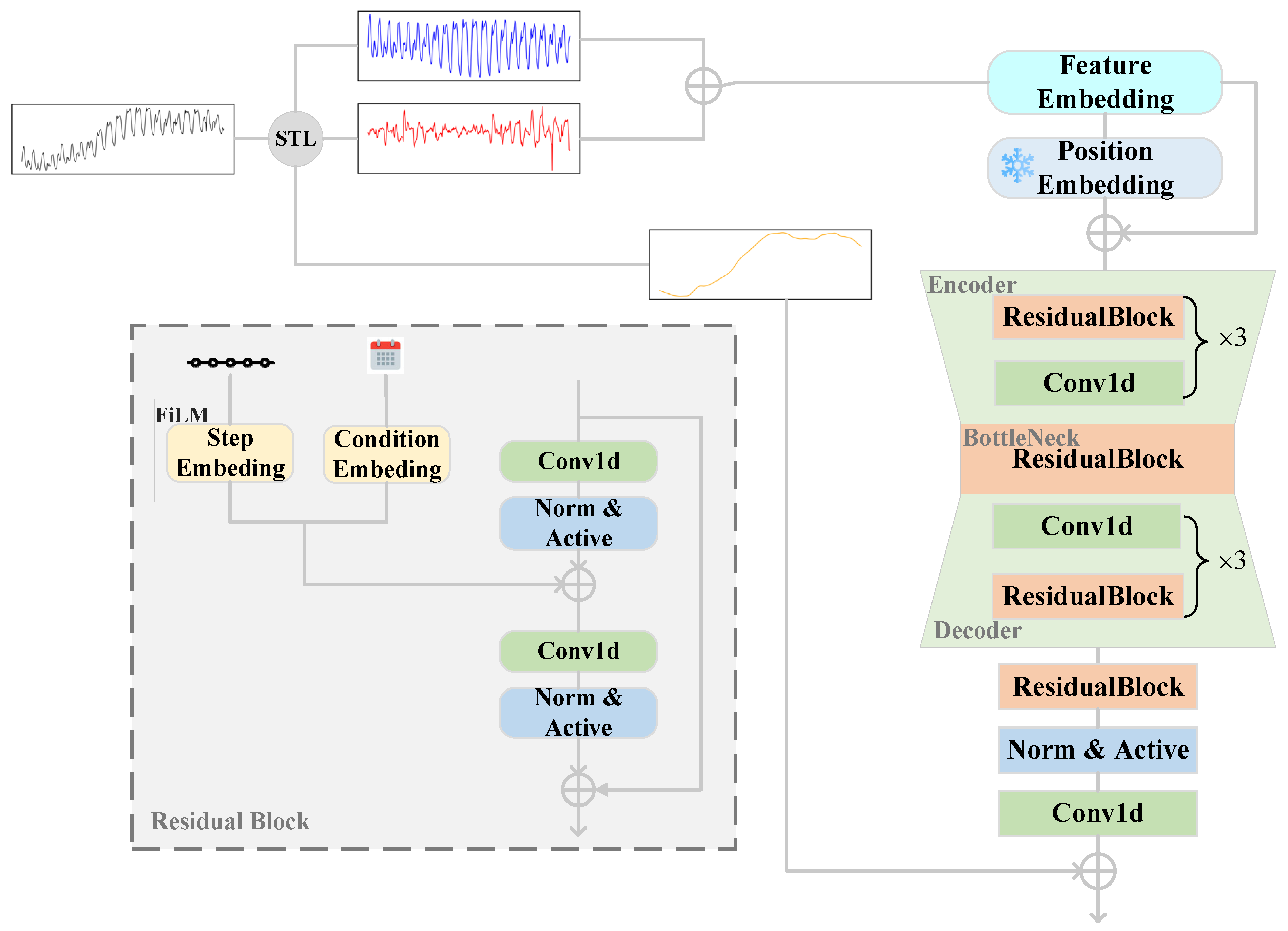
Figure 1. Annual load scenario generation flowchart.
Inventions 11 00021 g001
Figure 2. STL algorithm flowchart.
Inventions 11 00021 g002
Figure 3. Illustration of the DDPM forward diffusion and denoising processes.
Inventions 11 00021 g003
Figure 4. Illustration of trend component extraction under different STL window sizes. (a) Trend component extracted with a 24 h STL window; (b) Trend component extracted with a 148 h STL window; (c) Trend component extracted with a 720 h STL window.
Inventions 11 00021 g004
Figure 5. Illustration of the training loss curve.
Inventions 11 00021 g005
Figure 6. Illustration of the mean and confidence interval ranges for real and generated daily scenarios under different types.
Inventions 11 00021 g006
Figure 7. Illustration of the generated annual load curve. The gray line represents the entire annual curve, while the blue line highlights the zoomed-in section of the curve.
Inventions 11 00021 g007
Figure 8. Average ACF curves of different scene types generated by various methods and real scenarios. (a) Holiday average ACF curve; (b) Weekend average ACF curve; (c) Weekday average ACF curve.
Inventions 11 00021 g008aInventions 11 00021 g008b
Figure 9. Range distribution of real scenarios and those generated by different methods.
Inventions 11 00021 g009
Table 1. Evaluation index table for STL window size selection.
Window Size241487201440
Composite Evaluation Index1.060.840.721.00
Table 2. Architecture of U-Net in DDPM.
StageLayerChannels (In → Out)Length
InputConv1D1 → 6424
Encoder1Residual Block64 → 6424
Downsample Conv64 → 6412
Encoder2Residual Block64 → 12812
Downsample Conv128 → 1286
Encoder3Residual Block128 → 1286
Downsample Conv128 → 1283
BottleneckResidual Block128 → 1283
Decoder1Transposed Conv128 → 1286
Residual Block128 → 1286
Decoder2Transposed Conv128 → 12812
Residual Block128 → 6412
Decoder3Transposed Conv64 → 6424
Residual Block64 → 6424
FinalResidual Block64 → 6424
OutputConv1D64 → 124
Table 3. Wasserstein distance of different methods (mean + standard deviation).
WeekdayHolidayWeekend
CGAN0.0289 ± 0.01020.0604 ± 0.02510.0391 ± 0.0126
DDPM0.0195 ± 0.00590.0466 ± 0.01470.0260 ± 0.0123
Proposed0.0181 ± 0.00680.0423 ± 0.01030.0245 ± 0.0074
Disclaimer/Publisher’s Note: The statements, opinions and data contained in all publications are solely those of the individual author(s) and contributor(s) and not of MDPI and/or the editor(s). MDPI and/or the editor(s) disclaim responsibility for any injury to people or property resulting from any ideas, methods, instructions or products referred to in the content.