Time-Series Forecasting Patents in Mexico Using Machine Learning and Deep Learning Models

Abstract

Patenting is essential for protecting intellectual property, fostering technological innovation, and maintaining competitive advantages in the global market. In Mexico, strategic planning in science, technology, and innovation requires reliable forecasting tools. This study evaluates computational models for predicting applied and granted patents between 1990 and 2024, including statistical (ARIMA), machine learning (Regression Trees, Random Forests, and Support Vector Machines), and deep learning (Long Short-Term Memory, LSTM) approaches. The workflow involves historical data acquisition, exploratory analysis, decomposition, model selection, forecasting, and evaluation using the Root Mean Square Error (RMSE), the determination coefficient ($R^2$), and the Mean Absolute Percentage Error (MAPE) as performance metrics. To ensure generalization and robustness in the training stage, we use the cross-validation rolling origin. On the test stage, LSTM achieves the highest accuracy (RMSE = 106.91, $R^2=0.97$, and MAPE = 0.63 for applied patents; RMSE = 283.20, $R^2=0.93$, and MAPE = 2.65 for granted patents). However, cross-validation shows that ARIMA provides more stable performance across multiple scenarios, highlighting a trade-off between short-term accuracy and long-term reliability. These results demonstrate the potential of machine learning and deep learning as forecasting tools for industrial property management.

1. Introduction

Patents and inventions are fundamental drivers of economic and technical progress. Patenting is the legal process by which innovators are granted exclusive rights to manufacture and commercialize their ideas for a particular period of time [1]. A patent must meet three fundamental criteria, novelty, originality, and industrial applicability, providing a new and useful solution to a technical problem [2]. The number of patents granted indicates the ability of a country to innovate, create knowledge, and protect intellectual property [3,4]. A solid patent system promotes legal certainty, attracts investment, and improves competitiveness [5]. The WIPO Global Innovation Index ranks countries based on their innovation performance. This ranking considers technological progress, socioeconomic impacts, and investment in science and technology [6].

Mexico is the second-largest economy in Latin America after Brazil. It attracts foreign investment due to its stable macroeconomic conditions and strong integration with North American supply chains. This is particularly true in the automotive, electronics, aerospace, and medical device sectors [7,8]. Despite this economic strength, the country faces persistent challenges in innovation and patenting. After inactivity in the 1990s, patent activity showed some recovery, reaching 16,605 applications by 2022 [6]. However, the growth in patents does not align with the increase in gross domestic product (GDP), and Mexico still has a low patent density compared to other Organization of Economic Cooperation and Development (OECD) countries. This limits its global visibility of global innovation [9]. Furthermore, public patent databases, such as those of the Mexican Institute of Industrial Property (IMPI) [10], are underused because advanced predictive analytics have not yet been applied systematically to support innovation policy and technological development.

Patent data forecasting is essential for understanding technological development, which guides research, strategic planning, market analysis, and policy making. Predicting the number of patents in a country is complex due to the many factors that influence innovation [11]. Common approaches include historical trend analysis, economic modeling, sector analysis, public policy evaluation, and comparative analysis. Although no single method is ideal, the integration of multiple strategies with reliable data increases the accuracy of the forecast [12]. A key technique is time-series patent forecasting (TSPF), which analyzes past patent data such as applications, grants, or citations to predict future trends [13,14]. TSPF uses statistical models including ARIMA, exponential smoothing, and regression, as well as advanced machine learning, deep learning, and transformer-based methods, to capture complex patterns in technological evolution [15].

Recently, several works have studied time-series forecasting patents using a machine learning approach. For example, ref. [16] sets up a machine learning strategy to detect new innovations early using a dataset patent indicator that can be established as soon as relevant patents are granted. In [17], the authors reported a novel deep learning framework to predict the outcome of patent applications. Using a real-world dataset from the United States Patent and Trademark Office (USPTO), they achieved a predicting rate of 75%. Similarly, using LSTM, Zhang and Wang proposed a patent prediction scheme to predict rail transportation patents, showing a significant improvement relative to traditional models such as ARIMA [18]. In 2024, Tsai introduced a homogeneous forecasting model based on the hybrid imputation method. This model was used to predict the number of national patent applications and outperformed methods such as Random Forests, CNNs, and LSTM [19]. Ultimately, the use of Bi-LSTM in conjunction with optimization metaheuristics (the Alpine Skiing Optimization approach) to improve the classification and pre-selection of patents before forecasting achieves accuracies above 88% [20].

Although TSPF has advanced, issues remain. These challenges involve data heterogeneity, complexity, noise and uncertainty in time series, applicability between domains and between countries, prediction horizon, technological obsolescence, and decision-focused evaluations [21]. Unlike other countries that use patent prediction models with methods such as recurrent neural networks (RNNs), decision trees, or natural language processing (NLP) in application texts, Mexico lacks formal studies combining these approaches with national databases.

This study addresses the following research question:

RQ1. Which statistical model (ARIMA), machine learning (RT, RF, or SVM) or deep learning (LSTM), achieves the highest precision in forecasting time series of patent applications and grants in Mexico?

To answer this question, this study applies machine learning and deep learning algorithms using official historical patent data from 1993 to 2024. The objective is to develop reliable forecasting models for both applied and granted patents. This will provide a better understanding of the dynamics of Mexican technological innovation. Beyond model comparison, this work contributes by providing a quantitative framework that supports evidence-based policy making in science, technology, and innovation. It also highlights the potential of data-driven approaches to improve the strategic planning and evaluation of national innovation systems.

2. Materials and Methods

Analyzing time-series patent data requires a systematic approach that integrates various techniques to understand, model, and forecast data points collected over time [22]. Figure 1 shows the workflow for the forecasting of time-series patents.

2.1. Exploratory Data Analysis

The dataset used in this study was obtained from the Instituto Mexicano de la Propiedad Industrial through its open data platform (https://www.gob.mx/impi/documentos/instituto-mexicano-de-la-propiedad-industrial-en-cifras-impi-en-cifras) (accessed on 7 November 2025) and the Industrial Property Gazette System (SIGA) 2.0 [23], which provides public access to structured information on patent applications and granted patents in Mexico [24]. The dataset includes information from 1993 to Q2 of 2025, including variables such as the patent number, application date, publication date, applicant, International Patent Classification (IPC) code, and legal status. Since the IMPI and SIGA 2.0 systems are official repositories maintained under internal data quality protocols, no missing values were identified in the selected variables. The patent dataset is available online at https://docs.google.com/spreadsheets/d/11DJblFCsGsH_PxKFambn3uxF289r7l3w/edit?gid=1930750129#gid=1930750129 (accessed on 7 November 2025). We specifically use the following information from the dataset: invention applications, applications approved, and titles and registrations issued (1993–2024) (Inv 1); patents granted by technological field since 1993 to 2024 (Inv 7); and patents granted to Mexican holders by technological field (1993–2024) (Inv 8). For our applied and granted forecasting approach, the patent data in (Inv 1) include 32 instances that correspond to the annual measures of patents granted between 1993 and 2024. We did not consider 2025, since the dataset only contains information for the first quarter of the year.

Exploratory data analysis involves gathering observations over a specified period. This stage includes pre-processing and visualization tasks to prepare and understand the dataset for analysis and modeling, including data cleaning, data transformation, and structural operations [25]. Taking into account the characteristics of the dataset, a basic pre-processing step was applied. The pre-processing task used in this study was data normalization, in which each feature was divided by its maximum value for scaling purposes, resulting in values between 0 and 1. This normalization procedure ensured that all variables contributed proportionally to the learning process while preserving their original distribution patterns.

2.2. Decomposition

Decomposition is a technique used to analyze and interpret time-series data. This involves dividing the patent data into its fundamental components: trends, seasonal, cyclical, and remainder [26]. We use a function based on singular spectrum analysis (SSA) to find long-term trends, seasonality, and the remainder of the time-series patent data. SSA is a useful algorithm when periods of seasonal trends are unknown [27]. In time-series analysis, the remainder or irregular component represents the unpredictable ups and downs in a series that cannot be explained by trend, seasonal, or cyclical patterns. At this stage, a normality test was applied to the raw patent data only to determine whether the series followed a normal distribution before modeling. To this end, the Kolmogorov–Smirnov test was used to evaluate the normality of raw patent data [28].

2.3. Model Selection and Fitting

Based on attributes such as seasonality, trend, and stationary, model selection determines which model best captures the underlying patterns in the data. To ensure that the chosen model generalizes effectively to new data, the focus of model fitting is on training it to minimize the discrepancy between the observed data and predictions. Traditional forecasting models, machine learning models, and deep learning models are three popular methods for modeling time-series data.

The models selected for patent forecasting in this work represent a combination of traditional and modern forecasting techniques. ARIMA was used as a classical statistical benchmark, while Regression Trees, the Random Forest, and the SVM were chosen for their ability to model non-linear relationships [29]. The LSTM network was included due to its ability to capture long-term dependencies in sequential data [30,31]. These techniques are widely used in the literature as reference methods for forecasting tasks in several areas [32,33,34]. The following is a brief description of the models used.

2.3.1. ARIMA

ARIMA is a statistical time-series model that combines three components: autoregressive (AR), integrated (I), and moving average (MA). The current value depends on previous errors in the model. Its advantages include good performance in short-term forecasts when the series is relatively stable and clear statistical interpretation. However, its limitations lie in the fact that it does not handle structural changes, as well as the fact that it does not easily capture non-linearities or external effects if they are not incorporated [35].

2.3.2. Regression Tree

Regression analysis and sum of squares are used by an RT, a sort of decision tree, to forecast the values of the target field. It serves as a prediction model, since it is a non-parametric supervised learning technique for regression tasks. In this case, we use the binary decision tree fit for the regression model [36,37].

2.3.3. Random Forest

To increase the prediction accuracy in time-series analysis, the models construct multiple decision trees and add their output. These models avoid overfitting and can manage huge, high-dimensional datasets. They are ideal for modeling irregular patterns because they capture non-linear links and interactions by using historical data as predictors [38].

2.3.4. Support Vector Machines (SVMs)

The support vector machine model can handle high-dimensional data and describe non-linear interactions in time-series analysis, particularly with small and complex datasets [39].

2.3.5. Long Short-Term Memory

These models are a specific kind of recurrent neural network (RNN) that uses memory cells and gating techniques to overcome the drawbacks of conventional RNNs. Due to their ability to efficiently capture long-term dependencies, LSTM models are useful for time-series analysis applications such as sequence prediction and forecasting [17].

2.4. Model Prediction and Forecasting

The model that was trained in the previous stage is applied to new data for model prediction and forecasting, generating future data points based on past patent data. For training, we use the first 80% of the data, and for the prediction stage of the applied and granted patents, we use the remaining 20% [40]. Similarly, for a robust evaluation of the time series, we used cross-validation with an expanding window to select hyperparameters and compare models [41]. In this sense, we use a number of lags as predictors ($p=3$), an initial training size of 15, 10 iterations, and a one-step horizon ($h=1$).

2.5. Model Evaluation

Evaluating a model involves assessing its performance by metrics and quantifying the accuracy of its predictive capability. RMSE is one of the most widely used metrics; it computes the discrepancies between the predicted and actual values [42]. As an additional evaluation measure, the determination coefficient $R^2$ is a statistical metric widely used in the evaluation of forecasting models. $R^2$ measures the proportion of variability in the number of patents applied and granted per year that is explained by the forecasting model [43]. Additionally, MAPE is commonly used to measure prediction accuracy due to its interpretability and scale independence [44]. In this study, RMSE, $R^2$, and MAPE were used as evaluation metrics.

Different hyperparameters were explored and evaluated automatically by Bayesian optimization. This hyperparameter optimization algorithm was selected due to its ability to avoid unnecessary evaluations based on historical optimization values, as well as the use of a surrogate model, which enables a fast convergence speed for continuous hyperparameters [45,46]. The optimizer tuned the models until the best performance configuration was reached for each algorithm. The optimal ARIMA model was identified through an automatic grid search of various combinations of parameters of the autoregressive order component (p), the degree of differentiation (d), and the moving average component (q). The model with the lowest Akaike information criterion (AIC) was selected as the best-fitting configuration.

Table 1. Hyperparameter values for applied forecasting patents in the test stage.

Models	Optimized Hyperparameters
ARIMA	Order of the autoregressive component (p = 3), degree of differentiation (d = 1), and order of the moving average component (q = 3)
Regression trees	Minimum leaf size = 4, maximum number of splits = 24, minimum parent size = 10, and split criterion = mse
Random forest	Kernel function = linear, kernel scale = 1, epsilon = 0.0115, and solver = SMO
Support vector machines	Method = Bag and number of learning cycles = 10
Long short-term memory	One LSTM layer with number of hidden units = 16, dropout layer = 0.2776, and fully connected layer = 1. Training options: solver name = adam, maximum epochs = 686, gradient threshold= 1, initial learn rate = 0.0951, and batch size = 40

and

Table 2. Hyperparameter values for granted forecasting patents in the test stage.

Models	Optimized Hyperparameters
ARIMA	Order of the autoregressive component (p = 3), degree of differentiation (d = 1), and order of the moving average component (q = 3)
Regression trees	Minimum leaf size = 4, maximum number of splits = 24, minimum parent size = 10, and split criterion = mse
Random forest	Kernel function=linear, kernel scale = 0.1118, epsilon = 0.0025, and solver = SMO
Support vector machines	Method = Bag and number of learning cycles = 12
Long short-term memory	Two LSTM layers with number of hidden units = 87, dropout layer = 0.2776, and fully connected layer = 1. Training options: solver name = adam, maximum epochs = 996, gradient threshold = 1, initial learn rate = 0.0951, and batch size = 400

summarize the hyperparameter configurations used in the evaluation stage using the test dataset. These hyperparameters were derived from the model that performed best during the cross-validation stage.

3. Results

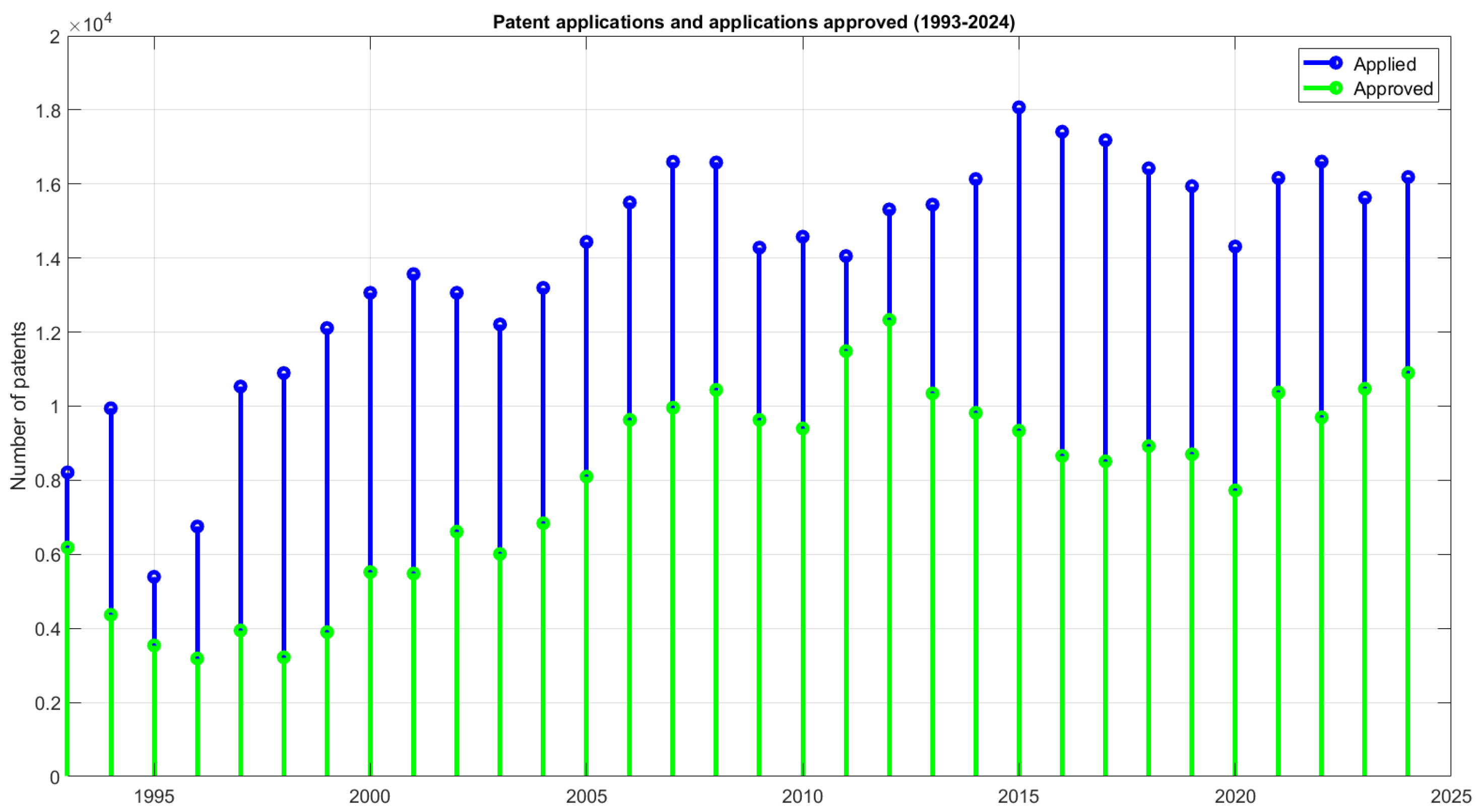
Figure 2 illustrates the behavior of patents applied with respect to applications approved in Mexico from 1993 to 2024. The analysis begins in 1993, which is when the IMPI was created.

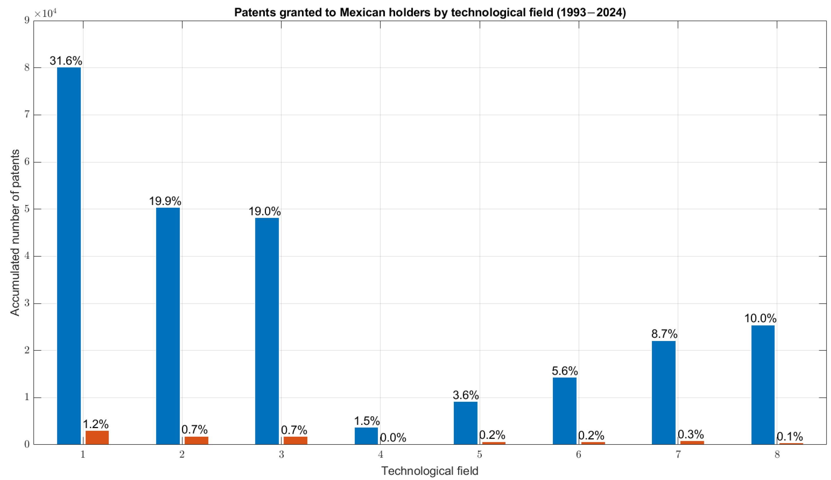
The correlation coefficient ($r=0.8$) was calculated to quantify the strength and direction of the linear relationship between the applied patents and the granted patents. On the other hand, in Mexico, IMPI uses the International Patent Classification (IPC) [47] to classify technological areas, dividing them into eight main sections. Figure 3 shows the behavior of patents granted in Mexico from 1993 to 2024, broken down by the eight different technological fields of patents and by Mexican patent holders.

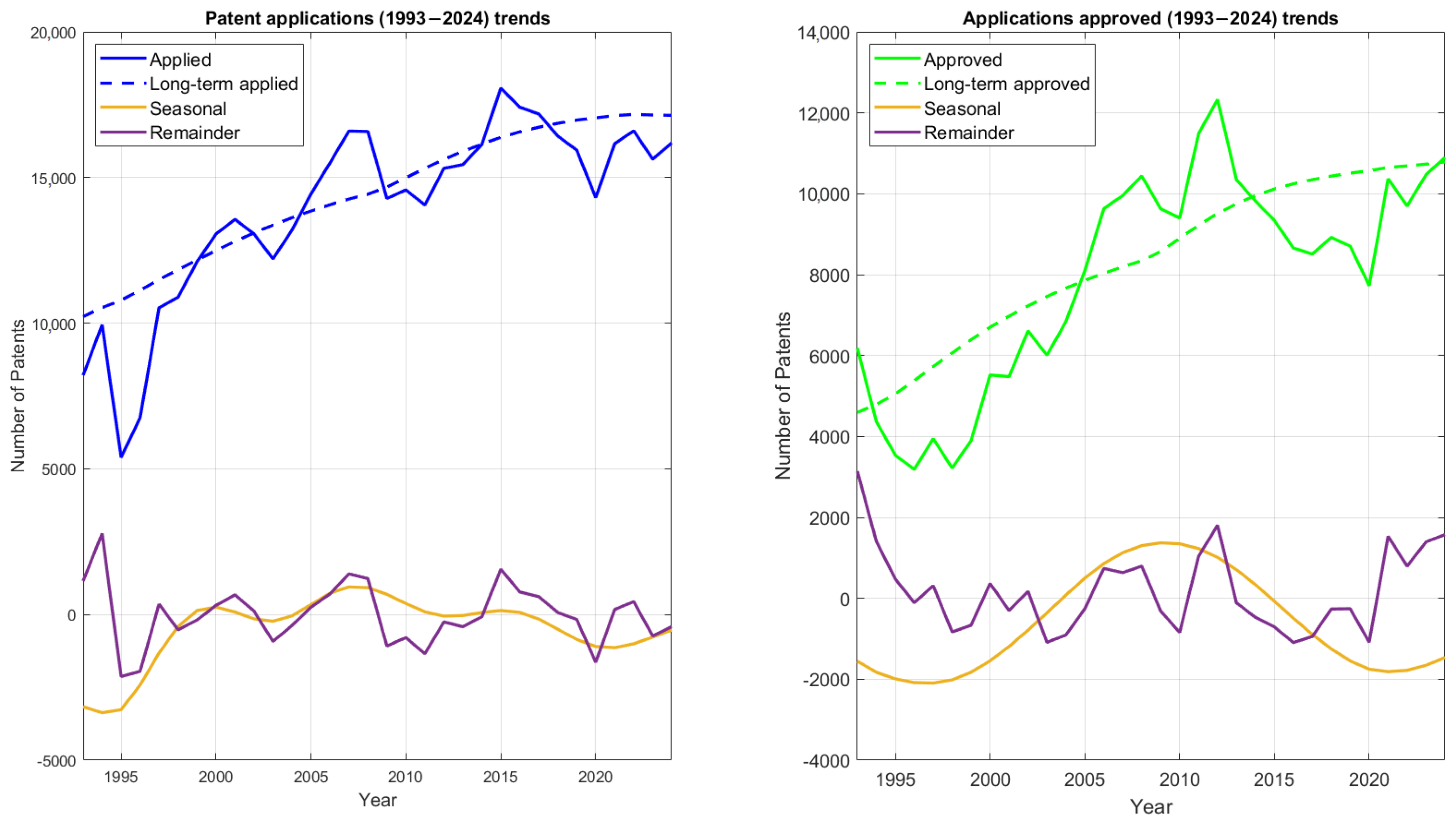
Subsequently, for exploratory data analysis, a decomposition task is performed to analyze underlying patterns and interpret the data. Regarding the normality test, the Kolmogorov–Smirnov test rejected the null hypothesis that the patent data came from a standard normal distribution. Figure 4 presents the behavior of the data from applied patents and approved applications, as well as the long-term trends, seasonality, and remaining values.

However, to measure the robustness and generalizability of each model at different points in the time series during the training stage, a rolling origin expansive technique was used. This technique was used to determine the generalization, accuracy, and variance of each model at different points in the time series, and performance metrics, including RMSE, $R^2$, and MAPE were calculated.

Table 3. RMSE, $R^2$, and MAPE results for applied patent forecasting (training dataset).

Models	RMSE				${\mathit{R}}^2$				MAPE
	Mean	Best	Median	SD	Mean	Best	Median	SD	Mean	Best	Median	SD
ARIMA	803.70	18.00	589.50	781.50	0.84	0.99	0.96	0.31	5.11	0.10	3.74	5.09
RTs	1077.60	35.88	960.42	961.31	0.58	0.99	0.90	0.80	6.60	0.25	5.70	5.66
RF	1176.15	135.83	1022.06	860.22	0.68	0.99	0.80	0.46	7.14	0.93	6.69	4.83
SVMs	894.75	1.77	664.61	746.67	0.29	0.99	0.92	1.38	5.76	0.01	4.04	5.08
LSTM	1194.30	273.85	1120.06	817.07	0.78	0.99	0.93	0.28	9.63	1.42	6.96	7.63

and

Table 4. RMSE, $R^2$, and MAPE results for granted patent forecasting (training dataset).

Models	RMSE				${\mathit{R}}^2$				MAPE
	Mean	Best	Median	SD	Mean	Best	Median	SD	Mean	Best	Median	SD
ARIMA	827.50	147.00	602.50	675.05	0.90	0.99	0.95	0.12	7.98	1.72	6.09	6.03
RTs	1065.11	97.25	996.96	900.05	0.56	0.99	0.80	0.66	10.25	1.01	11.61	7.83
RF	1366.51	67.28	1055.98	1021.76	0.18	0.99	0.75	1.51	13.32	0.65	11.83	9.01
SVMs	1033.06	2.60	719.15	956.37	0.81	0.99	0.91	0.22	9.77	0.03	7.74	8.53
LSTM	1730.93	62.02	1136.45	2351.94	0.20	0.99	0.77	1.28	28.30	0.64	11.22	56.44

summarize the performance of the five models used for the training stage: (i) ARIMA, (ii) Regression Trees, (iii) the Random Forest, (iv) Support Vector Machines, and (v) LSTM.

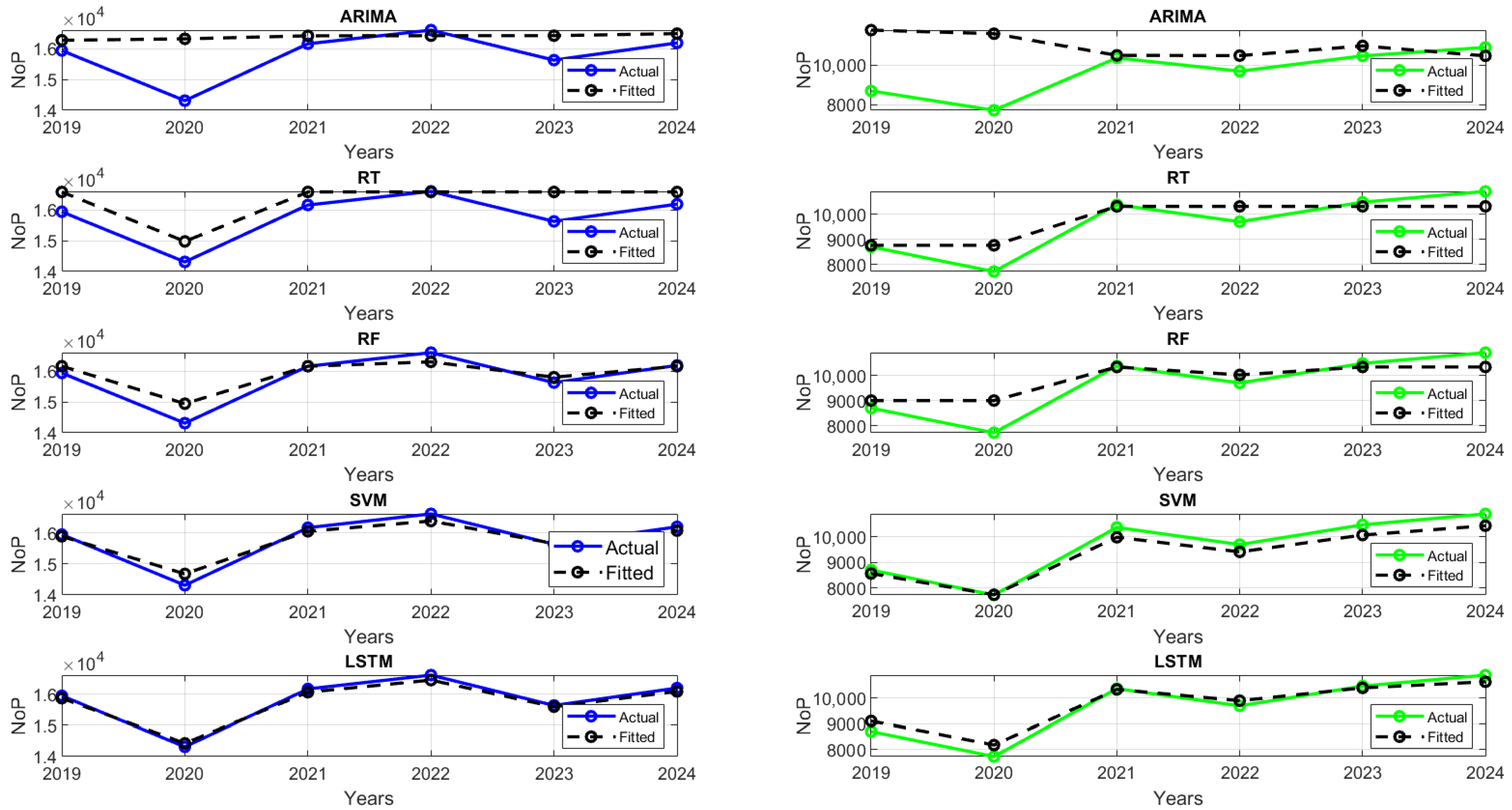
The evaluation of forecasting models is an important step in determining accuracy and reliability. Figure 5 shows the performance of the five models tested. These models have been trained with historical data and evaluated on a test dataset covering the years 2019 to 2024. The objective is to compare the predictions of each model (dashed black line) with the real values (solid blue or green line) to identify which is the most accurate.

Although this visual assessment is useful, the final selection of the best algorithm should be based on quantitative metrics such as RMSE and $R^2$.

Table 5. RMSE, $R^2$, and MAPE results for applied patent forecasting (test dataset).

Models	RMSE	${\mathit{R}}^2$	MAPE
ARIMA	910.08	−0.5	4.29
RTs	593.27	0.33	3.33
RF	308.69	0.82	1.48
SVMs	190.48	0.93	0.98
LSTM	106.91	0.97	0.63

and

Table 6. RMSE, $R^2$, and MAPE results for granted patent forecasting (test dataset).

Models	RMSE	${\mathit{R}}^2$	MAPE
ARIMA	2058.1	−1.02	17.22
RTs	552.8	0.75	4.67
RF	599.96	0.70	5.02
SVMs	322.91	0.91	2.73
LSTM	283.20	0.93	2.65

summarize the results regarding the model evaluation stage in the test dataset.

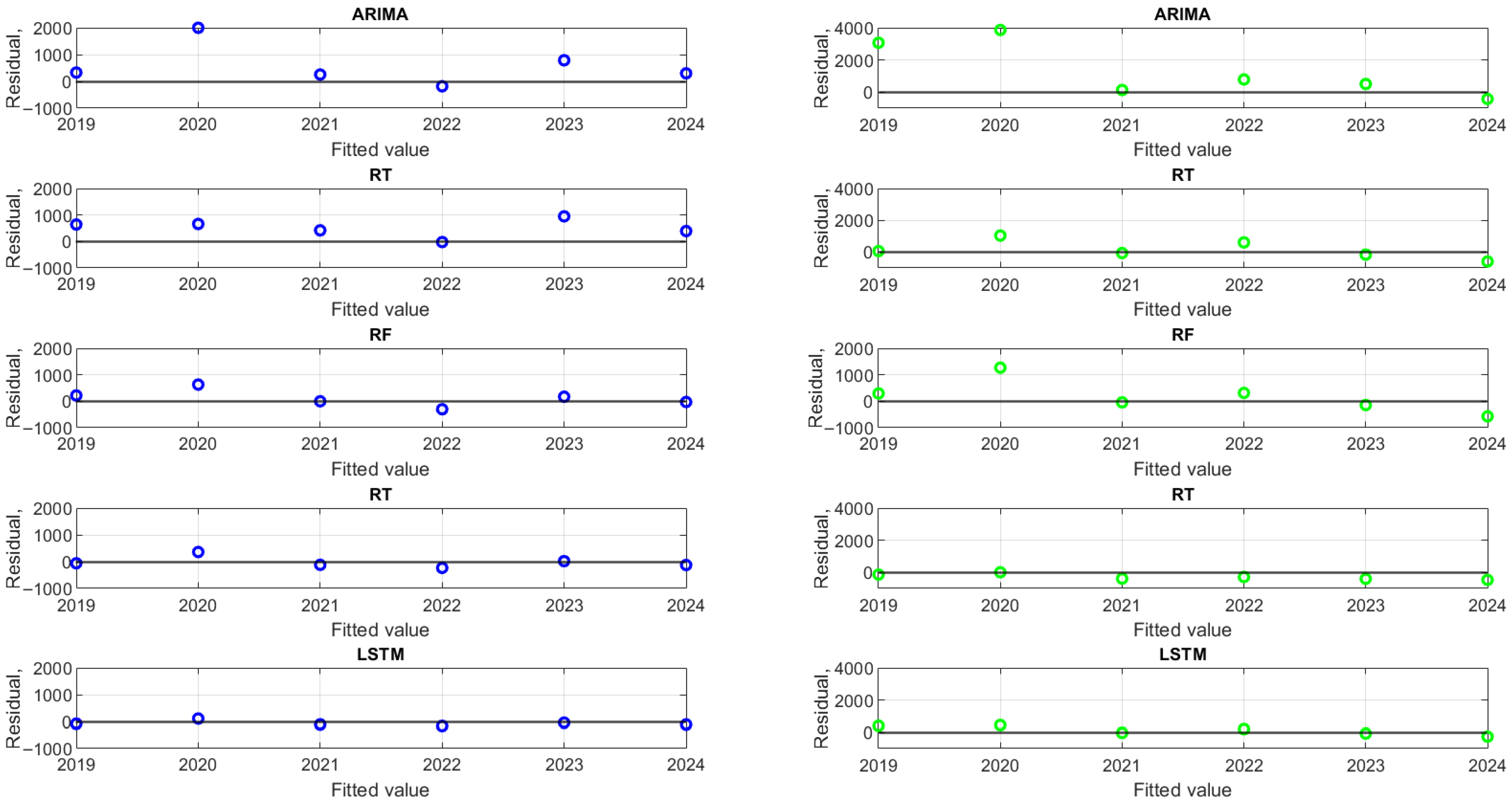
To provide methodological validation for the forecasting task, Figure 6 shows the residual plots obtained for the different models evaluated.

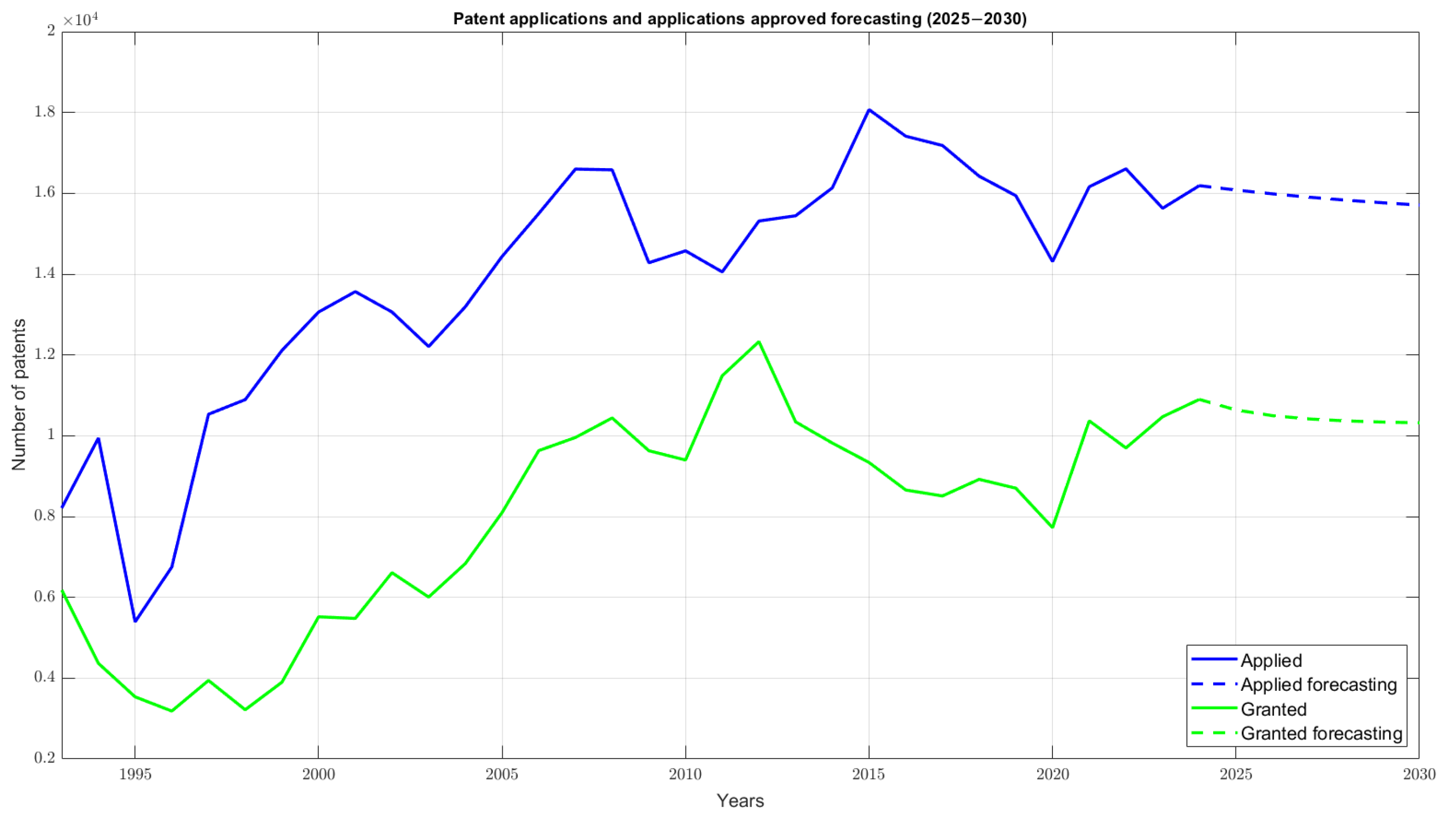
Finally, Figure 7 shows the forecast of the number of patents applied and granted in Mexico for the period 2025–2030. The solid blue line represents applied patents, while the solid green line represents granted patents. Forecasts for the future years are indicated by dashed lines of the same color. The objective of this analysis is to evaluate the historical trend and make future predictions.

4. Discussion

Initially, a Pearson correlation of $r=0.8$ indicates a strong positive linear relationship between applied and granted patent data. This could be seen as an indicator of the relative effectiveness of the national patent evaluation system, as the number of granted patents tends to increase with the number of patent applications (Figure 2). However, this behavior implies that not all patents applied for end up being granted, and this may be due to the quality of the application, the technological complexity, or even the resolution timing of the IMPI. This finding is consistent with global studies showing that stable institutional frameworks exhibit strong associations between patent applications and grants [48].

The results presented in Figure 2 show a cyclical pattern of increases and decreases in the number of patent applications and grants, reflecting the historical economic dynamics of Mexico. This pattern is consistent with observations reported for other Latin American economies [49]. The absence of a long-term industrial policy and the persistence of a maquiladora-based production model in Mexico result in limited domestic innovation. This has led to a high concentration of patents associated with transnational companies and a structural dependence on the United States and Canada [50]. However, efforts to promote industrial property through the Mexican Institute of Industrial Property (IMPI), along with an open trade policy reinforced by the North American Free Trade Agreement (NAFTA), contributed to a significant increase in patent applications and grants between 1993 and 1994, the initial years of analysis driving a productive shift toward sectors integrated with international trade.

Between 1995 and 1999, the number of patents granted was substantially reduced, a phenomenon associated with the severe economic crisis that impacted Mexico during that period. This decline directly impacted the nation’s innovation capacity and industrial performance, particularly in industries relying on the maquiladora export model, which hinders domestic innovation [9]. In response, a new institutional framework for science, technology, and innovation was established in the early 2000s with the implementation of the Law of Science and Technology in 2002 and the creation of agencies dedicated to promoting technological development and innovation. These regulatory measures contributed to a notable recovery, leading to a sustained increase in patent applications and grants between 2000 and 2012. This period is considered a boom in patent activity, reaching a historical peak in 2012 with 12,330 patents granted; this was largely driven by public policies that strengthened support for research, entrepreneurship, and the training of highly qualified human capital through postgraduate education programs.

From 2012 to 2018, Mexico maintained the institutional framework for science, technology, and innovation, promoting entrepreneurship through the National Entrepreneur Institute and supporting the training of specialized human capital. These actions strengthened inventive activity, as shown in patent applications and grants. From 2018 to 2024, patent activity remained relatively stable despite policy uncertainties in the sector. Given the average four-year delay between application and grant approval [23], a direct annual comparison is not feasible. Since the incorporation of Mexico into the General Agreement on Tariffs and Trade (GATT), the institutional and legal framework has favored the protection of industrial property [51]. However, of the 2,532,214 patents granted between 1993 and 2024, only 9090 (3.6%) were awarded to Mexican holders, revealing a persistent dependence on foreign innovation and limited technology transfer capabilities.

As shown in Figure 3, more than 70% of the patents granted in Mexico during the examined period belong to three fields: (i) consumer and utility items, (ii) miscellaneous industrial techniques and (iii) chemical and metallurgy. This concentration indicates that inventive activity during these 32 years has focused mainly on low-value domains, consistent with an export/manufacturing model, highlighting dependence on technology import. Transnational companies dominate these areas; patent holders are often nonresidents, and domestic investment in R&D has been limited. Currently, innovation output in Mexico remains limited, as technological capability is highly dependent on regional resources, institutional quality, and human capital, which are still weak in many states [52].

In the decomposition stage of the forecasting framework, time-series analysis begins by separating underlying trends, seasonal patterns, and irregular components to better characterize patent dynamics over time. According to the Kolmogorov–Smirnov normality test, the analyzed patent data do not follow a normal distribution. This has important implications for selecting appropriate forecasting models. This supports the application of non-parametric models and data decomposition methods to identify fundamental patterns, including those derived from machine learning and deep learning algorithms [15]. As shown in Figure 4, the number of patents applied and granted has increased steadily, reflecting sustained growth in recent years. With regard to seasonality, there are weak seasonal components, suggesting that patents do not present repetitive patterns marked in cycles such as months or quarters, as well as small-magnitude residuals without structured patterns, and reflecting that most of the variability is explained by the trend [53].

However, the results of cross-validation using an expanding rolling origin approach for applied patents (Table 3) and granted patents (Table 4) indicate differences in the performance of the models. In general, the ARIMA model presents the best balance between error and explanatory power, showing the lowest RMSE and MAPE values, as well as a high and stable $R^2$, demonstrating its ability to capture time-series trends without overfitting. Although tree-based models (RTs and RFs) show acceptable performance, these have higher error variability and lower consistency $R^2$, likely due to their limited representation of features. The SVM and LSTM models show more inconsistent performance; despite achieving high $R^2$ values, their higher SD and MAPE values indicate lower predictive stability, especially for LSTM, likely due to model complexity and limited training data. Overall, the results show that traditional statistical approaches, such as ARIMA, achieve performance comparable to that of machine learning models in patent time-series forecasting.

Based on visual inspection of Figure 5, for patent prediction, the LSTM model is the most reliable and accurate to predict granted patents. Meanwhile, for applied patents, the RF and LSTM offer similar performance. These results are consistent with reports in the literature on the complexity of patent prediction due to external factors and the dynamic structure of innovation ecosystems. LSTM outperforms SVMs, the RF, and RTs in predicting patent applications by effectively capturing complex temporal dynamics, as reported in recent financial and environmental forecasting studies [17,54,55].

The comparative analysis of the forecast results for applied patents (Table 5) and granted patents (Table 6), as referenced by [56], establishes that the deep learning and non-linear machine learning models outperform ARIMA. For the prediction of applied patents, the LSTM model demonstrates the best performance, achieving high accuracy, with the lowest RMSE (106.91), the highest $R^2$ (0.97), and an MAPE of only 0.63%. This dominance is maintained in the forecasting of granted patents, where LSTM obtains an RMSE of 283.20 and an $R^2$ of 0.93, with the SVM (Support Vector Machine) model achieving similar results. The ARIMA model in both series has lower performance, with negative values for $R^2$ ($-0.5$ and $-1.02$) and the highest absolute errors, indicating that the patent time series are dominated by complex non-linear dependencies and temporal structures that the linear approach fails to model. Furthermore, the increase in RMSE and MAPE values in the prediction of patents granted underscores the complexity of this task, which is attributed to the stochasticity and latency associated with the approval process.

These findings show a trade-off between model stability and predictive accuracy. The ARIMA model shows robust and consistent behavior across cross-validation folds, indicating high generalization and resistance to temporal fluctuations. In contrast, the LSTM model achieves superior predictive accuracy in the test dataset, effectively capturing the complex non-linear temporal dependencies that characterize patent dynamics. Nevertheless, this performance is accompanied by higher variability and sensitivity to training conditions, which may limit its stability in different data partitions or limited sample scenarios. Consequently, comparative analysis underscores that traditional statistical models, such as ARIMA, offer a more interpretable and stable framework for long-term trend analysis, whereas deep learning approaches such as LSTM are better suited for short-term forecasts where the capture of non-linear patterns is critical [57].

As we can see in Figure 6, for the residual plots in the test stage, the residuals are distributed around zero, indicating that there is no systematic bias in the predictions. Furthermore, the residuals do not show patterns or systematic dependence on the fitted values, which confirms that the models adequately capture the underlying relationships between the variables. A greater dispersion of residuals is observed in some models, such as ARIMA and RTs (right column), which may indicate a lower capacity to adjust extreme values or peaks in the data. However, models such as LSTM present more uniform residuals concentrated around zero, which implies a more stable and consistent fit on the test set. Taken together, these results allow us to evaluate the relative accuracy of the models and their ability to generalize on new data, with residual plots serving as a complementary tool to the analysis of quantitative metrics such as RMSE, $R^2$, and MAPE.

Finally, the analysis of patent forecasting (Figure 7) highlights several key trends. Historically, patent applications showed a positive lag, with a clear long-term upward trajectory and notable fluctuations, while granted patents have also increased over time, though not proportionally, as not all applications are accepted. For the period 2025–2030, forecasts indicate that applications will stabilize around 16,500, showing no significant growth, while granted patents are expected to decline and then remain constant at approximately 10,000. Consequently, the increasing gap between patent applications and grants offers valuable guidance for the formulation and implementation of innovation policies and the management of industrial property in the country [58].

5. Conclusions

The comparative analysis of computational forecasting models for patent applications and grants in Mexico indicates that both machine learning and deep learning approaches can accurately capture historical trends. Although the LSTM model achieved high performance in a single test period, with an RMSE of 106.91, an $R^2$ of 0.97, and an MAPE of 0.63 for applied patents and an RMSE of 283.20, an $R^2$ of 0.93, and an MAPE of 2.65 for granted patents, cross-validation revealed that the ARIMA model offers greater stability and consistency. Specifically, ARIMA obtained the lowest average RMSEs (803.70 for applied patents and 827.50 for granted patents) and the highest average $R^2$ of 0.84 for applied patents and 0.90 for granted, indicating that it provides the most reliable forecasts across multiple scenarios.

Despite the effectiveness of these models, this study has limitations. The forecasts are based on historical data and do not account for external factors such as economic fluctuations, changes in intellectual property legislation, government innovation policies, or disruptive technological advances. Additionally, the limited size of the dataset constrains the capacity of the models to learn complex patterns and generalize over the long term. Future work should focus on incorporating external indicators (e.g., GDP, R&D investment, and foreign investment) and exploring hybrid models that combine the ability of LSTM to capture sequential patterns with the stability of SVMs. Continuous evaluation in dynamic environments is recommended to maintain the accuracy and reliability of the forecast.

References

1. Beltrán-Urvina, L.I.; Acosta-Andino, B.F.; Gallegos-Varela, M.C.; Vallejos-Orbe, H.M. Intellectual Property as a Strategy for Business Development. Laws 2025, 14, 18. [Google Scholar] [CrossRef]
2. Ponta, L.; Puliga, G.; Manzini, R. A measure of innovation performance: The Innovation Patent Index. Manag. Decis. 2021, 59, 73–98. [Google Scholar] [CrossRef]
3. Gassmann, O.; Bader, M.A.; Thompson, M.J. Patent Management: Protecting Intellectual Property and Innovation; Springer: Berlin/Heidelberg, Germany, 2021. [Google Scholar]
4. Pérez Hernández, C.C.; Hernández Calzada, M.A.; Mendoza Moheno, J. Towards a knowledge economy in Mexico: Failures and Challenges. Econ. UNAM 2020, 17, 147–164. [Google Scholar]
5. Takwi, F.M. Business management and innovation: A critical analysis of small business success. Am. J. Oper. Manag. Inf. Syst. 2020, 5, 62–73. [Google Scholar] [CrossRef]
6. WIPO. Patents. Available online: https://www.wipo.int/en/web/patents/ (accessed on 2 September 2025).
7. OECD. OECD Economic Surveys: Mexico 2024. Available online: https://www.oecd.org/en/publications/oecd-economic-surveys-mexico-2024_b8d974db-en.html (accessed on 2 September 2025).
8. Díaz-Bautista, A.; González, E.D.; Andrade, S.G. Nearshoring, Comercio Internacional y Desarrollo Económico en México: Las Oportunidades de México en la Reestructuración Económica Mundial; Comunicacion Científica: Ciudad de México, Mexico, 2025. [Google Scholar]
9. Guzmán, A.; Gómez Víquez, H.; López Herrera, F. Patents and economic growth: The case of Mexico during NAFTA. Econ. Teor. y Pract. 2018, 177–213. [Google Scholar]
10. IMPI. La Contribucion Economica de la Propiedad Intelectual en Mexico. Available online: https://www.gob.mx/cms/uploads/attachment/file/663632/IP-Key-LA_Impact-Study-Mexico-2020_Report.pdf (accessed on 2 September 2025).
11. Mejía, C.; Kajikawa, Y. Patent research in academic literature: Landscape and trends with a focus on patent analytics. Front. Res. Metrics Anal. 2025, 9, 1484685. [Google Scholar] [CrossRef]
12. Ampornphan, P.; Tongngam, S. Exploring technology influencers from patent data using association rule mining and social network analysis. Information 2020, 11, 333. [Google Scholar] [CrossRef]
13. Han, S.; Huang, H.; Huang, X.; Li, Y.; Yu, R.; Zhang, J. Core patent forecasting based on graph neural networks with an application in stock markets. Technol. Anal. Strateg. Manag. 2024, 36, 1680–1694. [Google Scholar] [CrossRef]
14. Zhou, Y.; Dong, F.; Liu, Y.; Li, Z.; Du, J.; Zhang, L. Forecasting emerging technologies using data augmentation and deep learning. Scientometrics 2020, 123, 1–29. [Google Scholar] [CrossRef]
15. Yao, L.; Ni, H. Prediction of patent grant and interpreting the key determinants: An application of interpretable machine learning approach. Scientometrics 2023, 128, 4933–4969. [Google Scholar] [CrossRef]
16. Lee, C.; Kwon, O.; Kim, M.; Kwon, D. Early identification of emerging technologies: A machine learning approach using multiple patent indicators. Technol. Forecast. Soc. Change 2018, 127, 291–303. [Google Scholar] [CrossRef]
17. Jiang, H.; Fan, S.; Zhang, N.; Zhu, B. Deep learning for predicting patent application outcome: The fusion of text and network embeddings. J. Inf. 2023, 17, 101402. [Google Scholar] [CrossRef]
18. Zhang, Y.; Wang, Q. Patent prediction based on long short-term memory recurrent neural network. In Proceedings of the 9th International Conference on Computer Engineering and Networks, Changsha, China, 18–20 October 2021; Springer: Singapore, 2021; pp. 291–299. [Google Scholar]
19. Tsai, M.C. A homogenous forecast model based on the hybrid imputation method for forecasting national patent application numbers. Multimed. Tools Appl. 2024, 83, 41137–41169. [Google Scholar] [CrossRef]
20. Wang, J.; Wang, L.; Ji, N.; Ding, Q.; Zhang, F.; Long, Y.; Ye, X.; Chen, Y. Enhancing patent text classification with Bi-LSTM technique and alpine skiing optimization for improved diagnostic accuracy. Multimed. Tools Appl. 2025, 84, 9257–9286. [Google Scholar] [CrossRef]
21. Miller, J.A.; Aldosari, M.; Saeed, F.; Barna, N.H.; Rana, S.; Arpinar, I.B.; Liu, N. A survey of deep learning and foundation models for time series forecasting. arXiv 2024, arXiv:2401.13912. [Google Scholar] [CrossRef]
22. Maragakis, M.; Rouni, M.A.; Mouza, E.; Kanetidis, M.; Argyrakis, P. Tracing technological shifts: Time-series analysis of correlations between patent classes. Eur. Phys. J. Plus 2023, 138, 776. [Google Scholar] [CrossRef]
23. Instituto Mexicano de la Propiedad Industrial (IMPI). IMPI in Numbers. Available online: https://docs.google.com/spreadsheets/d/11DJblFCsGsH_PxKFambn3uxF289r7l3w/edit?gid=1930750129#gid=1930750129 (accessed on 2 September 2025).
24. Soto-Rubio, M.; Germán-Soto, V.; Gutiérrez Flores, L. Patentes, tamaño de empresa y financiamiento público en México: Análisis regional con modelos de datos de conteo. Rev. Mex. Econ. Finanz. 2023, 18, e569. [Google Scholar] [CrossRef]
25. Meisenbacher, S.; Turowski, M.; Phipps, K.; Rätz, M.; Müller, D.; Hagenmeyer, V.; Mikut, R. Review of automated time series forecasting pipelines. Wiley Interdiscip. Rev. Data Min. Knowl. Discov. 2022, 12, e1475. [Google Scholar] [CrossRef]
26. Zhang, X.; Li, R. A novel decomposition and combination technique for forecasting monthly electricity consumption. Front. Energy Res. 2021, 9, 792358. [Google Scholar] [CrossRef]
27. Golyandina, N.; Korobeynikov, A.; Zhigljavsky, A. Singular Spectrum Analysis with R; Springer: Berlin/Heidelberg, Germany, 2018; p. 83. [Google Scholar]
28. Matamoros, A.A.; Nieto-Reyes, A.; Agostinelli, C. nortsTest: An R Package for Assessing Normality of Stationary Processes. R J. 2025, 16, 135–156. [Google Scholar] [CrossRef]
29. Kwon, K.; Jun, S.; Lee, Y.J.; Choi, S.; Lee, C. Logistics technology forecasting framework using patent analysis for technology roadmap. Sustainability 2022, 14, 5430. [Google Scholar] [CrossRef]
30. Kim, J.; Kim, H.; Kim, H.; Lee, D.; Yoon, S. A comprehensive survey of deep learning for time series forecasting: Architectural diversity and open challenges. Artif. Intell. Rev. 2025, 58, 1–95. [Google Scholar] [CrossRef]
31. Park, M.J.; Yang, H.S. Comparative study of time series analysis algorithms suitable for short-term forecasting in implementing demand response based on AMI. Sensors 2024, 24, 7205. [Google Scholar] [CrossRef]
32. Fathi, S.; Srinivasan, R.; Fenner, A.; Fathi, S. Machine learning applications in urban building energy performance forecasting: A systematic review. Renew. Sustain. Energy Rev. 2020, 133, 110287. [Google Scholar] [CrossRef]
33. Masini, R.P.; Medeiros, M.C.; Mendes, E.F. Machine learning advances for time series forecasting. J. Econ. Surv. 2023, 37, 76–111. [Google Scholar] [CrossRef]
34. Lin, T.Y.; Chou, L.C. A systematic review of artificial intelligence applications and methodological advances in patent analysis. World Pat. Inf. 2025, 82, 102383. [Google Scholar] [CrossRef]
35. Wang, M.; Pan, J.; Li, X.; Li, M.; Liu, Z.; Zhao, Q.; Luo, L.; Chen, H.; Chen, S.; Jiang, F.; et al. ARIMA and ARIMA-ERNN models for prediction of pertussis incidence in mainland China from 2004 to 2021. BMC Public Health 2022, 22, 1447. [Google Scholar] [CrossRef]
36. Erciyes, K. Algebraic Graph Algorithms; Springer International Publishing: Cham, Switzerland, 2021. [Google Scholar]
37. Hu, J.; Szymczak, S. A review on longitudinal data analysis with random forest. Briefings Bioinform. 2023, 24, bbad002. [Google Scholar] [CrossRef] [PubMed]
38. Eom, H.; Choi, S.; Choi, S.O. Marketable value estimation of patents using ensemble learning methodology: Focusing on US patents for the electricity sector. PLoS ONE 2021, 16, e0257086. [Google Scholar] [CrossRef] [PubMed]
39. Wang, M.H.; Che, H.C. Intellectual capital forecasting for invention patent through machine learning model. J. Intellect. Cap. 2024, 25, 129–150. [Google Scholar] [CrossRef]
40. Han, J.; Pei, J.; Tong, H. Data Mining: Concepts and Techniques; Morgan Kaufmann: Burlington, MA, USA, 2022. [Google Scholar]
41. She, Y.; Hong, Y.; Shen, S.; Yang, B.; Zhang, L.; Wang, J. Consistency regularization for few shot multivariate time series forecasting. Sci. Rep. 2025, 15, 14195. [Google Scholar] [CrossRef] [PubMed]
42. Chicco, D.; Warrens, M.J.; Jurman, G. The coefficient of determination R-squared is more informative than SMAPE, MAE, MAPE, MSE and RMSE in regression analysis evaluation. PeerJ Comput. Sci. 2021, 7, e623. [Google Scholar] [CrossRef]
43. Athiyarath, S.; Paul, M.; Krishnaswamy, S. A comparative study and analysis of time series forecasting techniques. SN Comput. Sci. 2020, 1, 175. [Google Scholar] [CrossRef]
44. Makridakis, S.; Spiliotis, E.; Assimakopoulos, V. M5 accuracy competition: Results, findings, and conclusions. Int. J. Forecast. 2022, 38, 1346–1364. [Google Scholar] [CrossRef]
45. Yang, L.; Shami, A. On hyperparameter optimization of machine learning algorithms: Theory and practice. Neurocomputing 2020, 415, 295–316. [Google Scholar] [CrossRef]
46. Shahriari, B.; Swersky, K.; Wang, Z.; Adams, R.P.; De Freitas, N. Taking the human out of the loop: A review of Bayesian optimization. Proc. IEEE 2015, 104, 148–175. [Google Scholar] [CrossRef]
47. Sasaki, H.; Sakata, I. Identifying potential technological spin-offs using hierarchical information in international patent classification. Technovation 2021, 100, 102192. [Google Scholar] [CrossRef]
48. Gürler, M. The effect of the researchers, research and development expenditure as innovation inputs on patent grants and high-tech exports as innovation outputs in OECD and emerging countries especially in BRIICS. Avrupa Bilim Teknol. Derg. 2021, 32, 1140–1149. [Google Scholar] [CrossRef]
49. Romero-Betancur, J.D. Colombian technological panorama: An approach from pa-tent applications in Colombia between 2000 and 2018. Rev. Cient. 2021, 40, 89–101. [Google Scholar] [CrossRef]
50. Olvera, S.G. Paradojas de la innovación y la migración calificada de inventores en el contexto neoliberal: Reflexiones en torno al caso mexicano. Migr. y Desarro. 2021, 19, 143–175. [Google Scholar] [CrossRef]
51. Mondragón, J.J.P. Propiedad intelectual y comercio internacional. Rev. Fac. Derecho Mex. 2019, 69, 855–878. [Google Scholar] [CrossRef]
52. Pérez Hernández, C.C. Determinantes de la capacidad tecnológica en México: Factores meso económicos que impulsan los productos tecno-científicos. Contad. y Adm. 2020, 65, e158. [Google Scholar]
53. Zou, T.; Yu, L.; Sun, L.; Du, B.; Wang, D.; Zhuang, F. Event-based dynamic graph representation learning for patent application Trend Prediction. IEEE Trans. Knowl. Data Eng. 2023, 36, 1951–1963. [Google Scholar] [CrossRef]
54. Dehghani, A.; Moazam, H.M.Z.H.; Mortazavizadeh, F.; Ranjbar, V.; Mirzaei, M.; Mortezavi, S.; Ng, J.L.; Dehghani, A. Comparative evaluation of LSTM, CNN, and ConvLSTM for hourly short-term streamflow forecasting using deep learning approaches. Ecol. Inform. 2023, 75, 102119. [Google Scholar] [CrossRef]
55. Shobayo, O.; Adeyemi-Longe, S.; Popoola, O.; Okoyeigbo, O. A Comparative Analysis of Machine Learning and Deep Learning Techniques for Accurate Market Price Forecasting. Analytics 2025, 4, 5. [Google Scholar] [CrossRef]
56. Kamateri, E.; Stamatis, V.; Diamantaras, K.; Salampasis, M. Automated single-label patent classification using ensemble classifiers [Conference paper]. In Proceedings of the 2022 14th International Conference on Machine Learning and Computing, Suzhou, China, 18–21 February 2022; pp. 324–330. [Google Scholar]
57. Lahboub, K.; Benali, M. Assessing the predictive power of transformers, ARIMA, and LSTM in forecasting stock prices of Moroccan credit companies. J. Risk Financ. Manag. 2024, 17, 293. [Google Scholar] [CrossRef]
58. Castillo-Esparza, M.M.G.C.; Cuevas-Pichardo, L.J.; Montejano-García, S. Innovation in Mexico: Patents, R&D expenditure and human capital. Sci. Prax. 2022, 2, 82–103. [Google Scholar]
Figure 1. Workflow for analyzing time-series patent data.
Inventions 10 00102 g001
Figure 2. Patent applications, applications approved (1993–2024), and trends for long-term analysis [23].
Inventions 10 00102 g002
Figure 3. Patent granted by technological field (1993–2024) [23].
Inventions 10 00102 g003
Figure 4. Annual trends in applied and approved application patents (1993–2024).
Inventions 10 00102 g004
Figure 5. Predicted and actual trends of patent applications (left) and granted patents (right) for the test set (2019–2024).
Inventions 10 00102 g005
Figure 6. Residual plots of the models evaluated in the testing stage.
Inventions 10 00102 g006
Figure 7. Patent applications and applications approved (2025–2030) based on long-term forecasting.
Inventions 10 00102 g007