Mathematical Modeling of the Influence of Electrical Heterogeneity on the Processes of Salt Ion Transfer in Membrane Systems with Axial Symmetry Taking into Account Electroconvection

Abstract

This article proposes a 3D mathematical model of the influence of electrical heterogeneity of the ion exchange membrane surface on the processes of salt ion transfer in membrane systems with axial symmetry; in particular, we investigate an annular membrane disk in the form of a coupled system of Nernst–Planck–Poisson and Navier–Stokes equations in a cylindrical coordinate system. A hybrid numerical–analytical method for solving the boundary value problem is proposed, and a comparison of the results for the annular disk model obtained by the hybrid method and the independent finite element method is carried out. The areas of applicability of each of these methods are determined. The proposed model of an annular disk takes into account electroconvection, which is understood as the movement of an electrolyte solution under the action of an external electric field on an extended region of space charge formed at the solution–membrane boundary under the action of the same electric field. The main regularities and features of the occurrence and development of electroconvection associated with the electrical heterogeneity of the surface of the membrane disk of the annular membrane disk are determined; namely, it is shown that electroconvective vortices arise at the junction of the conductivity and non-conductivity regions at a certain ratio of the potential jump and angular velocity and flow down in the radial direction to the edge of the annular membrane. At a fixed potential jump greater than the limiting one, the formed electroconvective vortices gradually decrease with an increase in the angular velocity of rotation until they disappear. Conversely, at a fixed value of the angular velocity of rotation, electroconvective vortices arise at a certain potential jump, and with its subsequent increase gradually increase in size.

1. Introduction

The operation of electromembrane systems (EMS) in overlimit current modes has significant potential for a significant reduction in investment costs for desalination plants. The study by Wessling et al. [1] was devoted to the analysis of electroconvective vortices using the surface patterning method or geometric and electrical heterogeneity. In [1], a comparison of electroconvection development on two membranes modified using patterns was performed. An analysis was carried out of the increase in area of the electroconvective vortices, their structural stability in a steady state, and the possibility of controlling electroconvective vortices by introducing certain structural heterogeneities of the membrane surface to reduce energy losses in the current–voltage characteristic (CVC) and for more economical operation in EMS in overlimit modes, significantly increasing their efficiency.

As [2,3,4,5,6,7] show, the phenomenon of overlimit mass transfer is currently being intensively studied; however, many issues are still poorly understood. For example, it is necessary to study the effects modifications of the membrane surface have on the development of electroconvection. Electrical inhomogeneity arises due to the inhomogeneous distribution of charges on the membrane surface, which can be caused by both the geometric features of the system [8,9] and the properties of the membrane material. Such inhomogeneities lead to local zones with increased electric field strength, which in turn affects the rate of ion migration and accordingly the emergence and development of electroconvective vortices. In turn, this leads to an increase in the rate of ion transfer through the membrane.

In [10], it was shown that the electrical conductivity from an electrolyte solution to a solid element with a selective charge, such as an ion exchange membrane or an electrode, becomes unstable when the electrolyte concentration near the interface approaches zero due to diffusion limitation. In [11], an analysis was made of the influence of the fine structure of the electrical double layer and the reaction rate of the electrode on the choice of the wavelength of the increasing perturbation mode with morphological instability during cathodic electrodeposition from a dilute electrolyte solution.

In recent years, there has been significant progress in understanding the role of electrical heterogeneity and electroconvection in EMS. Thus, a previous study [12] was devoted to the mechanism of development of electroconvective vortices, and their development was also controlled using a one-dimensional ion exchange membrane with a mesh pattern (IEM). It was shown that the rate of decrease in the electric potential rapidly increased during the development of vortices but gradually decreased during the transverse merging of vortices. Based on these data on the electroconvective vortex, it was shown that the electrical inhomogeneity of the IEM actively controls the vortex and increases the desalination efficiency.

A new model was proposed in [13] that takes into account non-linear effects in electroconvection, which allowed for a more accurate description of mass transfer processes under high current density conditions.

In [14], non-stationary ion transport caused by a sinusoidal current through an ion exchange membrane with an electrically inhomogeneous surface was considered. Low-frequency spectra of the electrochemical impedance of electrically inhomogeneous ion exchange membranes were studied experimentally and theoretically, and a two-dimensional model for calculating these spectra was proposed. Non-stationary ion transport through a heterogeneous membrane and two adjacent diffusion layers was studied. Numerical and analytical (under conditions of equality of the diffusion coefficients of the cation and anion in the solution and at zero direct bias current) solutions were obtained for the corresponding two-dimensional boundary value problem.

In [15], the study focused on experiments with heterogeneous membranes MK-40 and MA-41 with different ion exchange resin contents. It was found that the electrical conductivity of both cation exchange and anion exchange membranes increased with the increasing ion exchange resin content, with cation exchange membranes demonstrating a wider range of change.

Thus, the study of electrical heterogeneity and its effect on ion transport with electroconvection taken into account is an important area of research into increasing the efficiency of the separation and purification of solutions, and is of great practical importance. Further theoretical research in this area should be aimed at developing more accurate mathematical models. The advantage of constructing 3D models with axial symmetry is the property of equal accessibility at sub = limiting currents, i.e., the fact that the thickness of the diffusion layer in such systems is constant up until the moment of the onset of electroconvection. At the same time, we note the insufficient development of such mathematical models and numerical methods for solving boundary value problems for overlimit current modes.

This article is a continuation of [16], where the basic 3D model of electroconvection with axial symmetry was formulated and investigated. In this article, a modification of the basic model is considered, which consists of considering a cation exchange membrane of a more general type with conductivity and non-conductivity sections. As a result, an annular cation exchange membrane disk is obtained, new boundary conditions are formulated for non-conductivity sections, and their coordination with the conductivity sections on the cation exchange membrane is achieved. Thus, a mathematical model of a much more general type is obtained, which accordingly is more adequate and applicable for the study of heterogeneous cation exchange membranes used in practice than that considered in [16].

2. Methods

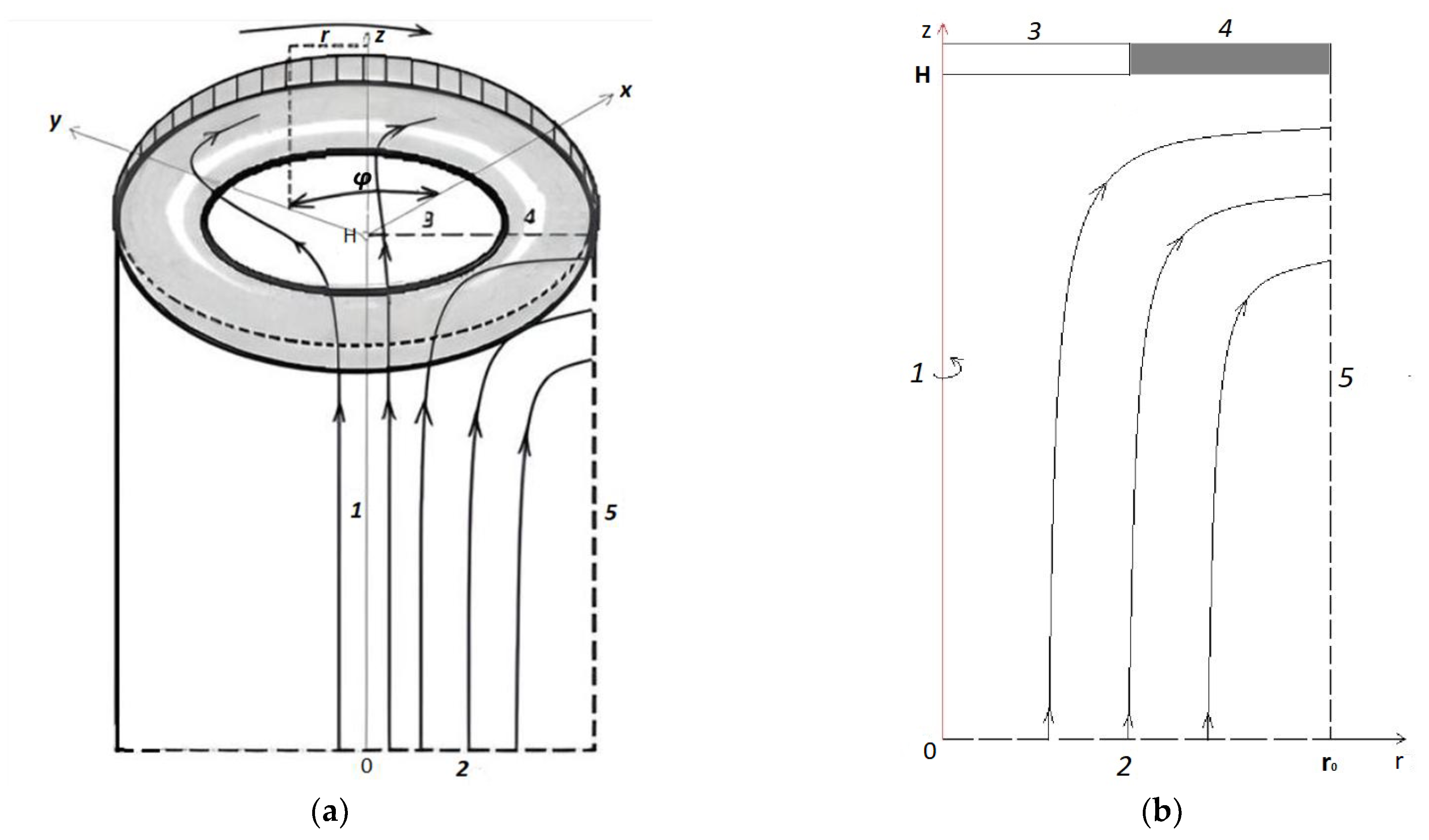
2.1. Mathematical Model of Transport for Annular Membrane Disk

Let us consider the transfer of salt ions during rotation of a cation exchange membrane disk, with non-conducting and conducting regions, inside a vertically standing cylindrical cell around the central axis, taking into account electroconvection, after which we will formulate the corresponding mathematical model.

When formulating a mathematical model, as well as the subsequent numerical solution due to axial symmetry (Figure 1a), it is sufficient to describe half of the cross-section of the cylindrical region, where it is necessary to determine the equations and boundary conditions (Figure 1b). To do this, it is necessary to move from a rectangular coordinate system $(x,y,z)$ to a cylindrical one $(r,\phi ,z)$. However, the velocities in the angular direction differ from zero, so the model must include all three components of velocity (radial, azimuthal and axial), the flows, and the electric field strength, although they depend only on two arguments $(r,z)$, i.e., a 2D model. Moreover, with axial symmetry, the derivatives with respect to the component $\phi$ are zero, so all equations in the cylindrical coordinate system can be simplified in this case.

To model the transfer processes, a coupled system of Navier–Stokes equations with volumetric electric force $\overrightarrow{f}$ and Nernst–Planck–Poisson equations was used, which in a cylindrical coordinate system $(r,\phi ,z)$ takes the following form [16]:

$$\rho {\displaystyle \frac{\partial u}{\partial t}}+\rho \left(u{\displaystyle \frac{\partial u}{\partial r}}-{\displaystyle \frac{v^2}{r}}+w{\displaystyle \frac{\partial u}{\partial z}}\right)+{\displaystyle \frac{\partial p}{\partial r}}=\eta \left[{\displaystyle \frac{1}{r}}{\displaystyle \frac{\partial }{\partial r}}\left(r{\displaystyle \frac{\partial u}{\partial r}}\right)-{\displaystyle \frac{u}{r^2}}+{\displaystyle \frac{{\partial }^{2}u}{\partial z^2}}\right]+f_r$$

$$\rho {\displaystyle \frac{\partial v}{\partial t}}+\rho \left(u{\displaystyle \frac{\partial v}{\partial r}}-{\displaystyle \frac{uv}{r}}+w{\displaystyle \frac{\partial v}{\partial z}}\right)=\eta \left[{\displaystyle \frac{1}{r}}{\displaystyle \frac{\partial }{\partial r}}\left(r{\displaystyle \frac{\partial v}{\partial r}}\right)-{\displaystyle \frac{v}{r^2}}+{\displaystyle \frac{{\partial }^{2}v}{\partial z^2}}\right]+f_{\phi }$$

$$\rho {\displaystyle \frac{\partial w}{\partial t}}+\rho \left(u{\displaystyle \frac{\partial w}{\partial r}}+w{\displaystyle \frac{\partial w}{\partial z}}\right)+{\displaystyle \frac{\partial p}{\partial z}}=\eta \left[{\displaystyle \frac{1}{r}}{\displaystyle \frac{\partial }{\partial r}}\left(r{\displaystyle \frac{\partial w}{\partial r}}\right)+{\displaystyle \frac{{\partial }^{2}w}{\partial z^2}}\right]+f_z$$

$${\overrightarrow{j}}_i=({\displaystyle \frac{F}{RT}}{z}_i{D}_i{C}_i{E}_r-D_i{\displaystyle \frac{\partial C_i}{\partial r}}+C_{i}u){\overrightarrow{e}}_r+C_{i}v{\overrightarrow{e}}_{\phi }+({\displaystyle \frac{F}{RT}}{z}_i{D}_i{C}_i{E}_z-D_i{\displaystyle \frac{\partial C_i}{\partial z}}+C_{i}w){\overrightarrow{e}}_z$$

(1)

$${\displaystyle \frac{\partial C_i}{\partial t}}=-{\displaystyle \frac{1}{r}}{\displaystyle \frac{\partial }{\partial r}}(r{j}_{i,r})-{\displaystyle \frac{\partial j_{i,z}}{\partial z}},\hspace{0.17em}\hspace{0.17em}\hspace{0.17em}\hspace{0.17em}i=1,2\hspace{0.17em}\hspace{0.17em}\hspace{0.17em}\hspace{0.17em}$$

(2)

$${\displaystyle \frac{{\partial }^2\mathsf{\Phi }}{\partial r^2}}+{\displaystyle \frac{{\partial }^2\mathsf{\Phi }}{\partial z^2}}=-{\displaystyle \frac{1}{r}}{\displaystyle \frac{\partial \mathsf{\Phi }}{\partial r}}-{\displaystyle \frac{F}{\epsilon }}(z_1{C}_1+z_2{C}_2)$$

(3)

$$\overrightarrow{I}=F(z_1{\overrightarrow{j}}_1+z_2{\overrightarrow{j}}_2)$$

(4)

where

$$f_r=\epsilon \left({\displaystyle \frac{{\partial }^2\mathsf{\Phi }}{\partial r^2}}+{\displaystyle \frac{{\partial }^2\mathsf{\Phi }}{\partial z^2}}\right){\displaystyle \frac{\partial \mathsf{\Phi }}{\partial r}}+{\displaystyle \frac{\epsilon }{r}}{\left({\displaystyle \frac{\partial \mathsf{\Phi }}{\partial r}}\right)}^2$$

$$f_{\phi }=0$$

$$f_z=\epsilon \left({\displaystyle \frac{{\partial }^2\mathsf{\Phi }}{\partial r^2}}+{\displaystyle \frac{{\partial }^2\mathsf{\Phi }}{\partial z^2}}\right){\displaystyle \frac{\partial \mathsf{\Phi }}{\partial z}}+{\displaystyle \frac{\epsilon }{r}}{\displaystyle \frac{\partial \mathsf{\Phi }}{\partial r}}{\displaystyle \frac{\partial \mathsf{\Phi }}{\partial z}}$$

Here, $\overrightarrow{u}=(u,v,w)$; $u,v,w$—radial, azimuthal, and axial components of the solution flow velocity $\overrightarrow{u}$; index 1 refers to cations, index 2 to anions; ${\overrightarrow{j}}_1,{\overrightarrow{j}}_2$—flows; $C_1,C_2$—concentration in the solution; $z_1,z_2$—charge numbers; $\overrightarrow{I}$—current density; $D_1,\hspace{0.33em}{D}_2$—diffusion coefficients; $\mathsf{\Phi }$—electric field potential; $\overrightarrow{E}=-\nabla \mathsf{\Phi }$—electric field strength; $\epsilon$—dielectric permeability of the electrolyte; $F$—Faraday constant; $R$—universal gas constant; $T$—absolute temperature; $t$—time; $\rho$—density; $\eta$—dynamic viscosity; $p$—pressure.

In the studied section of the cylindrical region (Figure 1), boundary 2 models the part of space infinitely distant from the CEM, in which the condition of electroneutrality is satisfied and the concentration of the solution is constant ($C_0$). Boundary 2 is also considered an anode and an open boundary (inlet) for the solution; for the velocity here the condition of the absence of normal voltage is set, and the pressure is considered equal to zero. This boundary is considered an equipotential surface, and $\mathsf{\Phi }(t,r,0)=d_{\phi }$. Boundary 1 is the axis of symmetry. Boundary 5 is considered the outlet for the solution; therefore, the condition of removal of ions only by convective flow is set as ${\overrightarrow{j}}_i=-\overrightarrow{u}\cdot C_i,\hspace{0.17em}i=1,2$, and for the velocity the condition is the absence of normal stress. In addition, for the potential, the boundary condition is used, $-\overrightarrow{n}\cdot {(r{\displaystyle \frac{\partial \mathsf{\Phi }}{\partial r}},{\displaystyle \frac{\partial \mathsf{\Phi }}{\partial z}})}^T=0$; here, $\overrightarrow{n}$ is the normal vector. At boundary 4, the CEM surface is considered equipotential: $\mathsf{\Phi }(t,r,H)=d_0=0$. Boundaries 3 and 4 correspond to the rotating CEM, while for the azimuthal velocity the condition is $v(t,r,H)=\omega r$, where $\omega$ is the angular velocity of rotation of the disk. For anions, the condition of impermeability (absence of flow) is set here as $-\overrightarrow{n}\cdot {\overrightarrow{j}}_2=0$. The conductivity region is located at boundary 4, so the cation exchange membrane forms a ring (Figure 1b). At boundary 3, corresponding to the non-conducting region, there is a condition of impermeability (no flow) of $-\overrightarrow{n}\cdot {\overrightarrow{j}}_i=0$, $\hspace{0.17em}i=1,2$. To derive the condition for the potential at the non-conducting boundary 3, the equality of the current density $\overrightarrow{I}$ to zero at this boundary is used. The normal component of the current density at this boundary is equal to zero due to the conditions on the flows. We determine the radial component of the potential gradient from the condition that the radial component of the current density ass equal to zero from the formula for the current (4):

$$\begin{array}{l}\overrightarrow{I}=F(-{\displaystyle \frac{F}{RT}}(z_1^2{D}_1{C}_1+z_2^2{D}_2{C}_2){\displaystyle \frac{\partial \mathsf{\Phi }}{\partial r}}-(z_1{D}_1{\displaystyle \frac{\partial C_1}{\partial r}}+z_2{D}_2{\displaystyle \frac{\partial C_2}{\partial r}})+(z_1{C}_1+z_2{C}_2)u){\overrightarrow{e}}_r+\\ +((z_1{C}_1+z_2{C}_2)v){\overrightarrow{e}}_{\phi }+\\ +F(-{\displaystyle \frac{F}{RT}}(z_1^2{D}_1{C}_1+z_2^2{D}_2{C}_2){\displaystyle \frac{\partial \mathsf{\Phi }}{\partial z}}-(z_1{D}_1{\displaystyle \frac{\partial C_1}{\partial z}}+z_2{D}_2{\displaystyle \frac{\partial C_2}{\partial z}})+(z_1{C}_1+z_2{C}_2)w){\overrightarrow{e}}_z\end{array}$$

Therefore, from $I_r=0$, we get:

$$F(-{\displaystyle \frac{F}{RT}}(z_1^2{D}_1{C}_1+z_2^2{D}_2{C}_2){\displaystyle \frac{\partial \mathsf{\Phi }}{\partial r}}-(z_1{D}_1{\displaystyle \frac{\partial C_1}{\partial r}}+z_2{D}_2{\displaystyle \frac{\partial C_2}{\partial r}})+(z_1{C}_1+z_2{C}_2)u)=0$$

Since the radial component of the velocity is $u=0$, we obtain:

$$-{\displaystyle \frac{F}{RT}}(z_1^2{D}_1{C}_1+z_2^2{D}_2{C}_2){\displaystyle \frac{\partial \mathsf{\Phi }}{\partial r}}-(z_1{D}_1{\displaystyle \frac{\partial C_1}{\partial r}}+z_2{D}_2{\displaystyle \frac{\partial C_2}{\partial r}})=0$$

From here: ${\displaystyle \frac{\partial \mathsf{\Phi }}{\partial r}}=-{\displaystyle \frac{RT(z_1{D}_1\frac{\partial C_1}{\partial r}+z_2{D}_2\frac{\partial C_2}{\partial r})}{F(z_1^2{D}_1{C}_1+z_2^2{D}_2{C}_2)}}$.

Thus, at boundary 3, the following condition must be set for the potential:

$${\displaystyle \frac{\partial \mathsf{\Phi }}{\partial r}}=-{\displaystyle \frac{RT(z_1{D}_1\frac{\partial C_1}{\partial r}+z_2{D}_2\frac{\partial C_2}{\partial r})}{F(z_1^2{D}_1{C}_1+z_2^2{D}_2{C}_2)}}$$

It is assumed that the cell is initially completely filled with an ideally mixed solution of sodium chloride with a concentration $C_0$, and the same ideally mixed solution is fed into it through the boundary 2. Therefore, a constant concentration is taken as the initial condition $C_1(0,r,z)=C_2(0,r,z)=C_0$.

2.2. Algorithm for Hybrid Numerical–Analytical Solution

In order to clarify the problems of the numerical solution of the boundary value problem, we will move to a dimensionless form using characteristic quantities.

The problem has two characteristic quantities, where $H$ is the cell height and $r_0$ is the outer radius of the annular membrane. Since in practice $H=a\cdot r_0$, where proportionality coefficient $a=1÷5$, they have the same order, and $r_0$ is taken as a characteristic quantity, since it is convenient to express the characteristic speed through it. As the characteristic velocity $V_0$, we will use the azimuthal component of the velocity $V_0={\omega }_0{r}_0$.

Let us assume that:

$$\begin{gathered} r^{(u)}={\displaystyle \frac{r}{r_0}};\hspace{0.17em}\hspace{0.17em}\hspace{0.17em}\hspace{0.17em}{z}^{(u)}={\displaystyle \frac{z}{r_0}};\hspace{0.17em}\hspace{0.17em}\hspace{0.17em}\hspace{0.17em}{t}^{(u)}={\displaystyle \frac{t{V}_0}{r_0}};\hspace{0.17em}{\overrightarrow{u}}^{(u)}={\displaystyle \frac{\overrightarrow{u}}{V_0}};\hspace{0.17em}{C}_i^{(u)}={\displaystyle \frac{C_i}{C_0}}; {\overrightarrow{j}}_i^{(u)}={\displaystyle \frac{{\overrightarrow{j}}_i}{j_0}}; \\ {\displaystyle \frac{D_0{C}_0}{r_0}}{\overrightarrow{j}}_i^{(u)}={\overrightarrow{j}}_i; \end{gathered}$$

$$D_i^{(u)}={\displaystyle \frac{D_i}{D_0}};{\overrightarrow{E}}^{(u)}={\displaystyle \frac{r_{0}F}{RT}}\overrightarrow{E}; Pe={\displaystyle \frac{r_0{V}_0}{D_0}}; {\epsilon }^{(u)}={\displaystyle \frac{\epsilon R{T}_0}{r_0^2{C}_0{F}^2}}; {\mathsf{\Phi }}^{(u)}={\displaystyle \frac{F}{R{T}_0}}\mathsf{\Phi }; p_0=\rho V_0^2;$$

$${\eta }^{(u)}={\displaystyle \frac{\eta }{D_0{C}_{0}F}}; K_{el}={\displaystyle \frac{RT{C}_0}{\rho V_0^2}}; \mathrm{Re}={\displaystyle \frac{r_0{V}_0}{\nu }}.$$

Next, we will make the transition in the equations from dimensional quantities to dimensionless ones. Then, we will get:

$$\begin{array}{l}{\overrightarrow{j}}_i^{(u)}=(z_i{D}_i^{(u)}{C}_i^{(u)}{E_r}^{(u)}-D_i^{(u)}{\displaystyle \frac{\partial C_i^{(u)}}{\partial r^{(u)}}}+Pe{C}_i^{(u)}{u}^{(u)})){\overrightarrow{e}}_r+\\ +Pe{C}_i^{(u)}{v}^{(u)}{\overrightarrow{e}}_{\phi }+(z_i{D}_i^{(u)}{C}_i^{(u)}{E_z}^{(u)}-D_i^{(u)}{\displaystyle \frac{\partial C_i^{(u)}}{\partial z^{(u)}}}+Pe{C}_i^{(u)}{w}^{(u)}){\overrightarrow{e}}_z\end{array}$$

$$Pe{\displaystyle \frac{\partial C_i^{(u)}}{\partial t^{(u)}}}=-{\displaystyle \frac{1}{r^{(u)}}}{\displaystyle \frac{\partial }{\partial r^{(u)}}}(r^{(u)}{j}_{i,r}^{(u)})-{\displaystyle \frac{\partial j_{i,z}^{(u)}}{\partial z^{(u)}}},\hspace{0.17em}\hspace{0.17em}\hspace{0.17em}\hspace{0.17em}i=1,2\hspace{0.17em}\hspace{0.17em}\hspace{0.17em}\hspace{0.17em}$$

$${\epsilon }^{(u)}({\displaystyle \frac{1}{r^{(u)}}}{\displaystyle \frac{\partial }{\partial r^{(u)}}}(r^{(u)}{E_r}^{(u)})+{\displaystyle \frac{\partial }{\partial z^{(u)}}}{E_z}^{(u)})=z_1{C}_1^{(u)}+z_2{C}_2^{(u)}$$

$${\overrightarrow{I}}^{(u)}=z_1{\overrightarrow{j}}_1^{(u)}+z_2{\overrightarrow{j}}_2^{(u)}$$

$$\begin{array}{l}{\displaystyle \frac{\partial u^{(u)}}{\partial t^{(u)}}}+\left(u^{(u)}{\displaystyle \frac{\partial u^{(u)}}{\partial r^{(u)}}}-{\displaystyle \frac{{(v^{(u)})}^2}{r^{(u)}}}+w^{(u)}{\displaystyle \frac{\partial u^{(u)}}{\partial z^{(u)}}}\right)+{\displaystyle \frac{\partial p^{(u)}}{\partial r^{(u)}}}=\\ ={\displaystyle \frac{1}{\mathrm{Re}}}\left[{\displaystyle \frac{1}{r^{(u)}}}{\displaystyle \frac{\partial }{\partial r^{(u)}}}\left(r^{(u)}{\displaystyle \frac{\partial u^{(u)}}{\partial r^{(u)}}}\right)-{\displaystyle \frac{u^{(u)}}{{(r^{(u)})}^2}}+{\displaystyle \frac{{\partial }^2{u}^{(u)}}{\partial z^{(u)2}}}\right]+K_{ek}{f_r}^{(u)}\end{array}$$

$${\displaystyle \frac{\partial v^{(u)}}{\partial t^{(u)}}}+\left(u^{(u)}{\displaystyle \frac{\partial v^{(u)}}{\partial r^{(u)}}}-{\displaystyle \frac{u^{(u)}{v}^{(u)}}{r^{(u)}}}+w^{(u)}{\displaystyle \frac{\partial v^{(u)}}{\partial z^{(u)}}}\right)={\displaystyle \frac{1}{\mathrm{Re}}}\left[{\displaystyle \frac{1}{r^{(u)}}}{\displaystyle \frac{\partial }{\partial r^{(u)}}}\left(r^{(u)}{\displaystyle \frac{\partial v^{(u)}}{\partial r^{(u)}}}\right)-{\displaystyle \frac{v^{(u)}}{{(r^{(u)})}^2}}+{\displaystyle \frac{{\partial }^2{v}^{(u)}}{\partial z^{(u)2}}}\right]$$

$$\begin{array}{l}{\displaystyle \frac{\partial w^{(u)}}{\partial t^{(u)}}}+\left(u^{(u)}{\displaystyle \frac{\partial w^{(u)}}{\partial r^{(u)}}}+w^{(u)}{\displaystyle \frac{\partial w^{(u)}}{\partial z^{(u)}}}\right)+{\displaystyle \frac{\partial p^{(u)}}{\partial z^{(u)}}}=\\ ={\displaystyle \frac{1}{\mathrm{Re}}}\left[{\displaystyle \frac{1}{r^{(u)}}}{\displaystyle \frac{\partial }{\partial r^{(u)}}}\left(r^{(u)}{\displaystyle \frac{\partial w^{(u)}}{\partial r^{(u)}}}\right)+{\displaystyle \frac{{\partial }^2{w}^{(u)}}{\partial z^{(u)2}}}\right]+K_{ek}{f_z}^{(u)}\end{array}$$

$${\displaystyle \frac{1}{r^{(u)}}}{\displaystyle \frac{\partial }{\partial r^{(u)}}}(r^{(u)}{u}^{(u)})+{\displaystyle \frac{\partial w^{(u)}}{\partial z^{(u)}}}=0$$

where $K_{ek}=K_{el}{\epsilon }^{(u)}$ and ${\overrightarrow{f}}^{(u)}=E^{(u)}({\displaystyle \frac{1}{r^{(u)}}}{\displaystyle \frac{\partial }{\partial r^{(u)}}}(r^{(u)}{E^{(u)}}_r)+{\displaystyle \frac{\partial {E_z}^{(u)}}{\partial z^{(u)}}})$

Let us evaluate and clarify the meaning of dimensionless parameters. The system of Nernst–Planck–Poisson and Navier–Stokes equations in a cylindrical coordinate system obtained in the process of non-dimensionalization includes 4 dimensionless parameters:

1.

The Peclet number shows the ratio of the coefficients of kinematic viscosity and diffusion. With a characteristic channel height and an outer radius of the membrane disk of 1 mm, we obtain an estimate of the Peclet number (

Table 1. Estimation of the Peclet number at $r_0=1$ mm.

${\mathit{\omega }}_0,\mathbf{rad}/\mathbf{s}$	1	25	100
Pe	$0.75\cdot {10}^3$	$1.875\cdot {10}^4$	$7.5\cdot {10}^4$

):

$$Pe={\displaystyle \frac{r_0{V}_0}{D_0}}={\displaystyle \frac{{\omega }_0{r}_0^2}{D_0}}={\displaystyle \frac{{\omega }_0[\mathrm{rad}/\mathrm{s}]\cdot {10}^{-6}[{\mathrm{m}}^2]}{1.33\cdot {10}^{-9}[{\mathrm{m}/\mathrm{s}}^2]}}=0.75\cdot {10}^3\cdot {\omega }_0$$

The Peclet number can be considered a large parameter; that is, in this problem there will be a developed diffusion layer, and the convective transfer of salt ions prevails over the diffusion transfer.

2.

Dimensionless number ${\epsilon }^{(u)}:$

$${\epsilon }^{(u)}={\displaystyle \frac{\epsilon RT}{r_0^2{C}_0{F}^2}}={\displaystyle \frac{8.854\cdot {10}^{-12}\cdot 8.314\cdot 293}{{10}^{-6}\cdot {96485}^2}}\cdot \left[{\displaystyle \frac{1}{C_0}}\right]\approx 2.3\cdot {10}^{-12}\cdot \left[{\displaystyle \frac{1}{C_0}}\right]$$

From this formula, it follows that when changing $C_0$ from 0.01 mol/m³ to 100 mol/m³, the parameter ${\epsilon }^{(u)}$ changes from $2.3\cdot {10}^{-10}$ to $2.3\cdot {10}^{-14}$. Therefore, ${\epsilon }^{(u)}$ can be considered a small parameter, which has a meaning in the form of the ratio of the square of the thickness of the region of equilibrium space charge to the square of the intermembrane distance [17] ${\epsilon }^{(u)}={\displaystyle \frac{RT\epsilon }{r_0^2{C}_0{F}^2}}=2{\left[{\displaystyle \frac{l_d}{r_0}}\right]}^2$, where $l_d=\sqrt{{\displaystyle \frac{RT\epsilon }{2C_0{F}^2}}}$ is the Debye length. Thus, the space charge region (SCR) located as part of the double electric boundary layer near the CEM is of the order of $\sqrt{{\epsilon }^{(u)}}$. It is easy to show that in this region the gradients of concentrations and electric field strengths are of the order of ${\displaystyle \frac{1}{\sqrt{{\epsilon }^{(u)}}}}$, as a result of which the boundary value problem is related to stiff problems; therefore, serious problems arise in the numerical solution.

3.

The Reynolds number Re, which is the ratio of the inertial force $F_{in}={\rho }_0{H}^2{V}_0^2$ to the viscous friction force $F_{tr}=\nu {\rho }_0{V}_{0}H$.

Table 2. Results of Reynolds number estimation at $r_0=1$ mm.

ω0	π/2	π	2π	10π
Re	1.56	3.12	6.25	31.22

presents the results of estimating the Reynolds number for the desalination chamber. If we take the outer radius of the membrane disk $r_0$ of about 1 mm, and consider a liquid with the same viscosity as water $\nu =1.006\cdot {10}^{-6}$ m²/s, then $\mathrm{Re}={\displaystyle \frac{V_0{r}_0}{\nu }}={\displaystyle \frac{{\omega }_0{r}_0^2}{\nu }}={\displaystyle \frac{{\omega }_0\cdot {10}^{-6}[{\mathrm{m}}^2]}{1.006\cdot {10}^{-6}\left[\raisebox{1ex}{${\mathrm{m}}^2$}\!\left/ \!\raisebox{-1ex}{$\mathrm{s}$}\right.\right]}}=0.994{\omega }_0$.

From this table, it is clear that the forces of inertia and viscous friction are approximately the same; therefore, it is necessary to use the Navier–Stokes equation without any simplifications. In addition, from the adhesion conditions, it follows that a hydrodynamic layer (friction layer) arises, although from the value of the Reynolds number it follows that it is not developed.

4.

The dimensionless parameter $K_{el}$ is the ratio of electrical force to inertial force. Let us calculate it for a membrane radius of $r_0={10}^{-3}$ m (

Table 3. Parameter estimation for $K_{el}$.

	C0, mol/m3	0.1	1	10	100
ω0, rad/s
1		$2.43\cdot {10}^5$	$2.43\cdot {10}^6$	$2.43\cdot {10}^7$	$2.43\cdot {10}^8$
105		$2.2\cdot 10$	$2.2\cdot {10}^2$	$2.2\cdot {10}^3$	$2.2\cdot {10}^4$

):

$$K_{el}={\displaystyle \frac{RT{C}_0}{\rho r_0^2{\omega }_0^2}}={\displaystyle \frac{8.314\cdot 293}{1.002\cdot {10}^3\cdot {10}^{-6}}}\cdot {\displaystyle \frac{C_0}{{\omega }_0^2}}={\displaystyle \frac{2.436\cdot {10}^3}{1.002\cdot {10}^{-3}}}\cdot {\displaystyle \frac{C_0}{{\omega }_0^2}}=2.43\cdot {10}^6\cdot {\displaystyle \frac{C_0}{{\omega }_0^2}}$$

From Table 3 and the formula, it is evident that with increasing speed ${\omega }_0$, the value of $K_{el}$ quickly decreases, and with increasing concentration it increases. In the Navier–Stokes equation, this value occurs in the complex $K_{ek}=K_{el}\cdot {\epsilon }^{(u)}={\displaystyle \frac{RT{C}_0}{\rho r_0^2{\omega }_0^2}}{\epsilon }^{(u)}$; hence, it is evident that electroconvection practically does not depend on the initial concentration but strongly depends on the angular velocity of rotation, i.e., with increasing angular velocity the electroconvection quickly dies out.

The presence of a small parameter ${\epsilon }^{(u)}$ at the derivative in the Poisson equation shows that the problem belongs to the type of singularly perturbed problems for a quasilinear system of partial differential equations.

As mentioned above, the Peclet number shows that a diffusion layer arises near the CEM, which in turn consists of an electroneutrality region and a space charge region directly adjacent to the membrane [18]. The structure of the space charge region is determined by the current density, which in turn is determined by the potential jump. At currents below a certain critical value, called the limiting value [18], the diffusion layer consists of an electroneutrality region and a quasi-equilibrium space charge region (quasi-equilibrium SCR), which is several orders of magnitude smaller than the electroneutrality region. At overlimiting currents, in addition to the quasi-equilibrium space charge region, an extended region of the spatial layer arises, which has a significantly smaller size but is already comparable with the electroneutrality region [9]. In the extended SCR, electromigration prevails over diffusion, and in the electroneutrality region, the migration and diffusion flows are equal. In a quasi-equilibrium SCR, the migration flow is equal to the diffusion flow in the first approximation, although they are opposite in direction, which leads to the current becoming zero in the first approximation. In the quasi-equilibrium region of the space charge, the concentrations and electric field strength increase exponentially; therefore, their gradients have very large values compared to the values in the region of electroneutrality and the extended region of the space charge. Thus, the boundary value problems of membrane electrochemistry that take into account the quasi-equilibrium region of the space charge are hard problems and are difficult to solve numerically, requiring an exponential change in the grid step in the quasi-equilibrium region of the space charge and very small time steps, which leads to the accumulation of errors [19]. At the same time, a numerical study of the properties of a quasi-equilibrium SCR made it possible to establish its main properties:

1.

The quasi-equilibrium SCR is formed almost instantly, in about 10⁻⁵ seconds;

2.

The thickness of the quasi-equilibrium SCR does not depend on the radius (r) of the membrane disk, except for the vicinity of $r=0$;

3.

The quasi-equilibrium SCR is also quasi-stationary, i.e., it is practically independent of time;

4.

The axial and radial velocities in the quasi-equilibrium SCR are close to zero, and the azimuthal can be considered practically constant and equal to $\omega r$, i.e., the electrolyte solution near the membrane in the quasi-equilibrium SCR rotates as a whole.

In this connection, a natural idea arises to use an analytical solution in the quasi-equilibrium region in combination with a numerical solution in the remaining region. To implement this idea, three problems must be solved:

• Find an analytical solution in the quasi-equilibrium SCR;
• Determine the boundary conditions on the left boundary of the quasi-equilibrium SCR for the numerical solution;
• Splice the analytical and numerical solutions, i.e., find the constants included in the analytical solution and determine the boundary between the analytical and numerical solutions.

To solve the last two problems, note that at sub-limit currents, the cation concentration decreases in the electroneutrality region and increases in the quasi-equilibrium SCR, and at overlimit currents, the concentration also decreases in almost the entire extended SCR, while the region of increasing cations (RICC) includes a small part of the extended SCR and the entire quasi-equilibrium SCR. Thus, the region of increasing cations (RICC) at sub-limiting currents coincides with the quasi-equilibrium SCR, and at overlimiting currents it almost coincides with the quasi-equilibrium SCR, since it also includes a small part of the extended SCR. In addition, the RICC has all of the above-listed properties of the quasi-equilibrium SCR. Therefore, in the follow sections, we will use the RICC instead of the extended SCR. The boundary between the RICC and the rest of the solution region is the point at which the cation concentration has a local minimum.

The analytical solution in the RICC depends on the magnitude of the potential jump (namely, the sub-limit or overlimit). In the sub-limit regime, the RICC coincides with the quasi-equilibrium SCR, and in the overlimit regime, these regions are very close. As was noted above, the RICC thickness does not depend on the radial coordinate r, the radial ($u$) and axial ($w$) velocities are close to zero, and the azimuthal ($v$) velocity is almost constant in the RICC. Therefore, in Equation (1), only the third component will remain in the dimensionless form:

$${j^{(u)}}_{i,z}=z_i{D}_i^{(u)}{C}_i^{(u)}{E}_z^{(u)}-D_i^{(u)}{\displaystyle \frac{\partial C_i^{(u)}}{\partial z^{(u)}}},i=1,2$$

In addition, in the RICC, all unknown functions are practically independent of time $t$; therefore, the left-hand side of Equation (2) is equal to zero, and in the right-hand side, due to independence from $r$, the derivative of the flow with respect to $z$ is equal to zero. In Equations (3) and (4), only components dependent on $z$ will also remain; thus, to find unknown functions in the RICC, we obtain a system of equations:

$${j^{(u)}}_{i,z}=z_i{D}_i^{(u)}{C}_i^{(u)}{E}_z^{(u)}-D_i^{(u)}{\displaystyle \frac{\partial C_i^{(u)}}{\partial z^{(u)}}}, i=1,2$$

(5)

$${\displaystyle \frac{{\partial j}_{i,z}^{(u)}}{\partial z^{(u)}}}=0, i=1,2$$

(6)

$${\epsilon }^{(u)}{\displaystyle \frac{\partial E_z^{(u)}}{\partial z^{(u)}}}=z_1{C}_1^{(u)}+z_2{C}_2^{(u)}$$

(7)

$$I_z^{(u)}=z_1{j}_{1,z}^{(u)}+z_2{j}_{2,z}^{(u)}$$

(8)

Thus, the system of Equations (5)–(8), for example, for a 1:1 solution of electrolytes with an ideally selective CEM takes the following form (the index “$u$” is omitted for simplicity):

$${\displaystyle \frac{d{C}_1}{dz}}=C_1{E}_z-I_z$$

(9)

$${\displaystyle \frac{d{C}_2}{dz}}=-C_2{E}_z$$

(10)

$$\epsilon {\displaystyle \frac{d{E}_z}{dz}}=C_1-C_2$$

(11)

where $E(z,\epsilon )=-{\displaystyle \frac{d\mathsf{\Phi }}{dz}}$ is the electric field strength and $\mathsf{\Phi }(z,\epsilon )$ is its potential; $C_1(z,\epsilon )$, $C_2(z,\epsilon )$, respectively, as the desired concentrations of cations and anions; $I_z$ is the current; $\epsilon >0$ is the small parameter.

As the boundary conditions are in dimensionless form for $z={\displaystyle \frac{{\overline{z}}_m}{H}}$, the conditions for merging with the numerical solution are set, and for $z=1$:

$$C_1(1,\epsilon )=C_{1,m}$$

(12)

$$\left(-C_2{\displaystyle \frac{\partial \mathsf{\Phi }}{\partial z}}+{\displaystyle \frac{\partial C_2}{\partial z}}\right)(1,\epsilon )=0$$

(13)

$$\mathsf{\Phi }(1,\epsilon )=0$$

(14)

The system of Equations (9)–(11) represents a singularly perturbed boundary value problem.

• Solution in the pre-limit case

Let us make the substitution $\xi ={\displaystyle \frac{z-1}{\sqrt{\epsilon }}}$, $E_z={\displaystyle \frac{\tilde{E}(\xi ,\epsilon )}{\sqrt{\epsilon }}}$, $C_1(z,\epsilon )={\tilde{C}}_1(\xi ,\epsilon )$, $C_2(z,\epsilon )={\tilde{C}}_2(\xi ,\epsilon )$; then, for a small $\epsilon$, in the initial approximation, we obtain the classical system of Boltzmann–Debye equations, which describes the quasi-equilibrium SCR:

$${\displaystyle \frac{d{\tilde{C}}_1}{d\xi }}={\tilde{C}}_1\tilde{E}$$

(15)

$${\displaystyle \frac{d{\tilde{C}}_2}{d\xi }}=-{\tilde{C}}_2\tilde{E}$$

(16)

$${\displaystyle \frac{d\tilde{E}}{d\xi }}={\tilde{C}}_1-{\tilde{C}}_2$$

(17)

with the corresponding boundary conditions (12)–(14). Therefore, in the pre-limit regime, the RICC coincides with the quasi-equilibrium SCR.

The boundary value problem has an approximate analytical solution:

$$E(z,\epsilon )={\displaystyle \frac{1}{\sqrt{\epsilon }}}{\displaystyle \frac{4\sqrt{\beta }{e}^{\sqrt{-\alpha }\frac{z-1}{\sqrt{\epsilon }}}}{1-\beta e^{\sqrt{-4\alpha }\frac{z-1}{\sqrt{\epsilon }}}}}(\sqrt{-\alpha })$$

(18)

$$C_1={\displaystyle \frac{1}{2}}\epsilon {\displaystyle \frac{dE}{dz}}+{\displaystyle \frac{1}{4}}\epsilon E^2-{\displaystyle \frac{1}{2}}\alpha$$

(19)

$$C_2=-{\displaystyle \frac{1}{2}}\epsilon {\displaystyle \frac{dE}{dz}}+{\displaystyle \frac{1}{4}}\epsilon E^2-{\displaystyle \frac{1}{2}}\alpha$$

(20)

where $\alpha =-(C_1({\overline{z}}_m,\epsilon )+C_2({\overline{z}}_m,\epsilon ))\approx -(C_1(1,\epsilon )+C_2(1,\epsilon ))<0$, and $\beta$ is a positive number that is determined from the condition $\tilde{E}(0,\epsilon )=\sqrt{2(C_{1,m}+\alpha )}$, equivalent to the condition $C_1(1,\epsilon )=C_{1,m}$.

$E({\overline{z}}_m-0,\epsilon )$ is the value of the numerical solution at the point ${\overline{z}}_m$, which must be finite; accordingly, $E({\overline{z}}_m+0,\epsilon )$ (the value of the analytical solution in the RICC) must also be finite. This condition is satisfied if ${\overline{z}}_m=1-k\sqrt{\epsilon }\left|\ln \epsilon \right|$; then, we obtain $E({\overline{z}}_m+0,\epsilon )=4\sqrt{\beta }\sqrt{-\alpha }$ for $\epsilon \to 0$, if we take $k={\displaystyle \frac{1}{2\sqrt{-\alpha }}}$. The equality $E({\overline{z}}_m-0,\epsilon )=E({\overline{z}}_m+0,\epsilon )$ is satisfied using a higher approximation.

The points ${\overline{z}}_m$ obtained from the numerical solution by the independent finite element method ${\overline{z}}_m\approx 1.976$ mm and the analytical solution in the RICC ${\overline{z}}_m\approx 1.999$ mm coincide with an accuracy of 1.1%.

Concentrations are merged by virtue of the choice $\alpha$ and Formulas (19) and (20).

2.

Solution in the overlimit case

The appearance of an extended SCR in the overlimit mode, where ion concentrations are low and the electric field strength tends to infinity as ${\displaystyle \frac{1}{\sqrt{\epsilon }}}$, requires a different procedure.

At overlimit currents, there are no anions in the region $\left.({\overline{z}}_m,1\right]$, i.e., $C_2(z,\epsilon )\equiv 0$, $z\in ({\overline{z}}_m,\left.1\right]$.

Therefore, the system of Equations (9)–(11) takes the following form:

$${\displaystyle \frac{d{C}_1}{dz}}=C_1{E}_z-I_z$$

$$\epsilon {\displaystyle \frac{d{E}_z}{dz}}=C_1$$

This system has an approximate analytical solution:

$$E(z,\epsilon )={\displaystyle \frac{1}{\sqrt{\epsilon }}}{\displaystyle \frac{4\sqrt{\beta }{e}^{b\frac{z-1}{\sqrt{\epsilon }}}}{1-\beta e^{2b\frac{z-1}{\sqrt{\epsilon }}}}}b$$

(21)

$$C_1(z,\epsilon )={\displaystyle \frac{4b^2\sqrt{\beta }{e}^{b\frac{z-1}{\sqrt{\epsilon }}}(1+\beta e^{2b\frac{z-1}{\sqrt{\epsilon }}})}{{(1-\beta e^{2b\frac{z-1}{\sqrt{\epsilon }}})}^2}}$$

(22)

where $b>0$ is the integration constant.

3.

Splicing solutions and determining constants

Let us put it this way ${\overline{z}}_k=1-k_1\sqrt{\epsilon }+\dots \to 1,\epsilon \to 0+$.

For the splicing procedure $E(z,\epsilon )$:

$$E({\overline{z}}_k+0,\epsilon )=E({\overline{z}}_k-0,\epsilon )$$

We use $E({\overline{z}}_k+0,\epsilon )$ from the analytical solution in the interval $\left({\overline{z}}_k,1\right]$, and for the calculation of $E({\overline{z}}_k-0,\epsilon )$ we use the function $E(z,\epsilon )={\displaystyle \frac{\sqrt{2(I_{z}z-I_{np})}}{\sqrt{\epsilon }}}$, which is a continuation into interval $({\overline{z}}_m,{\overline{z}}_k)$ as the solution in the extended SCR. Therefore:

$${\displaystyle \frac{1}{\sqrt{\epsilon }}}{\displaystyle \frac{4\sqrt{\beta }{e}^{-k_{1}b}}{1-\beta e^{-2k_{1}b}}}b={\displaystyle \frac{\sqrt{2(I_z-I_{np})}}{\sqrt{\epsilon }}}$$

Thus, $k_1=-{\displaystyle \frac{1}{b}}\ln \left({\displaystyle \frac{-4b\sqrt{\beta }+\sqrt{8\beta (2b^2+I_z-I_{np})}}{2\beta \sqrt{2(I_z-I_{np})}}}\right)$.

Let ${\overline{z}}_m=1-k_2\sqrt{\epsilon }\left|\ln \epsilon \right|+\dots \to 1,\epsilon \to 0+$, then:

$$C_1({\overline{z}}_m-0,\epsilon )=C_1({\overline{z}}_m+0,\epsilon )$$

where for the calculation $C_1({\overline{z}}_m-0,\epsilon )$ we use the function $C_1(z,\epsilon )={\displaystyle \frac{I_z}{\sqrt{2(I_{z}z-I_{np})}}}\sqrt{\epsilon }$ as the solution in the RICC (part of the extended SCR), and in $C_1({\overline{z}}_m+0,\epsilon )$ we use the solution in the interval $\left({\overline{z}}_k,1\right]$, extended to the interval $({\overline{z}}_m,{\overline{z}}_k)$.

Where we get $k_2={\displaystyle \frac{1}{2b}}$ and $\beta ={\left({\displaystyle \frac{I_z}{4b^2\sqrt{2(I_z-I_{np})}}}\right)}^2$.

To find b, we use the condition $C_1(1,\epsilon )=C_{1,m}$, from which $b={\displaystyle \frac{1}{2}}\sqrt{{\displaystyle \frac{C_{1,m}{(1-\beta )}^2}{\sqrt{\beta }(1+\beta )}}}$.

Thus, the algorithm for hybrid numerical–analytical solution includes the following steps:

• We numerically solve the boundary value problem of the model without the RICC and find $C_1(1,\epsilon )$, $C_2(1,\epsilon )$.
• We find the potential jump numerically. Next, we find the potential jump for the basic model using the following relation:

$$\begin{array}{l}\mathsf{\Phi }(1)-\mathsf{\Phi }(0)=\mathsf{\Phi }({\overline{z}}_m)-\mathsf{\Phi }(0)+\mathsf{\Phi }(1)-\mathsf{\Phi }({\overline{z}}_m)={\mathsf{\Phi }}_{NS}+{\displaystyle \underset{{\overline{z}}_m}{\overset{1}{\int }}d\mathsf{\Phi }}={\mathsf{\Phi }}_{NS}-{\displaystyle \underset{{\overline{z}}_m}{\overset{1}{\int }}Edz}=\\ ={\mathsf{\Phi }}_{NS}-{\displaystyle \underset{{\overline{z}}_m}{\overset{1}{\int }}\frac{d{C}_1}{C_1}=}{\mathsf{\Phi }}_{NS}-\ln {\displaystyle \frac{C_1(1)}{C_1({\overline{z}}_m)}}={\mathsf{\Phi }}_{NS}+{\mathsf{\Phi }}_{RICC}\end{array}$$

$$\mathsf{\Phi }(1)-\mathsf{\Phi }(0)={\mathsf{\Phi }}_{NS}+{\mathsf{\Phi }}_{RICC}$$

Here, the first term ${\mathsf{\Phi }}_{NS}$ is the potential jump calculated numerically, and the second term ${\mathsf{\Phi }}_{RICC}$ is the potential jump in the region of increasing cations (near the CEM).

3.

We find the analytical solution in the RICC using Formulas (18)–(20) for the sub-limit current mode and using Formulas (21) and (22) for the overlimit current mode.

4.

Using steps (1) and (3), we obtain the solution to the boundary value problem of the basic model.

3. Results

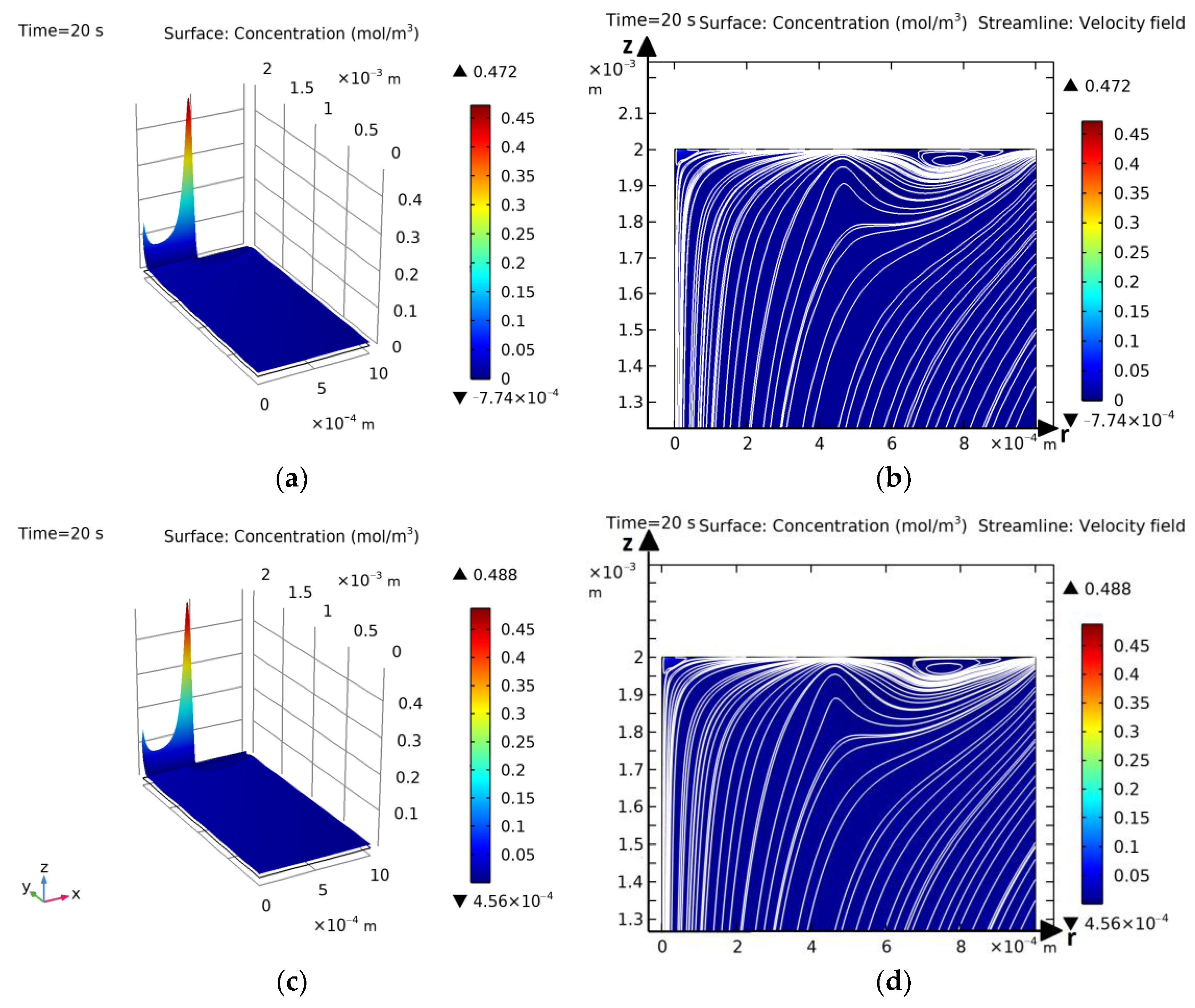
3.1. Computational Experiments for Verification of Hybrid Numerical Method

To verify the results of the proposed hybrid numerical–analytical method, their comparison with the results of an independent numerical solution by the finite element method was used. A large number of computational experiments were carried out with different initial concentrations and angular velocities. An independent numerical solution was performed using the finite element method with a non-uniform grid. When performing the computational experiments, the numbers of elements in the grid varied from 6305 to 147,415 elements. It turned out that a grid consisting of 9581 elements is quite sufficient, since with a larger number of elements, the numerical results do not change, and with a significantly smaller number, they begin to change. A time step of 0.01 s was used.

Comparison of Results for the Annular Disk Model Obtained Using the Hybrid Method and the Independent Finite Element Method

Let us consider the results of the numerical study at the initial concentration $C_0=0.01\mathrm{mol}/{\mathrm{m}}^3$. Figure 2a,b show the graphs of the cation concentration and the solution flow lines for the annular disk model obtained using the hybrid method, and Figure 2c,d show those obtained using the independent finite element method. Figure 3a–d similarly show the results of the numerical study but already at the initial concentration $C_0=0.01 \mathrm{mol}/{\mathrm{m}}^3$. Figure 2a,c and Figure 3a,c show that the maximum concentration occurs near the boundary of the non-conductivity and conductivity regions, and the concentration also increases on the symmetry axis. Figure 2b,d and Figure 3b,d show that vortices are formed in the conductivity region, and the number of vortices increases with increasing concentration.

An animation of the flow (streamlines) near the membrane disk at the initial concentration $C_0=0.01\mathrm{mol}/{\mathrm{m}}^3$ when solved using the hybrid method is given in Supplementary Material Video S1 and when solved using the finite element method in Supplementary Material Video S2.

An animation of the flow (streamlines) near the membrane disk at the initial concentration $C_0=0.01\mathrm{mol}/{\mathrm{m}}^3$ when solved using the hybrid method is given in Supplementary Material Video S3 and when solved using the finite element method in Supplementary Material Video S4.

Thus, at low concentrations in the order of 0.1, 0.01 mol/m³ and less, the finite element method is preferable, and the hybrid method works better with increasing initial concentrations of 0.1, 1, 10 mol/m³ and beyond. In the general area of applicability, the methods lead to results that coincide with an accuracy of about 1%.

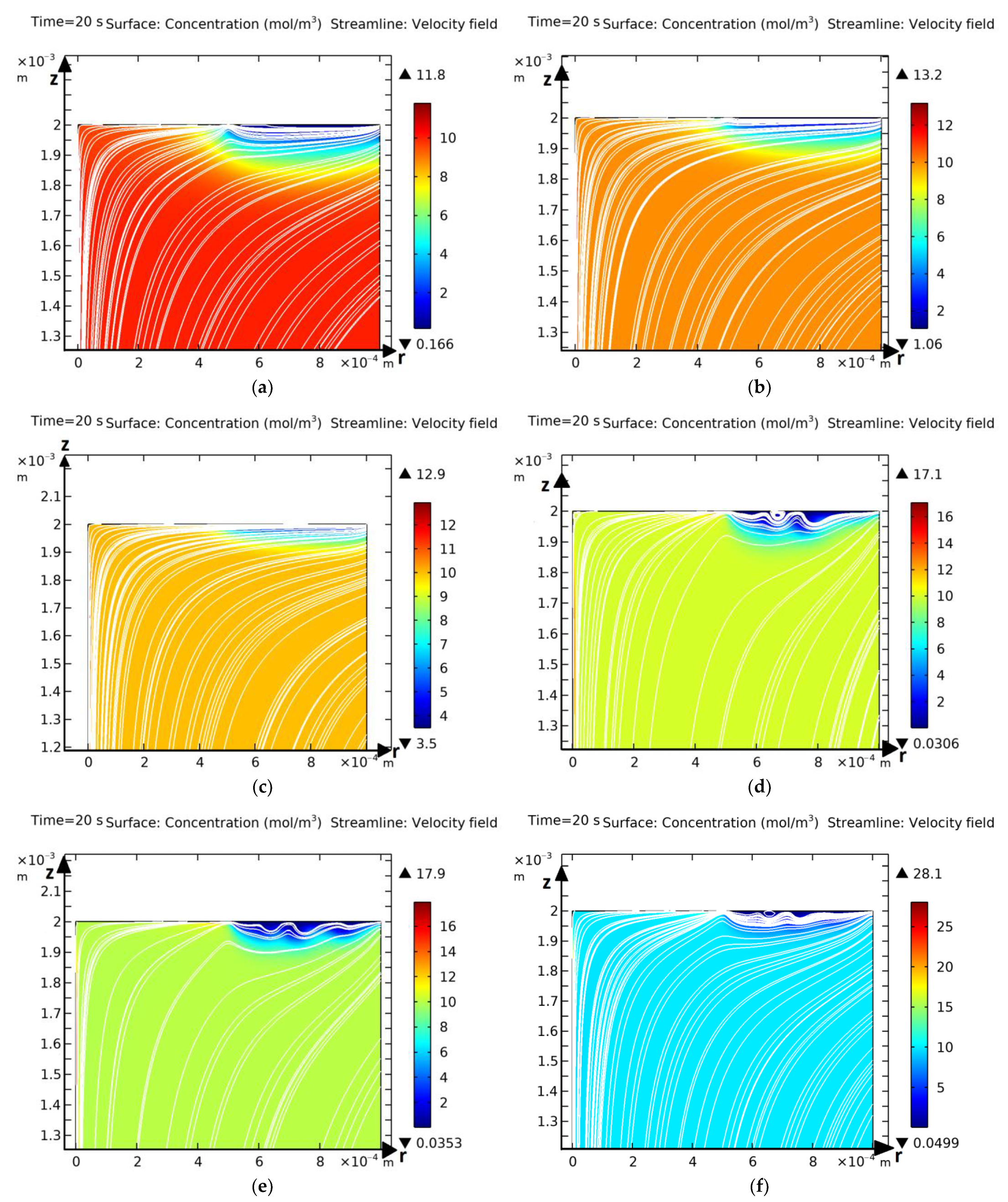
3.2. Basic Laws of Occurrence and Development of Electroconvection and Mass Transfer for the Model with an Annular Membrane

To identify the main patterns, a number of numerical experiments were conducted, with the initial concentrations varying from 0.01 mol/m³ to 100 mol/m³, the angular velocity rates from ${\displaystyle \frac{\pi }{2}}$ to $4\pi$ rad/s, and the potential jump values from 0.1 to 2 V. The most typical results are given below.

Figure 4 shows the solution flow lines at an angular velocity of ${\displaystyle \frac{\pi }{2}}$ rad/s, an initial concentration of 10 mol/m³, and a potential jump of 0.1 V. It is shown that with small potential jumps, vortices do not appear, and the solution flow lines correspond to logarithmic spirals. Additionally, with a small potential jump, a diffusion layer is formed, the thickness of which is approximately constant, with the exception of a small neighborhood near the junction of the non-conductivity and conductivity regions.

Figure 5 shows the results of the study with a potential jump of 0.3 V (Figure 5a–c) and a potential jump of 1.5 V (Figure 5d–f), an initial concentration $C_0=0.01\mathrm{mol}/{\mathrm{m}}^3$, and with variations of the angular velocity of ${\displaystyle \frac{\pi }{2}}$ rad/s (Figure 5a,d), $\pi$ (Figure 5b,e), and $2\pi$ rad/s (Figure 5c,f). It is shown that the greater the angular velocity, the greater the potential jump required for the occurrence of electroconvection.

In real devices, the concentrations are of the order of 10 or more mol/m³, so the results for 1 and 10 mol/m³ are presented below.

Let us consider the case when the initial angular velocity is $\omega ={\displaystyle \frac{\pi }{2}}$ rad/s and the potential jump is $d_{\phi }=1.5$ V. The distribution of the cation concentrations is shown in Figure 6a, where it is evident that the maximum concentration is achieved at the junction of the non-conductivity and conductivity regions. Based on Figure 6b–d, it can be concluded that relaxation associated with the matching of the boundary and initial conditions occurs within 2 s. Vortices arise at the junction of the non-conductivity and conductivity regions and flow downstream, gradually decreasing in size (Figure 6d–e). This is due to the fact that the azimuthal component of the velocity $v=\omega r$ increases with increasing $r$.

An animation of the flow (streamlines) near the membrane disk at the initial concentration $C_0=0.01\mathrm{mol}/{\mathrm{m}}^3$ is shown in Supplementary Material Video S5 and at $C_0=0.01\mathrm{mol}/{\mathrm{m}}^3$ in Supplementary Material Video S6.

4. Discussion

This article proposed a new mathematical model of the influence of inhomogeneity areas on the transfer of salt ions in systems with axial symmetry, taking into account electroconvection in the form of a boundary value problem for a non-stationary coupled system of Nernst–Planck–Poisson and Navier–Stokes equations in a cylindrical coordinate system. An algorithm for a hybrid numerical–analytical solution was formulated, which allows the boundary value problem for real values of the initial concentration, potential jump, and disk rotation speed to be solved. Using the hybrid solution method, the main patterns of occurrence and development of electroconvection and mass transfer for a model with an annular membrane were derived, and the results were verified by comparing them for the annular disk model, obtained using the hybrid method and the independent finite element method.

Using the proposed hybrid method, the process of formation of electroconvective vortices in a potentiostatic mode was numerically studied with the addition of conductivity and non-conductivity regions to a cation exchange rotating membrane disk, including in the form of an annular disk.

It has been established that the vortex formation process can be enhanced by adding non-conductive regions to the CEM, and if the ring membrane model is used, vortices are formed at the junction of non-conductive and conductive regions.

It is shown that with small potential jumps, vortices do not appear, and the solution flow lines correspond to logarithmic spirals. Additionally, with a small potential jump, a diffusion layer is formed, the thickness of which is approximately constant, with the exception of a small neighborhood near the junction of the non-conductivity and conductivity regions. Relaxation associated with the coordination of the boundary and initial conditions occurs within 2 s. Vortices arise at the junction of the non-conductivity and conductivity regions and flow downstream, gradually decreasing in size.

The mathematical models proposed in this article can be used to optimize the desalination process in electromembrane systems with axial symmetry, and the hybrid numerical–analytical method can be applied to solve other boundary problems of membrane electrochemistry.

References

1. Stockmeier, F.; Felder, D.; Eser, S.; Habermann, M.; Peric, P.; Musholt, S.; Albert, K.; Linkhorst, J.; Wessling, M. Localized Electroconvection at Ion-Exchange Membranes with Heterogeneous Surface Charge. Preprint 2021. [Google Scholar] [CrossRef]
2. Bräsel, B.; Yoo, S.-W.; Huber, S.; Wessling, M.; Linkhorst, J. Evolution of particle deposits at communicating membrane pores during crossflow filtration. J. Membr. Sci. 2023, 686, 121977. [Google Scholar] [CrossRef]
3. Seo, M.; Kim, W.; Lee, H.; Kim, S.J. Non-negligible effects of reinforcing structures inside ion exchange membrane on sta-bilization of electroconvective vortices. Desalination 2022, 538, 115902. [Google Scholar] [CrossRef]
4. Ugrozov, V.V.; Filippov, A.N. Resistance of an Ion-Exchange Membrane with a Surface-Modified Charged Layer. Colloid J. 2022, 84, 761–768. [Google Scholar] [CrossRef]
5. Kovalenko, A.V.; Yzdenova, A.M.; Sukhinov, A.I.; Chubyr, N.O.; Urtenov, M.K. Simulation of galvanic dynamic mode in membrane hydrocleaning systems taking into account space charge. AIP Conf. Proc. 2019, 2188, 050021. [Google Scholar] [CrossRef]
6. Urtenov, M.K.; Kovalenko, A.V.; Sukhinov, A.I.; Chubyr, N.O.; Gudza, V.A. Model and numerical experiment for calculating the theoretical current-voltage characteristic in electro-membrane systems. Iop Conf. Ser. Mater. Sci. Eng. 2019, 680, 012030. [Google Scholar] [CrossRef]
7. Filippov, A.N.; Akberova, E.M.; Vasil’eva, V.I. Study of the Thermochemical Effect on the Transport and Structural Charac-teristics of Heterogeneous Ion-Exchange Membranes by Combining the Cell Model and the Fine-Porous Membrane Model. Polymers 2023, 15, 3390. [Google Scholar] [CrossRef] [PubMed]
8. Mai, Z.; Fan, S.; Wang, Y.; Chen, J.; Chen, Y.; Bai, K.; Deng, L.; Xiao, Z. Catalytic nanofiber composite membrane by combining electrospinning precursor seeding and flowing synthesis for immobilizing ZIF-8 derived Ag nanoparticles. J. Membr. Sci. 2022, 643, 120045. [Google Scholar] [CrossRef]
9. Stockmeier, F.; Stüwe, L.; Kneppeck, C.; Musholt, S.; Albert, K.; Linkhorst, J.; Wessling, M. On the interaction of electroconvection at a membrane interface with the bulk flow in a spacer-filled feed channel. J. Membr. Sci. 2023, 678, 121589. [Google Scholar] [CrossRef]
10. Zaltzman, B.; Rubinstein, I. Electro-osmotic slip and electroconvection at heterogeneous ion-exchange membranes. J. Fluid Mech. 2007, 579, 173–226. [Google Scholar] [CrossRef]
11. Rubinstein, I.; Zaltzman, B. How the fine structure of the electric double layer and the flow affect morphological instability in electrodeposition. Phys. Rev. Fluids 2023, 8, 093701. [Google Scholar] [CrossRef]
12. Choi, J.; Cho, M.; Shin, J.; Kwak, R.; Kim, B. Electroconvective instability at the surface of one-dimensionally patterned ion exchange membranes. J. Membr. Sci. 2024, 691, 122256. [Google Scholar] [CrossRef]
13. Gupta, A.; Zuk, P.J.; Stone, H.A. Charging Dynamics of Overlapping Double Layers in a Cylindrical Nanopore. Phys. Rev. Lett. 2020, 125, 076001. [Google Scholar] [CrossRef] [PubMed]
14. Kozmai, A.; Mareev, S.A.; Butylskii, D.; Ruleva, V.; Pismenskaya, N.; Nikonenko, V. Low-frequency impedance of ion-exchange membrane with electrically heterogeneous surface. Electrochim. Acta 2023, 451, 142285. [Google Scholar] [CrossRef]
15. Vasilieva, V.I.; Meshcheryakova, E.E.; Falina, I.V.; Kononenko, N.A.; Brovkina, M.A.; Akberova, E.M. Effect of Heterogeneous Ion-Exchange Membranes Composition on Their Structure and Transport Properties. Membr. Membr. Technol. 2023, 5, 139–147. [Google Scholar] [CrossRef]
16. Kazakovtseva, E.V.; Kovalenko, A.V.; Pismenskiy, A.V.; Urtenov, M.A.H. Hybrid numerical-analytical method for solving the problems of salt ion transport in membrane systems with axial symmetry. J. Samara State Tech. Univ. Ser. Phys. Math. Sci. 2024, 28, 130–151. [Google Scholar] [CrossRef]
17. Grafov, B.M.; Chernenko, A.A. Passage of direct current through a binary electrolyte solution. J. Phys. Chem. 1963, 37, 664. [Google Scholar]
18. Newman, J. Electrochemical Systems. World 1977. 463p. Available online: https://books.google.com.hk/books/about/Electrochemical_Systems.html?id=vArZu0HM-xYC&redir_esc=y (accessed on 10 June 2025).
19. Doolan, E.; Miller, J.; Shields, W. Uniform Numerical Methods for Solving Boundary Layer Problems; Mir: Moscow, Russia, 1983; p. 199. [Google Scholar]
Figure 1. The studied area, its cross-section, and its boundaries: (a) general view; (b) half of the cross-section, where 1 is the axis of symmetry, 2 is the depth of the solution, 3 and 4 represent the cation exchange membrane, and 5 is the open boundary. The conductive region of the membrane is shown in gray.
Inventions 10 00050 g001
Figure 2. Graphs at initial concentration C 0 = 0.01 mol / m 3 : (a) cation concentration when solved using the hybrid method; (b) solution flow lines near the membrane when solved using the hybrid method; (c) cation concentration when solved using the independent finite element method; (d) solution flow lines near the membrane using the independent finite element method.
Inventions 10 00050 g002
Figure 3. Graphs at initial concentration C 0 = 0.01 mol / m 3 : (a) cation concentration when solved using the hybrid method; (b) solution flow lines near the membrane when solved using the hybrid method; (c) cation concentration when solved using the independent finite element method; (d) solution flow lines near the membrane using the independent finite element method.
Inventions 10 00050 g003
Figure 4. Solution current lines at a potential jump of 0.1 V: (a) general view; (b) near the membrane.
Inventions 10 00050 g004
Figure 5. Graph of solution flow lines near the membrane disk: (a) at d φ = 0.3 V and angular velocity π 2 rad/s; (b) at d φ = 0.3 V and angular velocity π rad/s; (c) at d φ = 0.3 V and angular velocity 2 π rad/s; (d) at d φ = 1.5 V and angular velocity π 2 rad/s; (e) at d φ = 1.5 V and angular velocity π rad/s; (f) at d φ = 1.5 V and angular velocity 2 π rad/s.
Inventions 10 00050 g005
Figure 6. Graphs of the (a) cation concentration at C 0 = 0.01 mol / m 3 , (b) solution flow lines near the membrane at C 0 = 0.01 mol / m 3 and t = 1 s, (c) solution flow lines near the membrane at C 0 = 0.01 mol / m 3 and t = 2 s, (d) solution flow lines near the membrane at C 0 = 0.01 mol / m 3 and t = 20 s, and (e) solution flow lines near the membrane at C 0 = 0.01 mol / m 3 and t = 20 s.
Inventions 10 00050 g006